The Mass and the Tuning of the Composite Higgs · The Mass and the Tuning of the Composite Higgs....
38
Andrea Wulzer Galileo Galilei DIPARTIMENTO DI FISICA E ASTRONOMIA D A F The Mass and the Tuning of the Composite Higgs
Transcript of The Mass and the Tuning of the Composite Higgs · The Mass and the Tuning of the Composite Higgs....
Andrea Wulzer
Galileo Galilei
DIPARTIMENTO DI FISICAE ASTRONOMIA
DAF
The Mass and the Tuning of the Composite Higgs
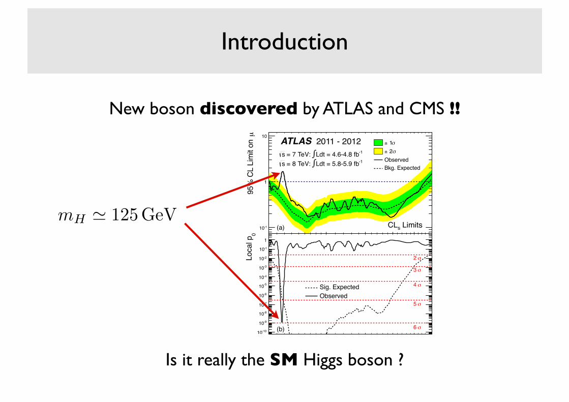
New boson discovered by ATLAS and CMS !!
200 300 400 500
µ95
% C
L Li
mit
on
-110
1
10σ 1±
σ 2±
ObservedBkg. Expected
ATLAS 2011 - 2012-1Ldt = 4.6-4.8 fb∫ = 7 TeV: s -1Ldt = 5.8-5.9 fb∫ = 8 TeV: s
LimitssCL(a)
0Lo
cal p
-1010
-910
-810
-710
-610
-510
-410
-310
-210
-110
1
Sig. ExpectedObserved
(b)
σ2
σ3
σ4
σ5
σ6
[GeV]Hm200 300 400 500
)µ
Sign
al s
treng
th (
-1
-0.5
0
0.5
1
1.5
2
Observed)<1µ(λ-2 ln (c)
110 150
Figure 7: Combined search results: (a) The observed (solid) 95% CLlimits on the signal strength as a function of mH and the expec-tation (dashed) under the background-only hypothesis. The darkand light shaded bands show the ±1! and ±2! uncertainties on thebackground-only expectation. (b) The observed (solid) local p0 as afunction of mH and the expectation (dashed) for a SM Higgs bosonsignal hypothesis (µ = 1) at the given mass. (c) The best-fit signalstrength µ̂ as a function of mH . The band indicates the approximate68% CL interval around the fitted value.
provide fully reconstructed candidates with high reso-lution in invariant mass, as shown in Figures 8(a) and8(b). These excesses are confirmed by the highly sen-sitive but low-resolution H!WW (")! "#"# channel, asshown in Fig. 8(c).The observed local p0 values from the combination
of channels, using the asymptotic approximation, areshown as a function of mH in Fig. 7(b) for the full massrange and in Fig. 9 for the low mass range.The largest local significance for the combination of
the 7 and 8 TeV data is found for a SM Higgs bosonmass hypothesis of mH=126.5GeV, where it reaches6.0!, with an expected value in the presence of a SMHiggs boson signal at that mass of 4.9! (see also Ta-ble 7). For the 2012 data alone, the maximum lo-cal significance for the H!ZZ(")! 4", H! $$ and
110 115 120 125 130 135 140 145 150
0Lo
cal p
-710
-610
-510
-410
-310
-210
-110
1
10 ATLAS 2011 - 2012 4l→ (*) ZZ→(a) H
σ2
σ3
σ4
σ5
-1Ldt = 4.8 fb∫ = 7 TeV: s -1Ldt = 5.8 fb∫ = 8 TeV: s
110 115 120 125 130 135 140 145 150
0Lo
cal p
-710
-610
-510
-410
-310
-210
-110
1
10γγ →(b) H
σ2
σ3
σ4
σ5
-1Ldt = 4.8 fb∫ = 7 TeV: s -1Ldt = 5.9 fb∫ = 8 TeV: s
[GeV]Hm110 115 120 125 130 135 140 145
0Lo
cal p
-910
-810
-710
-610
-510
-410
-310
-210
-1101
10νlν l→ (*) WW→(c) H
σ2
σ3 σ4
σ5
2011 Exp.2011 Obs.
2012 Exp.2012 Obs.
2011-2012 Exp.2011-2012 Obs.
-1Ldt = 4.7 fb∫ = 7 TeV: s -1Ldt = 5.8 fb∫ = 8 TeV: s
Figure 8: The observed local p0 as a function of the hypothesizedHiggs boson mass for the (a) H!ZZ(")! 4", (b) H! $$ and (c)H!WW(")! "#"# channels. The dashed curves show the expectedlocal p0 under the hypothesis of a SMHiggs boson signal at that mass.Results are shown separately for the
#s = 7TeV data (dark, blue), the#
s = 8TeV data (light, red), and their combination (black).
H!WW (")! e#µ# channels combined is 4.9!, and oc-curs at mH = 126.5GeV (3.8! expected).
The significance of the excess is mildly sensitive touncertainties in the energy resolutions and energy scalesystematic uncertainties for photons and electrons; thee!ect of the muon energy scale systematic uncertain-ties is negligible. The presence of these uncertainties,evaluated as described in Ref. [138], reduces the localsignificance to 5.9!.
The global significance of a local 5.9! excess any-where in the mass range 110–600GeV is estimated tobe approximately 5.1!, increasing to 5.3! in the range110–150GeV, which is approximately the mass rangenot excluded at the 99% CL by the LHC combined SMHiggs boson search [139] and the indirect constraintsfrom the global fit to precision electroweak measure-ments [12].
18
Introduction
mH ' 125GeV
Is it really the SM Higgs boson ?
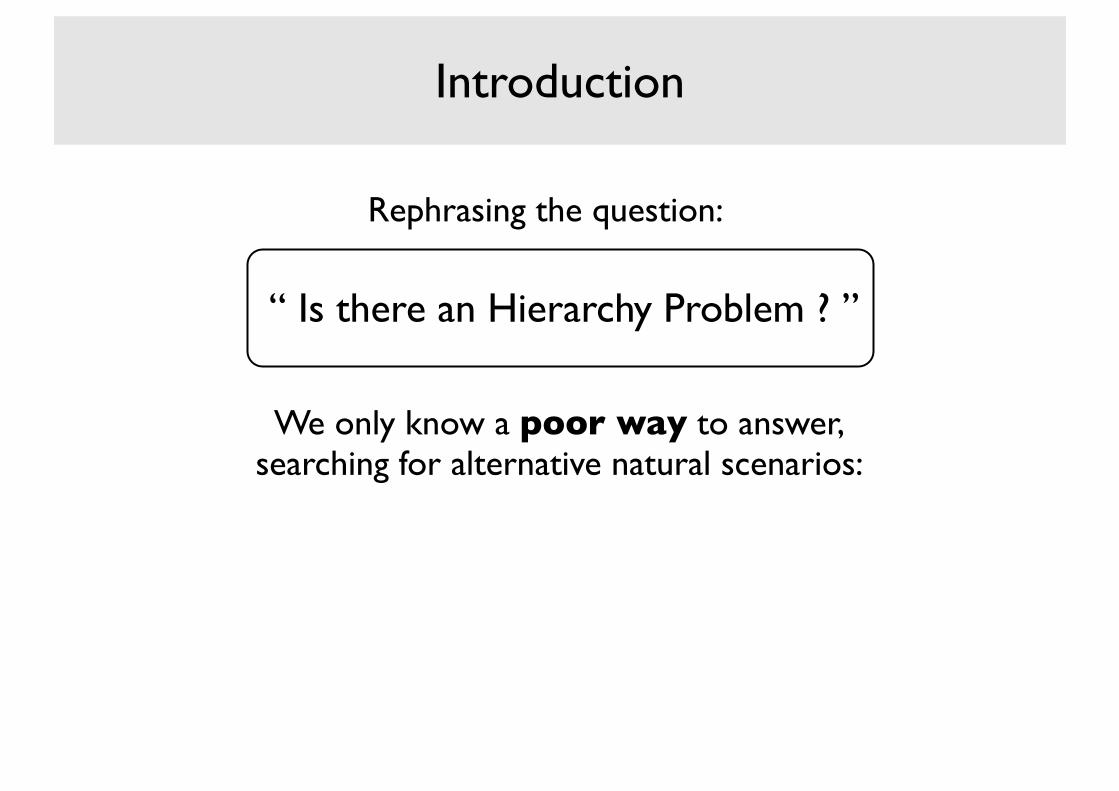
“ Is there an Hierarchy Problem ? ”
Rephrasing the question:
Introduction
We only know a poor way to answer,searching for alternative natural scenarios:
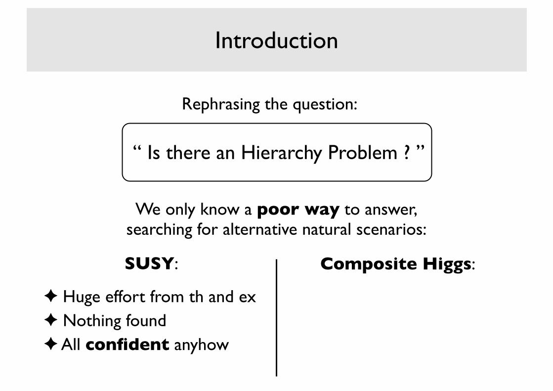
“ Is there an Hierarchy Problem ? ”
Introduction
We only know a poor way to answer,searching for alternative natural scenarios:
SUSY:
✦ Huge effort from th and ex✦ Nothing found✦ All confident anyhow
Composite Higgs:
Rephrasing the question:
“ Is there an Hierarchy Problem ? ”
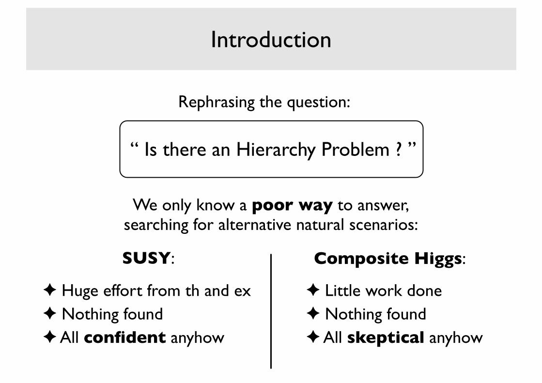
Introduction
We only know a poor way to answer,searching for alternative natural scenarios:
SUSY:
✦ Huge effort from th and ex✦ Nothing found✦ All confident anyhow
✦ Little work done✦ Nothing found✦ All skeptical anyhow
Composite Higgs:
Rephrasing the question:
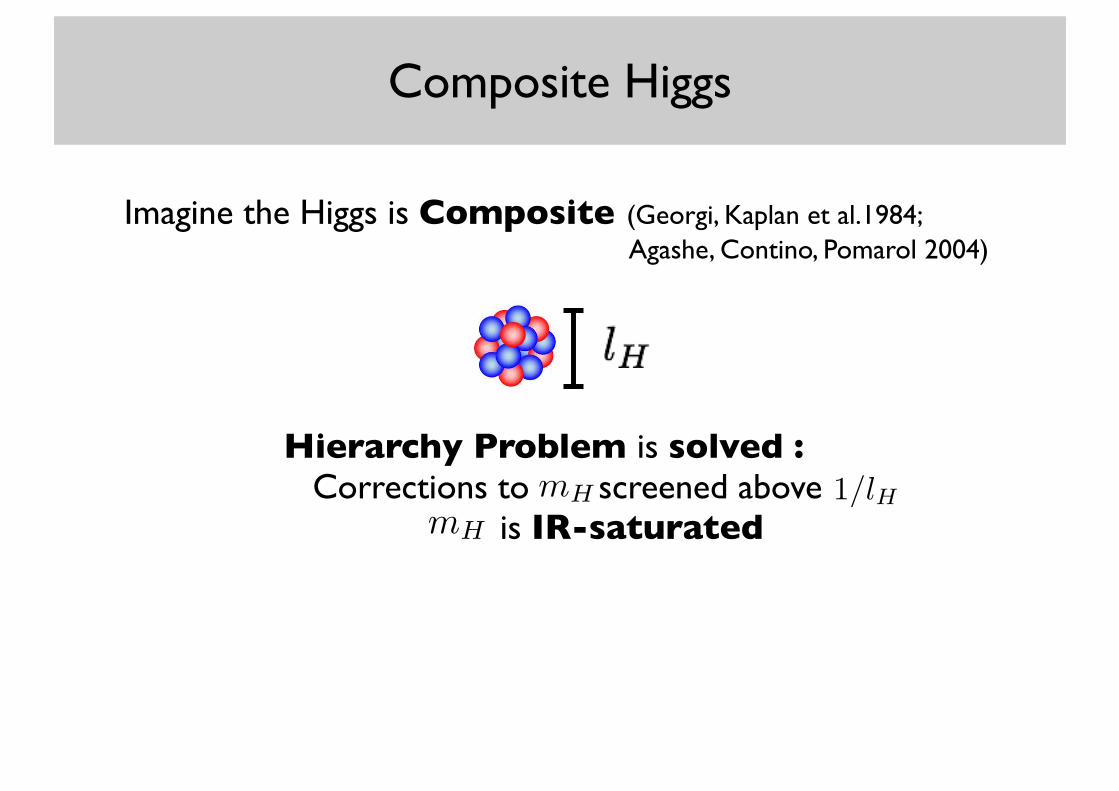
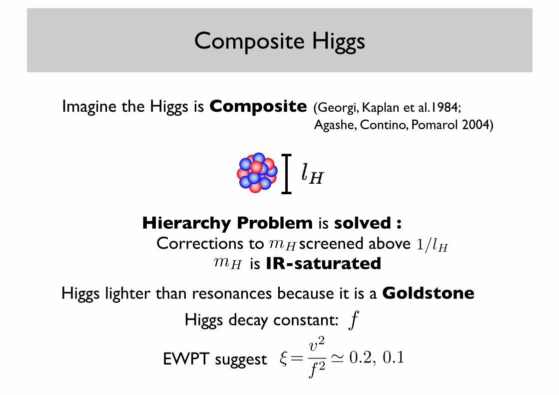
Composite Higgs
Imagine the Higgs is Composite (Georgi, Kaplan et al.1984; Agashe, Contino, Pomarol 2004)
Hierarchy Problem is solved :Corrections to screened above \
is IR-saturated1/lHmH
mH
Composite Higgs
Imagine the Higgs is Composite (Georgi, Kaplan et al.1984; Agashe, Contino, Pomarol 2004)
Hierarchy Problem is solved :Corrections to screened above \
is IR-saturated1/lHmH
mH
Higgs lighter than resonances because it is a Goldstone
Higgs decay constant: f
EWPT suggest ⇠=v2
f2' 0.2, 0.1
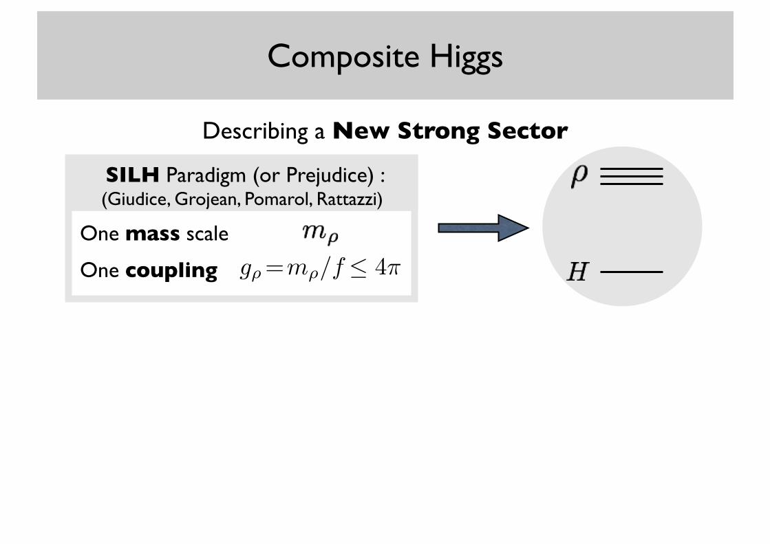
Composite Higgs
Describing a New Strong Sector
SILH Paradigm (or Prejudice) :(Giudice, Grojean, Pomarol, Rattazzi)
One mass scale
One coupling g⇢=m⇢/f 4⇡
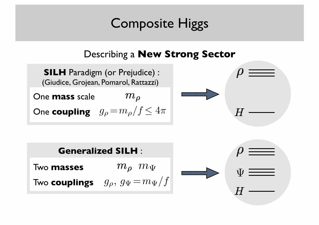
Composite Higgs
Describing a New Strong Sector
g⇢=m⇢/f 4⇡
Generalized SILH :
Two masses
Two couplings
m g⇢, g =m /f
SILH Paradigm (or Prejudice) :(Giudice, Grojean, Pomarol, Rattazzi)
One mass scale
One coupling
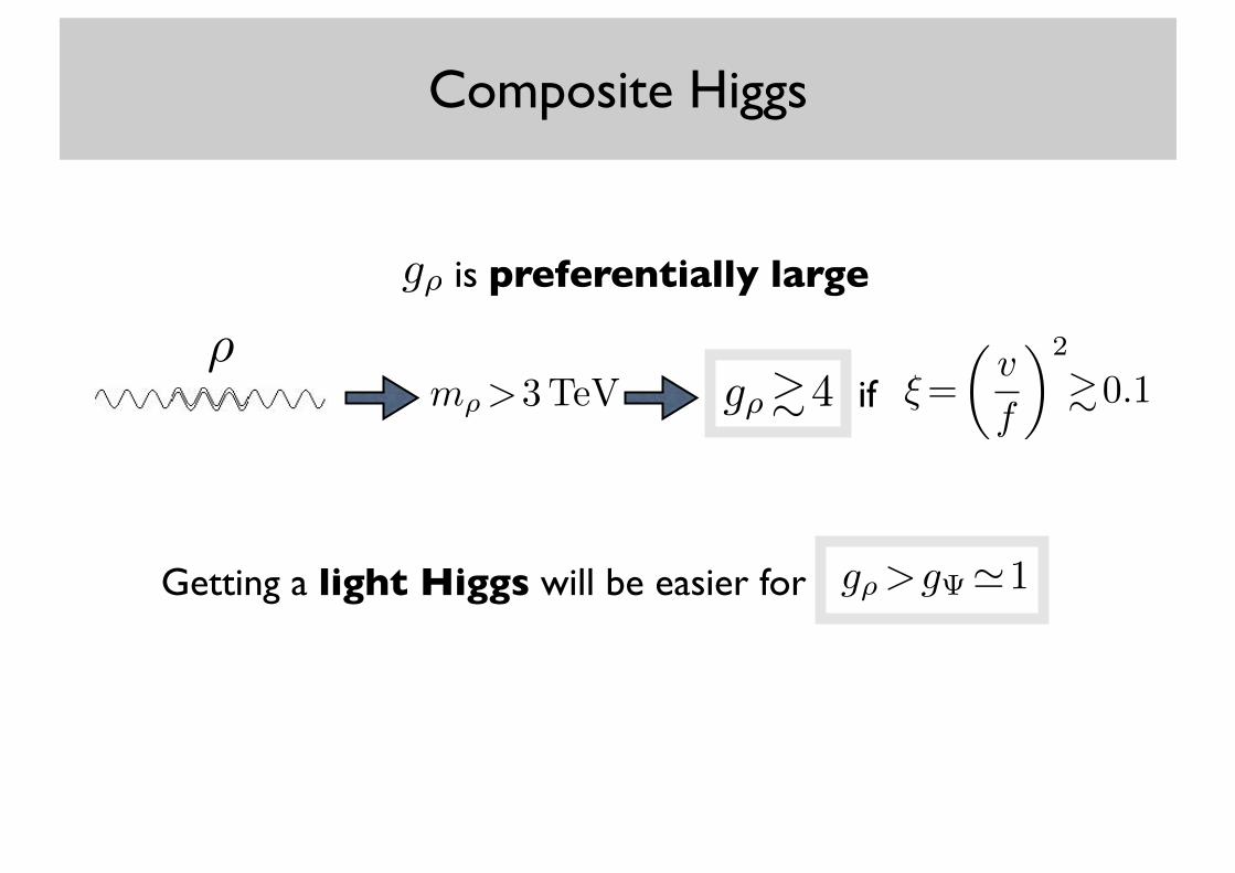
Composite Higgs
⇢
is preferentially largeg⇢
g⇢&4 if ⇠=
✓v
f
◆2
&0.1
Getting a light Higgs will be easier for
m⇢>3TeV
g⇢>g '1
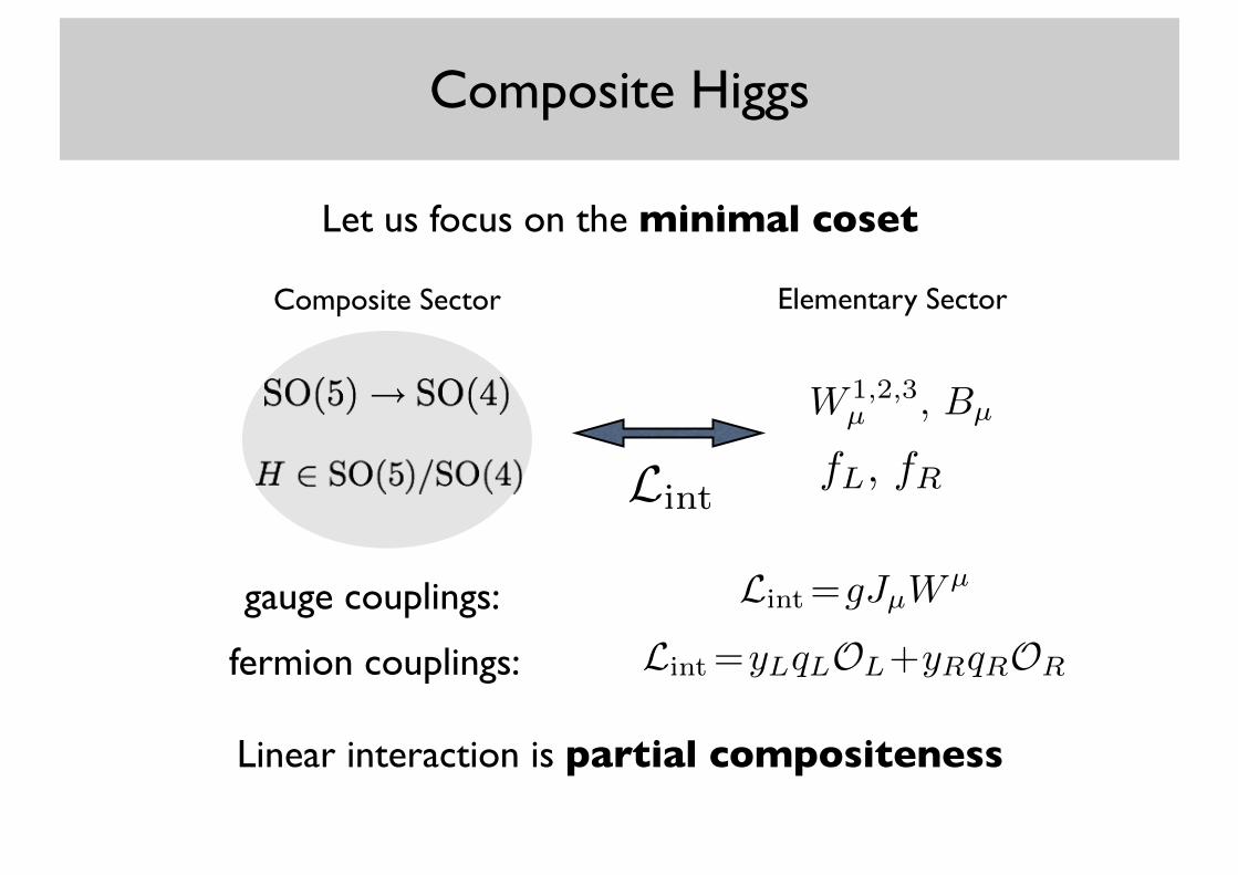
Let us focus on the minimal coset
Composite Sector Elementary Sector
fL, fR
W 1,2,3µ , Bµ
Lint
gauge couplings:
fermion couplings:
Lint=gJµWµ
Lint=yLqLOL+yRqROR
Composite Higgs
Linear interaction is partial compositeness
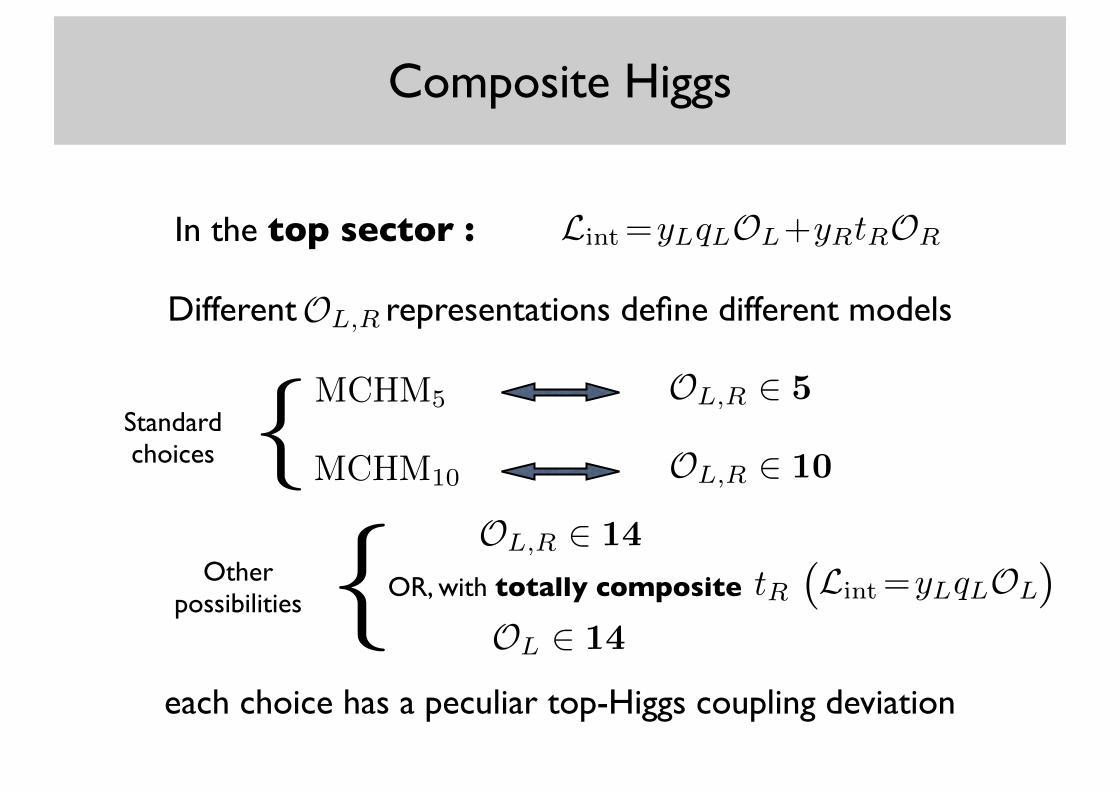
Composite Higgs
MCHM5
MCHM10
OL,R 2 5
OL,R 2 10
OL,RDifferent representations define different models
{Standard choices
{Otherpossibilities
OL,R 2 14
OR, with totally composite tR
OL 2 14
Lint=yLqLOL+yRtRORIn the top sector :
each choice has a peculiar top-Higgs coupling deviation
Lint=yLqLOL+yRtROR( )
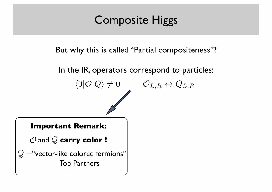
Composite Higgs
OL,R $ QL,Rh0|O|Qi 6= 0
Important Remark:
and carry color !O Q
Q =“vector-like colored fermions”
In the IR, operators correspond to particles:
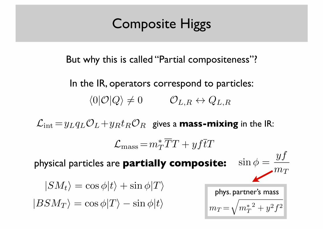
But why this is called “Partial compositeness”?
Top Partners
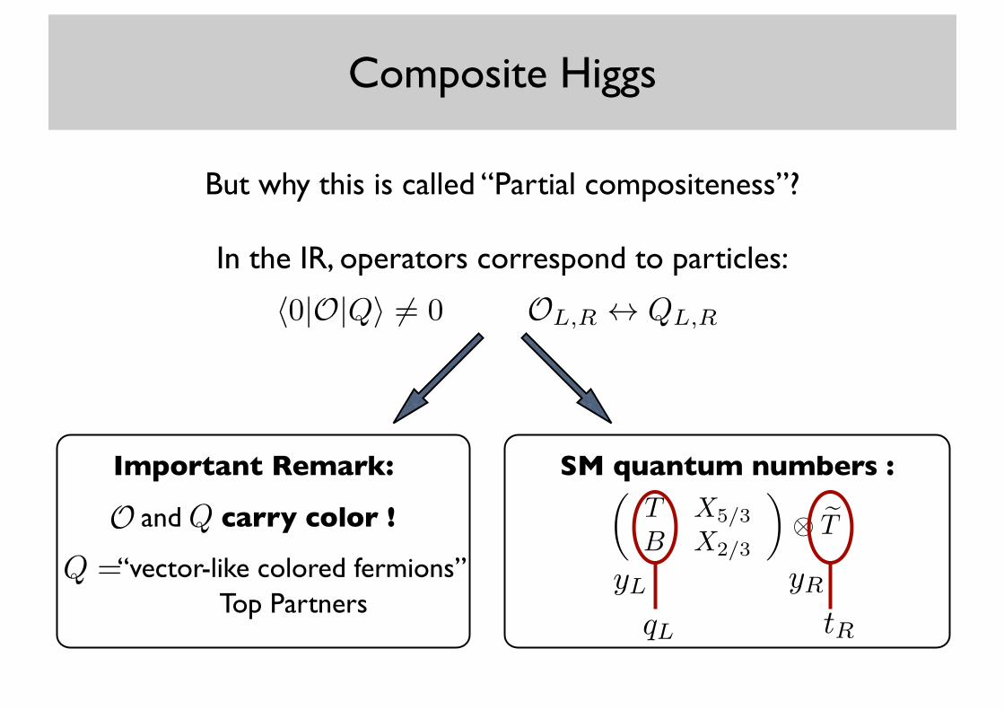
Composite Higgs
, e 2 5 =
✓T X5/3
B X2/3
◆⌦ eT
OL,R $ QL,Rh0|O|Qi 6= 0
Important Remark:
and carry color !O Q
Q =“vector-like colored fermions”
In the IR, operators correspond to particles:
But why this is called “Partial compositeness”?
Top Partners
SM quantum numbers :
qL
yLtR
yR
Composite Higgs
OL,R $ QL,Rh0|O|Qi 6= 0
In the IR, operators correspond to particles:
But why this is called “Partial compositeness”?
Lint=yLqLOL+yRtROR gives a mass-mixing in the IR:
physical particles are partially composite:
|SMti = cos�|ti+ sin�|T i
|BSMT i = cos�|T i � sin�|ti
Lmass=m⇤TTT + yftT
sin� =yf
mT
phys. partner’s mass
mT =qm⇤
T2 + y2f2
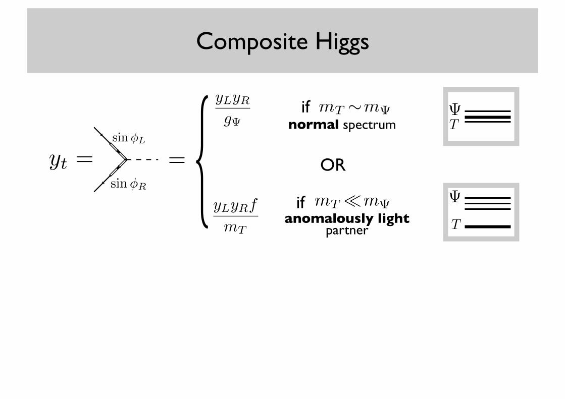
Composite Higgs
yt = = {yLyRg
yLyRf
mT
mT ⇠m
mT ⌧m
if
if
normal spectrum
anomalously light partner
OR
T
T
sin�L
sin�R
Composite Higgs
yt = = {yLyRg
yLyRf
mT
mT ⇠m
mT ⌧m
if
if
normal spectrum
anomalously light partner
For yL ' yR
OR
{ OR
y=pytg be careful with saturation
mT =qm⇤
T2 + y2f2 �yf
y �yty=
rytmT
f
T
T
sin�L
sin�R
Mass and Tuning
........
yR are the Left- and Right-handed fermion linear couplings, which we will denote as “proto-Yukawa”
couplings. Schematically, the couplings of the elementary fields to the strong sector can be written as
Lmix = gSM · ⇥SM · O , (1)
where ⇥SM = (Aµ, f) collectively denotes the SM gauge fields and fermions. Notice that, since the ele-
mentary state do not fill complete representation of G, Lmix unavoidably breaks the strong sector’s global
group. The Higgs therefore becomes a Pseudo-NGB (PNGB) and is free to acquire a potential, as we will
discuss in sect. 2.4.
Because of these linear couplings, the SM fields acquire a composite component which is proportional
to the degree of mixing ⌃g = g/g� and ⌃L,R = yL,R/g� with the strong sector’s resonances. It is only when
this composite component is not too large that the previously-mentioned phenomenological bounds can
be accommodated and the model made realistic. This suggests that the coupling g� is better taken to be
large, at least larger than the SM couplings gSM . As in [2], we then restrict our parameter space to the
region
gSM ⇤ g� ⇤ 4⇥ ,
where the limit of total compositeness gSM = g� can only be considered for the tR (yR = g�), given that
phenomenological constraint on the tR compositeness are practically absent. Instead of taking yR = g�,
a more direct way to achieve total tR compositeness is not to introduce the elementary tR field to start
with, and assume that a massless resonance with the quantum numbers of the tR emerges from the strong
sector.
2.2 An issue with T̂{Tissue}
In the Standard Model with an elementary Higgs boson, the accidental SO(4) symmetry of the Higgs
sector ensures the survival, after electro-weak symmetry breaking, of an (approximate) custodial isospin
SO(3)c. This symmetry is essential to successfully reproduce electro-weak precision data, in particular the
relation ⇤ ⇥ m2W /m2
Z cos2 �W ⌅ 1, or equivalently the bound on T̂ , see [2] for the conventions. In the
minimal composite Higgs model based on SO(5)/SO(4) the SO(4) symmetry is a true symmetry of strong
dynamics, satisfied by all the non-linear ⌅ model interactions. Then, the Higgs field being a 4 of SO(4),
the generic vacuum will again respect a residual custodial SO(3)c. On the other hand, in non-minimal
models with two Higgses in the 4 of SO(4) the generic residual symmetry will only be SO(2)c. This is
because the scalar potential, generated by SO(4) breaking interactions (for instance the top Yukawa or
the SM gauge couplings) will in general only respects the SU(2)L � U(1)Y subgroup of SO(4). 6 Thus
even though the nonlinear interactions satisfy SO(4), an unacceptable contribution to T̂ will arise for a
generic vacuum structure. To discuss this problem in more detail, it is useful to use two parametrizations
of a 4 of SO(4), the one as a 4-vector � = {⇧i}, i = 1, . . . , 4 and the one as a 2� 2 matrix � ⇥ ⇧4 + i⇧k⌅k
6The unbroken SO(2)c should of course coincide with U(1)Q in order to avoid a worse phenomenological problem.
7
. . .
yR are the Left- and Right-handed fermion linear couplings, which we will denote as “proto-Yukawa”
couplings. Schematically, the couplings of the elementary fields to the strong sector can be written as
Lmix = gSM · ⇥SM · O , (1)
where ⇥SM = (Aµ, f) collectively denotes the SM gauge fields and fermions. Notice that, since the ele-
mentary state do not fill complete representation of G, Lmix unavoidably breaks the strong sector’s global
group. The Higgs therefore becomes a Pseudo-NGB (PNGB) and is free to acquire a potential, as we will
discuss in sect. 2.4.
Because of these linear couplings, the SM fields acquire a composite component which is proportional
to the degree of mixing ⌃g = g/g� and ⌃L,R = yL,R/g� with the strong sector’s resonances. It is only when
this composite component is not too large that the previously-mentioned phenomenological bounds can
be accommodated and the model made realistic. This suggests that the coupling g� is better taken to be
large, at least larger than the SM couplings gSM . As in [2], we then restrict our parameter space to the
region
gSM ⇤ g� ⇤ 4⇥ ,
where the limit of total compositeness gSM = g� can only be considered for the tR (yR = g�), given that
phenomenological constraint on the tR compositeness are practically absent. Instead of taking yR = g�,
a more direct way to achieve total tR compositeness is not to introduce the elementary tR field to start
with, and assume that a massless resonance with the quantum numbers of the tR emerges from the strong
sector.
2.2 An issue with T̂{Tissue}
In the Standard Model with an elementary Higgs boson, the accidental SO(4) symmetry of the Higgs
sector ensures the survival, after electro-weak symmetry breaking, of an (approximate) custodial isospin
SO(3)c. This symmetry is essential to successfully reproduce electro-weak precision data, in particular the
relation ⇤ ⇥ m2W /m2
Z cos2 �W ⌅ 1, or equivalently the bound on T̂ , see [2] for the conventions. In the
minimal composite Higgs model based on SO(5)/SO(4) the SO(4) symmetry is a true symmetry of strong
dynamics, satisfied by all the non-linear ⌅ model interactions. Then, the Higgs field being a 4 of SO(4),
the generic vacuum will again respect a residual custodial SO(3)c. On the other hand, in non-minimal
models with two Higgses in the 4 of SO(4) the generic residual symmetry will only be SO(2)c. This is
because the scalar potential, generated by SO(4) breaking interactions (for instance the top Yukawa or
the SM gauge couplings) will in general only respects the SU(2)L � U(1)Y subgroup of SO(4). 6 Thus
even though the nonlinear interactions satisfy SO(4), an unacceptable contribution to T̂ will arise for a
generic vacuum structure. To discuss this problem in more detail, it is useful to use two parametrizations
of a 4 of SO(4), the one as a 4-vector � = {⇧i}, i = 1, . . . , 4 and the one as a 2� 2 matrix � ⇥ ⇧4 + i⇧k⌅k
6The unbroken SO(2)c should of course coincide with U(1)Q in order to avoid a worse phenomenological problem.
7
+ . . .
yR are the Left- and Right-handed fermion linear couplings, which we will denote as “proto-Yukawa”
couplings. Schematically, the couplings of the elementary fields to the strong sector can be written as
Lmix = gSM · ⇥SM · O , (1)
where ⇥SM = (Aµ, f) collectively denotes the SM gauge fields and fermions. Notice that, since the ele-
mentary state do not fill complete representation of G, Lmix unavoidably breaks the strong sector’s global
group. The Higgs therefore becomes a Pseudo-NGB (PNGB) and is free to acquire a potential, as we will
discuss in sect. 2.4.
Because of these linear couplings, the SM fields acquire a composite component which is proportional
to the degree of mixing ⌃g = g/g� and ⌃L,R = yL,R/g� with the strong sector’s resonances. It is only when
this composite component is not too large that the previously-mentioned phenomenological bounds can
be accommodated and the model made realistic. This suggests that the coupling g� is better taken to be
large, at least larger than the SM couplings gSM . As in [2], we then restrict our parameter space to the
region
gSM ⇤ g� ⇤ 4⇥ ,
where the limit of total compositeness gSM = g� can only be considered for the tR (yR = g�), given that
phenomenological constraint on the tR compositeness are practically absent. Instead of taking yR = g�,
a more direct way to achieve total tR compositeness is not to introduce the elementary tR field to start
with, and assume that a massless resonance with the quantum numbers of the tR emerges from the strong
sector.
2.2 An issue with T̂{Tissue}
In the Standard Model with an elementary Higgs boson, the accidental SO(4) symmetry of the Higgs
sector ensures the survival, after electro-weak symmetry breaking, of an (approximate) custodial isospin
SO(3)c. This symmetry is essential to successfully reproduce electro-weak precision data, in particular the
relation ⇤ ⇥ m2W /m2
Z cos2 �W ⌅ 1, or equivalently the bound on T̂ , see [2] for the conventions. In the
minimal composite Higgs model based on SO(5)/SO(4) the SO(4) symmetry is a true symmetry of strong
dynamics, satisfied by all the non-linear ⌅ model interactions. Then, the Higgs field being a 4 of SO(4),
the generic vacuum will again respect a residual custodial SO(3)c. On the other hand, in non-minimal
models with two Higgses in the 4 of SO(4) the generic residual symmetry will only be SO(2)c. This is
because the scalar potential, generated by SO(4) breaking interactions (for instance the top Yukawa or
the SM gauge couplings) will in general only respects the SU(2)L � U(1)Y subgroup of SO(4). 6 Thus
even though the nonlinear interactions satisfy SO(4), an unacceptable contribution to T̂ will arise for a
generic vacuum structure. To discuss this problem in more detail, it is useful to use two parametrizations
of a 4 of SO(4), the one as a 4-vector � = {⇧i}, i = 1, . . . , 4 and the one as a 2� 2 matrix � ⇥ ⇧4 + i⇧k⌅k
6The unbroken SO(2)c should of course coincide with U(1)Q in order to avoid a worse phenomenological problem.
7
+
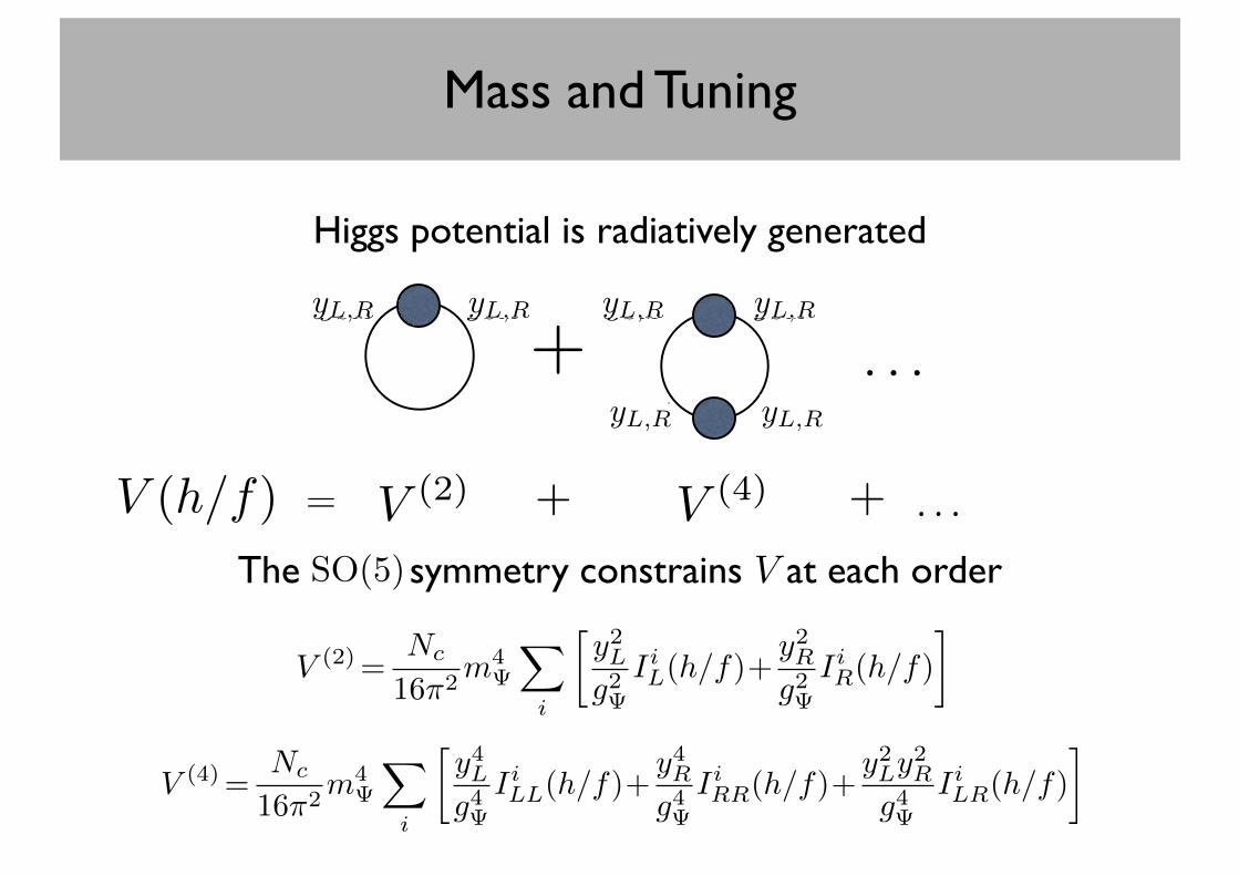
Figure 2: Power counting for the Higgs potential.
Due to the couplings in eq. (2) to the SM fermions, and in particular to the quarks, the strong sector
must be charged under the full SM group, including the color SU(3)c. On top of the G/H cosets discussed
until now, and listed in table 1, the strong sector must therefore also enjoy an unbroken SU(3)c global
group, weakly gauged with coupling gstrong
by elementary gluon fields. This gluon gauge coupling should
also appear in eq. (2), but it will be ignored since it does not play any role in what follows. Another
unbroken symmetry of the strong sector that we have not mentioned is the strong sector matter charge
U(1)X , which is needed to assign the correct hypercharge to the fermionic operators. The hypercharge is
identified as Y = T 3
R +X, in terms of the third SU(2)R generator T 3
R.
The Structure of the Potential
Let us briefly recall, for future use, the general structure of the e↵ective potential of our PNGB Higgs.
In general, given a strong sector, one could imagine breaking its global symmetry G either by adding
new weak interactions among the composites or by their direct (weak) coupling to external elementary
fields. For instance, in QCD the chiral symmetry is broken both by fermion masses, belonging to the first
class of couplings, and by the coupling of quarks to the photon, which belongs to the second class. In our
composite Higgs scenario, as described above, the second class of e↵ects is always unavoidably present,
while the first is not. It is thus not unreasonable, and also motivated by simplicity, to assume all the
breaking of G is due to the coupling to the SM fields in eq. (2). We will work under this assumption,
bearing however in mind that by relaxing the latter the parameter space of PNGB Higgs models could be
significantly enlarged.
Thanks to the above assumption, the potential only originates from insertions of the gSM couplings of
eq. (2), and much can be said on its structure. First of all, its size can be estimated, as figure 2 shows, in
an expansion in loops and in powers of the degree of the mixing ✏ = gSM/g⇢. By noticing that each strong
sector’s hO . . .Oi correlator (represented as a circle in figure 2) is proportional to 1/g2⇢ / N , the estimate
7
yL,R
yL,R yL,R
yL,RyL,RyL,R
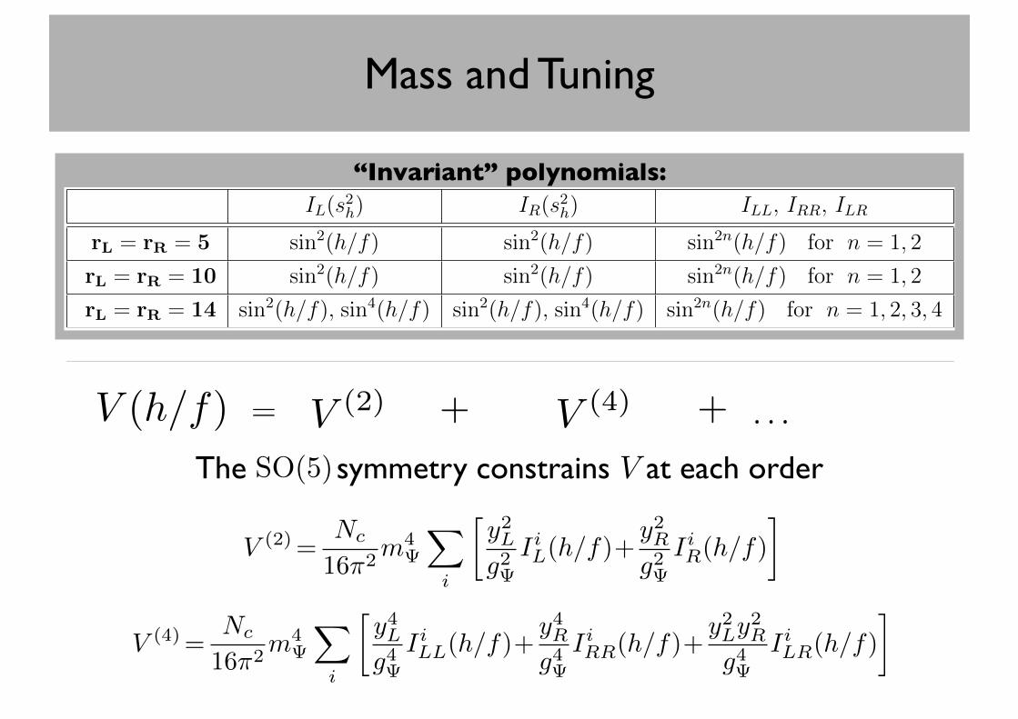
Higgs potential is radiatively generated
V (h/f) = V (2) + V (4) + . . .
The symmetry constrains at each orderSO(5) V
V (2)=Nc
16⇡2m4
X
i
y2Lg2
IiL(h/f)+y2Rg2
IiR(h/f)
�
V (4)=Nc
16⇡2m4
X
i
y4Lg4
IiLL(h/f)+y4Rg4
IiRR(h/f)+y2Ly
2R
g4 IiLR(h/f)
�
Mass and Tuning
V (h/f) = V (2) + V (4) + . . .
V
V (2)=Nc
16⇡2m4
X
i
y2Lg2
IiL(h/f)+y2Rg2
IiR(h/f)
�
V (4)=Nc
16⇡2m4
X
i
y4Lg4
IiLL(h/f)+y4Rg4
IiRR(h/f)+y2Ly
2R
g4 IiLR(h/f)
�
“Invariant” polynomials:
IL(s2h) ILL(s2h)
rL = 5 sin2(h/f) sin2n(h/f) with n = 1, 2
rL = 14 sin2(h/f), sin4(h/f) sin2n(h/f) with n = 1, 2, 3, 4
IL(s2h) IR(s2h) ILL, IRR, ILR
rL = rR = 5 sin2(h/f) sin2(h/f) sin2n(h/f) for n = 1, 2
rL = rR = 10 sin2(h/f) sin2(h/f) sin2n(h/f) for n = 1, 2
rL = rR = 14 sin2(h/f), sin4(h/f) sin2(h/f), sin4(h/f) sin2n(h/f) for n = 1, 2, 3, 4
rL = rR = 4 sin2(h/2f) sin2(h/2f) sin2n(h/2f) for n = 1, 2
Table 1: Table with all possible invariants appearing in the Higgs potential.
One caveat to eq. (9) is that in the limit of full compositeness, ✏R ⇠ 1 for the top right, there are nocontributions in ✏2R or ✏4R because the state is part of the strong sector respecting the global symmetries.In this case the y2t term in the second line of eq. (5) becomes of the same order of the formally leading✏2L because, as mentioned above, yL becomes of order yt. Indeed in the case of total tR compositenessthere is a single source of breaking of global symmetries, the mixing of the left doublet. Therefore theexpansion is truly in ✏2L. Another important remark is that the very notion of leading and subleadingterms becomes useless in the limit of very small fermionic coupling, g ⇠ yL,R because the expansionin ✏L,R looses its validity. In this case, similarly to what we mentioned below eq. (5) concerning theestimate of the Yukawa couplings, eq. (9) can be violated at O(1) but still it provides a valid estimateof the size of the Higgs potential.
3 Tuning and Mass of the Composite Higgs
The Higgs potential in eq. (9) generically has its minimum for hhi ⇠ f . The phenomenological successof the model requires instead hhi < f , i.e. that the famous parameter
⇠ =
✓v
f
◆2
= sin2
hhif
, (10)
is smaller than one. Reasonable values that give the model a chance to pass the EWPT are ⇠ = 0.2 or⇠ = 0.1. Achieving this requires unavoidably some cancellation. However the actual level of fine-tuning� which has to be enforced crucially depends on the structure of the Higgs potential, which in turn isdetermined by the choice of the fermionic representation and also by the size of the fermionic couplingg
. For what concerns the fine-tuning issue the composite Higgs models are conveniently classified intothree categories, which we will describe below. The popular MCHM
4
, MCHM5
and MCHM10
all belongto the first class and they su↵er of an enhanced (or “double”) amount of tuning. The tuning will besmaller in the other two categories, it will be of order
� = �min
=1
⇠. (11)
6
The symmetry constrains at each orderSO(5)
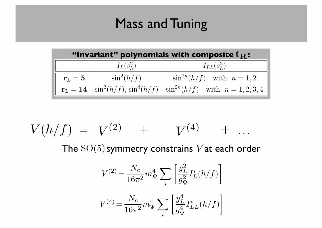
Mass and Tuning
V (h/f) = V (2) + V (4) + . . .
V
“Invariant” polynomials with composite :tR
V (4)=Nc
16⇡2m4
X
i
y4Lg4
IiLL(h/f)
�
V (2)=Nc
16⇡2m4
X
i
y2Lg2
IiL(h/f)
�
IL(s2h) ILL(s2h)
rL = 5 sin2(h/f) sin2n(h/f) with n = 1, 2
rL = 14 sin2(h/f), sin4(h/f) sin2n(h/f) with n = 1, 2, 3, 4
IL(s2h) IR(s2h) ILL, IRR, ILR
rL = rR = 5 sin2(h/f) sin2(h/f) sin2n(h/f) for n = 1, 2
rL = rR = 10 sin2(h/f) sin2(h/f) sin2n(h/f) for n = 1, 2
rL = rR = 14 sin2(h/f), sin4(h/f) sin2(h/f), sin4(h/f) sin2n(h/f) for n = 1, 2, 3, 4
rL = rR = 4 sin2(h/2f) sin2(h/2f) sin2n(h/2f) for n = 1, 2
Table 1: Table with all possible invariants appearing in the Higgs potential.
One caveat to eq. (9) is that in the limit of full compositeness, ✏R ⇠ 1 for the top right, there are nocontributions in ✏2R or ✏4R because the state is part of the strong sector respecting the global symmetries.In this case the y2t term in the second line of eq. (5) becomes of the same order of the formally leading✏2L because, as mentioned above, yL becomes of order yt. Indeed in the case of total tR compositenessthere is a single source of breaking of global symmetries, the mixing of the left doublet. Therefore theexpansion is truly in ✏2L. Another important remark is that the very notion of leading and subleadingterms becomes useless in the limit of very small fermionic coupling, g ⇠ yL,R because the expansionin ✏L,R looses its validity. In this case, similarly to what we mentioned below eq. (5) concerning theestimate of the Yukawa couplings, eq. (9) can be violated at O(1) but still it provides a valid estimateof the size of the Higgs potential.
3 Tuning and Mass of the Composite Higgs
The Higgs potential in eq. (9) generically has its minimum for hhi ⇠ f . The phenomenological successof the model requires instead hhi < f , i.e. that the famous parameter
⇠ =
✓v
f
◆2
= sin2
hhif
, (10)
is smaller than one. Reasonable values that give the model a chance to pass the EWPT are ⇠ = 0.2 or⇠ = 0.1. Achieving this requires unavoidably some cancellation. However the actual level of fine-tuning� which has to be enforced crucially depends on the structure of the Higgs potential, which in turn isdetermined by the choice of the fermionic representation and also by the size of the fermionic couplingg
. For what concerns the fine-tuning issue the composite Higgs models are conveniently classified intothree categories, which we will describe below. The popular MCHM
4
, MCHM5
and MCHM10
all belongto the first class and they su↵er of an enhanced (or “double”) amount of tuning. The tuning will besmaller in the other two categories, it will be of order
� = �min
=1
⇠. (11)
6
The symmetry constrains at each orderSO(5)
Mass and Tuning
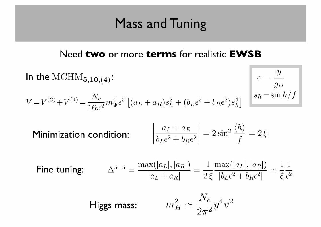
Need two or more terms for realistic EWSB
In the MCHM :MCHM5,10,(4)
V =V (2)+V (4)=Nc
16⇡2m4 ✏
2⇥(aL + aR)s
2h + (bL✏
2 + bR✏2)s4h
⇤
✏ =y
g sh=sinh/f
Minimization condition:
We refer to �min
= 1/⇠ as the “minimal tuning” because we expect that it provides the absolute lowerbound for the tuning required by any model of composite Higgs, for sure this is the case for all themodels of the present paper.
3.1 Double Tuning
As exhaustively discussed in [], a parametrically enhanced fine-tuning is needed in all the models wherea single invariant is present in the potential at the leading order in ✏L,R. In this case the subleadingterms must be taken into account in order to achieve a realistic EWSB. For instance for rL = rR = 5or 10 table 1 shows that the potential has the form1
V 5+5 = Vleading
+ Vsub�leading
=Nc
16⇡2
m4
✏2
⇥(aL + aR)s
2
h + (bL✏2 + bR✏
2)s4h⇤, (12)
where aL,R and bL,R are model-dependent O(1) numerical coe�cients. In the equation above we haveassumed, for simplicity, ✏L ' ✏R = ✏ = y/g , however nothing would be gained if relaxing this assump-tion. Indeed it is possible to show that the case yL ' yR discussed in the present section is the mostfavorable one, both the fine-tuning and the Higgs mass would increase for large separation yL ⌧ yR oryR ⌧ yL.
The tuning of the Higgs VEV, provided the signs of the coe�cients can be freely chosen, requires����
aL + aRbL✏2 + bR✏2
���� = 2 sin2
hhif
= 2 ⇠ . (13)
The amount of cancellation implied by the equation above is
�5+5 =max(|aL|, |aR|)
|aL + aR| =1
2 ⇠
max(|aL|, |aR|)|bL✏2 + bR✏2| ' 1
⇠
1
✏2, (14)
and it is parametrically larger than �min
for ✏ < 1. This accounts for the “double” tuning which has tobe performed on the potential (12): one must first cancel the ✏2 terms making them of the same orderof the formally subleading ✏4 ones, and afterwards further tune the ✏2 and ✏4 contributions. Once theminimization condition is imposed we can easily obtain the physical Higgs mass,
m2
H5+5
=8Ncg4 f
2
16⇡2
⇠(1� ⇠)✏4 (bL + bR) ' Nc
2⇡2
v2g4 ✏4 . (15)
The advantage of the doubly tuned models, which helps in obtaining a light Higgs boson, is that theHiggs quartic coupling is also automatically reduced in the tuning process. In spite of the fact that thepotential is generated at O(✏2) indeed the Higgs mass-term scales like ✏4 rather than ✏2.
However the reduction of mH is not su�cient for a 125 GeV Higgs, one extra ingredient is needed.Suppose indeed that we apply the naive estimate (5) for the top Yukawa. Since ✏L ' ✏R = ✏ we wouldobtain ✏ ' p
yt/g and therefore a too heavy Higgs
m5+5H '
rNc
2⇡2
y2t g2
v2 = 500GeV
⇣g 5
⌘. (16)
A realistic Higgs mass requires that we deviated from the estimate (5), and this occurs in the presenceof accidentally light fermionic states with the appropriate quantum numbers to mix strongly with the
1 Very similar consideration hold in the case rL = rR = 4, the only change is in the functional form of the leading andsubleading terms.
7
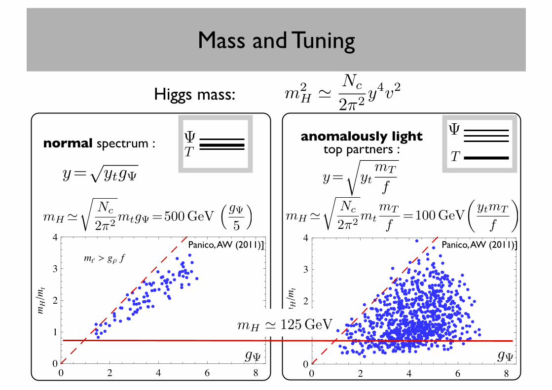
Fine tuning:
Higgs mass: m2H ' Nc
2⇡2y4v2
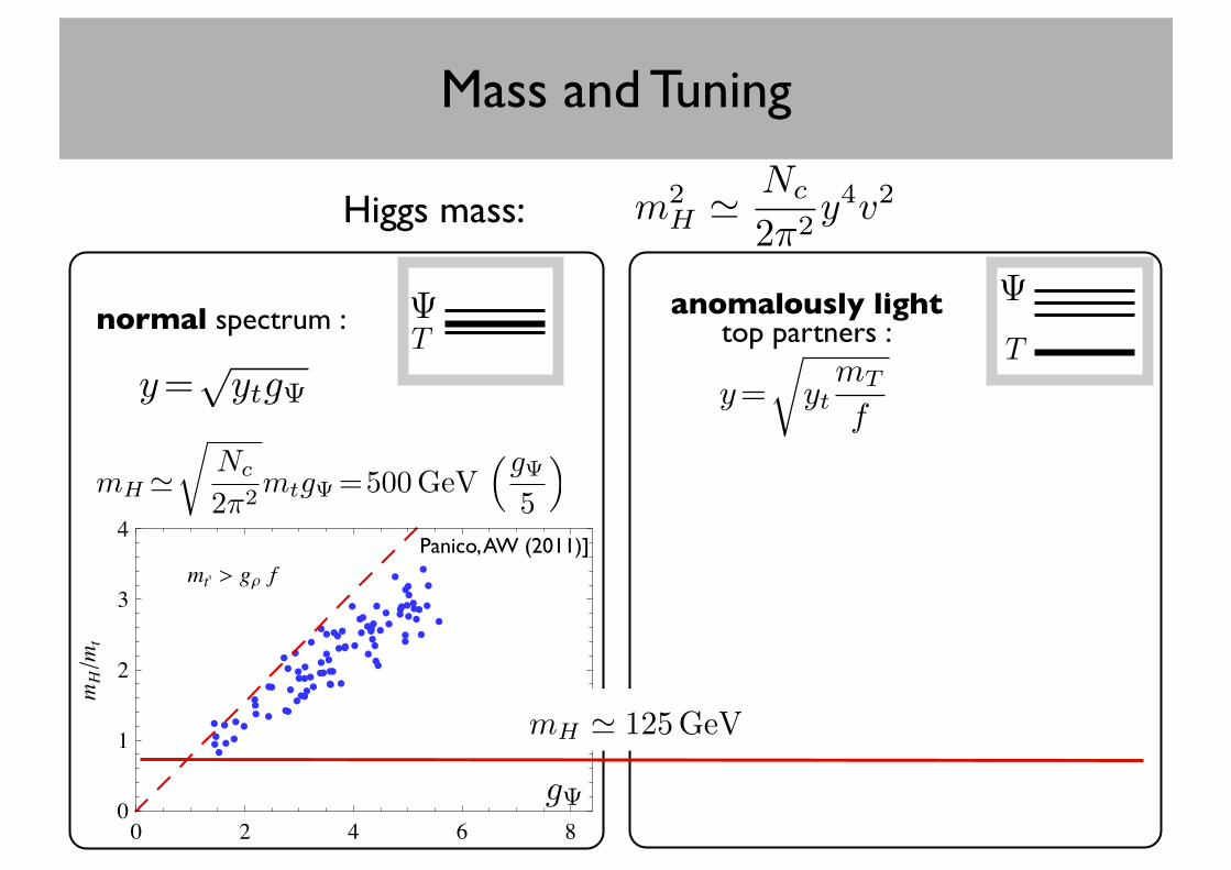
Mass and Tuning
Higgs mass: m2H ' Nc
2⇡2y4v2
T T
normal spectrum : anomalously light top partners :
y=pytg y=
rytmT
f
mH 'r
Nc
2⇡2mtg =500GeV
⇣g 5
⌘
Ë
Ë
Ë
ËË
Ë
Ë
ËË
ËË
Ë
Ë
ËË
Ë
Ë
Ë
Ë
Ë
Ë
ËË
Ë
ËË
Ë
Ë
Ë Ë
Ë
Ë
Ë
Ë
ËË
Ë
Ë
Ë
Ë
Ë
Ë
Ë
Ë
ËË
Ë
Ë
Ë
Ë
ËËËË
Ë
Ë
ËË
Ë
ËË
Ë
Ë
Ë
Ë
Ë
ËË
Ë
Ë
Ë
Ë
Ë
Ë
Ë
Ë Ë
Ë
ËË
Ë
ËË
Ë Ë
Ë
Ë
Ë
Ë
mt' > gr f
0 2 4 6 80
1
2
3
4
gr
mHêm t
g
Panico, AW (2011)]
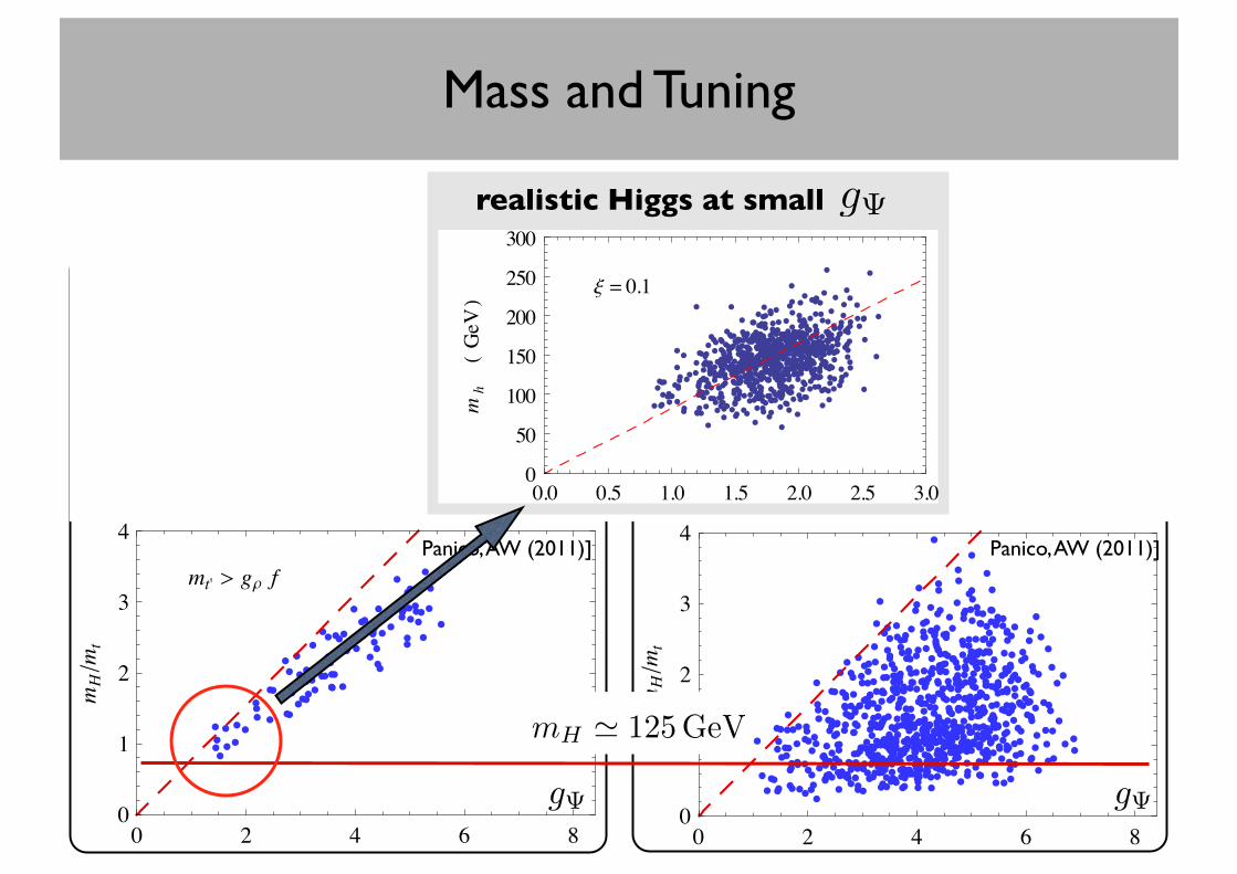
mH ' 125GeV
Mass and Tuning
Higgs mass: m2H ' Nc
2⇡2y4v2
Tnormal spectrum : anomalously light
top partners :
y=pytg y=
rytmT
f
mH 'r
Nc
2⇡2mtg =500GeV
⇣g 5
⌘mH '
rNc
2⇡2mt
mT
f=100GeV
✓ytmT
f
◆
Ë
Ë
Ë
ËË
Ë
Ë
ËË
ËË
Ë
Ë
ËË
Ë
Ë
Ë
Ë
Ë
Ë
ËË
Ë
ËË
Ë
Ë
Ë Ë
Ë
Ë
Ë
Ë
ËË
Ë
Ë
Ë
Ë
Ë
Ë
Ë
Ë
ËË
Ë
Ë
Ë
Ë
ËËËË
Ë
Ë
ËË
Ë
ËË
Ë
Ë
Ë
Ë
Ë
ËË
Ë
Ë
Ë
Ë
Ë
Ë
Ë
Ë Ë
Ë
ËË
Ë
ËË
Ë Ë
Ë
Ë
Ë
Ë
mt' > gr f
0 2 4 6 80
1
2
3
4
gr
mHêm t
ËË
Ë
ËË
Ë
Ë
ËË
Ë Ë
ËË ËËËË
Ë
Ë
Ë
Ë
Ë
ËË
Ë
ËË
ËË
Ë
Ë
Ë
Ë
ËË
Ë
Ë
Ë
ËË
ËË
Ë
Ë
Ë
Ë
Ë
Ë
Ë
ËË
Ë
Ë
Ë
Ë
Ë
Ë
Ë
ËË
Ë
Ë
ËË
Ë
ËËË
ËË
Ë
Ë
ËË
Ë
ËË
Ë
Ë
Ë
Ë
Ë
Ë
ËË
Ë
Ë
Ë
Ë
Ë
Ë
Ë
ËË
ËËË
Ë
Ë
ËË
Ë
ËË
Ë
Ë
ËË
Ë
Ë
Ë
ËË ËË
Ë
Ë
ËË
ËË
Ë
Ë
ËË
Ë
Ë
Ë
ËË
Ë
Ë
Ë
Ë
Ë
Ë
Ë ËË
Ë
ËË Ë
ËË
ËË
ËË
Ë
Ë
ËË
Ë
Ë
Ë
ËË
Ë
Ë Ë
Ë
Ë
Ë Ë
Ë
Ë
Ë
Ë Ë
Ë
Ë
Ë
ËË
ËË
Ë
Ë
Ë
Ë
Ë
ËË Ë
Ë
Ë
Ë
Ë
Ë Ë Ë
Ë
ËË
Ë
ËË
Ë
ËËË
ËË
Ë
Ë
ËËË Ë
Ë
ËË
Ë
Ë
Ë
Ë
Ë
ËË
Ë
Ë
ËË
Ë
Ë
ËË
Ë
Ë
Ë Ë
Ë
Ë
Ë
Ë
ËË
Ë
Ë
ËË
Ë
Ë
Ë
Ë
ËË
Ë
Ë
ËË
ËË
Ë
Ë Ë
Ë
Ë Ë
ËË
Ë
Ë
ËËË Ë
Ë
ËËË ËË
ËË
Ë
ËË
Ë
Ë
Ë
Ë
Ë
Ë
Ë
Ë
Ë ËË
Ë ËË
Ë Ë
Ë
ËË
ËË Ë
Ë
ËË
Ë
Ë
Ë
Ë
Ë
Ë
Ë
ËË
Ë Ë
Ë
ËË Ë
Ë
ËË
Ë
Ë
Ë
Ë ËË
Ë
Ë
Ë
Ë
Ë
Ë
Ë
ËË
Ë
Ë
Ë ËËË
Ë
Ë
Ë
Ë
Ë
ËË
Ë
Ë
Ë
Ë
Ë
Ë
Ë
Ë
Ë
Ë Ë
Ë
Ë
ËË
Ë
Ë
ËË
Ë
Ë
Ë
Ë
Ë
Ë
ËËË
Ë
Ë
ËË
Ë
ËË Ë
Ë
Ë
Ë
ËËË
Ë
Ë
ËË
ËË
Ë
ËË
Ë
ËËËË ËË
Ë
ËË
Ë
ËËË Ë
Ë
Ë
ËËË
Ë
Ë
Ë
Ë
Ë
Ë Ë
Ë
Ë
Ë
ËË
Ë
Ë
Ë
ËË
Ë
Ë
Ë
Ë
ËË
Ë
ËËË
Ë
Ë
Ë
Ë
Ë
Ë
Ë
ËËË
ËË
Ë
ËË
Ë
Ë
Ë
Ë
Ë
ËË
Ë
Ë
Ë ËË
Ë
Ë
Ë
Ë
ËË
Ë
Ë
ËËË
Ë
Ë
ËË
Ë
Ë
Ë
ËËË
ËË
Ë
Ë Ë
Ë
Ë
Ë
Ë
Ë
ËË
Ë
Ë
Ë
Ë
ËËË
Ë
Ë ËË
Ë
Ë Ë
Ë
Ë
Ë
Ë
Ë Ë
Ë
Ë
Ë
Ë
Ë
Ë
Ë
ËË
ËË
Ë
Ë
Ë
Ë
Ë
Ë
Ë Ë Ë
Ë
Ë
Ë
Ë
Ë
Ë
ËË
Ë
Ë
Ë
Ë ËË
ËË
Ë
ËË
ËË
Ë
Ë
ËË
ËË
Ë
Ë Ë
Ë
Ë
Ë
Ë
Ë Ë
ËË
Ë
ËË
ËË
Ë
Ë
Ë
Ë
Ë
Ë
Ë
Ë
Ë
Ë
ËËË
Ë
ËË
Ë
Ë
Ë
ËË
Ë
Ë
Ë Ë Ë
Ë
Ë
Ë
Ë
ËË
ËË
Ë
ËË
Ë
Ë
Ë
Ë
ËËË
Ë Ë
Ë
Ë
Ë
Ë
Ë
Ë
Ë
Ë
Ë
Ë
ËËË
ËËËË
Ë
Ë
Ë
Ë
Ë
Ë
Ë
ËËË Ë
ËËË
Ë
Ë
Ë
Ë
Ë
Ë
Ë
Ë
Ë
ËË
Ë
Ë
Ë
Ë Ë
Ë
Ë
Ë Ë
Ë
Ë
Ë
ËË Ë
Ë
Ë
Ë
Ë
Ë
Ë
Ë
Ë
ËË
Ë
Ë
ËË
Ë
ËË
Ë
Ë
ËËË
Ë
Ë
ËËË
ËË
Ë
Ë
ËË
ËË Ë
Ë
ËË
Ë
Ë
Ë
Ë
Ë
Ë
ËË
Ë
ËËË
Ë
ËË
Ë
Ë
Ë
Ë
Ë
Ë
ËËË
ËË
Ë
Ë
Ë
Ë
ËË
Ë
Ë
ËË
ËË Ë
Ë
Ë
ËË
ËË
ËË
Ë
ËËËË
ËË
Ë
Ë
ËË
ËË
ËË
Ë
ËËË
Ë
Ë
Ë
ËËË
Ë
Ë
Ë
Ë
Ë
Ë ËË
ËË
Ë
Ë
Ë
Ë Ë
ËË
Ë Ë
Ë
Ë
ËË
Ë
Ë
ËË
Ë
ËË
ËË
ËË ËËË
Ë
Ë
Ë
Ë
Ë Ë
Ë
ËË
Ë
Ë
Ë
Ë
Ë
Ë
Ë
Ë
Ë Ë
Ë
Ë
Ë
Ë
Ë
Ë
0 2 4 6 80
1
2
3
4
gr
mHêm t
g g
T
Panico, AW (2011)] Panico, AW (2011)]
mH ' 125GeV
Mass and Tuning
Higgs mass: m2H ' Nc
2⇡2y4v2
T
Tnormal spectrum :
anomalously light top partners :
y=pytg y=
rytmT
f
mH 'r
Nc
2⇡2mtg =500GeV
⇣g 5
⌘mH '
rNc
2⇡2mt
mT
f=100GeV
✓ytmT
f
◆
Ë
Ë
Ë
ËË
Ë
Ë
ËË
ËË
Ë
Ë
ËË
Ë
Ë
Ë
Ë
Ë
Ë
ËË
Ë
ËË
Ë
Ë
Ë Ë
Ë
Ë
Ë
Ë
ËË
Ë
Ë
Ë
Ë
Ë
Ë
Ë
Ë
ËË
Ë
Ë
Ë
Ë
ËËËË
Ë
Ë
ËË
Ë
ËË
Ë
Ë
Ë
Ë
Ë
ËË
Ë
Ë
Ë
Ë
Ë
Ë
Ë
Ë Ë
Ë
ËË
Ë
ËË
Ë Ë
Ë
Ë
Ë
Ë
mt' > gr f
0 2 4 6 80
1
2
3
4
gr
mHêm t
ËË
Ë
ËË
Ë
Ë
ËË
Ë Ë
ËË ËËËË
Ë
Ë
Ë
Ë
Ë
ËË
Ë
ËË
ËË
Ë
Ë
Ë
Ë
ËË
Ë
Ë
Ë
ËË
ËË
Ë
Ë
Ë
Ë
Ë
Ë
Ë
ËË
Ë
Ë
Ë
Ë
Ë
Ë
Ë
ËË
Ë
Ë
ËË
Ë
ËËË
ËË
Ë
Ë
ËË
Ë
ËË
Ë
Ë
Ë
Ë
Ë
Ë
ËË
Ë
Ë
Ë
Ë
Ë
Ë
Ë
ËË
ËËË
Ë
Ë
ËË
Ë
ËË
Ë
Ë
ËË
Ë
Ë
Ë
ËË ËË
Ë
Ë
ËË
ËË
Ë
Ë
ËË
Ë
Ë
Ë
ËË
Ë
Ë
Ë
Ë
Ë
Ë
Ë ËË
Ë
ËË Ë
ËË
ËË
ËË
Ë
Ë
ËË
Ë
Ë
Ë
ËË
Ë
Ë Ë
Ë
Ë
Ë Ë
Ë
Ë
Ë
Ë Ë
Ë
Ë
Ë
ËË
ËË
Ë
Ë
Ë
Ë
Ë
ËË Ë
Ë
Ë
Ë
Ë
Ë Ë Ë
Ë
ËË
Ë
ËË
Ë
ËËË
ËË
Ë
Ë
ËËË Ë
Ë
ËË
Ë
Ë
Ë
Ë
Ë
ËË
Ë
Ë
ËË
Ë
Ë
ËË
Ë
Ë
Ë Ë
Ë
Ë
Ë
Ë
ËË
Ë
Ë
ËË
Ë
Ë
Ë
Ë
ËË
Ë
Ë
ËË
ËË
Ë
Ë Ë
Ë
Ë Ë
ËË
Ë
Ë
ËËË Ë
Ë
ËËË ËË
ËË
Ë
ËË
Ë
Ë
Ë
Ë
Ë
Ë
Ë
Ë
Ë ËË
Ë ËË
Ë Ë
Ë
ËË
ËË Ë
Ë
ËË
Ë
Ë
Ë
Ë
Ë
Ë
Ë
ËË
Ë Ë
Ë
ËË Ë
Ë
ËË
Ë
Ë
Ë
Ë ËË
Ë
Ë
Ë
Ë
Ë
Ë
Ë
ËË
Ë
Ë
Ë ËËË
Ë
Ë
Ë
Ë
Ë
ËË
Ë
Ë
Ë
Ë
Ë
Ë
Ë
Ë
Ë
Ë Ë
Ë
Ë
ËË
Ë
Ë
ËË
Ë
Ë
Ë
Ë
Ë
Ë
ËËË
Ë
Ë
ËË
Ë
ËË Ë
Ë
Ë
Ë
ËËË
Ë
Ë
ËË
ËË
Ë
ËË
Ë
ËËËË ËË
Ë
ËË
Ë
ËËË Ë
Ë
Ë
ËËË
Ë
Ë
Ë
Ë
Ë
Ë Ë
Ë
Ë
Ë
ËË
Ë
Ë
Ë
ËË
Ë
Ë
Ë
Ë
ËË
Ë
ËËË
Ë
Ë
Ë
Ë
Ë
Ë
Ë
ËËË
ËË
Ë
ËË
Ë
Ë
Ë
Ë
Ë
ËË
Ë
Ë
Ë ËË
Ë
Ë
Ë
Ë
ËË
Ë
Ë
ËËË
Ë
Ë
ËË
Ë
Ë
Ë
ËËË
ËË
Ë
Ë Ë
Ë
Ë
Ë
Ë
Ë
ËË
Ë
Ë
Ë
Ë
ËËË
Ë
Ë ËË
Ë
Ë Ë
Ë
Ë
Ë
Ë
Ë Ë
Ë
Ë
Ë
Ë
Ë
Ë
Ë
ËË
ËË
Ë
Ë
Ë
Ë
Ë
Ë
Ë Ë Ë
Ë
Ë
Ë
Ë
Ë
Ë
ËË
Ë
Ë
Ë
Ë ËË
ËË
Ë
ËË
ËË
Ë
Ë
ËË
ËË
Ë
Ë Ë
Ë
Ë
Ë
Ë
Ë Ë
ËË
Ë
ËË
ËË
Ë
Ë
Ë
Ë
Ë
Ë
Ë
Ë
Ë
Ë
ËËË
Ë
ËË
Ë
Ë
Ë
ËË
Ë
Ë
Ë Ë Ë
Ë
Ë
Ë
Ë
ËË
ËË
Ë
ËË
Ë
Ë
Ë
Ë
ËËË
Ë Ë
Ë
Ë
Ë
Ë
Ë
Ë
Ë
Ë
Ë
Ë
ËËË
ËËËË
Ë
Ë
Ë
Ë
Ë
Ë
Ë
ËËË Ë
ËËË
Ë
Ë
Ë
Ë
Ë
Ë
Ë
Ë
Ë
ËË
Ë
Ë
Ë
Ë Ë
Ë
Ë
Ë Ë
Ë
Ë
Ë
ËË Ë
Ë
Ë
Ë
Ë
Ë
Ë
Ë
Ë
ËË
Ë
Ë
ËË
Ë
ËË
Ë
Ë
ËËË
Ë
Ë
ËËË
ËË
Ë
Ë
ËË
ËË Ë
Ë
ËË
Ë
Ë
Ë
Ë
Ë
Ë
ËË
Ë
ËËË
Ë
ËË
Ë
Ë
Ë
Ë
Ë
Ë
ËËË
ËË
Ë
Ë
Ë
Ë
ËË
Ë
Ë
ËË
ËË Ë
Ë
Ë
ËË
ËË
ËË
Ë
ËËËË
ËË
Ë
Ë
ËË
ËË
ËË
Ë
ËËË
Ë
Ë
Ë
ËËË
Ë
Ë
Ë
Ë
Ë
Ë ËË
ËË
Ë
Ë
Ë
Ë Ë
ËË
Ë Ë
Ë
Ë
ËË
Ë
Ë
ËË
Ë
ËË
ËË
ËË ËËË
Ë
Ë
Ë
Ë
Ë Ë
Ë
ËË
Ë
Ë
Ë
Ë
Ë
Ë
Ë
Ë
Ë Ë
Ë
Ë
Ë
Ë
Ë
Ë
0 2 4 6 80
1
2
3
4
gr
mHêm t
g g
mH ' 125GeV
realistic Higgs at small g
suggesting a lower value gbottom & 5 on the scale of the bottom partners in order to satisfy the exper-imental bounds. In our numerical analysis we will not impose a strict bound on the bottom partnermasses, but nevertheless we will give a preference to configuration with a sizable value of gbottom .
x = 0.1
0.0 0.5 1.0 1.5 2.0 2.5 3.00
50
100
150
200
250
300
gytop
mhHGe
VL x = 0.1
0.0 0.2 0.4 0.6 0.8 1.0 1.21
510
50100
500
m h ê m href
D
Figure 1: Scatter plots corresponding to ⇠ = 0.1. On the left Higgs mass as a function of g and onthe right plot showing the amount of tuning as a function of the deviation of the Higgs mass from thenaive estimate. The dashed red lines correspond the estimate given in eq. (??) and eq. (??). The scanshave been performed by randomly choosing the top partners mass parameters in the range [�3f⇡, 3f⇡]while the bottom partners mass paraneters have been chosen in the range [�10f⇡, 10f⇡]. The couplingof the gauge resonances has been fixed to the value g⇢ = 5. The top mass has been fixed to the valuemt = 150 GeV (see caption of fig. 3) and the bottom mass has been loosely fixed to the valuemb ' 4 GeVshould 2.5 GeV.
Let us now discuss quantitatively the properties of the Higgs mass and of the tuning in the presentset-up. As predicted by the estimates (see eq. (??)), the Higgs mass is relatively light and can easilytake values in the experimentally allowed region 115 GeV < mh < 130 GeV if the top patners are light(g . 2). This can be clearly seen from the scatter plot in fig. 1, where the Higgs mass is plotted as afunction of gtop . Moreover the amount of tuning is in good agreement with the estimate � ⇠ ⇠�1 as canbe inferred form the plots in fig. ??. One can see that the dependence of the tuning on the ratio betweenthe actual value of the Higgs mass and its estimate is still approximately valid, although a significantamount of spread is present.
In order to obtain a small Higgs a small value of g is preferred. A light Higgs can also be obtainedif some states are lighter than the overall scale as explained in the previous section but this comes atthe price of a larger tuning. Below we present a dedicated scan in the small g region. This is obtainedusing the results of [4].
4.2 Composite tR
As we discussed previously the model with tR composite can be realized coupling the left-handed fermionsto the 14. The new feature of this representation is that its decomposition under SO(4),
14 = 9+ 4+ 1 (48)
14
Panico, AW (2011)] Panico, AW (2011)]
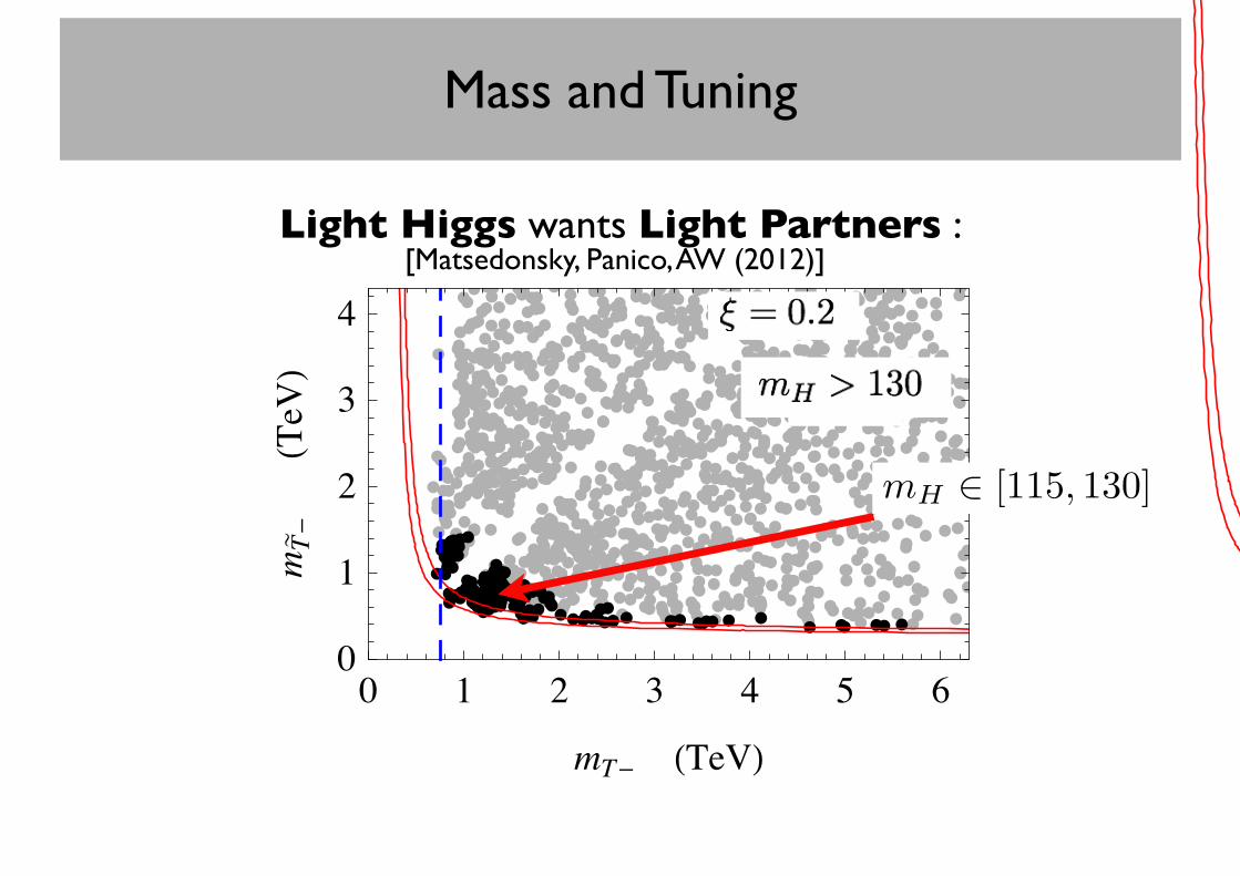
Mass and Tuning
Light Higgs wants Light Partners :
!"0.2
#
0 1 2 3 4 5 60
1
2
3
4
mT$ !TeV"
mT$
!TeV"
!"0.1
#
0 1 2 3 4 5 60
1
2
3
4
mT$ !TeV"
mT$
!TeV"
Figure 2: Scatter plots of the masses of the lightest T and eT resonances for ⇠ = 0.2 (left panel)
and ⇠ = 0.1 (right panel) in the three-site DCHM model. The black dots denote the points forwhich 115 GeV mH 130 GeV, while the gray dots have mH > 130 GeV. The scans have beenobtained by varying all the composite sector masses in the range [�8f, 8f ] and keeping the topmass fixed at the value mt = 150 GeV. The area between the solid red lines represents the rangeobtained by applying the result in eq. (44) for 115 GeV mH 130 GeV. The dashed blue linecorresponds to the estimate of the lower bound on mT� given in eq. (48).
The scatter plots of the masses of the T and eT light resonances are shown in fig. 2. One can
see that eq. (44) describes accurately the relation between the Higgs and the resonance masses in
the regions in which one state is significantly lighter than the others. For a realistic Higgs mass
this happens only when the eT� is much lighter than the other states. Instead, the situation of a
T much lighter than the eT can not happen for a light Higgs due to the presence of a lower bound
on the mT� , which will be discussed in details in the next section. In the region of comparable T�
and eT� masses sizable deviations from eq. (44) can occur. These are due to the possible presence
of a relatively light second level of resonances, as already discussed.
The numerical results clearly show that resonances with a mass of the order or below 1.5 TeV
are needed in order to get a realistic Higgs mass both in the case ⇠ = 0.2 and ⇠ = 0.1. The
prediction is even sharper for the cases in which only one state, namely the eT�, is light. In these
regions of the parameter space a light Higgs requires states with masses around 400 GeV for the
⇠ = 0.2 case and around 600 GeV for ⇠ = 0.1.
The situation becomes even more interesting if we also consider the masses of the other com-
posite resonances. As we already discussed, the first level of resonances contains, in addition to
the T� and eT�, three other states: a top-like state, the T
2/3�, a bottom-like state, the B�, and an
exotic state with charge 5/3, the X
5/3�. These three states together with the T� form a fourplet
20
mH � [115, 130]
[Matsedonsky, Panico, AW (2012)]
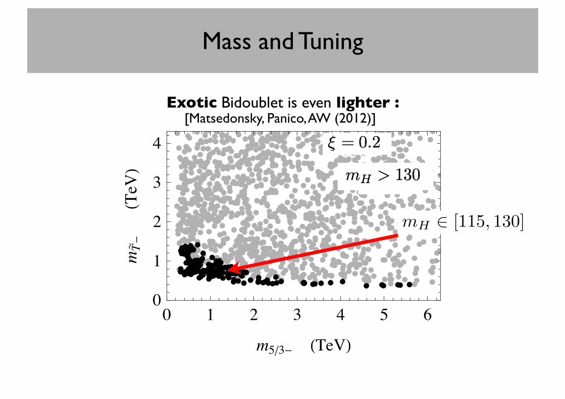
Mass and Tuning
!"0.2
#
0 1 2 3 4 5 60
1
2
3
4
m5!3$ "TeV#
mT$
"TeV#
!"0.1
#
0 1 2 3 4 5 60
1
2
3
4
m5!3$ "TeV#
mT$
"TeV#
Figure 3: Scatter plots of the masses of the lightest exotic state of charge 5/3 and of the lightesteT resonance for ⇠ = 0.2 (left panel) and ⇠ = 0.1 (right panel) in the three-site DCHM model.The black dots denote the points for which 115 GeV mH 130 GeV, while the gray dots havemH > 130 GeV. The scans have been obtained by varying all the composite sector masses in therange [�8f, 8f ] and keeping the top mass fixed at the value mt = 150 GeV.
of SO(4). Obviously the X
5/3� cannot mix with any other state even after EWSB, and therefore
it remains always lighter than the other particles in the fourplet. In particular (see fig. 9 for a
schematic picture of the spectrum), it is significantly lighter than the T� . In fig. 3 we show the
scatter plots of the masses of the lightest exotic charge 5/3 state and of the eT . In the parameter
space region in which the Higgs is light the X
5/3� resonance can be much lighter than the other
resonances, especially in the configurations in which the T� and eT� have comparable masses. In
these points the mass of the exotic state can be as low as 300 GeV.
Notice that in the plots in fig. 2 there are no points in which the masses of the T� and of the
eT� coincide. This is due to a repulsion of the mass levels induced by the mixings due to EWSB.
As expected, this e↵ect is more pronounced for larger values of ⇠.
3.4 The top mass and a lower bound on the Higgs mass
As noticed above, the asymptotic region mT� ⌧ meT�, which could in principle give rise to con-
figurations with realistic Higgs masses, is not accessible in our model. Indeed in the scatter plots
of fig. 2 we find a lower bound on mT�. We will show below that this bound comes from the
requirement of obtaining a realistic top mass and that an analogous bound, which however is not
visible in fig. 2, exists for the eT� mass. From these results we will also derive an absolute lower
bound on the Higgs mass.
21
Exotic Bidoublet is even lighter :
mH � [115, 130]
[Matsedonsky, Panico, AW (2012)]
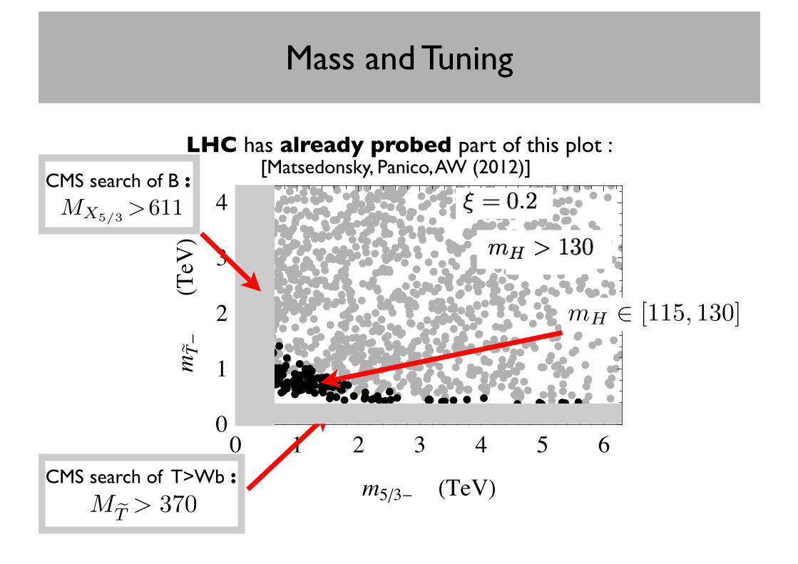
Mass and Tuning
LHC has already probed part of this plot :
CMS search of B :MX5/3
>611
!"0.2
#
0 1 2 3 4 5 60
1
2
3
4
m5!3$ "TeV#
mT$
"TeV#
!"0.1
#
0 1 2 3 4 5 60
1
2
3
4
m5!3$ "TeV#
mT$
"TeV#
Figure 3: Scatter plots of the masses of the lightest exotic state of charge 5/3 and of the lightesteT resonance for ⇠ = 0.2 (left panel) and ⇠ = 0.1 (right panel) in the three-site DCHM model.The black dots denote the points for which 115 GeV mH 130 GeV, while the gray dots havemH > 130 GeV. The scans have been obtained by varying all the composite sector masses in therange [�8f, 8f ] and keeping the top mass fixed at the value mt = 150 GeV.
of SO(4). Obviously the X
5/3� cannot mix with any other state even after EWSB, and therefore
it remains always lighter than the other particles in the fourplet. In particular (see fig. 9 for a
schematic picture of the spectrum), it is significantly lighter than the T� . In fig. 3 we show the
scatter plots of the masses of the lightest exotic charge 5/3 state and of the eT . In the parameter
space region in which the Higgs is light the X
5/3� resonance can be much lighter than the other
resonances, especially in the configurations in which the T� and eT� have comparable masses. In
these points the mass of the exotic state can be as low as 300 GeV.
Notice that in the plots in fig. 2 there are no points in which the masses of the T� and of the
eT� coincide. This is due to a repulsion of the mass levels induced by the mixings due to EWSB.
As expected, this e↵ect is more pronounced for larger values of ⇠.
3.4 The top mass and a lower bound on the Higgs mass
As noticed above, the asymptotic region mT� ⌧ meT�, which could in principle give rise to con-
figurations with realistic Higgs masses, is not accessible in our model. Indeed in the scatter plots
of fig. 2 we find a lower bound on mT�. We will show below that this bound comes from the
requirement of obtaining a realistic top mass and that an analogous bound, which however is not
visible in fig. 2, exists for the eT� mass. From these results we will also derive an absolute lower
bound on the Higgs mass.
21
mH � [115, 130]
CMS search of T>Wb :
MeT > 370
[Matsedonsky, Panico, AW (2012)]
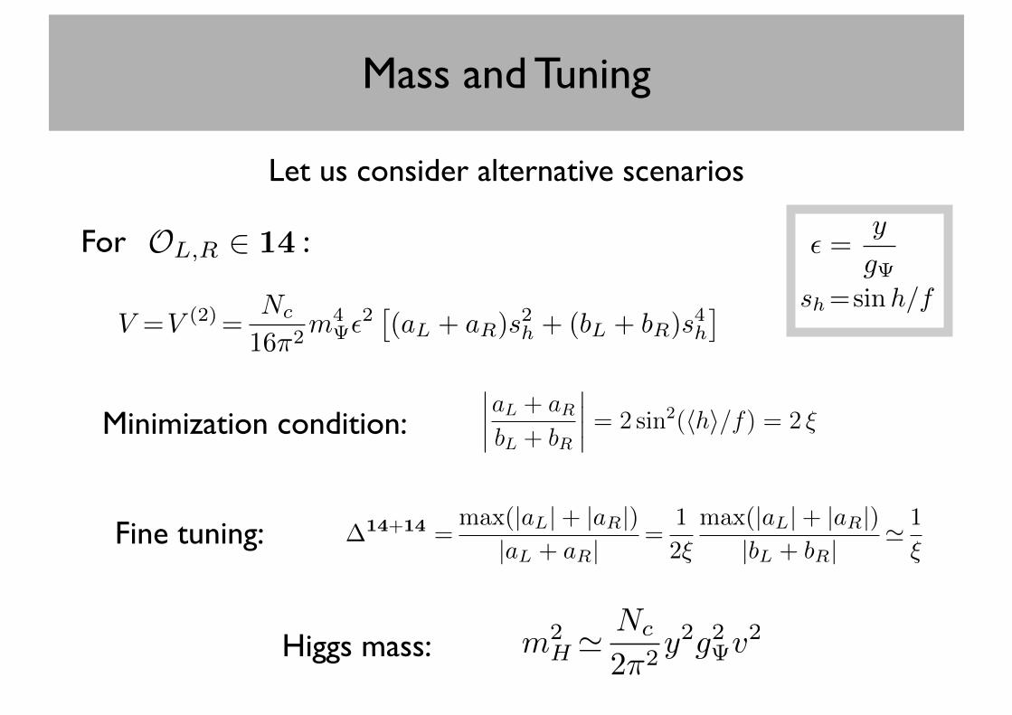
Mass and Tuning
Let us consider alternative scenarios
For MCHM : ✏ =y
g sh=sinh/f
Minimization condition:
Fine tuning:
Higgs mass:
OL,R 2 14
V =V (2)=Nc
16⇡2m4 ✏
2⇥(aL + aR)s
2h + (bL + bR)s
4h
⇤
top quark. In the cases of the 5+ 5 and of the 10+ 10 these states, the so-called top partners, are inthe 4 and/or in the singlet representation of SO(4). Given that the Yukawa couplings arise from themixing it is intuitive that their size will be controlled by the states that mix more strongly with the top.Indeed in the presence of anomalously light partners eq. (5) needs to be modified and becomes []
yt ' yLyRf
mp
. (17)
This estimates reduces to (5) if mp ' m = g f , but it can be parametrically di↵erent in the case of alarge separation mp < m . With the above equation and assuming yL ' yR we obtain y ' p
ytmp/fand therefore an Higgs mass
m5+5H '
rNc
2⇡2
ytmp
fv = 100GeV
✓ytmp
f
◆. (18)
A realistic Higgs is thus obtained if some of the top partners are light, at least below around 1 of 2 timesf , i.e. . 2 TeV.
No restriction is instead found on the overall scale m = g f of the other fermionic resonances. Aslong as the top partners are light a 125 GeV Higgs can be obtained even if m is large, indeed thismechanism is at work in the 5d holographic models where m is tight to m⇢ & 3 TeV. The price to pay,however, is a large tuning. Eq. (14) indeed becomes
�5+5 ' 1
⇠
g yt
m
mp
=1
⇠
rNc
2⇡2
g2 v
mH
=1
⇠· 20
✓125 GeV
mH
◆⇣g 5
⌘2
, (19)
and the tuning easily overcomes 100 for a realistic value of ⇠, below around 0.2.Notice that in the above discussion we have implicitly assumed the existence of a separation among
g and the elementary-composite couplings y, i.e. y < g . The situation is completely di↵erent if weinstead assume that all the fermionic couplings sector are of the same order, i.e. g ' y ' yt = 1. Inthis case all the terms in the e↵ective potential become equally large and the issue of double tuninggets nullified. Moreover a light Higgs becomes natural and there is no need to rely on anomalously lightpartners with specific quantum numbers. In this case all the fermionic resonances are generically light,with mass m ' f , we will consider an explicit model with these features in the following section.
3.2 Minimal Tuning
The issue of double tuning appears to be the result of an unfortunate coincidence and no much e↵ortis needed to avoid it. Indeed it is enough to chose the fermionic representations in such a way thattwo or more invariants are allowed in the leading order potential. Sticking to reducible representationsthe simplest choice is rL = rR = 14. Following Table 1 and again assuming ✏L ' ✏R the leading orderpotential has the form
V 14+14 = Vleading
=Nc
16⇡2
m4
✏2
⇥(aL + aR)s
2
h + (bL + bR)s4
h
⇤, (20)
and it can be adjusted to give a realistic EWSB without need of relying on the subleading terms. Theminimization condition is ����
aL + aRbL + bR
���� = 2 sin2(hhi/f) = 2 ⇠ , (21)
8�
14+14=
max(|aL|+ |aR|)|aL + aR|
=
1
2⇠
max(|aL|+ |aR|)|bL + bR|
' 1
⇠
m2H ' Nc
2⇡2y2g2 v
2
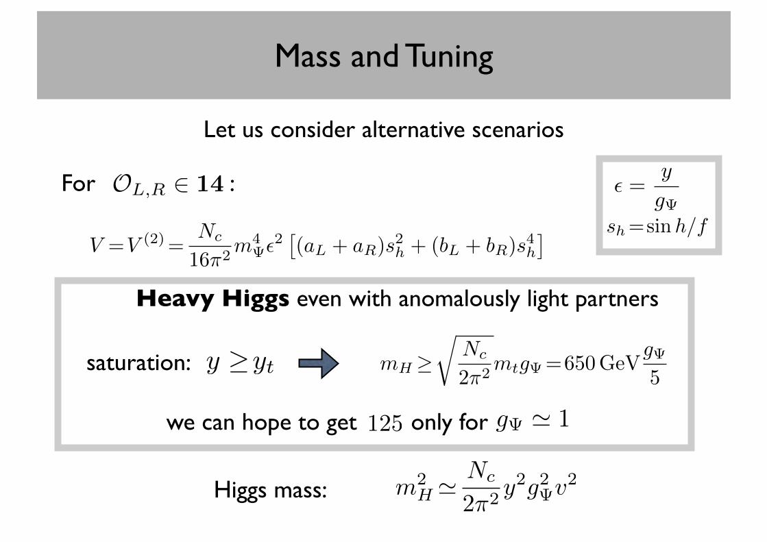
Mass and Tuning
Let us consider alternative scenarios
For MCHM : ✏ =y
g sh=sinh/f
Higgs mass:
OL,R 2 14
V =V (2)=Nc
16⇡2m4 ✏
2⇥(aL + aR)s
2h + (bL + bR)s
4h
⇤
m2H ' Nc
2⇡2y2g2 v
2
Heavy Higgs even with anomalously light partners
saturation: y �yt mH �r
Nc
2⇡2mtg =650GeV
g 5
we can hope to get only for 125 g ' 1
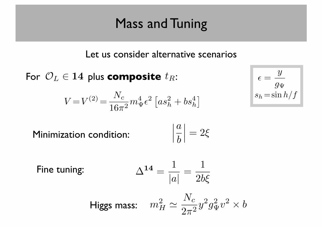
Mass and Tuning
Let us consider alternative scenarios
For MCHM plus composite : ✏ =y
g sh=sinh/f
Minimization condition:
Fine tuning:
Higgs mass:
tROL 2 14
V =V (2)=Nc
16⇡2m4 ✏
2⇥as2h + bs4h
⇤
���a
b
��� = 2⇠
�14 =1
|a| =1
2b⇠
m2H ' Nc
2⇡2y2g2 v
2 ⇥ b
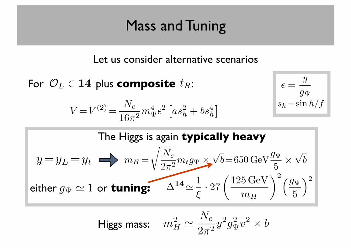
Mass and Tuning
Let us consider alternative scenarios
For MCHM plus composite : ✏ =y
g sh=sinh/f
Higgs mass:
tROL 2 14
V =V (2)=Nc
16⇡2m4 ✏
2⇥as2h + bs4h
⇤
The Higgs is again typically heavy
either or tuning:g ' 1
y=yL=yt mH =
rNc
2⇡2mtg ⇥
pb=650GeV
g 5
⇥pb
�14' 1
⇠· 27
✓125GeV
mH
◆2⇣g 5
⌘2
m2H ' Nc
2⇡2y2g2 v
2 ⇥ b
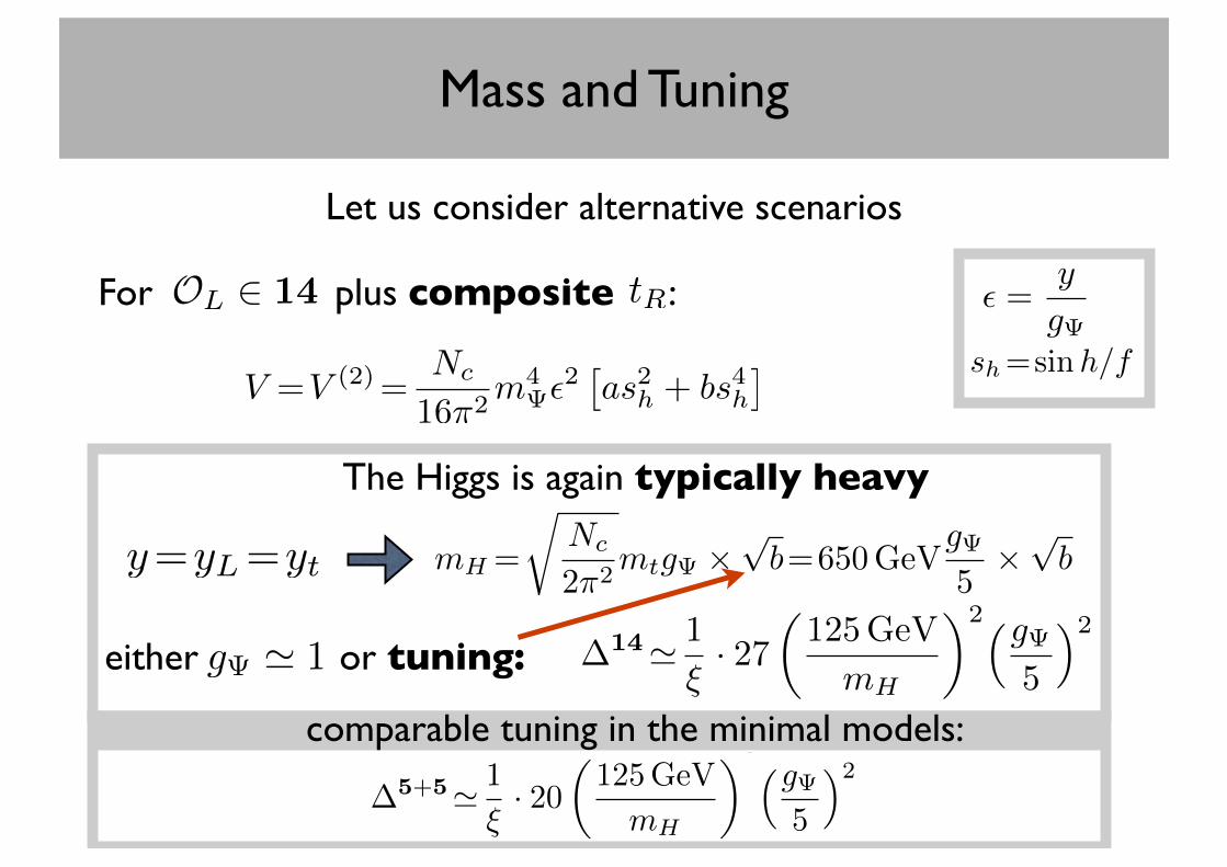
Mass and Tuning
Let us consider alternative scenarios
For MCHM plus composite : ✏ =y
g sh=sinh/f
tROL 2 14
V =V (2)=Nc
16⇡2m4 ✏
2⇥as2h + bs4h
⇤
either or tuning:g ' 1
y=yL=yt mH =
rNc
2⇡2mtg ⇥
pb=650GeV
g 5
⇥pb
comparable tuning in the minimal models:
�14' 1
⇠· 27
✓125GeV
mH
◆2⇣g 5
⌘2
�5+5' 1
⇠· 20
✓125GeV
mH
◆2⇣g 5
⌘2
The Higgs is again typically heavy
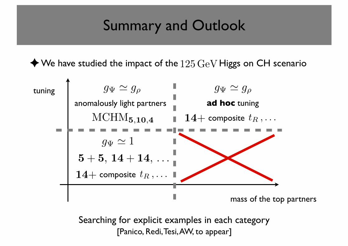
Summary and Outlook
✦ We have studied the impact of the Higgs on CH scenario125GeV
mass of the top partners
tuning
g ' 1
5+ 5, 14+ 14, . . .
14+ composite tR , . . .
g ' g⇢anomalously light partners
MCHM5,10,4
g ' g⇢ad hoc tuning
14+ composite tR , . . .
Searching for explicit examples in each category[Panico, Redi, Tesi, AW, to appear]
Summary and Outlook
✦ We have studied the impact of the Higgs on CH scenario
✦ Light top partners are typically required, essential for a moderate level of tuning
✦ Light partners are easily detectable, best way to search for CH !!
✦ Light partners could be in tension with EWPT is it really so in a concrete model ?
125GeV
[Barbieri, Bellazzini,Rychkov,Varagnolo (2012)]
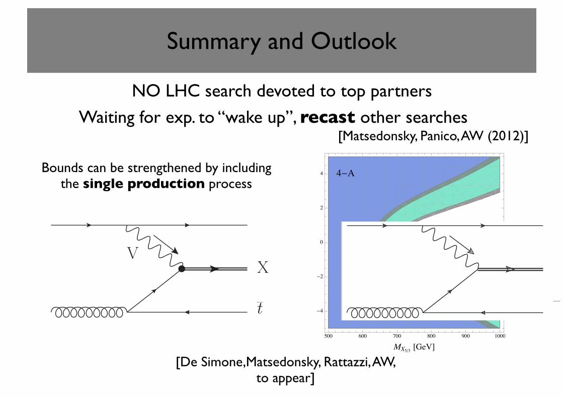
Summary and Outlook
NO LHC search devoted to top partners
Waiting for exp. to “wake up”, recast other searches[Matsedonsky, Panico, AW (2012)]
500 600 700 800 900 1000
-4
-2
0
2
4
MX5ê3 @GeVD
c 1
4-A
500 600 700 800 900 1000
-4
-2
0
2
4
MX5ê3 @GeVD
c 1
4-B
Figure 9: Excluded with 95%CL regions in the (MX
5/3
, c1
) plane for ⇠ = 0.2 for the models 4 -A and
4 -B : MB
� MX
5/3
(blue), MB
⇡ MX
5/3
(green). Gray regions correspond to the 30% variation of
the trilepton signal.
eT
The di↵erence of the models with a top partner in a singlet representation is that it can be single-
produced in association with a bottom quark and the corresponding cross section as it is shown on
the Fig. 3 is typically one order of magnitude higher than the pair production cross section in all
range of masses.
However the contribution of the eT produced in association with a b is almost eliminated by the
cuts applied in the Ref. [6]. The largest suppression e↵ect comes from the requirement to have at
least two jets and that RT
> 80GeV , where RT
is a sum of transverse momenta of all but two
highest pt
jets and all but two highest pt
leptons. These cuts are very tight since at the parton
level in this process we have only three charged leptons and tree jets two of which are typically very
forward. Hence even if one of the forward jets passes the jet pT
cut then the RT
cut becomes just a
requirement that minimal pt
of the charged leptons is higher than 80GeV .
Hence the signal events in the case of eT can come only from the single production in association
with a top quark and a pair production. And the bound on the cross section is also raised by the
sizable branching fractions of the eT decays to ht and Wb.
Plots and results
We show the cuts e�ciencies for the di↵erent types of production mechanisms in the Tab. 8 obtained
using the events samples produced with a MadGraph. As before the resulting e�ciencies include the
e↵ect of cuts, the branching ratios of vector bosons and a Higgs boson and identification e�ciencies
of di↵erent particles. Branching ratios of the top partners are not accounted for in the Tab. 8 but
note that in all cases to obtain desired final states at least one produced top partner must decay
26
[De Simone,Matsedonsky, Rattazzi, AW,to appear]
Bounds can be strengthened by including the single production process
t
XV
b
XV
Figure 2: The single production diagrams. (IMPROVE GRAPHICALLY)
with the bR
because the latter state is completely decoupled in our model, we expect this coupling
to be negligible even in more complete constructions.
It is important to outline that the couplings gXt
R
, gXt
L
and gXb
L
can be computed analytically in
our models. They arise from the interactions reported in Appendix B after performing the rotation
to the physical basis of mass eigenstates. Since the rotation matrices can be expressed in a closed
form the explicit formulas for the couplings are easily derived. The result is rather involved and for
this reason it will not be reported here, however it is easily implemented in a Mathematica package.
Once the couplings are known it is straightforward to obtain a semi-analytical formula for the
cross-sections of the single production processes, which can be parametrized as quadratic polynomials
in the couplings. The coe�cients will encapsulate the e↵ect of the QCD interactions, the integration
over the phase-space and the convolution with the parton distribution functions and they depend
uniquely on the mass of the partner. The production in association with the b is simply proportional
to g2Xb
L
while the one with t would be, a priori, the sum of three terms proportional to g2Xt
L
, g2Xt
R
and gXt
L
· gXt
R
which account, respectively, for the e↵ect of the left-handed coupling, of the right-
handed one and of the interference among the two. However in the limit of massless top quark,
mt
⌧ mX
, the processes mediated by the left-handed and by the right-handed couplings become
physically distinguishable because the anti-top produced in association with X will have opposite
chirality in the two cases. Therefore in the limit mt
! 0 the interference term can be neglected.
Moreover, the coe�cients of the gXt
L
2 and gXt
R
2 terms will be equal because the QCD interactions
are invariant under parity. Thus the cross-sections will be very simply parametrized as
�sing
(Xt) =1
2
h(g
Xt
L
)2 + (gXt
R
)2i�V t
(mX
) ,
�sing
(Xb) = (gXb
L
)2 �V b
(mX
) , (3.3)
in terms of few functions �V t
(mX
) and �V b
(mX
). The charge-conjugate processes, in which either
X t or X b are produced, can be parametrized in terms of the same functions because all what
matters for the calculation of the cross-section is the charge of the virtual V emitted from the light
quark line. Therefore we have
�sing
(Xt) =1
2
h(g
Xt
L
)2 + (gXt
R
)2i�V
†t
(mX
) ,
�sing
(Xb) = (gXb
L
)2 �V
†b
(mX
) , (3.4)
where V † denotes the charge conjugate of the vector boson V .
One might question the validity of the zero top mass approximation which allowed us to neglect
the interference and parametrize the cross-section as in eq.s (3.3) and (3.4). We might indeed
12
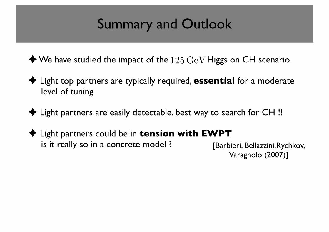
Summary and Outlook
✦ We have studied the impact of the Higgs on CH scenario
✦ Light top partners are typically required, essential for a moderate level of tuning
✦ Light partners are easily detectable, best way to search for CH !!
✦ Light partners could be in tension with EWPT is it really so in a concrete model ?
125GeV
[Barbieri, Bellazzini,Rychkov,Varagnolo (2007)]
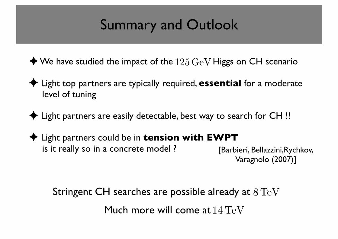
Stringent CH searches are possible already at !!8TeV
Much more will come at !14TeV
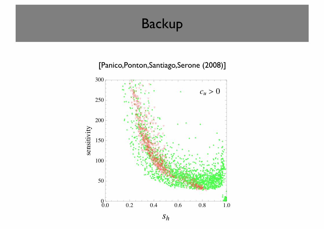
Backup
Figure 3: Left panel: logarithmic sensitivity as a function of sh
. Right panel: logarithmicsensitivity with the requirement that the top mass be kept fixed (see text). The green dotscorrespond to a random scan over parameter space with c
u
> 0. The subset that satisfies140 GeV < m
t
(µ ⇠ µIR
) < 160 GeV is indicated by red triangles. The results for the cu
< 0region are similar.
there is a sense in which there is little sensitivity to the details of the new physics beyond thestandard model. This also underscores the role that the heavy top plays in driving EWSB.
The above situation should be contrasted with supersymmetric (SUSY) scenarios thatalso present, generically, a sensitivity of order a percent to various fundamental parameters.In the SUSY case, reproducing a large top mass is no more di�cult than in the SM (it isenough to choose the top Yukawa coupling, one of the “fundamental” parameters of thesetheories, to be of order one). However, there is a well-known intrinsic fine-tuning associatedwith a cancellation between the µ term and the soft SUSY breaking parameters in the Higgssector. The latter depend quadratically on the stop soft SUSY breaking masses, which in turnneed to be taken somewhat heavy (at least in the simplest SUSY extensions of the standardmodel) in order to get a large enough Higgs quartic coupling that allows satisfying the LEPbound on the Higgs mass. If, in addition, one takes into account the RG running from a highscale, and quantifies the fine-tuning by the sensitivity to the high-energy parameters of thetheory, the situation worsens. In warped scenarios, the RS mechanism eliminates any possiblefine-tuning due to running from a high scale. The dynamical generation of the weak scale ingauge-Higgs unification scenarios, allows for a further natural separation between the weakscale and the KK scale µir. In fact, EWSB is generic, except that in most of parameter spaceit is characterized by s
h
= 1, which is not phenomenologically acceptable. The sensitivityshown in Fig. 3 is associated with the requirement 0 < s
h
< 1. Our observation is that allof this sensitivity is actually associated with getting the correct top mass (which in these
21
[Panico,Ponton,Santiago,Serone (2008)]