The Macroeconomics of Happiness - University of Warwick · The Macroeconomics of Happiness ......

The Macroeconomics of Happiness

Rafael Di TellaHarvard Business School

Robert J. MacCullochZEI, University of Bonn

and

Andrew J. OswaldUniversity of Warwick

December 28, 1998.

AbstractA large literature in macroeconomics assumes a social objective function,W(π, U), where inflation, π, and unemployment, U, enter negatively. Thispaper provides some of the first formal evidence for such an approach. Ituses cardinal data on reported well-being levels of approximately one-quarter of a million randomly sampled Europeans and Americans from the1970's to the 1990's. After controlling for personal characteristics, yeardummies, country fixed effects and country specific time trends we find thatthe data is correlated with inflation and unemployment. That is it traces outa W(π, U) function. These coefficients imply an inflation-unemploymenttrade off, and a dollar value of a low inflation rate. We use these cardinaldata to shed some light on an important hypothesis concerning the causes ofEuopean unemployment.

Keywords: Slope of social welfare functions, inflation-unemployment trade off.JEL Classification: E6

_________________________* Corresponding author: Rafael Di Tella, Morgan Hall, Soldiers Field, Boston, MA02163, USA. We thank Danny Blanchflower, Andrew Clark, Ben Friedman, GuillermoMondino, Julio Rotemberg and seminar participants at Oxford, Harvard, and the NBERBehavioral Macro Conference in 1998 for helpful discussions. The third author is gratefulto the Leverhulme Trust for research support.

2

I. Introduction

Modern macroeconomics textbooks rest upon the assumption of a social welfare function

defined on inflation, π, and unemployment, U.1 To our knowledge, no formal evidence on

the existence of such a function, W(π, U), has ever been presented in the literature.2

Instead the approach has become common because it is tractable and seems to accord

with what most politicians and some economists believe. Although an optimal policy rule

cannot be chosen unless the parameters of the presumed W(π, U) function are known,

that has not prevented the growth of a large theoretical literature in macroeconomics.

This paper tries to answer two questions we may want to ask about this approach.

First, we would like to know if people really care about these two variables. That is if

inflation and unemployment actually belong in the social welfare function. This is still an

important and debated question. A number of observers have charged that the industrial

democracies’ concern with price stability is excessive and wasteful.3 Second, we would

like to know how costly is inflation in terms of unemployment. That is what are the

weights attached to these variables in the social welfare function. In our attempt to

provide some answers to these two questions the paper uses cardinal data in the form of

answers to well being questions commonly used in the psychology literature. The data

come from random samples of individuals from many countries. Collected in standard

economic and social surveys, they provide self-reported cardinal measures of well being,

such as responses to questions about how happy and satisfied individual respondents are

with their lives.

By and large, economists are not interested in cardinal data like the response to

questions such as “Are you happy?” At least since Jevons, economists have noted that

cardinal statement from two persons, one saying that he is “very happy” and another

declaring herself “very unhappy”, imply nothing about their true levels of happiness. This

1 See, for example, Blanchard and Fischer (1989), Burda and Wyplosz (1993) andHall and Taylor (1993). Early influential papers include Barro and Gordon (1983).

2 Mankiw [1997] describes the question "How costly is inflation?" as one of the fourmajor unsolved problems of macroeconomics.

3

theoretical point put off the profession from analyzing cardinal measures ever since. But

surely the ultimate usefulness of cardinal data is an empirical matter. The paper reports

that well being equations (that regress individual cardinal responses on personal

characteristics of the individual) have remarkably similar structures across countries.

These equations, which play a fundamental role in our paper, are telling us that cardinal

data behave in a less erratic manner than what would justify the profession’s reluctance to

use cardinal data. Moreover, the patterns in these data seem - unknown to the respondents

completing their happiness score sheets - to trace out a W(π, U) function of the sort that

is assumed in the macroeconomics literature.4

Few economists have used data on reported well being. Easterlin (1974) began

what remains a fairly small literature. Recent contributions include Ng (1996) and Frank

(1985).5 Inglehardt (1990) XX

Largely the creation of Ronald Inglehardt, the Euro-Barometer Survey Series

records happiness and life satisfaction information on 300,000 people living in twelve

European countries over the period 1975 to the present. Section II presents the data and

suggests some reasons why such cardinal data may have useful information for

economists. Section III obtains a measure of the happiness in a particular year and

country that is not explained by the personal characteristics of the respondents. This

unexplained or residual macroeconomic happiness measure might be viewed as the

happiness on which government policy is supposed to focus. Using a panel analysis of

nations, we show that cardinal happiness data is correlated with inflation and

unemployment. This section also provides a measure that under some conditions can be

considered the inflation unemployment trade off that should guide macro policy.

In Section IV we explore a second application of our cardinal measure of well

being. Some economists have argued that the generous welfare state may be behind

Europe’s unemployment problems. By constructing separate measures of well being for

3 A recent contribution to this debate in the U.S. is Krugman's piece "Stable Prices andFast Growth: Just Say No", The Economist 31st August, 1996. 4 It may be useful to stress again that the analysis is not based on data asking peoplewhether they dislike inflation and unemployment. Our analysis complements the surveyapproach of, for example, Shiller (1996). 5 Kahneman, Wakker and Sarin (1997) provide an axiomatic defence of experiencedutility, and propose applications to economics.

4

the unemployed and for the employed, we are able to correlate a measure of generosity of

the unemployment benefit system with the happiness gap between the two groups. We

find some evidence that supports the economist’s received view on European

unemployment. Section V concludes.

II. Happiness Data

Data DescriptionThe U.S. data come from the United States General Social Survey [1972-1994].

Different individuals are interviewed each year and asked "Taken all together, how

would you say things are these days--would you say that you are very happy, pretty

happy, or not too happy?” The three relevant response categories for the later analysis are

"Very happy", "Pretty happy" and "Not too happy" (Small "Don't know" and "No

answer" categories are not included in our data set). The question was asked over 23

years to 26,668 individuals. Appendix I contains data sources and appendix II has the

data definitions.

The European data come from the Euro-Barometer Survey Series [1975-1991]. It

reports the answers to a similar happiness question and to a “life satisfaction” question.

This question, included in part because the word happy translates imprecisely across

languages, asks, "On the whole, are you very satisfied, fairly satisfied, not very satisfied

or not at all satisfied with the life you lead?” The four relevant response categories are:

"Very satisfied", "Fairly satisfied", "Not very satisfied" and "Not at all satisfied" (The

"Don't know" and "No answer" categories are not included in our data set). We focus on

life satisfaction data, as it is available for a longer period of time –from 1975 to 1991

instead of just 1975-86. Happiness and life satisfaction are correlated (the correlation

coefficient is 0.56 for the period 1975-86). The working paper version of this paper

presents some results using happiness data and some further estimates are available upon

request.

5

ValidationIn this sub-section we review some reasons why we may want to take happiness data

seriously. The first is a market-based argument: people who study well being for a living

(psychologists) actually used these data. Presumably, if there were better ways to study

well being, people who insist in using bad data would be driven out of the market. A

second, and perhaps more persuasive argument is that the data pass what psychologists

call validation exercises. For example, Pavot et al (1991) finds that people who report

themselves as very happy tend to smile more, an act that arguably is correlated with true

internal happiness. Also Diener (1984) finds that people who report themselves as very

happy tend to be rated by those around them as being relatively happy.

Third, it is possible to provide a validation check on the self-reported happiness

data used in the present paper using suicide data, provided suicides represent choices

made in response to extreme unhappiness. To test this idea, suicide rates were regressed

on country-by-year average reported life satisfaction, using the same panel of countries

used later in the paper. We controlled for year dummies and country fixed effects, and

corrected for heteroscedasticity using White's method. The regression evidence showed

that lower levels of reported well being are associated with higher suicide rates,

statistically significant at the 6 per cent level.

Finally, we study happiness and life satisfaction equations for individual

countries. The striking feature of this equations is that well being regressions seem to

share the same structure across countries. First we examine at micro-econometric

happiness equations for the U.S. and for the whole of Europe. These are ordered probit

equations that include a dummy for the country where the respondent lives and a dummy

for the year when the survey was carried out. Comparing the happiness equations for

Europe and the U.S., two features seem to stand out. The first is that the same personal

characteristics are statistically associated with happiness in Europe and the U.S.. Second,

the size of the effects does not vary much between the U.S. and Europe. For example, the

6

effect of employment status, being a widow and income (all three categories) is similar

across the U.S. and Europe. Blanchflower et al (1993) presents a similar micro-

econometric happiness regression for the U.S. between 1972 and 1990 with equivalent

results. Inglehardt XXX (Friedman). The following personal characteristics are positively

associated with happiness, and are statistically significant, in both Europe and the U.S.:

being employed, female, young or old (not middle aged), educated, married (neither

divorced, not separated nor a widow), with few children, or belonging to a high-income

quartile. Separate happiness regressions for each of the European countries largely repeat

these results. Being unemployed is associated with lower reported happiness levels in

every European country. The estimated effect in Spain where there is fewer data,

however, is not statistically significant at the 5% level.

Largely the same results obtain if we use life satisfaction data. Independent of the

country where the respondent lives, the same personal characteristics appear to be

important correlates with life satisfaction. These characteristics, in turn, work in the same

way as those in the happiness equations. Appendix III presents a micro-econometric life

satisfaction regression for Europe.

For every country in Europe, being unemployed increases the chance that the

respondent declares himself dissatisfied with life, even after holding other things constant

that may be expected to be associated with unemployment (e.g. family income, marital

separation). The size of the impact is large and similar across countries. With the

exception of Luxembourg, France and Greece, being unemployed is equivalent in life

dissatisfaction 'units' to dropping from the top to the bottom income quartile. For

Luxembourg the effect is almost double this, while in France an individual falling

unemployed is just as likely to report himself dissatisfied with his life as a person who

has experienced a drop in family income that takes him from the top to the second

income quartile. In Greece, unemployment is equivalent to a drop in family income from

the third to the bottom income quartile. While no definitive interpretation is possible, this

7

evidence is consistent with the common sense idea that unemployment is a major

economic source of human distress.

Males are more likely to declare themselves dissatisfied with their lives in most

countries. The exceptions are four Mediterranean countries: Italy, Portugal, Spain and

Greece. There is again evidence that life satisfaction is U-shaped in age, with the

coefficients similar across countries. The coefficient on self-employed is significantly

different from zero and negative in France, Italy, Spain, Portugal and Ireland. Married

individuals are more likely to report themselves satisfied with their lives in every country

except Portugal and France. Divorced individuals are more likely to report dissatisfaction

with their lives in every country except Spain and Ireland, which are two of the most

Catholic (and hence anti-divorce) countries in our sample. The only country where

separation is not associated with an increased chance of becoming more dissatisfied with

life is Spain and the only place where becoming a widow has a similar effect is Northern

Ireland. Having children (ages 8 to 15) tends to be associated with an increased chance

that the respondents are dissatisfied with life, although the effect is not always

statistically significant. Finally, for every country studied, having family income

classified in a higher income quartile increases the likelihood that a respondent is

satisfied with life. The effect is monotonic and the coefficients are similar across

countries.

III. Basic Inflation-Unemployment Trade Off in Happiness Equations

This section explores the basic macroeconomic trade off between inflation and

unemployment using life satisfaction and happiness data. A large literature in

macroeconomics assumes policy-makers maximise a social welfare function (minimise a

loss function) defined over a small number of variables of interest such as output,

unemployment and inflation. There is no agreement on the likely coefficients on these

8

variables or even if these variables belong to the social welfare function in the first place.

For example:

"we shall see that standard characterisations of the policy-maker's objective

function put more weight on the costs of inflation than is suggested by our

understanding of the effects of inflation; in doing so, they probably reflect

political realities and the heavy political costs of high inflation." (pp. 567-8,

Blanchard and Fischer (1987))

We study a regression of the form

ittiititit NTUNEMPLOYMEINFLATIONONSATISFACTILIFE µδεβα ++++=

where LIFE SATISFACTION is the average life satisfaction in country i in year t that is

not explained by personal characteristics. This is obtained by extracting the year

dummies from an OLS equation regressing life satisfaction on personal characteristics for

each of the countries covered.6 These dummies are our dependent variables.

UNEMPLOYMENT RATE is the unemployment rate in country i in year t, INFLATION

RATE is the rate of change of consumer prices in country i and year t, εi is a country fixed

effect, δt is a time effect (a year fixed effect and a time trend) and µit is an error term.

A two-step methodology is thus employed. In the first step, OLS life satisfaction

regressions on personal characteristics are estimated for each country in our sample. The

regressions combine a total of 270,150 observations. The mean residual life satisfaction is

then calculated for each year. In the second step, these country-by-year unexplained life

6 Using residuals from the probit regressions is not feasible. It introduces issues thathave not been resolved in the statistical literature. The use of OLS regressions has thewell-known problem that the data imply the distance between the categories verysatisfied and fairly satisfied is the same as the distance between the categories fairlysatisfied and not very satisfied. Experiments suggested to us that the precisecardinalization assumed did not alter the results. For example, a binary representation ofwell-being led to similar equations.

9

satisfaction components are used as the dependent variable in regressions of the form

given by the equation above. Three-year moving averages of the explanatory variables

are used.

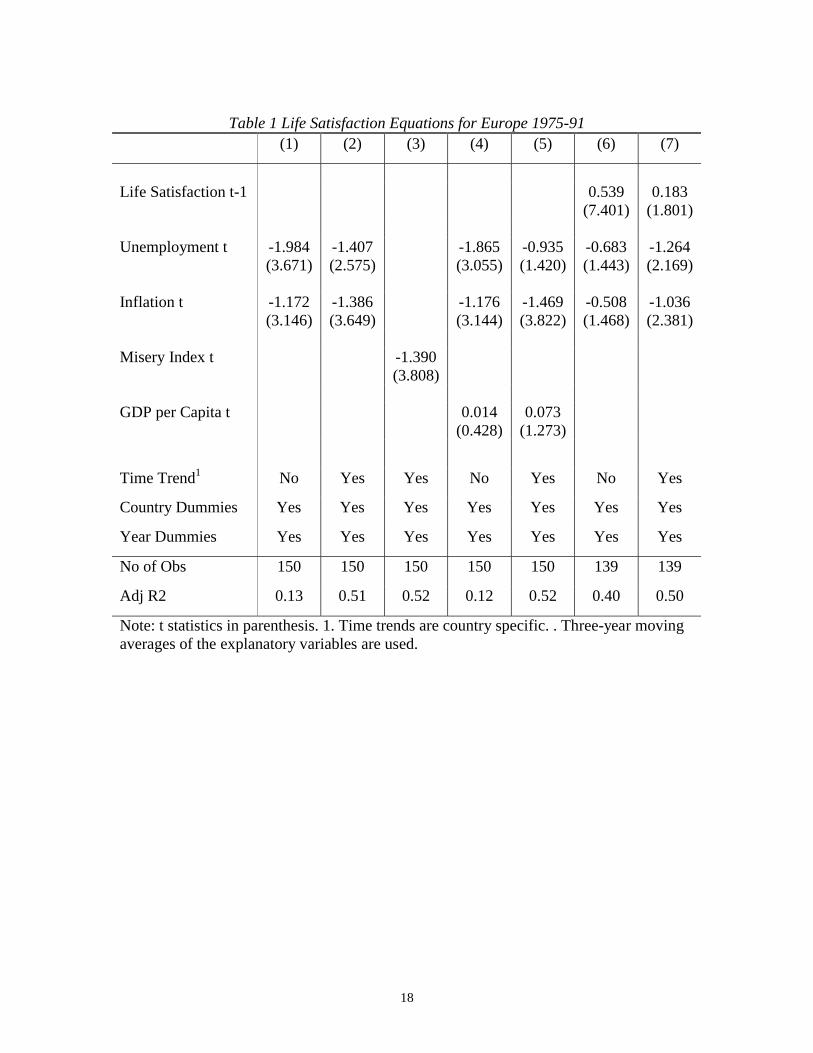
Table I presents the key empirical results. Regression (1) studies the dependence

of the life satisfaction residuals on the unemployment rate and the rate of inflation. The

specification includes time and country fixed effects. The coefficients from regression (1)

in Table I imply that higher unemployment and inflation rates decrease life satisfaction.

These coefficients are significant at the 1% level. In terms of the two questions the papers

sets out to answer, it seems that regression (1) indicates that both inflation and

unemployment belong to the social welfare function. And that our best guess regarding

the trade off between these variables is approximately equal to 1.7. That is, a country that

wishes to eradicate an inflation rate of 10% per annum is ready to bear a 6-percentage

point higher unemployment rate. Of course, in order to have a meaningful discussion

about a trade off we must make rather stark assumptions. For example, we must assume

that everybody is equal and that utility is linear (so that the margin is equal to the

average). A number of features of these numbers are also worth noting. First, this

calculation underestimates the cost of unemployment. Remember that we have already

controlled for the personal cost of being unemployed in the first stage regressions.

Regression (4) will suggest a simple way to correct for this. A second issue concerns the

temporal dimension of the data. By its nature, the data seem to be capturing instantaneous

happiness. Policy makers must then make their own calculations stating the number of

years that unemployment must be endured in order to obtain a given reduction in the

inflation rate.

Regression (2) in Table I shows that both unemployment and inflation enter

negatively and significantly after we introduce country specific time trends. The

coefficients on both variables are fairly similar, so that life satisfaction might be

reasonably well-approximated by a simple linear misery function, W=W(π+U).

10

Consequently, regression (3) explores the explanatory power of the variable, MISERY,

defined, as in the macroeconomic literature, as the linear addition of the inflation rate and

the unemployment rate. Higher levels of the misery index are associated with decreased

life satisfaction, an effect that is significant at the 1 per cent level.

Regression (4) of Table I repeats regression (1) and controls for the country’s

level of income per capita. Both inflation and unemployment are still negative and

significant though income is insignificant (but positive). Regression (5) repeats the

exercise including country specific time trends. The coefficients have the correct signs,

although those on unemployment and income are imprecisely estimated. One advantage

of these specifications is that it allows us to include the personal costs of unemployment

into the inflation unemployment trade off. From the micro regression (Table B in

appendix 3) we can get an estimate in terms of income of the personal costs of falling

unemployed. It seems that people who fall unemployed are approximately as happy as a

person who fall from the top to the bottom income quartile is. Taking mid points of these

quartiles implies a drop of U$6,670 in 1985 dollars. Thus, if we use the coefficients from

regression (5) we can see that a 1% unemployment rate leaves the average person equally

well off as a rise in the inflation rate from zero to 0.6%, or a receipt of U$129. This

ignores the personal costs of unemployment for the 1% who actually lost their jobs. This

would add on average U$66.70, or a third of a percentage point in the inflation rate.

(????)

This cost is significantly larger than the amounts calculated using the traditional

partial equilibrium approach, developed by Bailey (1956) and Friedman (1969), which

measures the welfare cost of inflation by computing the appropriate area under the money

demand curve. Using this method, Fischer (1981) and Lucas (1981) find the cost of

11

inflation to be surprisingly low, at 0.3 per cent and 0.45 per cent of national income,

respectively, for a 10 per cent level of inflation.7

Regressions (6) and (7) show that when the time trend is included either the

aggregate unemployment rate or the inflation rate in a country is a better predictor of the

level of well being than past levels of well being. Life satisfaction data seem to be

strongly correlated with macro variables.

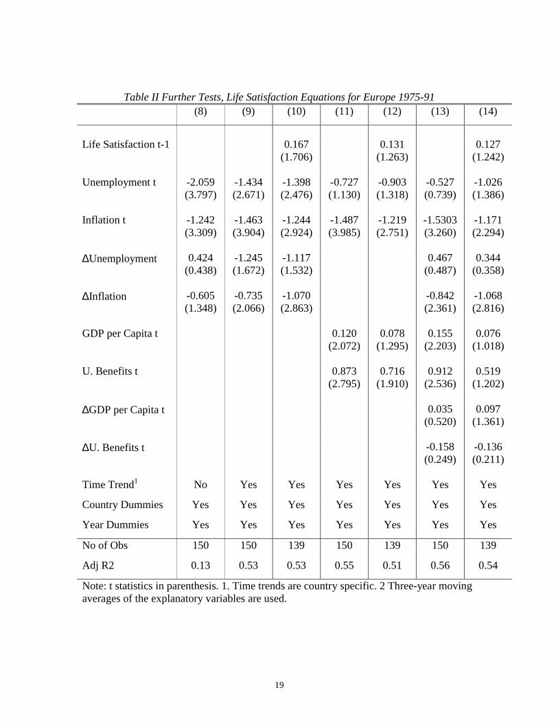
Table 2 presents some further tests regarding the relationship between inflation,

unemployment and well being. Regression (8) explores the hypothesis that well being

depends on the changes in our two macro variables. We use the change in inflation (or

unemployment) from one year to the next. There is little evidence that these changes

matter more than the levels. Including country specific time trends in regression (9)

somewhat changes this view as both changes enter with the expected sign and are

significant (the change in unemployment at the 10% level only). This is consistent with

the view that the variance of inflation is costly in terms of well being. Because these

measures of variability include changes in inflation from this year to the next, the

evidence is also consistent with the view that well being is forward looking. Regression

(10) shows that including a lagged dependent variable reinforces these findings.

We carried out some further tests (not reported but available upon request). We

studied the idea that high inflation has particularly high costs. Hence we included a

squared term for inflation. It shows that the coefficient on inflation becomes insignificant

once a term for inflation squared is included. The coefficient on the squared term, in turn,

is negative and significant at the 5% level. The result, however, does not survive the

inclusion of country specific time trends as it is again the level of inflation that enters

negative and significant in a well being equation. We also experimented with the idea

that unexpected inflation may have particularly high costs. We obtained a measure of

inflation forecasts made the previous year from the OECD Economic Outlook. We then

excluded inflation in year t and included this inflation forecast and the difference between

7 Before doing this analysis, we had shared the common economists' view that non-

12

actual inflation and this forecast (which may be presumed to capture unexpected inflation

levels). Controlling for country and year fixed effects, both expected inflation and

unexpected inflation entered negatively though the coefficient on the latter was

insignificant. Including country specific time trends turned the coefficient on unexpected

inflation larger in absolute value (more negative) than the coefficient on expected

inflation, and significant at the 4% level.

Our specification for what enters a social welfare function may be too restrictive.

Governments have explicit growth targets from year to year. And governments set up a

variety of safety nets that operate through the welfare state to cope with the uncertainties

of employment fluctuations. Regression (11) in Table II presents a specification that

includes GDP per Capita and a measure of the parameters of the unemployment benefit

system that has recently been compiled by the OECD. Although certainly superior to

previous measures of unemployment benefits used in the unemployment literature, the

data may still fail to capture a number of institutional features that affect the generosity of

the benefit system (e.g. the data does not capture the restrictions that make take up rates

vary so much across countries). Still we have confidence that this measure is correlated

with the hardship of life as an unemployed person in these countries. Both income and

benefits enter with the expected sign and are significant at conventional levels. The

unemployment rate is no longer significant however. Regression (12) includes a lagged

dependent variable and still finds significant effects of inflation and unemployment

benefits. Regression (13) and (14) presents very general specification with the level and

changes in these variables, with and without a lagged dependent variable. The basic result

is still that the coefficient on inflation and its change are negative and significant in

regressions explaining well being across countries.

Inflation, Unemployment and (Un)happiness in the United States

Since there is no question on life satisfaction in the United States General Social

Survey [1972-1994], it was not possible to include the US in the panel regressions.

economists over-estimate the cost of inflation.

13

However, there are GSS happiness data. We estimated an OLS happiness regression - not

reported - on personal characteristics for the U.S. and obtain the mean residuals for each

year. The year-to-year changes in the "(un)happiness residuals" (where higher values

indicate greater unhappiness) were positively correlated with the corresponding year-to-

year changes in the misery index. These yearly changes in unhappiness were more

strongly associated with changes in the unemployment rate than inflation. Figure 2 plots

the change in the residuals versus the change in unemployment, for the U.S. from 1972 to

1994, as an illustration of the analysis. Further details are available on request.

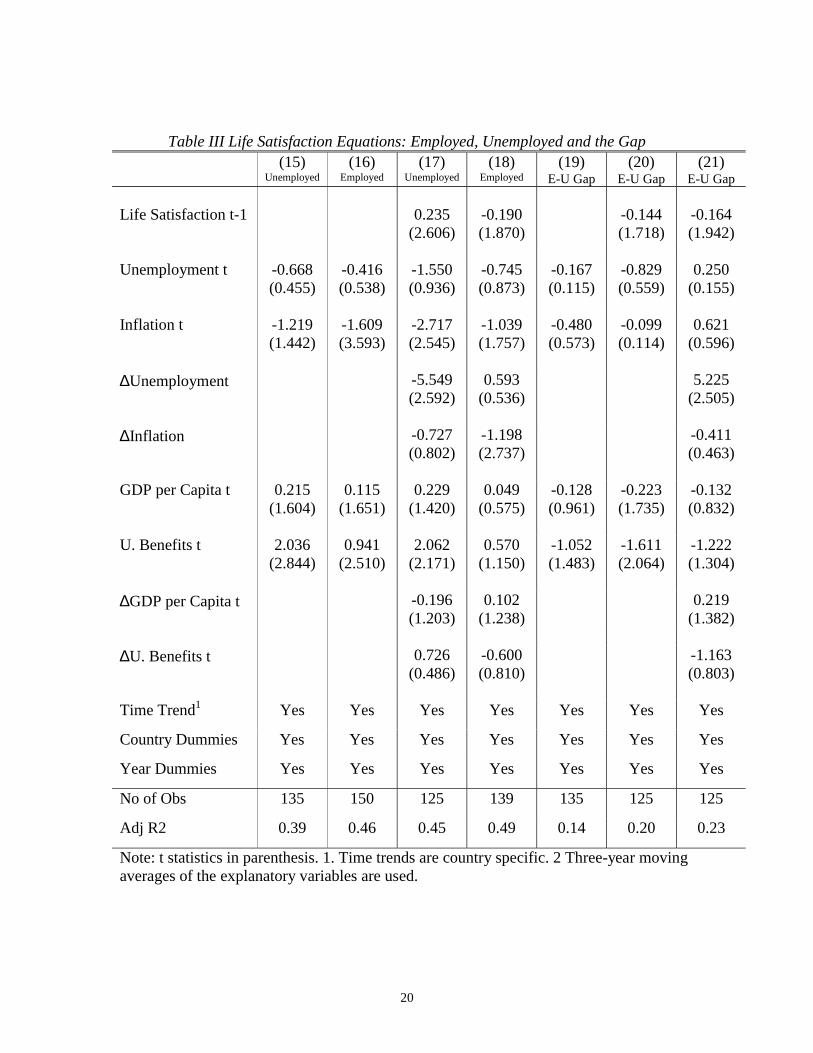
IV. Unemployed Well Being and Unemployment Benefits

The positive coefficient on unemployment benefits in all regressions in Table II is

intriguing. In order to shed some light on how unemployment benefits affect happiness

we divide our sample into unemployed and unemployed individuals. Regression (1) in

Table III studies the effect of inflation, unemployment, unemployment benefits and

income on the average residual life satisfaction of the unemployed. All variables enter

with the expected sign, though only benefits are significant. It is worth bearing in mind

that, because the unemployed are such a small fraction of the population, the average

number of respondents in each country and year is greatly reduced. Regression (15)

restricts attention to cell sizes greater or equal to 25. Thus, our confidence in these

estimates should be adjusted accordingly. As an example, note that if we consider cell

sizes greater than 15 observations, inflation become negative and significant. Re-

estimating regression (15) with robust regression techniques to reduce the influence of

outliers greatly increases the size of the coefficients on inflation (significant at the 1%

level) and unemployment (significant at the 7% level) to approximately equal sizes. The

coefficient on unemployment benefits is still large, positive and significant. Thus we

view these regressions as illustrative.

Regression (16) shows a similar life satisfaction regression for the employed.

Inflation and unemployment benefits enter with the expected signs and are well defined.

Comparing these results with those for the unemployed, the following three issues stand

14

out. First, the coefficient on the unemployment rate is insignificant. This is true even if

we re-estimate regression (16) with robust regression techniques. Furthermore it is

always smaller than the corresponding one in the regressions for the unemployed.

Second, inflation is negative and significant and larger in absolute size than that in

regression (15). It seems the employed care more about inflation than the unemployed.

Third, the coefficient on unemployment benefits in regression (16) is smaller than that in

regression (15). Regressions (17) and (18) present a more general specification. The

previous three findings are also true in these two regressions. Again we can see that

benefits affect more the happiness of the unemployed than the happiness of the

employed. An interesting fact is that the change in income has opposite signs in these two

regressions. Although imprecisely estimated (at the 23% level of significance in both

cases), it suggests that the unemployed are excluded from any income gains that may

occur in society.

Economists who study European unemployment have often claimed that generous

unemployment benefits make life too easy for the unemployed, leading to reduced work

incentives and higher unemployment rates. The previous regressions are certainly

consistent with this view. But we can explore this hypothesis further by taking the

difference between the average life satisfaction residuals of the employed and the

unemployed. We call this measure the happiness gap (E-U Gap). Regression (19) shows

how the happiness gap depends on our four macro variables. Unemployment benefits

enter negatively, though it is only significant at the 14% level. Re-estimating regression

(19) with robust regression techniques makes the coefficient on unemployment benefits

almost 70% larger and comfortably significant. Regression (20) shows that this is also the

case when we include a lag dependent variable. Regression (21) presents a very general

specification. Unemployment benefits are still negative, though no longer significant t

conventional levels. The effect of increases in the unemployment rate has a large,

positive and well-defined impact on the happiness gap. Increases in income are positive,

though not particularly well defined.8

15

V. Conclusions

We study well being data on a total of almost 300,000 people in twelve European

countries and the US. The data comes in the form of an answer to a simple question such

as “Are you happy?” The contributions of this paper are threefold.

First, and perhaps at a more general level, the paper shows that cardinal data is of

economic interest. At least since Jevons, economists have noted that cardinal statement

from two persons, one declaring himself “very happy” and another declaring herself

“very unhappy”, imply nothing about their true levels of happiness. This theoretical point

put off the profession from analysing cardinal measures. This paper shows that cardinal

measures have a remarkable amount of structure. The paper reports that well being

equations (that regress individual cardinal responses on personal characteristics of the

individual) have very similar structure across countries. These equations, which play a

fundamental role in our paper, are telling us that cardinal data behave in a less erratic

manner than what would justify the profession’s reluctance to use cardinal data.9

A second contribution is to show that macro variables matter. A large literature in

macroeconomics assumes the existence of a social welfare function of the form W(π, U).

To our knowledge, no evidence supporting this approach has been produced to this date.

And a number of observers have charged that the industrial democracies’ concern with

price stability is unwarranted and wasteful. We show that people, unknowingly, mark

lower numbers in their cardinal happiness scales at high inflation rates. The result that

inflation matters survives controlling for personal characteristics of the respondents,

country fixed effects, year fixed effects, country specific time trends, the inclusion of a

8 We also studied the impact of income inequality on happiness and life satisfaction.The data are insufficient for a proper test, but we found a little evidence that inequality ispositively correlated with social unhappiness. 9 Micro happiness equations are used to generate our second stage residuals, tovalidate our data and to incorporate the personal costs of falling unemployed into ourmacro trade-off.

16

lagged dependent variable, the inclusion of other variables such as income,

unemployment or unemployment benefits. It is worth remembering that people,

unknowingly, also mark lower numbers in their cardinal happiness scales when they live

on low-income levels. There is also some evidence that social happiness is negatively

correlated with the unemployment rate and positively correlated with the level of income

and the level of unemployment benefits.

The possibility of studying the correlates of such cardinal happiness measures

may be of importance for other questions besides that of whether inflation belongs in

W(π, U). For example, economists who study European unemployment claim that the

problem lies with the welfare state in these countries that makes life too easy for the

unemployed. We construct happiness cardinal measures for the employed and the

unemployed. We find that a measure of the generosity of the parameters of the

unemployment benefit system is more strongly (and positively) correlated with the

happiness of the unemployed. Thus we find some evidence for the claim that the Welfare

State reduces the happiness gap between the employed and the unemployed.

Third the paper presents some estimates of the inflation unemployment trade off

that is at the centre of much of modern macroeconomics. Although a number of

assumptions are needed have a more or less precise measure of the trade off the results

are of some interest. In a panel that controls for country fixed-effects and year effects

(year dummies and country specific time trends) our basic estimate suggests that people

would trade off a 1% inflation rate for an X% increase in the unemployment rate.

Including the personal costs of falling unemployed mean that the average person in

Europe a people is ready to see a Y% increase in the unemployment rate just to get rid of

a 1 percentage point in the inflation rate. We could also produce an income measure of

the inflation (or unemployment) costs. Although income is somewhat imprecisely

estimated our regression results indicate in 1985 US dollars, an inflation rate 1 percentage

point higher would have to be compensated by approximately $150 in extra income per

17

capita. Putting it differently, 1 percentage point of inflation corresponds to a well-being

cost of approximately 2 per cent of the level of income per capita.

18

Table 1 Life Satisfaction Equations for Europe 1975-91(1) (2) (3) (4) (5) (6) (7)

Life Satisfaction t-1 0.539(7.401)

0.183(1.801)

Unemployment t -1.984(3.671)

-1.407(2.575)

-1.865(3.055)

-0.935(1.420)

-0.683(1.443)

-1.264(2.169)

Inflation t -1.172(3.146)

-1.386(3.649)

-1.176(3.144)

-1.469(3.822)

-0.508(1.468)

-1.036(2.381)

Misery Index t -1.390(3.808)

GDP per Capita t 0.014(0.428)

0.073(1.273)

Time Trend1 No Yes Yes No Yes No Yes

Country Dummies Yes Yes Yes Yes Yes Yes Yes

Year Dummies Yes Yes Yes Yes Yes Yes Yes

No of Obs 150 150 150 150 150 139 139

Adj R2 0.13 0.51 0.52 0.12 0.52 0.40 0.50

Note: t statistics in parenthesis. 1. Time trends are country specific. . Three-year movingaverages of the explanatory variables are used.

19

Table II Further Tests, Life Satisfaction Equations for Europe 1975-91(8) (9) (10) (11) (12) (13) (14)


0.131(1.263)

0.127(1.242)


-1.434(2.671)

-1.398(2.476)

-0.727(1.130)

-0.903(1.318)

-0.527(0.739)

-1.026(1.386)


-1.463(3.904)

-1.244(2.924)

-1.487(3.985)

-1.219(2.751)

-1.5303(3.260)

-1.171(2.294)

∆Unemployment 0.424(0.438)

-1.245(1.672)

-1.117(1.532)

0.467(0.487)

0.344(0.358)

∆Inflation -0.605(1.348)

-0.735(2.066)

-1.070(2.863)

-0.842(2.361)

-1.068(2.816)


0.078(1.295)

0.155(2.203)

0.076(1.018)

U. Benefits t 0.873(2.795)

0.716(1.910)

0.912(2.536)

0.519(1.202)

∆GDP per Capita t 0.035(0.520)

0.097(1.361)

∆U. Benefits t -0.158(0.249)

-0.136(0.211)

Time Trend1 No Yes Yes Yes Yes Yes Yes



No of Obs 150 150 139 150 139 150 139

Adj R2 0.13 0.53 0.53 0.55 0.51 0.56 0.54

Note: t statistics in parenthesis. 1. Time trends are country specific. 2 Three-year movingaverages of the explanatory variables are used.

20

Table III Life Satisfaction Equations: Employed, Unemployed and the Gap(15)

Unemployed(16)

Employed(17)

Unemployed(18)

Employed(19)

E-U Gap(20)

E-U Gap(21)

E-U Gap


-0.190(1.870)

-0.144(1.718)

-0.164(1.942)


-0.416(0.538)

-1.550(0.936)

-0.745(0.873)

-0.167(0.115)

-0.829(0.559)

0.250(0.155)


-1.609(3.593)

-2.717(2.545)

-1.039(1.757)

-0.480(0.573)

-0.099(0.114)

0.621(0.596)

∆Unemployment -5.549(2.592)

0.593(0.536)

5.225(2.505)

∆Inflation -0.727(0.802)

-1.198(2.737)

-0.411(0.463)


0.115(1.651)

0.229(1.420)

0.049(0.575)

-0.128(0.961)

-0.223(1.735)

-0.132(0.832)

U. Benefits t 2.036(2.844)

0.941(2.510)

2.062(2.171)

0.570(1.150)

-1.052(1.483)

-1.611(2.064)

-1.222(1.304)

∆GDP per Capita t -0.196(1.203)

0.102(1.238)

0.219(1.382)

∆U. Benefits t 0.726(0.486)

-0.600(0.810)

-1.163(0.803)

Time Trend1 Yes Yes Yes Yes Yes Yes Yes



No of Obs 135 150 125 139 135 125 125

Adj R2 0.39 0.46 0.45 0.49 0.14 0.20 0.23

Note: t statistics in parenthesis. 1. Time trends are country specific. 2 Three-year movingaverages of the explanatory variables are used.

21

Appendix I

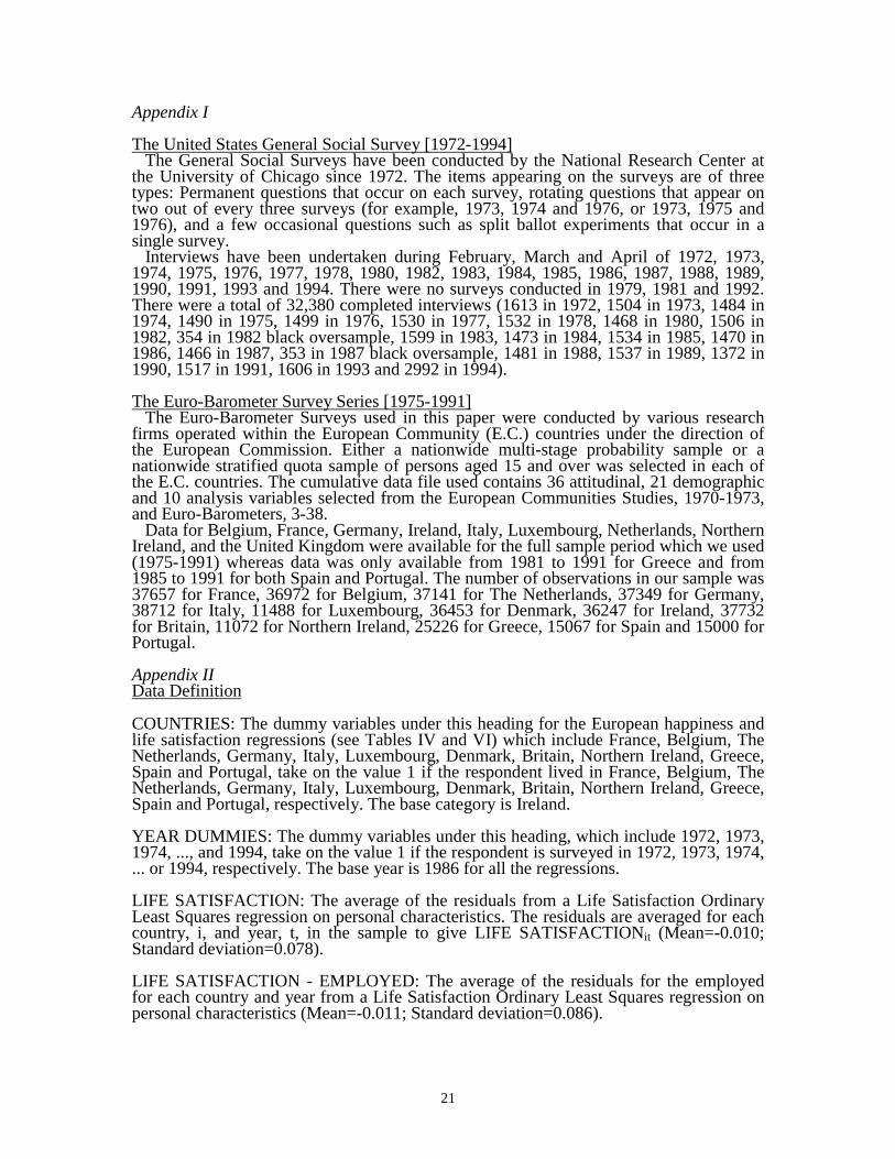
The United States General Social Survey [1972-1994] The General Social Surveys have been conducted by the National Research Center atthe University of Chicago since 1972. The items appearing on the surveys are of threetypes: Permanent questions that occur on each survey, rotating questions that appear ontwo out of every three surveys (for example, 1973, 1974 and 1976, or 1973, 1975 and1976), and a few occasional questions such as split ballot experiments that occur in asingle survey. Interviews have been undertaken during February, March and April of 1972, 1973,1974, 1975, 1976, 1977, 1978, 1980, 1982, 1983, 1984, 1985, 1986, 1987, 1988, 1989,1990, 1991, 1993 and 1994. There were no surveys conducted in 1979, 1981 and 1992.There were a total of 32,380 completed interviews (1613 in 1972, 1504 in 1973, 1484 in1974, 1490 in 1975, 1499 in 1976, 1530 in 1977, 1532 in 1978, 1468 in 1980, 1506 in1982, 354 in 1982 black oversample, 1599 in 1983, 1473 in 1984, 1534 in 1985, 1470 in1986, 1466 in 1987, 353 in 1987 black oversample, 1481 in 1988, 1537 in 1989, 1372 in1990, 1517 in 1991, 1606 in 1993 and 2992 in 1994).

The Euro-Barometer Survey Series [1975-1991] The Euro-Barometer Surveys used in this paper were conducted by various researchfirms operated within the European Community (E.C.) countries under the direction ofthe European Commission. Either a nationwide multi-stage probability sample or anationwide stratified quota sample of persons aged 15 and over was selected in each ofthe E.C. countries. The cumulative data file used contains 36 attitudinal, 21 demographicand 10 analysis variables selected from the European Communities Studies, 1970-1973,and Euro-Barometers, 3-38. Data for Belgium, France, Germany, Ireland, Italy, Luxembourg, Netherlands, NorthernIreland, and the United Kingdom were available for the full sample period which we used(1975-1991) whereas data was only available from 1981 to 1991 for Greece and from1985 to 1991 for both Spain and Portugal. The number of observations in our sample was37657 for France, 36972 for Belgium, 37141 for The Netherlands, 37349 for Germany,38712 for Italy, 11488 for Luxembourg, 36453 for Denmark, 36247 for Ireland, 37732for Britain, 11072 for Northern Ireland, 25226 for Greece, 15067 for Spain and 15000 forPortugal.

Appendix IIData Definition

COUNTRIES: The dummy variables under this heading for the European happiness andlife satisfaction regressions (see Tables IV and VI) which include France, Belgium, TheNetherlands, Germany, Italy, Luxembourg, Denmark, Britain, Northern Ireland, Greece,Spain and Portugal, take on the value 1 if the respondent lived in France, Belgium, TheNetherlands, Germany, Italy, Luxembourg, Denmark, Britain, Northern Ireland, Greece,Spain and Portugal, respectively. The base category is Ireland.

YEAR DUMMIES: The dummy variables under this heading, which include 1972, 1973,1974, ..., and 1994, take on the value 1 if the respondent is surveyed in 1972, 1973, 1974,... or 1994, respectively. The base year is 1986 for all the regressions.

LIFE SATISFACTION: The average of the residuals from a Life Satisfaction OrdinaryLeast Squares regression on personal characteristics. The residuals are averaged for eachcountry, i, and year, t, in the sample to give LIFE SATISFACTIONit (Mean=-0.010;Standard deviation=0.078).

LIFE SATISFACTION - EMPLOYED: The average of the residuals for the employedfor each country and year from a Life Satisfaction Ordinary Least Squares regression onpersonal characteristics (Mean=-0.011; Standard deviation=0.086).

22

LIFE SATISFACTION - UNEMPLOYED: The average of the residuals for theunemployed for each country and year from a Life Satisfaction Ordinary Least Squaresregression on personal characteristics (Mean=0.001; Standard deviation=0.158).

BENEFITS: The OECD index of (pre-tax) replacement rates (unemployment benefitentitlements divided by the corresponding wage, using a three year moving average). Incalculating this summary measure, the situation of a representative or average individualis estimated. Consequently, the unweighted mean of 18 numbers based on the followingscenarios is determined:-three unemployment durations (for persons with a long record of previous employment);the first year, the second and third years, and the fourth and fifth years of employment.-three family and income situations: a single person, a married person with a dependentspouse, and a married person with a spouse in work; and-two different levels of previous earnings: average earnings and two-thirds of averageearnings (For further details see the OECD Jobs Study [1994]).Since this index was calculated only for odd-numbered years, the value of BENEFITS foreven-numbered years was a linear interpolation (Mean=0.303; Standarddeviation=0.158).

UNEMPLOYMENT RATE: The unemployment rate (three year moving average) fromthe OECD Economic Outlook [1995] (Mean=0.087; Standard deviation=0.037).

INFLATION RATE: The inflation rate (three year moving average), as measured by therate of change in consumer prices, from IMF World Tables [1994] (Mean=0.086;Standard deviation=0.059).

GDP PER CAPITA: Real GDP per capita (three year moving average) at the price levelsand exchange rates of 1985 (U.S. dollars-measured in thousands), from OECD WorldStatistics [1993] (Mean=7606; Standard deviation=2402).

∆VR: For the corresponding variable, VR (measured as a three year moving average),∆VR measures the average change over the three year period.

23

References

Bailey, M. (1956). "The Welfare Cost of Inflationary Finance". Journal of PoliticalEconomy, 64-93.

Barro, R.J. and Gordon, D. (1983). "A Positive Theory of Monetary Policy in a NaturalRate Model", Journal of Political Economy, 91, 589-610.

Blanchard, O. and Fischer, S. (1989). Lectures on Macroeconomics, MIT Press,Cambridge.

Blanchflower, D., Oswald, A. J. and Warr, P. B. (1993). "Well Being Over Time inBritain and the USA", London School of Economics, Mimeo.

Burda, M. and Wyplosz, C. (1993). Macroeconomics: A European Text, OxfordUniversity Press, Oxford and New York.

Clark, A. and Oswald, A. J. (1994). "Unhappiness and Unemployment", The EconomicJournal, 104, 648-659.

Clark, A., Oswald, A. J. and Warr, P. B. (1996). "Is Job Satisfaction U-shaped in Age?",Journal of Occupational and Organizational Psychology, 69, 57-81.

Diener, E. (1984). "Subjective Well-Being", Psychological Bulletin, 93, 542-575.

Easterlin, R. (1974). "Does Economic Growth Improve the Human Lot? Some EmpiricalEvidence". In Nations and Households in Economic Growth: Essays in Honour ofMoses Abramovitz, (ed. P. A. David and M. W. Reder). New York and London:Academic Press.

Easterlin, R. (1995). "Will Raising the Incomes of All Increase the Happiness of All?",Journal of Economic Behaviour and Organization, 27, 35-48.

Fischer, S. (1981). "Towards an Understanding of the Costs of Inflation: II, Carnegie-Rochester Conference Series on Public Policy, 15, 5-41.

Frank, R. H. (1985). Choosing the Right Pond, Oxford University Press, New York andOxford.

Friedman, M. (1969). "The Optimum Quantity of Money", The Optimum Quantity ofMoney and Other Essays, Aldine, Chicago.

Hall, R. E. and Taylor, J.B. (1993). Macroeconomics (4th Edition), Norton, New York.

Inglehardt, R. (XX)

Kahneman, D., Wakker, P.P. and Sarin, R. (1997). "Back to Bentham? Explorations ofExperienced Utility", Quarterly Journal of Economics, 112, 357-406.

Lucas, R. E., Jr. (1981). "Discussion of: Stanley Fischer, 'Towards an Understanding ofthe Costs of Inflation: II", Carnegie-Rochester Conference Series on PublicPolicy, 15, 43-52.

Mankiw, N. G. (1997). Macroeconomics (3rd Edition), Worth Publishers, New York.

Ng, Y-K. (1996). "Happiness Surveys: Some Comparability Issues and an ExploratorySurvey Based on Just Perceivable Increments", Social Indicators Research, 38, 1-27.

24

OECD (1994). The OECD Jobs Study, OECD.

Oswald, A.J. (1997). "Happiness and Economic Performance", Economic Journal,forthcoming.

Pavot, W. (1991). "Further Validation of the Satisfaction with Life Scale: Evidence forthe Cross-Method Convergence of Well-Being Measures", Journal of PersonalityAssessment, 57, 149-161.

Shiller, R. (1996). "Why Do People Dislike Inflation?", National Bureau of EconomicResearch Working Paper, #5539.

The Macroeconomics of Happiness - University of Warwick · The Macroeconomics of Happiness ......

Documents

Transcript of The Macroeconomics of Happiness - University of Warwick · The Macroeconomics of Happiness ......