The Lorenz system

James Hateley

Contents

1 Formulation 2

2 Fixed points 4

3 Attractors 4

4 Phase analysis 54.1 Local Stability at The Origin . . . . . . . . . . . . . . . . . . . . . . . . . . . . . . . . . . . . 54.2 Global Stability . . . . . . . . . . . . . . . . . . . . . . . . . . . . . . . . . . . . . . . . . . . . 6

4.2.1 0 < ρ < 1 . . . . . . . . . . . . . . . . . . . . . . . . . . . . . . . . . . . . . . . . . . . 64.2.2 1 < ρ < ρh . . . . . . . . . . . . . . . . . . . . . . . . . . . . . . . . . . . . . . . . . . 6

4.3 Bifurcations . . . . . . . . . . . . . . . . . . . . . . . . . . . . . . . . . . . . . . . . . . . . . . 64.3.1 Supercritical pitchfork bifurcation: ρ = 1 . . . . . . . . . . . . . . . . . . . . . . . . . 74.3.2 Subcritical Hopf-Bifurcation: ρ = ρh . . . . . . . . . . . . . . . . . . . . . . . . . . . . 8

4.4 Strange Attracting Sets . . . . . . . . . . . . . . . . . . . . . . . . . . . . . . . . . . . . . . . 84.4.1 Homoclinic Orbits . . . . . . . . . . . . . . . . . . . . . . . . . . . . . . . . . . . . . . 94.4.2 Poincare Map . . . . . . . . . . . . . . . . . . . . . . . . . . . . . . . . . . . . . . . . . 94.4.3 Dynamics at ρ∗ . . . . . . . . . . . . . . . . . . . . . . . . . . . . . . . . . . . . . . . . 94.4.4 Asymptotic Behavior . . . . . . . . . . . . . . . . . . . . . . . . . . . . . . . . . . . . . 104.4.5 A Few Remarks . . . . . . . . . . . . . . . . . . . . . . . . . . . . . . . . . . . . . . . . 10

5 Numerical Simulations and Figures 105.1 Globally stable , 0 < ρ < 1 . . . . . . . . . . . . . . . . . . . . . . . . . . . . . . . . . . . . . . 105.2 Pitchfork Bifurcation, ρ = 1 . . . . . . . . . . . . . . . . . . . . . . . . . . . . . . . . . . . . . 125.3 Homoclinic orbit . . . . . . . . . . . . . . . . . . . . . . . . . . . . . . . . . . . . . . . . . . . 125.4 Transient Chaos . . . . . . . . . . . . . . . . . . . . . . . . . . . . . . . . . . . . . . . . . . . 125.5 Chaos . . . . . . . . . . . . . . . . . . . . . . . . . . . . . . . . . . . . . . . . . . . . . . . . . 14

5.5.1 A plot for ρh . . . . . . . . . . . . . . . . . . . . . . . . . . . . . . . . . . . . . . . . . 145.6 Other Notable Orbits . . . . . . . . . . . . . . . . . . . . . . . . . . . . . . . . . . . . . . . . 16

5.6.1 Double Periodic Orbits . . . . . . . . . . . . . . . . . . . . . . . . . . . . . . . . . . . 165.6.2 Intermittent Chaos . . . . . . . . . . . . . . . . . . . . . . . . . . . . . . . . . . . . . . 165.6.3 A Periodic Orbit . . . . . . . . . . . . . . . . . . . . . . . . . . . . . . . . . . . . . . . 18

6 MATLAB Code 186.1 LORENZ.m: . . . . . . . . . . . . . . . . . . . . . . . . . . . . . . . . . . . . . . . . . . . . . 186.2 LORENZ SYS.M . . . . . . . . . . . . . . . . . . . . . . . . . . . . . . . . . . . . . . . . . . . 206.3 LORENZ SYS VEC.M . . . . . . . . . . . . . . . . . . . . . . . . . . . . . . . . . . . . . . . . 216.4 PLOTTING SCRIPT.M . . . . . . . . . . . . . . . . . . . . . . . . . . . . . . . . . . . . . . . 21

Bibliography 25

1

THE LORENZ SYSTEM 1 FORMULATION

1 Formulation

The Lorenz system was initially derived from a Oberbeck-Boussinesq approximation. This approximation isa coupling of the Navier-Stokes equations with thermal convection. The original problem was a 2D problemconsidering the thermal convection between two parallel horizontal plates. The Lorenz system arises fromusing a truncated Fourier-Galerkin expansion. For purposes of completeness, the system will be derived fromits governing equations. The momentum equation is

ut + u · ∇u = −1

ρ∇p+ ν∆u +

1

ρF

where p is the pressure, ∆ is the vector Laplacian, ρ is the density, ν is the kinematic viscosity and Frepresents the external forces. In general, the continuity equation is

ρt +∇ · (ρu) = 0.

ρ constant reveals the incompressibility condition ∇ · u = 0. Denote the temperature of the plates by T0and T1. In this case the force F = αg(T − T0)k, where α is the thermal expansion constant and k is a unitvector in the z-direction. The temperature is modeled by the equation

Tt + u · ∇T = κ∆T

with κ being the diffusivity constant. Converting to the dimensionless equations:

ut + u · ∇u = −∇p+ σ∆u + rσφk

∇ · u = 0

φt + u · ∇φ = v3 + ∆φ

where σ is the Prandtl number, r is the Rayleigh number, v is the velocity given component-wise by vi.Using the stream function; ψ(y, z, t), formulation with v1 = 0,

v2 =∂ψ

∂z, v3 = −∂ψ

∂y

the incompressibility condition, ∇·u = 0, is satisfied. As the problem is set up, the only nonzero componentof the vorticity is in the x-direction, call this ξ

ξ =∂v3∂y− ∂v2∂x

= −∆ψ

Taking curl of the momentum equation and projecting in the x-direction, the pressure p vanishes from theequation and we have the equation for the vorticity ξ.

ξt + u · ∇ξ = σ∆ξ + rσφy

By using the chain rule we can write the system:

ξt +

∣∣∣∣∂(ξ, ψ)

∂(y, z)

∣∣∣∣ = σ∆ξ + ρσφy

φt +

∣∣∣∣∂(ξ, ψ)

∂(y, z)

∣∣∣∣ = ∆φ− ψy

ξ = −∆ψ

Note that |∂(ξ, ψ)

∂(y, z)| is just the Jacobian of (ξ, ψ) with respect to (y, z). Now consider the Fourier-Galerkin

expansion in complex form:

ψ(y, z, t) =∑m,n∈Z

an,m exp(ınπz) exp(ımπy)

φ(y, z, t) =∑m,n∈Z

bn,m exp(ınπz) exp(ımπy)

2

THE LORENZ SYSTEM 1 FORMULATION

A single term expansion for the stream function is,

ψ(y, z, t) = a(t) sin(πz) sin(kπy)

where a(t) represents convection rolls with wave number k in the y-direction. A two term expansion for thetemperature is

φ(y, z, t) = b(t) sin(πz) cos(kπy) + c(t) sin(2πz)

where b(t) represents convection rolls with wave number k in the y-direction and c(t) approximates the meantemperature profile due to convection. The Jacobians are given by∣∣∣∣∂(ξ, ψ)

∂(y, z)

∣∣∣∣ =kπ4

4a2(t)

(1 + k2

) (sin(2πz) sin(2kπy)− sin(2πz) sin(2kπy)

)∣∣∣∣∂(φ, ψ)

∂(y, z)

∣∣∣∣ = −kπ2

4a(t)b(t)

(sin(2πz) sin2(2kπy)− sin(2πz) cos2(kπy)

)−2kπ2a(t)c(t)(sin(πz) cos(2πz) cos(kπy)

If the projection of the error on the Fourier basis functions is zero the residual error in the truncation isminimized. Multiplying the equation for the vorticity by sin(πz) sin(kπy) and integrating in z from 0 to 1;the distance between the two plates, and integrating in y from 0 to 2/k gives:

at = −σπ(1 + k2)a(t)− kπ

π(1 + k2)σrb(t).

Multiplying equation for the temperature by sin(πz) sin(kπy) and integrating in z from 0 to 1, the distancebetween the two plates and integrating in y from 0 to 2/k reveals:

bt + kπ2a(t)c(t) = −π(1 + k2)b(t)− kπa(t)

ct −π2

ka(t)b(t) = −π2c(t)

rescaling the equation as τ = π2(1 + k2)t and defining

b(τ) = − σb(t)

π3(1 + k2)2, c(τ) = − k2rc(t)

π3(1 + k2)3

we arrive at the system:

da

dτ= −σa(τ) + σb(τ)

db

dτ= −b(τ) +

k2r

π4(1 + k2)3a(τ)

dc

dτ= − k

1 + k2c(τ) +

k2

2(1 + k2)2abτ

Rescaling once more, define,

X(τ) =k√

2(1 + k2)a(τ), Y (τ) =

k√2(1 + k2)

b(τ), Z(τ) = c(τ)

We arrive at the the Lorenz system:

dX

dτ= σ(Y −X)

dY

dτ= −Y + ρX −XZ, ρ =

k2r

π4(1 + k2)3dZ

dτ= −βZ +XY, β =

4

1 + k2

where σ is the Prandtl number, ρ is the a rescalling of the Rayleigh number and β is an aspect ratio.

3

THE LORENZ SYSTEM 3 ATTRACTORS

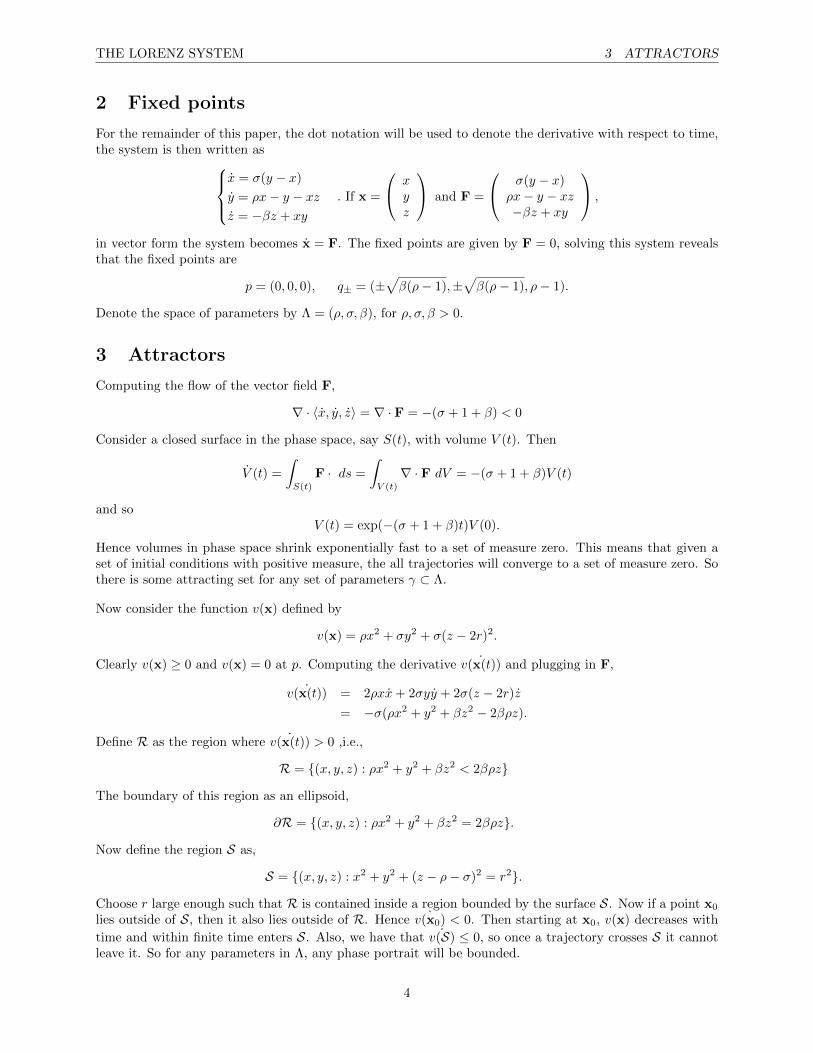
2 Fixed points

For the remainder of this paper, the dot notation will be used to denote the derivative with respect to time,the system is then written as

x = σ(y − x)

y = ρx− y − xzz = −βz + xy

. If x =

xyz

and F =

σ(y − x)ρx− y − xz−βz + xy

,

in vector form the system becomes x = F. The fixed points are given by F = 0, solving this system revealsthat the fixed points are

p = (0, 0, 0), q± = (±√β(ρ− 1),±

√β(ρ− 1), ρ− 1).

Denote the space of parameters by Λ = (ρ, σ, β), for ρ, σ, β > 0.

3 Attractors

Computing the flow of the vector field F,

∇ · 〈x, y, z〉 = ∇ · F = −(σ + 1 + β) < 0

Consider a closed surface in the phase space, say S(t), with volume V (t). Then

V (t) =

∫S(t)

F · ds =

∫V (t)

∇ · F dV = −(σ + 1 + β)V (t)

and soV (t) = exp(−(σ + 1 + β)t)V (0).

Hence volumes in phase space shrink exponentially fast to a set of measure zero. This means that given aset of initial conditions with positive measure, the all trajectories will converge to a set of measure zero. Sothere is some attracting set for any set of parameters γ ⊂ Λ.

Now consider the function v(x) defined by

v(x) = ρx2 + σy2 + σ(z − 2r)2.

Clearly v(x) ≥ 0 and v(x) = 0 at p. Computing the derivative ˙v(x(t)) and plugging in F,

˙v(x(t)) = 2ρxx+ 2σyy + 2σ(z − 2r)z

= −σ(ρx2 + y2 + βz2 − 2βρz).

Define R as the region where ˙v(x(t)) > 0 ,i.e.,

R = (x, y, z) : ρx2 + y2 + βz2 < 2βρz

The boundary of this region as an ellipsoid,

∂R = (x, y, z) : ρx2 + y2 + βz2 = 2βρz.

Now define the region S as,

S = (x, y, z) : x2 + y2 + (z − ρ− σ)2 = r2.

Choose r large enough such that R is contained inside a region bounded by the surface S. Now if a point x0

lies outside of S, then it also lies outside of R. Hence ˙v(x0) < 0. Then starting at x0, v(x) decreases with

time and within finite time enters S. Also, we have that ˙v(S) ≤ 0, so once a trajectory crosses S it cannotleave it. So for any parameters in Λ, any phase portrait will be bounded.

4

THE LORENZ SYSTEM 4 PHASE ANALYSIS

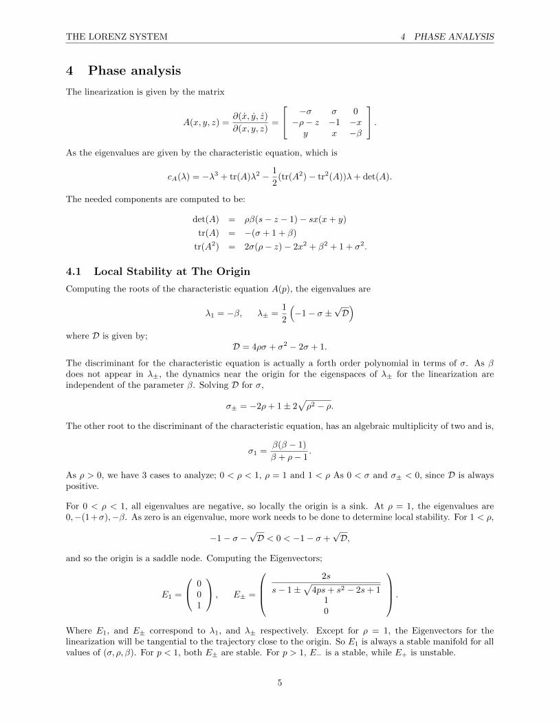
4 Phase analysis

The linearization is given by the matrix

A(x, y, z) =∂(x, y, z)

∂(x, y, z)=

−σ σ 0−ρ− z −1 −xy x −β

.As the eigenvalues are given by the characteristic equation, which is

cA(λ) = −λ3 + tr(A)λ2 − 1

2(tr(A2)− tr2(A))λ+ det(A).

The needed components are computed to be:

det(A) = ρβ(s− z − 1)− sx(x+ y)

tr(A) = −(σ + 1 + β)

tr(A2) = 2σ(ρ− z)− 2x2 + β2 + 1 + σ2.

4.1 Local Stability at The Origin

Computing the roots of the characteristic equation A(p), the eigenvalues are

λ1 = −β, λ± =1

2

(−1− σ ±

√D)

where D is given by;D = 4ρσ + σ2 − 2σ + 1.

The discriminant for the characteristic equation is actually a forth order polynomial in terms of σ. As βdoes not appear in λ±, the dynamics near the origin for the eigenspaces of λ± for the linearization areindependent of the parameter β. Solving D for σ,

σ± = −2ρ+ 1± 2√ρ2 − ρ.

The other root to the discriminant of the characteristic equation, has an algebraic multiplicity of two and is,

σ1 =β(β − 1)

β + ρ− 1.

As ρ > 0, we have 3 cases to analyze; 0 < ρ < 1, ρ = 1 and 1 < ρ As 0 < σ and σ± < 0, since D is alwayspositive.

For 0 < ρ < 1, all eigenvalues are negative, so locally the origin is a sink. At ρ = 1, the eigenvalues are0,−(1+σ),−β. As zero is an eigenvalue, more work needs to be done to determine local stability. For 1 < ρ,

−1− σ −√D < 0 < −1− σ +

√D,

and so the origin is a saddle node. Computing the Eigenvectors;

E1 =

001

, E± =

2s

s− 1±√

4ps+ s2 − 2s+ 110

.

Where E1, and E± correspond to λ1, and λ± respectively. Except for ρ = 1, the Eigenvectors for thelinearization will be tangential to the trajectory close to the origin. So E1 is always a stable manifold for allvalues of (σ, ρ, β). For p < 1, both E± are stable. For p > 1, E− is a stable, while E+ is unstable.

5

THE LORENZ SYSTEM 4 PHASE ANALYSIS

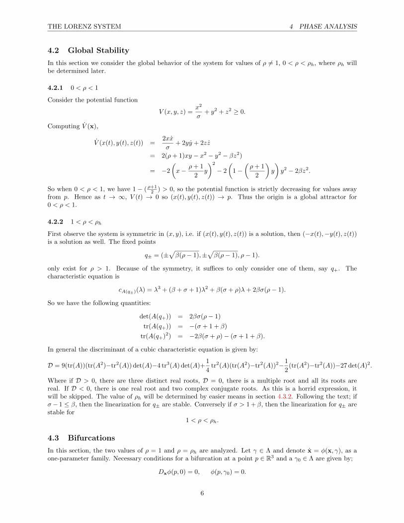
4.2 Global Stability

In this section we consider the global behavior of the system for values of ρ 6= 1, 0 < ρ < ρh, where ρh willbe determined later.

4.2.1 0 < ρ < 1

Consider the potential function

V (x, y, z) =x2

σ+ y2 + z2 ≥ 0.

Computing V (x),

V (x(t), y(t), z(t)) =2xx

σ+ 2yy + 2zz

= 2(ρ+ 1)xy − x2 − y2 − βz2)

= −2

(x− ρ+ 1

2y

)2

− 2

(1−

(ρ+ 1

2

)y

)y2 − 2βz2.

So when 0 < ρ < 1, we have 1 − (ρ+12 ) > 0, so the potential function is strictly decreasing for values away

from p. Hence as t → ∞, V (t) → 0 so (x(t), y(t), z(t)) → p. Thus the origin is a global attractor for0 < ρ < 1.

4.2.2 1 < ρ < ρh

First observe the system is symmetric in (x, y), i.e. if (x(t), y(t), z(t)) is a solution, then (−x(t),−y(t), z(t))is a solution as well. The fixed points

q± = (±√β(ρ− 1),±

√β(ρ− 1), ρ− 1).

only exist for ρ > 1. Because of the symmetry, it suffices to only consider one of them, say q+. Thecharacteristic equation is

cA(q±)(λ) = λ3 + (β + σ + 1)λ2 + β(σ + ρ)λ+ 2βσ(ρ− 1).

So we have the following quantities:

det(A(q+)) = 2βσ(ρ− 1)

tr(A(q+)) = −(σ + 1 + β)

tr(A(q+)2) = −2β(σ + ρ)− (σ + 1 + β).

In general the discriminant of a cubic characteristic equation is given by:

D = 9(tr(A))(tr(A2)−tr2(A)) det(A)−4 tr3(A) det(A)+1

4tr2(A)(tr(A2)−tr2(A))2−1

2(tr(A2)−tr2(A))−27 det(A)2.

Where if D > 0, there are three distinct real roots, D = 0, there is a multiple root and all its roots arereal. If D < 0, there is one real root and two complex conjugate roots. As this is a horrid expression, itwill be skipped. The value of ρh will be determined by easier means in section 4.3.2. Following the text; ifσ− 1 ≤ β, then the linearization for q± are stable. Conversely if σ > 1 + β, then the linearization for q± arestable for

1 < ρ < ρh.

4.3 Bifurcations

In this section, the two values of ρ = 1 and ρ = ρh are analyzed. Let γ ∈ Λ and denote x = φ(x, γ), as aone-parameter family. Necessary conditions for a bifurcation at a point p ∈ R3 and a γ0 ∈ Λ are given by;

Dxφ(p, 0) = 0, φ(p, γ0) = 0.

6

THE LORENZ SYSTEM 4 PHASE ANALYSIS

4.3.1 Supercritical pitchfork bifurcation: ρ = 1

First we have det(A(p)) = βσ(ρ − 1), and so a bifurcation point is at ρ = 1 As ρ < 1 to ρ > 1, thephase portrait gains two fixed points, while the origin goes from stable to unstable. It is easy to see thatDxφ(p, 0) = φ(0, 1) = 0, and local symmetry D2

xφ(p, 0) = 0. This is a pitchfork bifurcation.

In order to determine what type of pitchfork bifurcation this is, we need to extend the system. Introducinga new parameter, r = ρ− 1, we find

y = (r + 1)x− y − xz.The linearization and the eigenvalues remain the same. Previously the eigenvalues are computed to beλi = 0,−(σ + 1),−β. Simplifying the eigenvectors computed above and writing them in a matrix T ;

T =

1 σ 01 −1 00 0 1

.

Where they are ordered by λi = 0,−(σ+ 1),−β, for i = 1, 2, 3. Denote D =diag(λi), a diagonal matrix withthe eigenvalues in the diagonal, i.e. T−1A(p)T = D. Let u = (u, v, w), rewriting the system as F(u) withthe linearization,

F(u) = Du + T−1R(Tu),

where R(x) = F (x)−A(p)x. Computing,

R(Tu) =

0(r − w)(sv − u)(sv + u)(u− v)

, T−1R(Tu)

σ

1 + σ(r − w)(u+ σv)

− 1

1 + σ(r − w)(u+ σv)

(u+ σv)(u− v)

.

Thus the extended system becomes;

u =σ

1 + σ(r − w)(u+ σv)

v = −(1 + σ)v − 1

1 + σ(r − w)(u+ σv)

w = −βw + (u+ σv)(u− v)

r = 0

.

The center manifold will be of the form

W c = (u, v, w, r) : v = h1(u, r), w = h2(u, r), hi(0, 0) = 0, Dhi(0, 0) = 0.

Writing the power series for hi up to quadratic terms,

h1(u, r) = a0 + a0,1u+ a1,0r + a2,0u2 + a1,1ur + a0,2r

2 +O(3)

h2(u, r) = b0 + b0,1u+ b1,0r + b2,0u2 + b1,1ur + b0,2r

2 +O(3)

Applying the conditions hi(0, 0) = 0, Dhi(0, 0) = 0 and truncating the series;

h1(u, r) = a2,0u2 + a1,1ur + a0,2r

2

h2(u, r) = b2,0u2 + b1,1ur + b0,2r

2

Taking derivative with respect to t and using that r = 0;

h1(u, r) = 2a2,0uu+ a1,1ur,

h2(u, r) = 2b2,0uu+ b1,1ur.

Substituting in these values for v and w and matching coefficients reveals,

a2,0 = a1,1 = a0,2 = b1,1 = b0,2 = 0, b2,0 =1

β

7

THE LORENZ SYSTEM 4 PHASE ANALYSIS

What remains is:

u =σ

1 + σ

(ru− u3

β

), r = 0

The equilibrium is stable for r ≤ 0 and unstable for r > 0, which affirms the previous results of ρ ≤ 1and ρ > 1, respectively. The sign in front of the cubic term is negative, which is a supercritical pitchforkbifurcation.

4.3.2 Subcritical Hopf-Bifurcation: ρ = ρh

A Hopf bifurcation occurs when a pair of complex conjugate eigenvalues cross the imaginary axis. Thismeans as ρ < ρh goes to ρ > ρh, the real parts of the eigenvalues vanish at ρ = ρh. The characteristicequation at q± was computed earlier to be;

cA(q±)(λ) = λ3 + (β + σ + 1)λ2 + β(σ + ρ)λ+ 2βσ(ρ− 1)

Plugging in for ρh and solving the eigenvalues are obtained,

λ1 = −(β + σ + 1), λ± = ±ı

√2σ(σ + 1)

σ − β − 1

This is a Hopf bifurcation. The value for ρh can easily be determined considering purely imaginary roots.Let λ = ıµ, for µ ∈ R, plugging this back into the characteristic equation,

cA(q±)(ıµ) = −ıµ3 − (β + σ + 1)µ2 + ıβ(σ + ρ)µ+ 2βσ(ρ− 1) = 0

Taking real and imaginary parts, reveals that

µ2 =2σβ(ρ− 1)

σ + β + 1, µ3 = µβ(σ + ρ)

As µ 6= 0, equating the two expressions and solving for ρ, ρh is found to be

ρh =σ(σ + β + 3)

σ − β − 1

As the eigenvectors are an eye sore, they will be omitted. Instead, notice that if ρ > 1, the characteristicequation cA(q±)(λ) has only positive coefficients. As the origin is unstable. We can conclude, from theelementary symmetric polynomials, that if the roots are real they must be negative. So the points q± arestable for the eigenvalues are real. This affirms what is said in section 4.2.2. Upon some horrible omittedcalculations, for ρh < ρ, the two critical points q± have a two dimensional unstable manifold and a onedimensional stable manifold. At ρ = ρh, there is a two dimensional center manifold. The algebra for thisis a nightmare, but upon doing this, we have that for σ > β + 1 the bifurcation is subcritical. The stablepoints for q± lose their stability by absorbing an unstable periodic orbit. This phenomena is the subject ofthe next section, the origin of these periodic orbits.

4.4 Strange Attracting Sets

A strange attractor is a region in space that is invariant under the evolution of time and attracts mosttrajectories and has a high sensitivity to initial conditions. For 1 < ρ, there is a stable manifold containing pwhich divides integral curves. These curves spiral towards q±. As ρ approaches ρh, the trajectories becomelarger spirals. As ρ > ρh, trajectories on one side of the stable manifold of the origin cross over and startspiraling towards the other side.

8

THE LORENZ SYSTEM 4 PHASE ANALYSIS

4.4.1 Homoclinic Orbits

If a trajectory φ(x, γ∗) starts at a point x0, not on the stable manifold, and reaches x1 in a certain timet1, one would expect that for a small enough perturbation of the initial condition that φ(x, γ∗) starting atx0 ± ε would reach a neighborhood of x1 at the same time t1. As the stable manifold includes the z-axis,perturbing off of it will send a trajectory towards q± depending on the direction of the perturbation. Whatis unexpected is that a small perturbation in the parametric space, φ(x, γ∗± δ), for specific values of γ∗ willcause the trajectory to flow towards another fixed point. For example,

φ(x, (ρ∗, σ, β))→ q+, while φ(x, (ρ∗ + δ, σ, β))→ q−

The change in direction after such a small change in the parameter space can be explained by a homoclinicorbit. Because of the sensitivity to round off error, and the limit of machine precision, these orbits arehard to compute numerically. However, they can be observed numerically with small perturbations in theparametric space. Because of this, one might expect a homoclinic bifurcation to occur. To my knowledgethere is no analytical proof for when homoclinic orbits appear, in general. Proof for specific cases are givenin [2, 3].

4.4.2 Poincare Map

We can deduce the existence of a homoclinic orbit from the the Poincare map. Suppose for a range ofparameters we can construct the following surface. Let S be a surface that contains the fixed points q± andtheir stable manifold such that S intersects the 2D stable manifold at the origin along some curve c(t). Alsochoose S such that any trajectory starting in S returns to S. This defines a Poincare Map, on S\c(t). Nowdenote F = P (S) ∩ S as the return map. First, the curve c(t) is mapped to two point by F , call these c±.By construction, c± are where the unstable manifold of the origin hits S for the first time. Now fixing acoordinate system on S, say (u, v), and let u = 0 define the curve c(t). Write F as,

F (u, v) = (f(u), g(u, v))

Now if the return map F can be filled by a continuum of arcs, such that each arc is taken by the return mapto another arc, then this is a contracting foliation. Assuming this ([4] Ch. 3), 0 < gv(u, v) < 1 for u 6= 0 ag → 0 and u→ 0. We want to observe the behavior of the solution as ρ increase to ρ∗ and beyond, for somevalues ρ∗.

4.4.3 Dynamics at ρ∗

Results from references are summarized. As ρ = ρ∗ the intersection of the unstable manifold of the originwith the return map hits c±, this implies that the unstable manifold of the origin is contained in the stablemanifold, so a homoclinic orbit appears.

For ρ > ρ∗, numerical evidence shows the following. The return map, F has two new fixed points. Thesepoints are from the limit cycles which arise at ρ∗ from the homoclinic orbits. There exists an Cantor-likeinvariant set Ω between these fixed points, this is what some call a strange invariant set. Points that enterΩ stay forever within this region. Furthermore, the dynamics on this set are conjugate to the shift map, s,of two symbols, [4, 6]

s(w) = w2w3w4 . . . , w = w1w2w2 . . . , w ∈ 0, 1.The set of all periodic sequences in Ω is countable and dense in Ω. Suppose that all non-periodic orbitsin Ω can be enumerated as well. Using a cantor diagonal argument, we can construct a sequence with w1

different than in the first sequence, w2 different from the second sequence and so forth. Thus, the set of allnon-periodic orbits must be uncountable. So there exists, within Ω, a countable number of periodic orbitsand an uncountable infinity of aperiodic orbits and orbits that tend to the origin.

On this set Ω, the dynamics also show extreme sensitive dependence on initial data. There are two possibleconclusions that arise from the appearance of this set Ω. First, the two simplest periodic orbits are likely the

9

THE LORENZ SYSTEM 5 NUMERICAL SIMULATIONS AND FIGURES

periodic orbits for which the subcritical Hopf bifurcation at ρh absorbs. Since other periodic orbits cannotbe considered as the z-axis is invariant, an orbit which winds around the axis will never be able to separateitself from it, since it cannot cross it. Second, as the system is always bounded, this invariant set must bethe attractor after the three critical points become unstable.

4.4.4 Asymptotic Behavior

The chaos vanishes for ρ large enough. Let ε = ρ−1/2, and consider the scaling

x = u/ε, y = v/(ε2σ), z = (w/σ + 1)/ε2, t = ετ.

With this scaling the system becomes; u = v − σεuv = −uw − εvw = uv − βε(w + σ)

.

Looking at the leading order terms u = v

v = −uww = uv

.

this lead to a pair of integral curves

u2 − 2v = 2α1, v2 + w2 = α22.

So we have the differential equation that represents and elliptic integral:

w = (2(α2 − w)(w + α2)(w + α1))12

The solution to this equation is always periodic [4].

4.4.5 A Few Remarks

The attracting set has a Cantor-like structure. A strange attractor is one defined as having a non-integerdimension. The Lorenz strange attractor has a Hausdorff dimension which is ∼2.06 [1]. The attractor con-tains a countable infinity of non-stable periodic orbits and an uncountable infinity of aperiodic orbits andtrajectories which terminate at the origin.

An interesting result is that each homoclinic ’explosion’ creates a new strange invariant set, and so therewill be an uncountable number of topologically distinct attractors in any neighborhood of an arbitrary ρ [5].I have found no formulas for finding general ρ∗.

5 Numerical Simulations and Figures

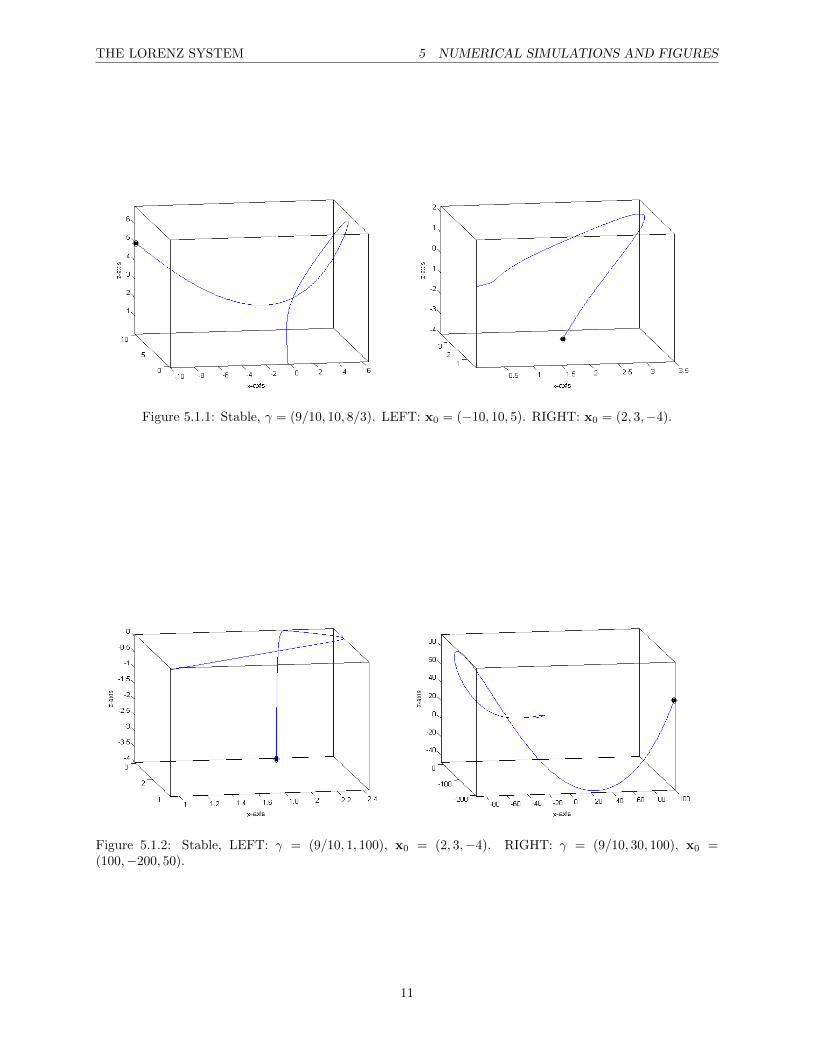
For all figures, the parameter will be denoted by an order triplet γ = (ρ, σ, β). Unless otherwise stated, σ,β, will be fixed at σ = 10, and β = 8/3. The initial condition will be denoted by x0. As the system hasparameters that are of the same order, this is a non-stiff system. For all simulations, MatLab’s ODE45 isused with an error tolerance of 1.e-9. The locations of the initial conditions in all figures is given by a blackdot. The time interval shown for all figures is T = [0, 100], unless otherwise stated.

5.1 Globally stable , 0 < ρ < 1

Several tests show global convergence for various parameters with 0 < ρ < 1, and various initial conditions.

10

THE LORENZ SYSTEM 5 NUMERICAL SIMULATIONS AND FIGURES

Figure 5.1.1: Stable, γ = (9/10, 10, 8/3). LEFT: x0 = (−10, 10, 5). RIGHT: x0 = (2, 3,−4).

Figure 5.1.2: Stable, LEFT: γ = (9/10, 1, 100), x0 = (2, 3,−4). RIGHT: γ = (9/10, 30, 100), x0 =(100,−200, 50).

11

THE LORENZ SYSTEM 5 NUMERICAL SIMULATIONS AND FIGURES

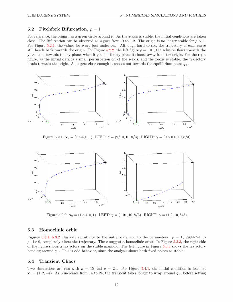
5.2 Pitchfork Bifurcation, ρ = 1

For reference, the origin has a green circle around it. As the z-axis is stable, the initial conditions are takenclose. The Bifurcation can be observed as ρ goes from .9 to 1.2. The origin is no longer stable for ρ > 1.For Figure 5.2.1, the values for ρ are just under one. Although hard to see, the trajectory of each curvestill bends back towards the origin. For Figure 5.2.2, the left figure ρ = 1.01, the solution flows towards they-axis and towards the xy-plane; when it gets on the xy-plane it shoots away from the origin. For the rightfigure, as the initial data is a small perturbation off of the z-axis, and the z-axis is stable, the trajectoryheads towards the origin. As it gets close enough it shoots out towards the equilibrium point q+.

Figure 5.2.1: x0 = (1.e-4, 0, 1). LEFT: γ = (9/10, 10, 8/3). RIGHT: γ = (99/100, 10, 8/3)

Figure 5.2.2: x0 = (1.e-4, 0, 1). LEFT: γ = (1.01, 10, 8/3). RIGHT: γ = (1.2, 10, 8/3)

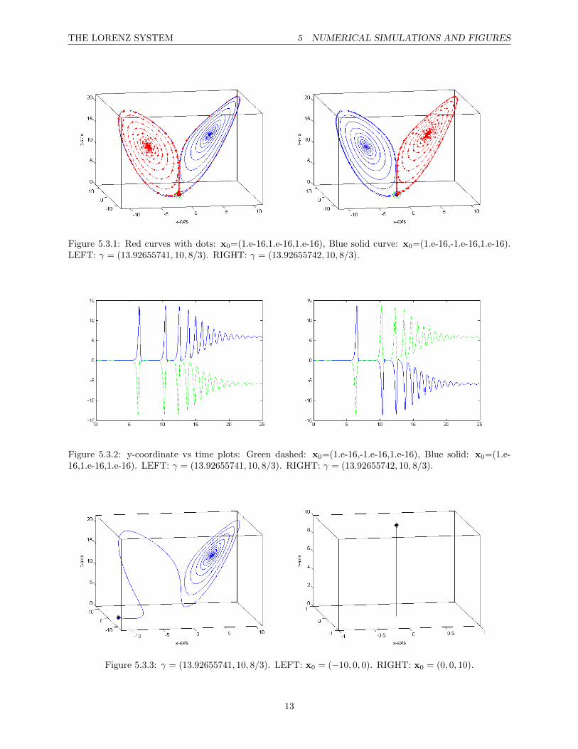
5.3 Homoclinic orbit

Figures 5.3.1, 5.3.2 illustrate sensitivity to the initial data and to the parameters. ρ = 13.92655741 toρ+1.e-9, completely alters the trajectory. These suggest a homoclinic orbit. In Figure 5.3.3, the right sideof the figure shows a trajectory on the stable manifold, The left figure in Figure 5.3.3 shows the trajectorybending around q−. This is odd behavior, since the analysis shows both fixed points as stable.

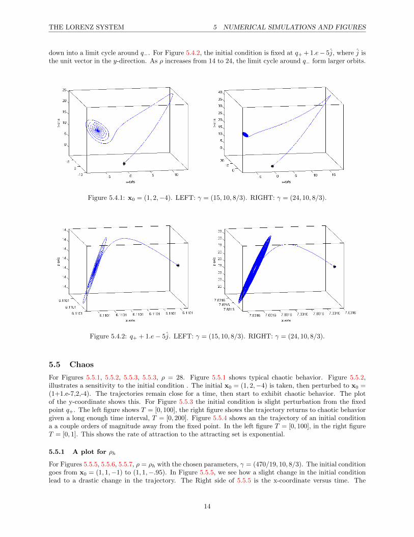
5.4 Transient Chaos

Two simulations are run with ρ = 15 and ρ = 24. For Figure 5.4.1, the initial condition is fixed atx0 = (1, 2,−4). As ρ increases from 14 to 24, the transient takes longer to wrap around q+, before setting

12

THE LORENZ SYSTEM 5 NUMERICAL SIMULATIONS AND FIGURES

Figure 5.3.1: Red curves with dots: x0=(1.e-16,1.e-16,1.e-16), Blue solid curve: x0=(1.e-16,-1.e-16,1.e-16).LEFT: γ = (13.92655741, 10, 8/3). RIGHT: γ = (13.92655742, 10, 8/3).

Figure 5.3.2: y-coordinate vs time plots: Green dashed: x0=(1.e-16,-1.e-16,1.e-16), Blue solid: x0=(1.e-16,1.e-16,1.e-16). LEFT: γ = (13.92655741, 10, 8/3). RIGHT: γ = (13.92655742, 10, 8/3).

Figure 5.3.3: γ = (13.92655741, 10, 8/3). LEFT: x0 = (−10, 0, 0). RIGHT: x0 = (0, 0, 10).

13

THE LORENZ SYSTEM 5 NUMERICAL SIMULATIONS AND FIGURES

down into a limit cycle around q−. For Figure 5.4.2, the initial condition is fixed at q+ + 1.e− 5j, where j isthe unit vector in the y-direction. As ρ increases from 14 to 24, the limit cycle around q− form larger orbits.

Figure 5.4.1: x0 = (1, 2,−4). LEFT: γ = (15, 10, 8/3). RIGHT: γ = (24, 10, 8/3).

Figure 5.4.2: q+ + 1.e− 5j. LEFT: γ = (15, 10, 8/3). RIGHT: γ = (24, 10, 8/3).

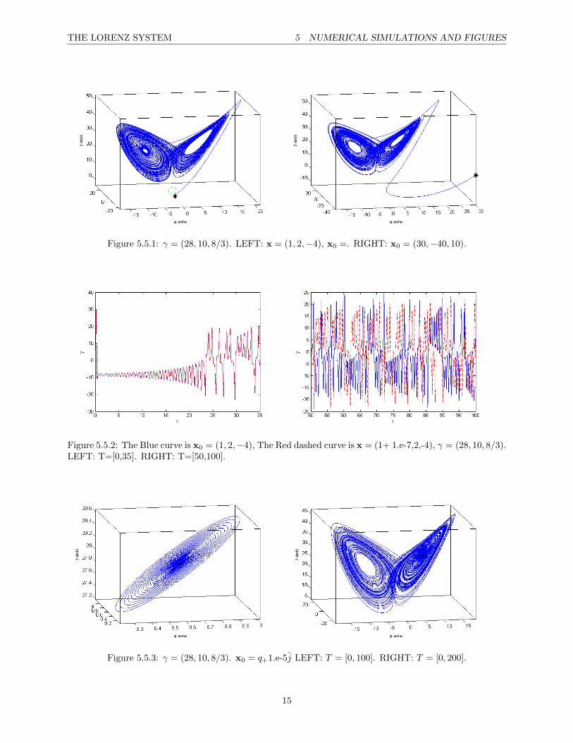
5.5 Chaos

For Figures 5.5.1, 5.5.2, 5.5.3, 5.5.3, ρ = 28. Figure 5.5.1 shows typical chaotic behavior. Figure 5.5.2,illustrates a sensitivity to the initial condition . The initial x0 = (1, 2,−4) is taken, then perturbed to x0 =(1+1.e-7,2,-4). The trajectories remain close for a time, then start to exhibit chaotic behavior. The plotof the y-coordinate shows this. For Figure 5.5.3 the initial condition is slight perturbation from the fixedpoint q+. The left figure shows T = [0, 100], the right figure shows the trajectory returns to chaotic behaviorgiven a long enough time interval, T = [0, 200]. Figure 5.5.4 shows an the trajectory of an initial conditiona a couple orders of magnitude away from the fixed point. In the left figure T = [0, 100], in the right figureT = [0, 1]. This shows the rate of attraction to the attracting set is exponential.

5.5.1 A plot for ρh

For Figures 5.5.5, 5.5.6, 5.5.7, ρ = ρh with the chosen parameters, γ = (470/19, 10, 8/3). The initial conditiongoes from x0 = (1, 1,−1) to (1, 1,−.95). In Figure 5.5.5, we see how a slight change in the initial conditionlead to a drastic change in the trajectory. The Right side of 5.5.5 is the x-coordinate versus time. The

14

THE LORENZ SYSTEM 5 NUMERICAL SIMULATIONS AND FIGURES

Figure 5.5.1: γ = (28, 10, 8/3). LEFT: x = (1, 2,−4), x0 =. RIGHT: x0 = (30,−40, 10).

Figure 5.5.2: The Blue curve is x0 = (1, 2,−4), The Red dashed curve is x = (1+ 1.e-7,2,-4), γ = (28, 10, 8/3).LEFT: T=[0,35]. RIGHT: T=[50,100].

Figure 5.5.3: γ = (28, 10, 8/3). x0 = q+1.e-5j LEFT: T = [0, 100]. RIGHT: T = [0, 200].

15

THE LORENZ SYSTEM 5 NUMERICAL SIMULATIONS AND FIGURES

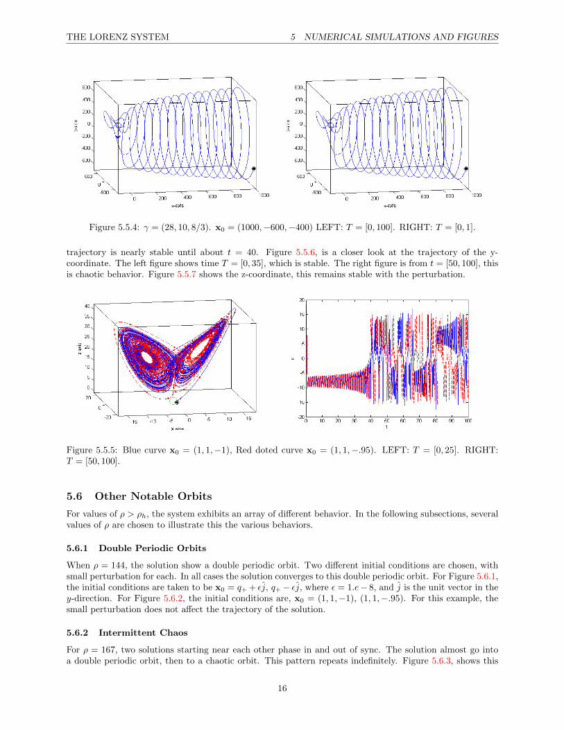
Figure 5.5.4: γ = (28, 10, 8/3). x0 = (1000,−600,−400) LEFT: T = [0, 100]. RIGHT: T = [0, 1].

trajectory is nearly stable until about t = 40. Figure 5.5.6, is a closer look at the trajectory of the y-coordinate. The left figure shows time T = [0, 35], which is stable. The right figure is from t = [50, 100], thisis chaotic behavior. Figure 5.5.7 shows the z-coordinate, this remains stable with the perturbation.

Figure 5.5.5: Blue curve x0 = (1, 1,−1), Red doted curve x0 = (1, 1,−.95). LEFT: T = [0, 25]. RIGHT:T = [50, 100].

5.6 Other Notable Orbits

For values of ρ > ρh, the system exhibits an array of different behavior. In the following subsections, severalvalues of ρ are chosen to illustrate this the various behaviors.

5.6.1 Double Periodic Orbits

When ρ = 144, the solution show a double periodic orbit. Two different initial conditions are chosen, withsmall perturbation for each. In all cases the solution converges to this double periodic orbit. For Figure 5.6.1,the initial conditions are taken to be x0 = q+ + εj, q+− εj, where ε = 1.e− 8, and j is the unit vector in they-direction. For Figure 5.6.2, the initial conditions are, x0 = (1, 1,−1), (1, 1,−.95). For this example, thesmall perturbation does not affect the trajectory of the solution.

5.6.2 Intermittent Chaos

For ρ = 167, two solutions starting near each other phase in and out of sync. The solution almost go intoa double periodic orbit, then to a chaotic orbit. This pattern repeats indefinitely. Figure 5.6.3, shows this

16

THE LORENZ SYSTEM 5 NUMERICAL SIMULATIONS AND FIGURES

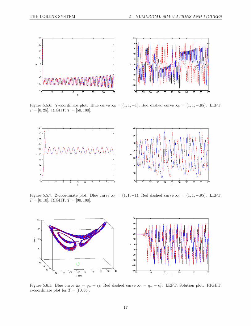
Figure 5.5.6: Y-coordinate plot: Blue curve x0 = (1, 1,−1), Red dashed curve x0 = (1, 1,−.95). LEFT:T = [0, 25]. RIGHT: T = [50, 100].

Figure 5.5.7: Z-coordinate plot: Blue curve x0 = (1, 1,−1), Red dashed curve x0 = (1, 1,−.95). LEFT:T = [0, 10]. RIGHT: T = [90, 100].

Figure 5.6.1: Blue curve x0 = q+ + εj, Red dashed curve x0 = q+ − εj. LEFT: Solution plot. RIGHT:x-coordinate plot for T = [10, 35].

17

THE LORENZ SYSTEM 6 MATLAB CODE

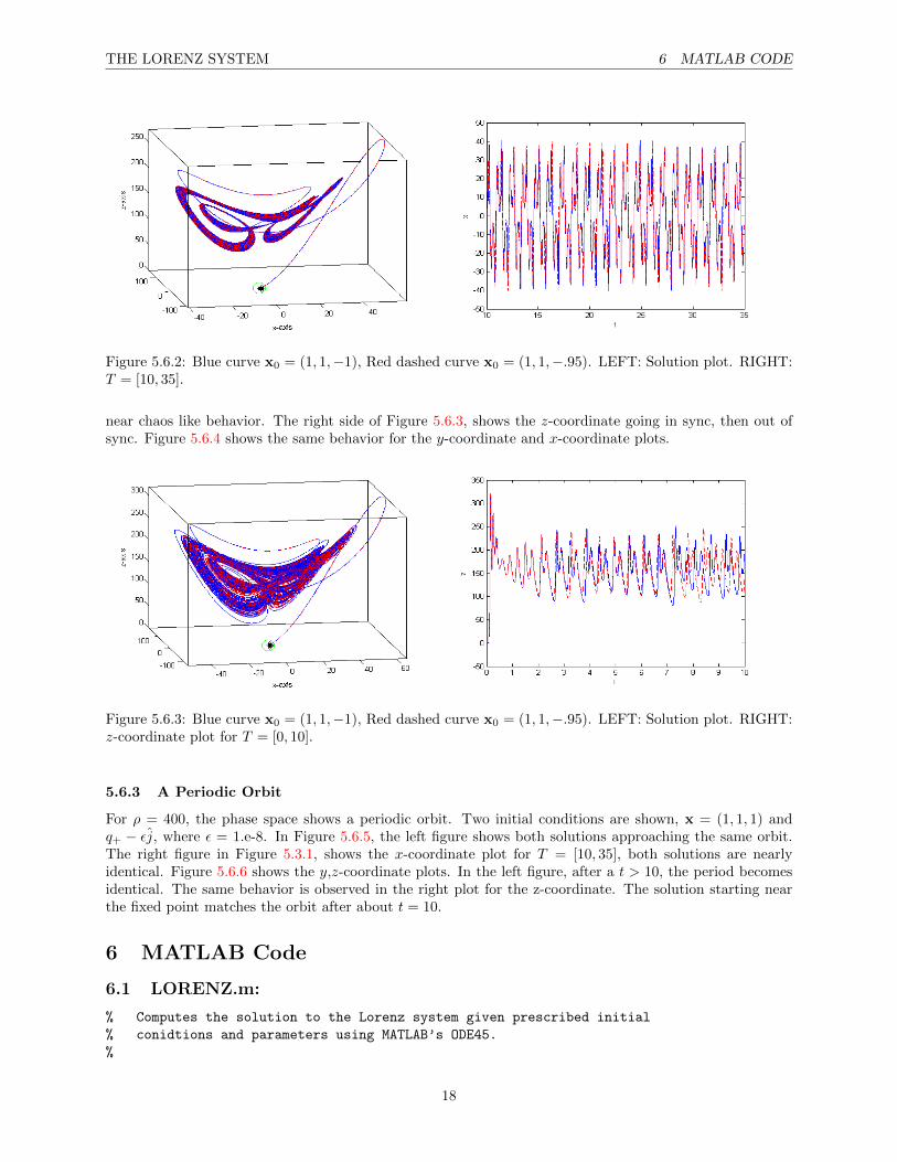
Figure 5.6.2: Blue curve x0 = (1, 1,−1), Red dashed curve x0 = (1, 1,−.95). LEFT: Solution plot. RIGHT:T = [10, 35].

near chaos like behavior. The right side of Figure 5.6.3, shows the z-coordinate going in sync, then out ofsync. Figure 5.6.4 shows the same behavior for the y-coordinate and x-coordinate plots.

Figure 5.6.3: Blue curve x0 = (1, 1,−1), Red dashed curve x0 = (1, 1,−.95). LEFT: Solution plot. RIGHT:z-coordinate plot for T = [0, 10].

5.6.3 A Periodic Orbit

For ρ = 400, the phase space shows a periodic orbit. Two initial conditions are shown, x = (1, 1, 1) andq+ − εj, where ε = 1.e-8. In Figure 5.6.5, the left figure shows both solutions approaching the same orbit.The right figure in Figure 5.3.1, shows the x-coordinate plot for T = [10, 35], both solutions are nearlyidentical. Figure 5.6.6 shows the y,z-coordinate plots. In the left figure, after a t > 10, the period becomesidentical. The same behavior is observed in the right plot for the z-coordinate. The solution starting nearthe fixed point matches the orbit after about t = 10.

6 MATLAB Code

6.1 LORENZ.m:

% Computes the solution to the Lorenz system given prescribed initial

% conidtions and parameters using MATLAB’s ODE45.

%

18

THE LORENZ SYSTEM 6 MATLAB CODE

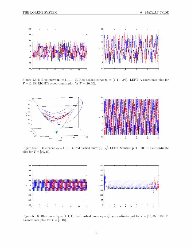
Figure 5.6.4: Blue curve x0 = (1, 1,−1), Red dashed curve x0 = (1, 1,−.95). LEFT: y-coordinate plot forT = [0, 35] RIGHT: x-coordinate plot for T = [10, 35].

Figure 5.6.5: Blue curve x0 = (1, 1, 1), Red dashed curve q+−εj. LEFT: Solution plot. RIGHT: x-coordinateplot for T = [10, 35].

Figure 5.6.6: Blue curve x0 = (1, 1, 1), Red dashed curve q+− εj. y-coordinate plot for T = [10, 35] RIGHT:z-coordinate plot for T = [0, 10].

19

THE LORENZ SYSTEM 6 MATLAB CODE

% INPUT:

% RHO - Scaled Rayleigh number.

% SIGMA - Prandtl number.

% BETA - Geometry ascpet ratio.

% INI - Initial point.

% T - Time interval T = [ta,tb]

% EPS - ode45 solver precision

%

% OUTPUT:

% x - x-coodinate of solution.

% y - y-coodinate of solution.

% z - z-coodinate of solution.

% t - Time inteval for [x(t),y(t),z(t)]

%

Initializations

if nargin<4

eps = 1.e-9;

T = [0 100];

ini = [1 1 1];

end

if nargin < 5

T = [0 100];

ini = [1 1 1];

end

if nargin < 6

ini = [1 1 1];

end

options = odeset(’RelTol’,eps,’AbsTol’,[eps eps eps/10]);

Solve system

[t,X] = ode45(@(T,X) sys(X, sigma, rho, beta), T, ini, options);

Set output

x = X(:,1); y = X(:,2); z = X(:,3);

6.2 LORENZ SYS.M

function dx = lorenz_sys(X, sigma, rho, beta)

% Computes the vector field for the Lorenz system:

% x’ = sigma*(y-x)

% y’ = x*(rho - z) - y

% z’ = x*y - beta*z

% INPUT:

% RHO - Scaled Rayleigh number.

% SIGMA - Prandtl number.

% BETA - Geometry ascpet ratio.

% OUTPUT:

% dx - Vector field for Lorenz system.

20

THE LORENZ SYSTEM 6 MATLAB CODE

System

dx = zeros(3,1);

dx(1) = sigma*(X(2) - X(1));

dx(2) = X(1)*(rho - X(3)) - X(2);

dx(3) = X(1)*X(2) - beta*X(3);

6.3 LORENZ SYS VEC.M

function dx = lorenz_sys_vec(x,y,z, sigma, rho, beta)

% Computes the vector field for the Lorenz system for vector input.

% x’ = sigma*(y-x)

% y’ = x*(rho - z) - y

% z’ = x*y - beta*z

% INPUT:

% RHO - Scaled Rayleigh number.

% SIGMA - Prandtl number.

% BETA - Geometry ascpet ratio.

% OUTPUT:

% dx - Vector field for Lorenz system.

System

dx = zeros(3,length(x));

dx(1,:) = sigma*(y - x);

dx(2,:) = x.*(rho - z) - y;

dx(3,:) = x.*y - beta*z;

6.4 PLOTTING SCRIPT.M

Set parameters

close all; clear all; clc;

% Test parameters for rho with sigma = 10, beta = 8/3;

% rho < 1; %Stable Trajectories

% rho = 1; %Pitchfork Bifurcation near origin

% rho = 13.92655741; %Homoclinic orbit near origin

% rho = 13.92655742; %Homoclinic orbit near origin

% rho = 28; %Chaos

% rho = sigma*(sigma + beta + 3)/(sigma-beta-1);%Hopf bifurcation

%

%Use rho, for solution with a single initial condtions.

%Use rho1,rho2 to compare two initial conditions

%rho1 = 40;

%rho2 = rho1;

rho = 100;

sigma = 10;

beta = 8/3;

Various initial conditions

%p = [1.e-16,1.e-16,1.e-16]; $Pertubation of origin

%p = [1.e-16,-1.e-16,1.e-16]; $Pertubation of origin

%p = [sqrt(beta*(rho - 1)),sqrt(beta*(rho - 1)),rho - 1];% fixed point

21

THE LORENZ SYSTEM 6 MATLAB CODE

%p = [sqrt(beta*(rho - 1))-1.e-8,sqrt(beta*(rho - 1)),rho - 1];

% Pertubation of fixed point

%

%p1 = [1,1,-1];

%p2 = [1,1,-.95];

p = [1,1,1];

Set Solver options and plot options

T = [0 100]; %Time interval for solution T = [ta,tb];

eps = 1.e-9; %Persicion for ode45

plot_data = 0; %0 = Single initial condition

%1 = Two phase portaits together

%2 = Two phase portaits seperately

if plot_data == 0

[X,Y,Z,t] = lorenz(rho, sigma, beta, p, T, eps);

else

[X1,Y1,Z1,t1] = lorenz(rho1, sigma, beta, p1, T, eps);

[X2,Y2,Z2,t2] = lorenz(rho2, sigma, beta, p2, T, eps);

end

Plot

if plot_data == 1

M = floor(sqrt(length(t1))/2);

figure

plot3(X1,Y1,Z1,’--r’);

hold on

plot3(X1(1:M:end),Y1(1:M:end),Z1(1:M:end),’r’,’Marker’,’.’,’linestyle’, ’none’);

plot3(p1(1),p1(2),p1(3),’MarkerSize’,20,’Marker’,’.’,’color’, ’k’);

plot3(p1(1),p1(2),p1(3),’MarkerSize’,10,’Marker’,’d’,’color’, ’k’);

plot3(0,0,0,’MarkerSize’,15,’Marker’,’o’,’color’, ’g’);

axis tight;

box on

xlabel(’x-axis’);

zlabel(’z-axis’);

view([-10 15])

xlab = get(gca,’xlabel’);

set(xlab,’rotation’,3)

%

figure

plot3(X2,Y2,Z2);

hold on

plot3(p2(1),p2(2),p2(3),’MarkerSize’,20,’Marker’,’.’,’color’, ’k’);

plot3(p2(1),p2(2),p2(3),’MarkerSize’,10,’Marker’,’d’,’color’, ’k’);

plot3(0,0,0,’MarkerSize’,15,’Marker’,’o’,’color’, ’g’);

axis tight;

box on

xlabel(’x-axis’);

zlabel(’z-axis’);

view([-10 15])

xlab = get(gca,’xlabel’);

set(xlab,’rotation’,3)

elseif plot_data == 2

22

THE LORENZ SYSTEM 6 MATLAB CODE

figure

plot3(X1,Y1,Z1);

hold on

plot3(X2,Y2,Z2,’--r’);

plot3(p1(1),p1(2),p1(3),’MarkerSize’,20,’Marker’,’.’,’color’, ’k’);

plot3(p1(1),p1(2),p1(3),’MarkerSize’,10,’Marker’,’d’,’color’, ’k’);

plot3(p2(1),p2(2),p2(3),’MarkerSize’,20,’Marker’,’.’,’color’, ’k’);

plot3(p2(1),p2(2),p2(3),’MarkerSize’,10,’Marker’,’d’,’color’, ’k’);

plot3(0,0,0,’MarkerSize’,15,’Marker’,’o’,’color’, ’g’);

axis tight;

box on

xlabel(’x-axis’);

zlabel(’z-axis’);

view([-10 15])

xlab = get(gca,’xlabel’);

set(xlab,’rotation’,3)

else

M = floor(sqrt(length(t))/2);

figure

plot3(X,Y,Z);

hold on

plot3(p(1),p(2),p(3),’MarkerSize’,20,’Marker’,’.’,’color’, ’k’);

plot3(p(1),p(2),p(3),’MarkerSize’,10,’Marker’,’d’,’color’, ’k’);

plot3(0,0,0,’MarkerSize’,15,’Marker’,’o’,’color’, ’g’);

axis tight;

box on

xlabel(’x-axis’);

zlabel(’z-axis’);

view([-10 15])

xlab = get(gca,’xlabel’);

set(xlab,’rotation’,3)

end

if plot_data == 1 || plot_data == 2

X Plots

figure

plot(t1,X1);

hold on

plot(t2,X2,’--r’);

hold off

xlabel(’t’)

ylabel(’x’)

%

figure

K1 = find(t1 >50);

plot(t1(K1),X1(K1));

hold on

K2 = find(t2 >50);

plot(t2(K2),X2(K2),’--r’);

hold off

xlabel(’t’)

ylabel(’x’)

%

23

THE LORENZ SYSTEM 6 MATLAB CODE

figure

L1 = find(t1 < 35);

plot(t1(L1),X1(L1));

hold on

L2 = find(t2 < 35);

plot(t2(L2),X2(L2),’--r’);

hold off

xlabel(’t’)

ylabel(’x’)

Y plots

figure

K1 = find(t1 >50);

plot(t1(K1),Y1(K1));

hold on

K2 = find(t2 >50);

plot(t2(K2),Y2(K2),’--r’);

hold off

xlabel(’t’)

ylabel(’y’)

%

figure

L1 = find(t1 < 35);

plot(t1(L1),Y1(L1));

hold on

L2 = find(t2 < 35);

plot(t2(L2),Y2(L2),’--r’);

hold off

xlabel(’t’)

ylabel(’y’)

Z-plots

figure

K1 = find(t1 >90);

plot(t1(K1),Z1(K1));

hold on

K2 = find(t2 >90);

plot(t2(K2),Z2(K2),’--r’);

hold off

xlabel(’t’)

ylabel(’z’)

%

figure

L1 = find(t1 < 10);

plot(t1(L1),Z1(L1));

hold on

L2 = find(t2 < 10);

plot(t2(L2),Z2(L2),’--r’);

hold off

xlabel(’t’)

ylabel(’z’)

end

24

THE LORENZ SYSTEM BIBLIOGRAPHY

Bibliography

[1] P. Grassberger and I. Procaccia. Measuring the strangeness of strange attractors. Physica D: NonlinearPhenomena, 9(12):189 – 208, 1983.

[2] B. Hassard and J. Zhang. Existence of a homoclinic orbit of the lorenz system by precise shooting. SIAMJournal on Mathematical Analysis, 25(1):179–196, 1994.

[3] S. Hastings and W. Troy. A proof that the lorenz equations have a homoclinic orbit. Journal of DifferentialEquations, 113(1):166 – 188, 1994.

[4] C. Sparrow. The Lorenz Equations: Bifurcations, Chaos, and Strange Attractors. Applied MathematicalSciences. Springer New York, 1982.

[5] R. Williams. The structure of lorenz attractors. Publications Mathmatiques de l’Institut des Hautes tudesScientifiques, 50(1):73–99, 1979.

[6] J. Yorke and E. Yorke. Metastable chaos: The transition to sustained chaotic behavior in the lorenzmodel. Journal of Statistical Physics, 21(3):263–277, 1979.

25