The Impact of the French Securities Transaction Tax on ... · The Impact of the French Securities...

1

The Impact of the French Securities Transaction Tax on Market Liquidity and Volatility ◊◊◊◊

Gunther CAPELLE-BLANCARD ∗∗∗∗

Olena HAVRYLCHYK ϒϒϒϒ

First draft: April 2013 Current draft: December 2013

Abstract: In this paper, we assess the impact of the securities transaction tax (STT) introduced in France in 2012 on market liquidity and volatility. To identify causality, we rely on the unique design of this tax that is imposed only on large French firms, all listed on Euronext. This provides two reliable control groups (smaller French firms and foreign firms also listed on Euronext) and allows using difference-in-difference methodology to isolate the impact of the tax from other economic changes occurring simultaneously. We find that the STT has reduced trading volume, but we find no effect on theoretically based measures of liquidity, such as price impact, and no significant effect on volatility. The results are robust if we rely on different control groups (German stocks), analyze dynamic effects or construct a control group by propensity score matching.

Keywords: Financial transaction tax, Securities transaction tax, Tobin tax, Volatility, Liquidity, Euronext.

JEL Classification: G21, H25.

L'impact de la taxation des transactions financières sur la liquidité et la volatilité des actions françaises

Résumé : Dans cet article, nous évaluons l’impact de la taxe sur les transactions financières (TTF), introduite en France en 2012, sur la liquidité et la volatilité des actions. Cette taxe se prête particulièrement bien à une étude d’impact dans la mesure où seules les grandes entreprises qui ont leur siège social en France sont taxées, permettant ainsi d’identifier deux groupes de contrôle : les autres entreprises françaises et les entreprises étrangères, toutes cotées sur Euronext. Nous utilisons la méthode des doubles-différences pour isoler l’impact de la taxe d’autres changements économiques survenus simultanément. Il en ressort que la TTF a réduit les volumes de transaction, mais sans que cela n’ait d’effet sur la liquidité. Nous ne décelons, en outre, aucun effet sur la volatilité. Ces résultats sont robustes même en utilisant d’autres groupes de contrôle (les actions allemandes) ou en appliquant une méthode d’appariement sur les scores de propension.

Mots-clés : Taxe sur les transactions financières, Taxe Tobin, Volatilité, Liquidité, Euronext.

◊ The authors thank Michael Brennan, Masahisa Fujita, Kaku Furuya, Atsushi Nakajima, Valérie Mignon, Masayuki Morikawa, Andy Mullineux, Urszula Szczerbowicz, Wing Wah Tham, Taisuke Uchino and Laurent Weill, as well as participants of the RIETI and Daito Bunka University seminars, the GDR Money, Banking and Finance conference (June 2013), the AHRC FinCris workshop (‘Taxing Banks Fairly’, Sept. 2013), and the IFMA conference on Finance and Banking (Dec. 2013) for helpful comments. O. Havrylchyk is grateful for an excellent working environment at the RIETI where she stayed as a Visiting scholar during September 2013. This paper previously circulated under the title “Securities Transaction Tax and Market Behavior: Evidence from Euronext”. Preliminary results have been published in “La Lettre du Cepii” No. 331 (March 2013). ∗ Université Paris 1 Panthéon-Sorbonne & Paris School of Economics. E-mail: [email protected]. Corresponding author: 106-112 Bd. de l’Hôpital 75013 Paris, France. Phone: +33 (0)1 44 07 82 60. ϒ Université Paris Ouest Nanterre La Défense & Cepii. E-mail: [email protected].

2

“And then there’s the proposal for a Financial Transactions Tax... Even to be considering this at a time when we are struggling to get our

economies growing is quite simply madness”.

David Cameron, British Prime Minister

“And then there’s the idea of taxing financial transactions, which have exploded in recent decades. The economic value of all this trading is

dubious at best. In fact, there’s considerable evidence suggesting that too much trading is going on… it suggests that to the extent that taxing

financial transactions reduces the volume of wheeling and dealing, that would be a good thing.”

Paul Krugman, economist and Nobel Laureate

1. Introduction: A ‘madness’ or a ‘good thing’?

Will a tax on financial transactions curb speculative activity and render financial markets

more stable? Or will it hurt market liquidity and price discovery, thus, making markets even

more volatile? Although the idea to tax financial transactions dates to Keynes (1936) and

Tobin (1978), it has received a renewed attention of policy leaders as a result of the global

financial crisis. The idea appears to be particularly popular in Europe. In June 2011, the

European Commission proposed to set up a financial transaction tax (FTT) as a source of the

EU budget, but there was no unanimous support within the EU member states for a common

FTT. Hence, in September 2012 eleven EU states chose to introduce a FTT, which was

initially planned to come in force in 2014.1 This will be the first time that the FTT is

introduced in a group of countries, but different versions of FTT exist in almost thirty

countries in the world, including the United Kingdom, Switzerland, Hong-Kong, China, and

Brazil. In some countries stocks and derivatives are taxed, like in the EU project, but most of

the financial transaction taxes are levied only on stocks – and are referred as to securities

transaction taxes (STT).

The debate on FTT is among the most visible and newsworthy aspects of financial regulation

and one of the most controversial topics.2 According to a survey conducted by the European

1 Gabor (2013) provides an in-depth analysis of the political economics of the European Commission’s proposal. 2 To give a broad idea, the entry “Tobin tax” is listed in the top 250 controversial issues among Wikipedia editors for the category “Politics/Economics”, along with such entries as Capital punishment, Holocaust, Gun

3

Commission, FTT is supported by six out ten Europeans. The strength of the support varies

considerably among the countries: in France, Germany or Italy seven out of ten respondents

are in favor of the FTT, while there are only four in Sweden or the UK and only three in the

Netherlands.3 At the same time, European political leaders are strongly divided on the merits

of FTT and the opposition is expressed in harsh terms. For the Swedish Finance Minister,

Anders Borg, such tax is “very dangerous”, its Dutch counterpart, Jan Kees de Jager fears

“devastating results”, UK Prime Minister, David Cameron considers FTT as a “madness”.4

Several leading economists have also expressed strong views on this topic. For some

(including Kenneth Rogoff5), FTT is not only inefficient, but counterproductive, while for

others (among which Paul Krugman6, Avinash Persaud7, Jeffrey Sachs8), it might be a win-

win initiative.

Despite the popularity of FTT and the surrounding controversies, the academic literature is

rather scarce.9 Theoretically, FTT should decrease trading volume due to an increase in

transaction costs, but the ultimate impact on volatility depends on what type of traders is

driven from the market. In the framework of the Efficient Market Hypothesis, agents are

supposed to be perfectly rational and stock prices reflect fundamentals. Increasing liquidity

and speculation are stabilising factors. Accordingly, the increase in transaction costs due to

the FTT will reduce liquidity by driving away rational agents, thus, automatically amplifying

market volatility (Schwert and Seguin, 1993; Dooley, 1996; Kupiec, 1996; Subrahmanyam,

1998; Amihud and Mendelson, 2003). Alternatively, if noise traders (either uniformed or not

perfectly rational) prevent stock prices from converging to their fundamental value, increasing

trading is destabilising. By discouraging noise traders’ activity, the FTT will dampen market

volatility (Stiglitz, 1989; Summers and Summers, 1989; Eichengreen, Tobin and Wyplosz,

1995).

Bloomfield, O’Hara and Saar (2009) provide an elegant framework which encompassed the

two previous paradigms. They use a laboratory market to investigate the behavior of noise

traders and their impact on the market. While FTT do “reduce volume, [it] do[es] not affect

politics, Same-sex marriage, etc. If we restrict the list to economic issues, it appears in the top 10 together with some broad matters like Capitalism or Communism. 3 EU 27 (In favor: 61%; Opposed: 25%), France (71%; 19%), Germany (74%; 16%), Italy (72%; 14%), Sweden (45%; 46%), UK (43%; 41%), Netherlands (36%; 53%). Source: Standard Eurobarometer n°74, January 2011. 4 Quotes are from The New York Times, Oct. 9, 2012 and The Telegraph, Jan. 26, 2012. 5 Kenneth Rogoff, The wrong tax for Europe, Project Syndicate, Oct. 3, 2011. 6 Paul Krugman, Things to tax, The New York Times, Nov. 27, 2011. 7 Avinash Persaud, EU’s financial transaction tax is feasible, and if set right, desirable, VoxEu, Sept. 30, 2011. 8 Jeffrey Sachs, Obama, the G20, and the 99 Percent, Huffington Post, Nov. 1, 2011. 9 A comprehensive literature survey is provided in Matheson (2011) or McCulloch and Pacillo (2011).

4

spreads and price impact measures, and have at most a weak effect on the informational

efficiency of prices.” They explained this result by arguing that the FTT has driven away both

rational and noise traders. Song and Zhang (2005) come to a similar conclusion in a general

equilibrium setting.

Hau (1998) also develops a model in which endogenous entry of traders may increase the

capacity of the market to absorb exogenous supply risk, but at the same time it adds noise and

endogenous trading risk. The competitive entry equilibrium is characterized by excessive

market entry and excessively volatile prices. A positive tax on entrants can decrease trader

participation and volatility while increasing market efficiency. Finally, there might be a U-

shaped relationship between liquidity and excessive volatility (Haberer, 2004; Ehrenstein et

al., 2005). At low levels of market volume, greater liquidity reduces excess volatility.

However, after a certain point, the confusion caused by speculation creates a positive

relationship between liquidity and excess volatility.

Since theoretical predictions are ambiguous, it is important to examine the impact of the FTT

empirically. In this paper, we study the introduction, in 2012, of a 0.2 percent tax on daily

acquisitions of French equity securities. We are interested in calculating the impact of this

STT on market quality measured by market liquidity and volatility. Our contribution to the

existing literature is twofold. First, we believe that our study provides a rigorous investigation

of causality between STT and market quality. This is possible due to the unique design of the

French STT. As the tax is levied only on large French firms – all of them listed on Euronext –

this provides two control groups: smaller French firms and foreign firms also listed on

Euronext. Hence, we can rely on difference-in-difference methodology to isolate the impact

of the tax from other economic or regulatory developments during the analyzed period.

Although some earlier studies follow this approach, their control groups are not fully

convincing because stocks are traded in a completely different institutional environment, such

as foreign or over-the-counter market (Umlauf, 1993; Pomeranets and Weaver, 2012). It is

important to note that the French STT is virtually the only tax in the world that has affected

differently large and small firms.10

Our second contribution consists in a rigorous analysis of different dimensions of market

liquidity and volatility. Usual measures of liquidity in the academic literature can be classified

in three main categories: volume-based measures (volume and turnover ratio), transaction cost

10 In March 2013, Italy has introduced a similar STT which does not apply to companies whose average market capitalization is lower than €500 million.

5

measures (bid-ask spread), and price-impact measures (liquidity ratio and price reversal).

These measures gauge different aspects of market liquidity and are often complements and

not substitutes (Vayanos and Wang, 2012). Similarly, we plan to investigate the impact on

market volatility measured by several alternative measures, such as absolute and squared

close-to-close returns, daily conditional variance, and price range.

Our study shows that the introduction of the French STT has reduced market volume, but

there is no effect on theoretically based measure of liquidity, such as price impact. As to

volatility measures, the results are statistically insignificant. The results are robust if we rely

on different control groups (German stocks included in DAX and MDAX), analyze dynamic

effects or construct a control group by propensity score matching. Overall, our results give

support to the laboratory observations made by Bloomfield, O’Hara and Saar (2009). For

policy purposes, we can conclude that the French STT cannot be used as a Pigouvian tax to

decrease market volatility, but it does not lead to harmful distortions either.

Recently, several unpublished studies have independently examined the impact of the French

STT (Becchetti, Ferrari and Trenta, 2013; Colliard and Hoffman, 2013; Haferkorn and

Zimmermann, 2013; Meyer, Wagener, and Weinhardt, 2013). All these studies rely on a

difference-in-difference methodology, but they only examined short-term effects (over a

maximum period of a few months after the introduction of the tax). They are mainly

interested in the impact on liquidity, and do not provide much evidence on volatility. Overall,

they support our results.

The remainder of the paper is structured as follows. Section 2 provides an overview of the

empirical literature. Section 3 describes the data, the empirical strategy and the construction

of the liquidity and volatility measures. Section 4 reports our empirical results. Section 5

provides several robustness tests: different samples (smaller but more homogeneous), and

different method (propensity score matching). Section 6 concludes.

2. Overview of the empirical literature

Since theoretical predictions are ambiguous, a number of papers empirically examine the

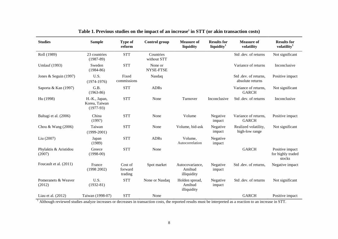
impact of the STT on financial market11 (see Table 1 for a summary).12 When measuring the

impact on liquidity (often proxied by volume), studies arrive at similar results as four out of 11 Empirical evidence form the housing market in Singapore is recently provided by Fu, Qian and Yeung (2013). 12 A parallel body of literature examines the impact of the tick size on stock market quality. See Hau (2006) for a panel data study on the French market.

6

five studies in Table 1 find negative impact on liquidity and one study finds statistically

insignificant result. As to volatility, results are inconclusive. Six out of eleven studies find

inconclusive or statistically insignificant results; four studies find an increase in volatility for

some subsamples, and one study finds a decrease in volatility. However, most of these studies

suffer from methodological shortcomings because they do not address endogeneity problems.

One potential source of endogeneity relates to reverse causality. Since transaction taxes are

often perceived as a tool to reduce market volatility, it is likely that they are introduced in

countries and during periods exhibiting high market volatility. Another source of endogeneity

is due to simultaneity and omitted variable biases. In other words, we do not know how the

same market would have behaved if the tax had not been introduced, as these studies do not

allow us to isolate the impact of the STT from other economic developments or regulatory

changes during the same time period. The three studies that suggest an increase of the stock

market volatility (Baltagi, Li and Li, 2006; Phylaktis and Aristidou, 2007; Liau, 2012) do not

control for simultaneity and omitted variable biases and, therefore, should be considered with

caution.

Several studies attempt to overcome the above endogeneity problems by relying on

difference-in-difference methodologies. In order to isolate the effect of the tax from other

effects that could influence volatility, these studies compare the differential impact of STT

changes on treatment and control groups. Different types of control groups have been

considered: American Depository Receipts, foreign stocks, over-the-counter and forward

markets.

Umlauf (1993) studies the introduction of the 1% securities transaction tax in Sweden in 1984

and its increase to 2% in 1986. To analyze the impact on volatility, he relies on the control

group that consists of the New York Stock Exchange and London Stock Exchange indexes.

Umlauf (1993) mentions that the Swedish tax was introduced for political reasons and, hence,

the reaction of Swedish stock market could reflect increased political uncertainty that goes

beyond the introduction of the tax. In this context, a control group from a different country

does not allow isolating the effect of the tax from other economic and political developments

in Sweden.

Saporta and Kan (1997) analyze changes in the UK stamp duty during 1955-1996 by

comparing shares of UK listed companies that are subject to the tax with the corresponding

American Depository Receipts (ADRs). Although such approach is attractive, it only allows

analyzing the impact on market volumes, because stocks and ADRs prices are closely related

7

due to arbitrage. Moreover, the reliability of their results suffers from small size of their

control group that consists of only four ADRs. Liu (2007) relies on a similar methodology to

analyze STT change in 1989 in Japan. His control group consists of 22 Japanese ADRs and he

finds a negative impact on volumes.

Pomeranets and Weaver (2012) analyze nine changes in the New York state STT between

1932 and 1981 that affected stocks traded on the New York Stock Exchange. They find that

the STT has a negative impact on traded volumes, but no statistically significant impact on

market volatility. Moreover, they find no consistent evidence that traders avoid the tax by

changing their location of trades. Unfortunately, these results are difficult to generalize

because the STT in New York was abolished in 1981 and since then, the increase in traded

volume has been tremendous. In terms of methodology, for tax changes from 1975, they

compare stocks traded on the New York Stock Exchange (treatment group) to stocks traded

on the Nasdaq (control group). This approach was used earlier by Jones and Seguin (1997)

who studied the 1975 introduction of lower, negotiated commissions on U.S. national stock

exchanges that are analogous to a STT. The choice of such control group suffers from the fact

that the decision to be listed or not on the organized exchange is likely to be endogenous,

because reporting and regulatory requirements are smaller for stocks that are only traded on

the Nasdaq. Moreover, the difference-in-difference analysis is performed only for volatility,

but not for liquidity.

Lastly, Foucault, Sraer and Thesmar (2011) analyze a reform of the French stock market that

suppresses the possibility to trade with end-of-month settlement (the “Règlement Mensuel”,

similar to a forward market) for highly liquid stocks and, thus, raises the relative cost of

speculative trading for retail investors, who are often regarded as noise traders. This reform

could be compared to the introduction of a STT. The authors rely on difference-in-difference

methodology (with spot market as a control group) and show that the reform has significantly

reduced the volatility of stocks.

8

Table 1. Previous studies on the impact of an increase1 in STT (or akin transaction costs)

Studies Sample Type of reform

Control group Measure of liquidity

Results for liquidity 1

Measure of volatility

Results for volatility 1

Roll (1989) 23 countries (1987-89)

STT Countries without STT

Std .dev. of returns Not significant

Umlauf (1993) Sweden (1984-86)

STT None or NYSE-FTSE

Variance of returns Inconclusive

Jones & Seguin (1997) U.S. (1974-1976)

Fixed commissions

Nasdaq Std .dev. of returns, absolute returns

Positive impact

Saporta & Kan (1997) G.B. (1963-86)

STT ADRs Variance of returns, GARCH

Not significant

Hu (1998) H.-K., Japan, Korea, Taiwan

(1977-93)

STT None Turnover Inconclusive Std .dev. of returns Inconclusive

Baltagi et al. (2006) China (1997)

STT None Volume Negative impact

Variance of returns, GARCH

Positive impact

Chou & Wang (2006) Taiwan (1999-2001)

STT None Volume, bid-ask Negative impact

Realized volatility, high-low range

Not significant

Liu (2007) Japan (1989)

STT ADRs Volume, Autocorrelation

Negative impact

Phylaktis & Aristidou (2007)

Greece (1998-00)

STT None GARCH Positive impact for highly traded

stocks Foucault et al. (2011) France

(1998 2002) Cost of forward trading

Spot market Autocovariance, Amihud

illiquidity

Negative impact

Std .dev. of returns,

Negative impact

Pomeranets & Weaver (2012)

U.S. (1932-81)

STT None or Nasdaq Holden spread, Amihud

illiquidity

Negative impact

Std .dev. of returns Not significant

Liau et al. (2012) Taiwan (1998-07) STT None GARCH Positive impact 1 Although reviewed studies analyze increases or decreases in transaction costs, the reported results must be interpreted as a reaction to an increase in STT.

9

3. Data and methodology

3.1. The French securities transaction tax

In January 2012, the French President Nicolas Sarkozy announced the introduction a 0.1

percent tax on financial transactions related to French stocks.13 The terms of the tax have been

detailed in the Article 5 of the Supplementary Budget Act for 2012 (Act No. 2012-354 of 14

March 2012), published in the Official Gazette (Journal Officiel) on 15 March 2012 and

completed with the fiscal instruction 3°P-3-12 (BOI n°61 of 3 August 2012).14 The tax has

three components: i) a tax on acquisitions of French equity securities and similar instruments

(Article 235 ter ZD); ii) a tax on orders cancelled in the context of high frequency trading

(Article 235 ter ZD bis); iii) a tax on naked sovereign credit default swaps (Article 235 ter ZD

ter). After the election of François Hollande and shortly before its introduction, the rate of the

tax on acquisitions of equity securities was doubled to 0.2 percent. The tax came into force on

August 1, 2012.

According to the initial estimate of the government, the tax should have yielded €1.6 billion in

2013, that is around 0.2% of total fiscal revenues. One year later, based on the first result for

2012, the estimate was adjusted downwards by fifty percent. In fact, the total revenue for

2012 (August-December) was equal to €0.2 billion: 99.5% from acquisitions of equity

securities and 0.5% from transactions on naked sovereign CDS. The tax on high-frequency

trading generated no revenue (Finance committee of the French parliament’s lower house,

Information report n°1328 of 25 July 2013), as will be discussed later.

Hence, the main component of the taxing scheme is the tax on acquisitions of equity securities

and similar instruments, defined as shares and other securities that provide or could provide

access to capital or voting rights (hereafter, the STT). The tax does not apply to units in

collective investment schemes and financial contracts (including options, futures and

warrants). Exemptions also include: i) issuance of equity securities on the primary market, ii)

transactions by a clearing house or a central depository, iii) activities related to market making

(either for providing liquidity on a regular and continuous basis, or in response to orders

initiated by clients, or by hedging positions arising from the fulfilment of the previous tasks),

13 It should be noted that a STT already existed in France: it was called “Impôt sur les opérations de bourse”, created in 1893 and abrogated in 2007 (see Figure A in appendix). 14 Detailed of the French FTT are available on the website of the French Ministry of Economy: https://www.tresor.economie.gouv.fr/File/376507.

10

iv) acquisitions in the context of liquidity agreements, v) intra-group and restructuring

transactions, vi) temporary transfers of securities, vii) employee saving scheme transactions,

viii) exchange or conversion of bonds into shares. To prevent tax avoidance, the tax is due

regardless of the place of establishment of the regulated market on which the security is

traded, regardless of the place of establishment or residence of the parties to the transaction,

and regardless of the place where the contract was entered into.

Importantly for our identification strategy, the STT must be paid on the acquisition of stocks

issued by companies whose headquarters are located in France and with market values of

more than 1 billion Euros on January 1st of the year of taxation. The list of the stocks subject

to this tax was published on 2th of July 2012 and it is composed of 109 stocks listed on

Euronext. Hence, the design of the tax allows the split of the sample into a treatment and a

control group with an ad-hoc cutoff of €1 billion.

Among the 109 stocks subject to the French STT, 59 are included in the Euronext 100 index

and 30 – in the Next 150. The remaining 20 stocks are not included in those indexes because

their free float is too low (e.g. CIC or Autoroute Paris-Rhin-Rhone, with a free float lower

than 3%) or because the company is controlled by a block of shareholders (e.g. Areva is held

at 83% by the Commissariat à l’Energie Atomique and the French Government, Euler Hermes

is held at 67% by the founding family and at 18% by LVMH) – see Table A in appendix.

Finally, the STT is collected once a day and, hence, intraday trading is not affected. To tax

high-frequency trading, an additional tax of 0.01 percent was introduced on the amount of

cancelled or modified orders, in excess of a threshold of 80%, within a time-span of half a

second (Article 235 ter ZD bis and decree n°2012-957, August 6, 2012). As it was mentioned

earlier, this tax on high-frequency trading had generated zero revenue in 2012. According to

the French financial markets regulator (Autorité des Marchés Financiers), the market share of

high-frequency trading in 2012 has remained virtually stable (slightly declined from 20% to

18%) and so, there is strong evidence that the tax on high-frequency trading has been

bypassed.15 In this context, this study focuses on daily measures of market quality.

15 Subsequently, in October 2013, the Finance committee of the French parliament’s lower house proposed to extent the STT to intraday trading. However, the French government was not in favor of this amendment which was finally rejected.

11

3.2. The sample

Our initial sample consists of all the stocks included in the Euronext 100 or the Next 150

indexes. Our period extends over 12 months: 6 months before the introduction of the STT

(February 2012-July 2012) and 6 months after the introduction of the STT (August 2012-

January 2013).16 Data are daily. Thus, our panel is composed of a maximum of 254 days *

250 firms = 63,500 observations. All the data are extracted from Datastream. For each stock,

we have the opening and closing (adjusted) prices, the volume, the number of shares, the bid-

ask spread quoted at the close of the market, the highest and the lowest prices achieved on the

day.

We exclude from the initial sample six companies that have experienced a takeover bid in

2012, plus a company for which information on trading volume is missing. This leaves 61,722

observations, i.e. 97% of the initial sample. Firms subject to the French STT represent about

one third of the sample. Further, for robustness checks, we exclude companies for which stock

price was lower than €2 at least one day over the period or the total volume over the period

below k€60,000. This robustness sample contains 82% of the initial one – see Table B in

appendix.

3.3. A difference-in-difference approach

To identify the impact of the STT, we rely on the generalized version of the difference-in-

difference (DiD) methodology, and, hence we estimate the following econometric model:

�� = �� + �� + �� + �� + ��, (1)

where �� is a measure of market liquidity or volatility for the firm i at time t, � is a firm

dummy variable, � is a time dummy variable, � �� is a dummy variable that is equal to 1

for large French firms (market values of more than €1 billion) after the introduction of the

STT on 1 August 2012 and �� is an error term. Our coefficient of interest is ��. We estimate

the equation allowing firm-level clustering of the errors that is allowing for correlation of the

error term over time within firms (Bertrand et al., 2004).

The design of the French STT is well suited for DiD methodology because French authorities

have introduced a tax on only large French firms traded on Euronext and, hence, providing us

16 We considered also a period of 1 year before the introduction of the STT to test the robustness. Results are available on request.

12

with two valid control groups: small French firms and foreign firms traded on Euronext. Time

dummy variables capture all other changes in regulatory and economic environment during

the period that should have affected large and small banks in a similar manner. Firm dummy

variables capture differences between firms that are constant over time. In this way, the DiD

methodology allows for differences in market behavior between large and small firms before

the introduction of the STT, but its underlying assumption is that these differences would

remain constant if the STT had not been introduced (the “parallel trends” assumption).

We estimate equation (1) for three different subsamples based on two treatment groups and

three control groups. In the first subsample, we consider all the firms that are included in the

Euronext 100 index. All the French firms (59 firms, Panel A) in this subsample are subject to

the tax, and our control group consists of foreign firms that are not subject to the STT (40

firms, Panel B17). These foreign firms have headquarters in Belgium (11), Great Britain (1),

Luxembourg (2), Netherlands (21), Portugal (4) or Spain (1). Second, we consider all French

firms included in the Next 150 (78 firms). In this case, our treatment group is composed of

large midcap French firms with a market value above 1 billion and that are subject to the STT

(29 firms, Panel C18), while our control group consists of small mid-cap French firms with

market value of less than 1 billion and that are not subject to the STT (49 firms, Panel D).

Finally, we consider firms included in the Next 150 with the exception of small midcap

French firms. Hence, our treatment group is, as before, the large French midcaps (29 firms,

Panel C) and our control group consists of foreign firms included in Next 150 (66 firms, Panel

E19).

The main advantage of our study is that stocks included both in the treatment and the control

groups are traded on the same stock exchange and, hence, with the same organizational,

regulatory and competitive environment, and hence are usually subject to the same shocks.

Nevertheless, both control groups used in this study (the foreign firms and the small midcaps)

have their advantages and disadvantages. The advantage of the smaller French stocks is that

they allow a better control for country-specific shocks, because they belong to the same

country as treatment group. The advantage of foreign firms traded on Euronext is that their

size is more comparable with the treatment group. One can question, however, whether this

17 TNT Express, which experienced a takeover bid in 2012, has been removed from the initial sample. 18 CFAO, which experienced a takeover bid in 2012, has been removed from the initial sample. 19 Degven, Dockwise, Mediq, and LBI International which experienced a takeover bid in 2012, have been removed from the initial sample. Espirito Santo Finl GP has been also removed due to infrequent trading.

13

control group allows isolating the effect of the STT from other shocks that could have

affected France during the same time period.

One may argue that the STT might have a global impact on all Euronext stocks due to co-

movement in liquidity. Cespa and Foucault (2011) have shown that liquidity spillover can be

positive or negative depending on the cost of price information. In either case, our estimate of

the impact could be biased if we consider securities from Euronext as a control group.

Therefore, we use also a control group consisting of German stocks traded on Deutsche

Boerse (Xetra) and included in the DAX 30 or the MDAX 50 indexes. This sample is less

likely to be impacted by potential co-movement in liquidity.

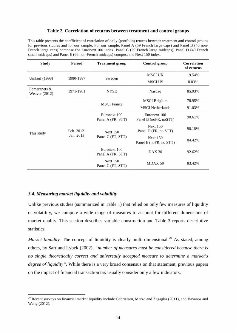
The choice of the control groups is intended to be theoretically grounded. To confirm their

relevance, we report in Table 2 the correlation of daily portfolio returns between treatment

and control groups and compare it with previous studies that relied on control groups

(Umlauf, 1993; Pomeranets & Weaver, 2012). Because we do not have access to data samples

of earlier papers, we consider, as a proxy, the main stock indexes in Sweden, the US and the

UK. To insure comparability, we first do the same for French, Belgium, Dutch and German

stocks. Then we measure the correlation for our exact samples.

Looking at our sample, we find that the correlation of returns between the French, the

Belgium and the Dutch stock indexes is high. Precisely, for the largest firms (Euronext 100)

correlation of daily returns between Panel A (FR, STT) and Panel B (noFR, no STT) is more

than 90% over the period. The correlation for mid-caps (Next 150) is slightly lower, but still

large: 90% between Panel C (FR, STT) and Panel D (FR, no STT) and 84% between Panel C

and Panel E (noFRR, noSTT). Finally, co-movement with firms listed on Deutsche Boerse is

also high with a correlation of 92% between our Panel A and the DAX index and a correlation

of 83% between Panel C and the MDAX index.

Our correlation results compare well to earlier studies. Umlauf (1993) analyzed the impact of

the STT on the Swedish market, relying on the US and UK markets as control groups. The

correlations of 9-19% are very low due to the large distance (geographical, economical,

institutional…) of Sweden to the UK or the US in the 1980s, therefore making these stock

markets not very suitable as control groups. Pomeranets & Weaver (2012) consider the impact

of a STT on the NYSE by relying on Nasdaq as a control group. Although stocks listed on the

NYSE and the Nasdaq are very different, the correlation of returns (85%) seems sufficiently

large to allow confidence in such control group.

14

Table 2. Correlation of returns between treatment and control groups

This table presents the coefficient of correlation of daily (portfolio) returns between treatment and control groups for previous studies and for our sample. For our sample, Panel A (59 French large caps) and Panel B (40 non-French large caps) compose the Euronext 100 index. Panel C (29 French large midcaps), Panel D (49 French small midcaps) and Panel E (66 non-French midcaps) compose the Next 150 index.

Study Period Treatment group Control group Correlation of returns

Umlauf (1993) 1980-1987 Sweden MSCI UK 19.54%

MSCI US 8.83%

Pomeranets & Weaver (2012)

1971-1981 NYSE Nasdaq 85.93%

This study Feb. 2012- Jan. 2013

MSCI France MSCI Belgium 78.95%

MSCI Netherlands 91.03%

Euronext 100 Panel A (FR, STT)

Euronext 100 Panel B (noFR, noSTT)

90.61%

Next 150 Panel C (FT, STT)

Next 150 Panel D (FR, no STT)

90.15%

Next 150 Panel E (noFR, no STT)

84.42%

Euronext 100 Panel A (FR, STT)

DAX 30 92.62%

Next 150 Panel C (FT, STT)

MDAX 50 83.42%

3.4. Measuring market liquidity and volatility

Unlike previous studies (summarized in Table 1) that relied on only few measures of liquidity

or volatility, we compute a wide range of measures to account for different dimensions of

market quality. This section describes variable construction and Table 3 reports descriptive

statistics.

Market liquidity. The concept of liquidity is clearly multi-dimensional.20 As stated, among

others, by Sarr and Lybek (2002), “number of measures must be considered because there is

no single theoretically correct and universally accepted measure to determine a market’s

degree of liquidity”. While there is a very broad consensus on that statement, previous papers

on the impact of financial transaction tax usually consider only a few indicators.

20 Recent surveys on financial market liquidity include Gabrielsen, Marzo and Zagaglia (2011), and Vayanos and Wang (2012).

15

Usual measures of liquidity in the academic literature can be classified – from the less to the

most sophisticated – in three main categories: volume-based measures, transaction cost

measures (bid-ask spread), and price-impact measures (liquidity ratio). Accordingly, in this

study, we use the following variables:

• Volume, Vi,t= Number of shares traded for the stock i on day t *Pi,t where Pi,t is the

closing price for the stock i on the day t; number of shares is expressed in thousands.

• Bid-ask spread, Si,t = 2*100*(PAi,t–PBi,t) / (PAi,t+PBi,t) where PAi,t and PBi,t are the

asking price and the bid price offered for the stock i at close of market on day t,

respectively; bid-ask spread is expressed in percentage.

• Liquidity Ratio, LRi,t = Vi,t / | Ri,t

| where Ri,t is the continuously compounded returns,

log(Pi,t / Pi,t–1), for the stock i on the day t, respectively; liquidity ratio is expressed in

thousands euros of trade for a price change of one percent.

These measures gauge different aspects of market liquidity and can be considered as

complements and not substitutes. Measuring liquidity by trading volume is the most intuitive

way because it captures markets’ breadth and depth. However, this measure suffers from

some drawbacks (Vayanos and Wang, 2012). First, trading activity does not provide a direct

estimate of the costs of trading. Second, trading activity can be influenced by other variables

than market imperfections, such as the supply of an asset, the number of investors holding it

and the size of their trading needs. Another widely used measure of liquidity is bid-ask spread

and it is used to assess tightness. Note that this measure provides no information on the prices

at which larger transactions take place. By the same token, it provides no information on how

the market might respond to a long sequence of transactions in the same direction. Market’s

response to large buying or selling pressure is an important aspect of illiquidity.

Liquidity denotes the ability to trade large quantities quickly, at low cost, and without moving

the price. Several indicators of market resiliency address this definition and we choose to use

the liquidity ratio, which assesses how much traded volume is necessary to induce a price

change of one percent21: higher ratio is associated with higher liquidity.

For the sake of robustness, we also consider the turnover and price reversal:

21 There are several alternative to compute this ratio, which idea goes back to Dolley (1938) and Beach (1939). This ratio can be also expressed as the inverse of the illiquidity measure of Amihud (2002). Common alternatives is to consider the difference between the highest and the lowest daily prices instead of the return, and to adjust traded volume for market capitalization. However, empirical results are not qualitatively different and, consequently, are not reported.

16

• Turnover, Ti,t = 100*Number of shares traded for the stock i on day t / total number of

shares for the stock i on day t available to ordinary investors; turnover is expressed in

percentage.

• Price Reversal, PRi,t is minus the coefficient of a regression of Ri,t on Vi,t–1*sign(Ri,t–1),

controlling for Ri,t–1.

Similar to volume, turnover captures markets’ breadth and depth, but takes into account the

number of shares available for sale. Price reversal is a measure of price impact, like the

liquidity ratio, albeit less intuitive. It is based on the idea that, if markets are illiquid, trades

should generate transitory deviations between price and fundamental value22: higher price

reversal is associated with lower liquidity.

Market volatility. Similarly, there are several alternative measures to assess market volatility.

According to Engle and Gallo (2006), for instance, “ the concept of volatility itself is

somewhat elusive, as many ways exist to measure it and hence to model it”. In this paper, we

consider three different metrics:

• Squared Return, SRi,t = (Ri,t)² where Ri,t= log(Pi,t / Pi,t–1).

• Conditional variance, CVi,t is proxied by a GARCH(1,1) model – the model for the

conditional mean is an AR(1) with a constant.23

• High-low range, HLRi,t = (log PHi,t – log PLi,t)² / 4 log(2) where PHi,t and PLi,t are the

highest price and the lowest price achieved for the stock i on the day t, respectively.

Squared close-to-close return is a common estimator of the daily variance.24 Volatility

clustering has been extensively documented, so we estimate daily conditional variance,

proxied by a conventional GARCH(1,1) model over a period of 12 months (February 2012 –

January 2013).25 Finally, we use a measure of price range, defined as the scaled difference

between the highest and the lowest prices achieved on a day. The range provides volatility

information from the entire intraday price path, without the need of high frequency data. 22 The idea dates back to Niederhoffer and Osborne (1966), but was popularized by Roll (1984) who uses the autocovariance of daily stock returns to proxy price reversal. Campbell, Grossman, and Wang (1993) show that the autocovariance of returns correlates negatively with trading volume and, then, suggest to use a conditional estimator. Since then, several specifications have been proposed; amongst them, the measure of Pastor Stambaugh (2003), which our indicator is inspired by, is one of the most used. 23 We have considered alternative GARCH models, but it does not change the results. 24 Jones and Seguin (1997) and Pomeranets and Weaver (2012) consider an unbiased estimator of the standard deviation computed as √(π/2)| Ri,t

|. Because the first term is a constant, it does not influence the econometric results later on. 25 We consider two specifications of the mean equation: a first one with only a constant term and an AR(1). This choice does not have any consequence, and we report only results corresponding to the AR(1).

17

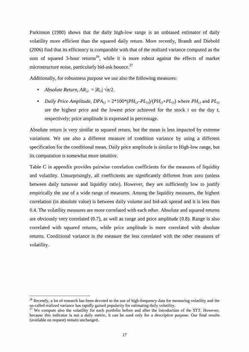
Parkinson (1980) shows that the daily high-low range is an unbiased estimator of daily

volatility more efficient than the squared daily return. More recently, Brandt and Diebold

(2006) find that its efficiency is comparable with that of the realized variance computed as the

sum of squared 3-hour returns26, while it is more robust against the effects of market

microstructure noise, particularly bid-ask bounce.27

Additionally, for robustness purpose we use also the following measures:

• Absolute Return, ARi,t = |Ri,t| √π/2.

• Daily Price Amplitude, DPAi,t = 2*100*(PHi,t–PLi,t)/(PHi,t+PLi,t) where PHi,t and PLi,t

are the highest price and the lowest price achieved for the stock i on the day t,

respectively; price amplitude is expressed in percentage.

Absolute return is very similar to squared return, but the mean is less impacted by extreme

variations. We use also a different measure of condition variance by using a different

specification for the conditional mean. Daily price amplitude is similar to High-low range, but

its computation is somewhat more intuitive.

Table C in appendix provides pairwise correlation coefficients for the measures of liquidity

and volatility. Unsurprisingly, all coefficients are significantly different from zero (unless

between daily turnover and liquidity ratio). However, they are sufficiently low to justify

empirically the use of a wide range of measures. Among the liquidity measures, the highest

correlation (in absolute value) is between daily volume and bid-ask spread and it is less than

0.4. The volatility measures are more correlated with each other. Absolute and squared returns

are obviously very correlated (0.7), as well as range and price amplitude (0.8). Range is also

correlated with squared returns, while price amplitude is more correlated with absolute

returns. Conditional variance is the measure the less correlated with the other measures of

volatility.

26 Recently, a lot of research has been devoted to the use of high-frequency data for measuring volatility and the so-called realized variance has rapidly gained popularity for estimating daily volatility. 27 We compute also the volatility for each portfolio before and after the introduction of the STT. However, because this indicator is not a daily metric, it can be used only for a descriptive purpose. Our final results (available on request) remain unchanged.

18

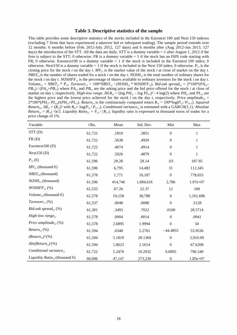
Table 3. Descriptive statistics of the sample

This table provides some descriptive statistics of the stocks included in the Euronext 100 and Next 150 indexes (excluding 7 firms that have experienced a takeover bid or infrequent trading). The sample period extends over 12 months: 6 months before (Feb. 2012-July. 2012, 127 days) and 6 months after (Aug. 2012-Jan. 2013, 127 days) the introduction of the STT. All the data are daily. STT is a dummy variable = 1 after August 1, 2012 if the firm is subject to the STT; 0 otherwise. FR is a dummy variable = 1 if the stock has an ISIN code starting with FR; 0 otherwise. Euronext100 is a dummy variable = 1 if the stock is included in the Euronext 100 index; 0 otherwise. Next150 is a dummy variable = 1 if the stock is included in the Next 150 index; 0 otherwise. Pi,t is the closing price for the stock i on the day t. MVi,t is the market value of the stock i at close of market on the day t. NBSTi,t is the number of shares traded for a stock i on the day t. NOSHi,t is the total number of ordinary shares for the stock i on day t. NOSHFFi,t is the percentage of shares available to ordinary investors for the stock i on day t. Volumei,t = NBSTi,t * Pi,t. Turnoveri,t = 100*NBSTi,t / (NOSHi,t * NOSHFFi,t). Bid-ask spreadi,t = 2*100*(PAi,t–PBi,t) / (PAi,t+PBi,t) where PAi,t and PBi,t are the asking price and the bid price offered for the stock i at close of market on day t, respectively. High-low range, HLRi,t = (log PHi,t – log PLi,t)² / 4 log(2) where PHi,t and PLi,t are the highest price and the lowest price achieved for the stock i on the day t, respectively. Price amplitudei,t = 2*100*(PHi,t–PLi,t)/(PHi,t+PLi,t). Returni,t is the continuously computed return Ri,t = 100*log(Pi,t / Pi,t–1). Squared Returni,t, SRi,t = (Ri,t)² with Ri,t= log(Pi,t / Pi,t–1). Conditional variancei,t is estimated with a GARCH(1,1). Absolute Returni,t = |Ri,t| √π/2. Liquidity Ratioi,t = Vi,t / |

Ri,t |; liquidity ratio is expressed in thousand euros of trades for a

price change of 1%.

Variable Obs. Mean Std. Dev. Min Max

STT (D) 61,722 .1810 .3851 0 1

FR (D) 61,722 .5638 .4959 0 1

Euronext100 (D) 61,722 .4074 .4914 0 1

Next150 (D) 61,722 .5926 .4879 0 1

Pi,t (€) 61,596 29.28 28.14 .03 187.95

MVi,t (thousand €) 61,596 6,795 14,482 31 112,345

NBSTi,t (thousand) 61,578 1,771 10,187 0 778,655

NOSHi,t (thousand) 61,596 414,746 1,084,616 2,786 1.97e+07

NOSHFFi,t (%) 61,555 67.26 22.37 12 100

Volumei,t (thousand €) 61,578 19,158 38,788 0 1,161,686

Turnoveri,t (%) 61,537 .0048 .0088 0 .5128

Bid-ask spreadi,t (%) 61,301 .3493 .7022 .0100 28.5714

High-low rangei,t 61,578 .0004 .0014 0 .0941

Price amplitudei,t (%) 61,578 2.6895 1.9994 0 50

Returni,t (%) 61,594 .0348 2.2761 –44.4855 53.9536

(Returni,t)² (%) 61,594 5.1819 28.1369 0 2,910.99

Abs(Returni,t) (%) 61,594 1.8623 2.1614 0 67.6208

Conditional variancei,t 61,722 5.2470 10.2932 0.0005 796.549

Liquidity Ratioi,t (thousand €) 60,006 47,147 273,230 0 1.85e+07

19

4. Empirical results

4.1. Graphical representation of the parallel trends assumption

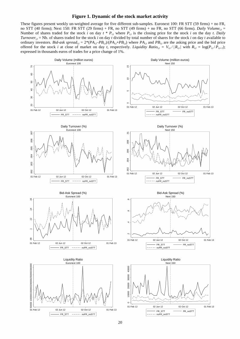
Figures 1-2 show parallel evolution of our dependant variables for stocks included in the

Euronext 100 and the Next 150 indexes. For Euronext 100 and Next 150, we distinguish

between French firms that are subject to STT (FR_STT) and foreign firms that are not subject

to STT (noFR_noSTT). For Next 150, we additionally distinguish French firms that are not

subject to STT (FR_noSTT). The figures show that market liquidity and volatility exhibit

parallel trends before the introduction of the STT, albeit the level is different for different

types of firms. The observation of such parallel trends before introduction of the tax allows us

to make a counterfactual assumption that our variables of interest would preserve these trends

if the tax had not applied.

20

Figure 1. Dynamic of the stock market activity

These figures present weekly un-weighted average for five different sub-samples. Euronext 100: FR STT (59 firms) + no FR, no STT (40 firms); Next 150: FR STT (29 firms) + FR, no STT (49 firms) + no FR, no STT (66 firms). Daily Volumei,t = Number of shares traded for the stock i on day t * Pi,t where Pi,t is the closing price for the stock i on the day t. Daily Turnoveri,t = Nb. of shares traded for the stock i on day t divided by total number of shares for the stock i on day t available to ordinary investors. Bid-ask spreadi,t = 2*(PAi,t–PBi,t)/(PAi,t+PBi,t) where PAi,t and PBi,t are the asking price and the bid price offered for the stock i at close of market on day t, respectively. Liquidity Ratioi,t = Vi,t / |

Ri,t | with Ri,t = log(Pi,t / Pi,t–1);

expressed in thousands euros of trades for a price change of 1%.

2030

40

5060

70

01 Feb 12 02 Jun 12 02 Oct 12 01 Feb 13

FR_STT noFR_noSTT

Euronext 100Daily Volume (million euros)

05

101

5

01 Feb 12 02 Jun 12 02 Oct 12 01 Feb 13

FR_STT FR_noSTTnoFR_noSTT

Next 150Daily Volume (million euros)

.002

.00

3.0

04.0

05

.006

.007

01 Feb 12 02 Jun 12 02 Oct 12 01 Feb 13

FR_STT noFR_noSTT

Euronext 100Daily Turnover (%)

.00

2.0

04

.00

6.0

08.0

1

01 Feb 12 02 Jun 12 02 Oct 12 01 Feb 13


Next 150Daily Turnover (%)

.08

.1.1

2.1

4.1

6

01 Feb 12 02 Jun 12 02 Oct 12 01 Feb 13

FR_STT noFR_noSTT

Euronext 100Bid-Ask Spread (%)

.2.4

.6.8

01 Feb 12 02 Jun 12 02 Oct 12 01 Feb 13


Next 150Bid-Ask Spread (%)

5000

010

000

0150

0002

0000

0250

000

300

000

01 Feb 12 02 Jun 12 02 Oct 12 01 Feb 13

FR_STT noFR_noSTT

Euronext 100Liquidity Ratio

01

0000

2000

030

000

400

00

01 Feb 12 02 Jun 12 02 Oct 12 01 Feb 13


Next 150Liquidity Ratio

21

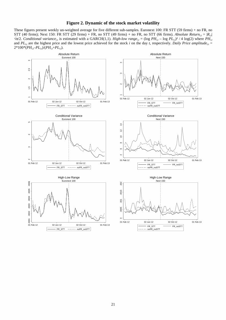
Figure 2. Dynamic of the stock market volatility

These figures present weekly un-weighted average for five different sub-samples. Euronext 100: FR STT (59 firms) + no FR, no STT (40 firms); Next 150: FR STT (29 firms) + FR, no STT (49 firms) + no FR, no STT (66 firms). Absolute Returni,t = |Ri,t| √π/2. Conditional variancei,t is estimated with a GARCH(1,1). High-low rangei,t = (log PHi,t – log PLi,t)² / 4 log(2) where PHi,t and PLi,t are the highest price and the lowest price achieved for the stock i on the day t, respectively. Daily Price amplitudei,t = 2*100*(PHi,t–PLi,t)/(PHi,t+PLi,t).

11.

52

2.5

3

01 Feb 12 02 Jun 12 02 Oct 12 01 Feb 13

FR_STT noFR_noSTT

Euronext 100Absolute Return

12

34

01 Feb 12 02 Jun 12 02 Oct 12 01 Feb 13


Next 150Absolute Return

23

45

01 Feb 12 02 Jun 12 02 Oct 12 01 Feb 13

FR_STT noFR_noSTT

Euronext 100Conditional Variance

46

810

12

14

01 Feb 12 02 Jun 12 02 Oct 12 01 Feb 13


Next 150Conditional Variance

.000

1.0

002

.00

03.0

004

.000

5.0

006

01 Feb 12 02 Jun 12 02 Oct 12 01 Feb 13

FR_STT noFR_noSTT

Euronext 100High-Low Range

0.0

005

.001

.001

5.0

02

01 Feb 12 02 Jun 12 02 Oct 12 01 Feb 13


Next 150High-Low Range

22

4.2. Difference-in-difference results

We estimate the impact of the introduction of the STT on market quality and present results of

difference-in-difference estimation in Tables 4-5. Estimation is done for three different

subsamples that differ with respect to treatment and control group. In column 1, we present

results for stocks included in the Euronext 100 index, whereas in columns 2-3 – for stocks in

Next 150 index. The control group consists of foreign stocks in columns 1 and 3 and of

French stocks that are not subject to the STT in column 2 (see section 3.2 for more details

about subsamples).

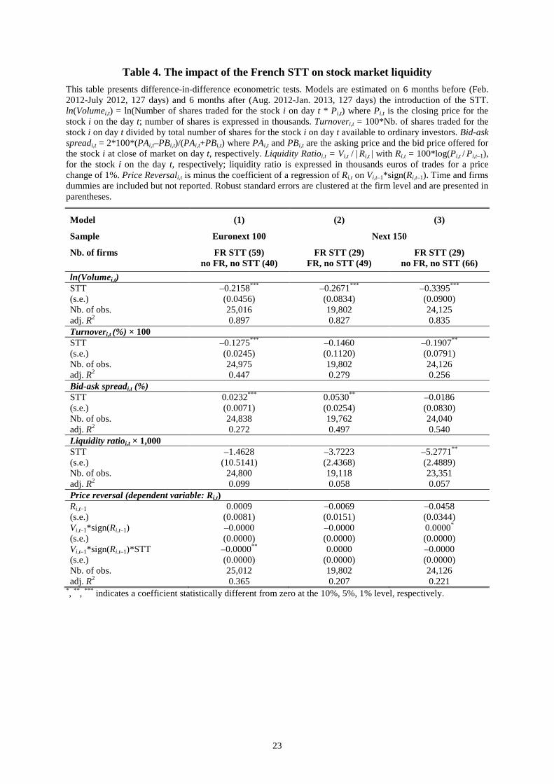
Table 4 presents results for liquidity measured by volume, turnover, bid-ask spread, liquidity

ratio and price reversal (see section 3.3 for definitions). The results show that the introduction

of the STT has reduced market volume and turnover of stocks subject to the STT relatively to

control groups. The coefficients are not only statistically significant in all three subsamples

but also economically meaningful. According to coefficients in columns 1-3, volumes have

declined by 19%, 23% and 29% (corresponding to the coefficients of -0.2159, -0.2671 and -

0.3395).28 There is also evidence that transaction costs have gone up as the bid-ask spread has

increased. This result holds for the subsamples in columns 1-2, but is not robust for the

sample of large French midcaps with other foreign firms as a control group (column 3).

This decrease in volume and the (possible) increase of bid-ask spreads should be put into their

historical context as stock market development worldwide has been tremendous. Since 1990,

the value of share trading at the Bourse de Paris has increased by approximately 2 000%, that

is an increase of 50% on average per year (see Figure B - Panel A in appendix). This trend is

similar in most of the Western countries. Moreover, the value of share trading might vary

considerably from one year to another depending on economic situation. In 1997 and 2000,

for instance, market volume increased by 75% compared to the previous year; in 2009 it

decreased by almost 50% (see Figure B - Panel B in appendix). At the same time, there is a

sharp downward trend in financial market transaction costs. Comerton-Forde, Hendershott,

Jones, Moulton, and Seasholes (2010) report, for instance, that the value-weighted effective

spread in the NYSE was divided by ten between 1994 and 2005.

28 Since transaction tax is levied on volumes, this is translated in the tax base decline of the same magnitude.

23

Table 4. The impact of the French STT on stock market liquidity

This table presents difference-in-difference econometric tests. Models are estimated on 6 months before (Feb. 2012-July 2012, 127 days) and 6 months after (Aug. 2012-Jan. 2013, 127 days) the introduction of the STT. ln(Volumei,t) = ln(Number of shares traded for the stock i on day t * Pi,t) where Pi,t is the closing price for the stock i on the day t; number of shares is expressed in thousands. Turnoveri,t = 100*Nb. of shares traded for the stock i on day t divided by total number of shares for the stock i on day t available to ordinary investors. Bid-ask spreadi,t = 2*100*(PAi,t–PBi,t)/(PAi,t+PBi,t) where PAi,t and PBi,t are the asking price and the bid price offered for the stock i at close of market on day t, respectively. Liquidity Ratioi,t = Vi,t / |

Ri,t | with Ri,t = 100*log(Pi,t / Pi,t–1),

for the stock i on the day t, respectively; liquidity ratio is expressed in thousands euros of trades for a price change of 1%. Price Reversali,t is minus the coefficient of a regression of Ri,t on Vi,t–1*sign(Ri,t–1). Time and firms dummies are included but not reported. Robust standard errors are clustered at the firm level and are presented in parentheses.

Model (1) (2) (3)

Sample Euronext 100 Next 150

Nb. of firms FR STT (59) no FR, no STT (40)

FR STT (29) FR, no STT (49)

FR STT (29) no FR, no STT (66)

ln(Volumei,t) STT –0.2158*** –0.2671*** –0.3395*** (s.e.) (0.0456) (0.0834) (0.0900) Nb. of obs. 25,016 19,802 24,125 adj. R2 0.897 0.827 0.835 Turnoveri,t (%) × 100 STT –0.1275*** –0.1460 –0.1907** (s.e.) (0.0245) (0.1120) (0.0791) Nb. of obs. 24,975 19,802 24,126 adj. R2 0.447 0.279 0.256 Bid-ask spreadi,t (%) STT 0.0232*** 0.0530** –0.0186 (s.e.) (0.0071) (0.0254) (0.0830) Nb. of obs. 24,838 19,762 24,040 adj. R2 0.272 0.497 0.540 Liquidity ratioi,t × 1,000 STT –1.4628 –3.7223 –5.2771** (s.e.) (10.5141) (2.4368) (2.4889) Nb. of obs. 24,800 19,118 23,351 adj. R2 0.099 0.058 0.057 Price reversal (dependent variable: Ri,t) Ri,t–1 0.0009 –0.0069 –0.0458 (s.e.) (0.0081) (0.0151) (0.0344) Vi,t–1*sign(Ri,t–1) –0.0000 –0.0000 0.0000* (s.e.) (0.0000) (0.0000) (0.0000) Vi,t–1*sign(Ri,t–1)*STT –0.0000** 0.0000 –0.0000 (s.e.) (0.0000) (0.0000) (0.0000) Nb. of obs. 25,012 19,802 24,126 adj. R2 0.365 0.207 0.221

*, ** , *** indicates a coefficient statistically different from zero at the 10%, 5%, 1% level, respectively.

24

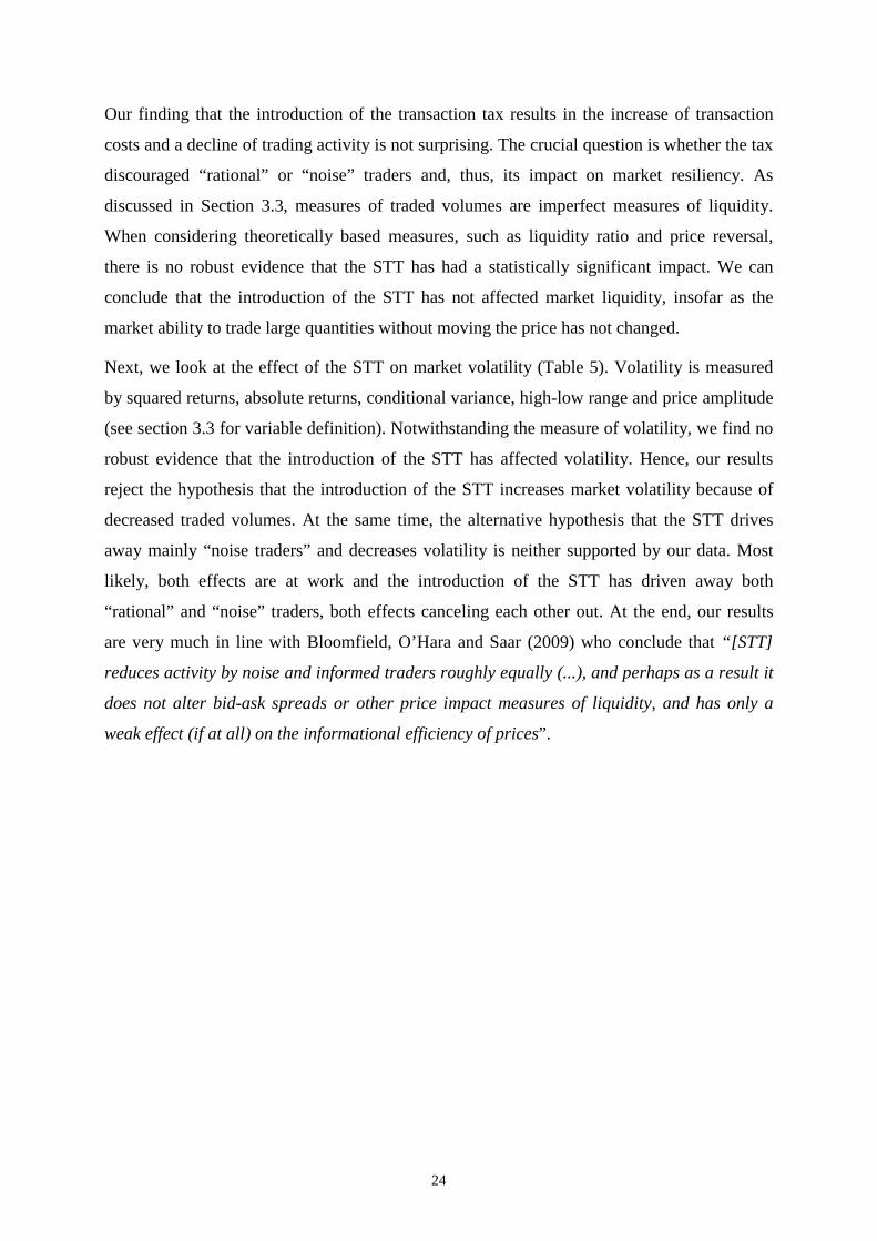
Our finding that the introduction of the transaction tax results in the increase of transaction

costs and a decline of trading activity is not surprising. The crucial question is whether the tax

discouraged “rational” or “noise” traders and, thus, its impact on market resiliency. As

discussed in Section 3.3, measures of traded volumes are imperfect measures of liquidity.

When considering theoretically based measures, such as liquidity ratio and price reversal,

there is no robust evidence that the STT has had a statistically significant impact. We can

conclude that the introduction of the STT has not affected market liquidity, insofar as the

market ability to trade large quantities without moving the price has not changed.

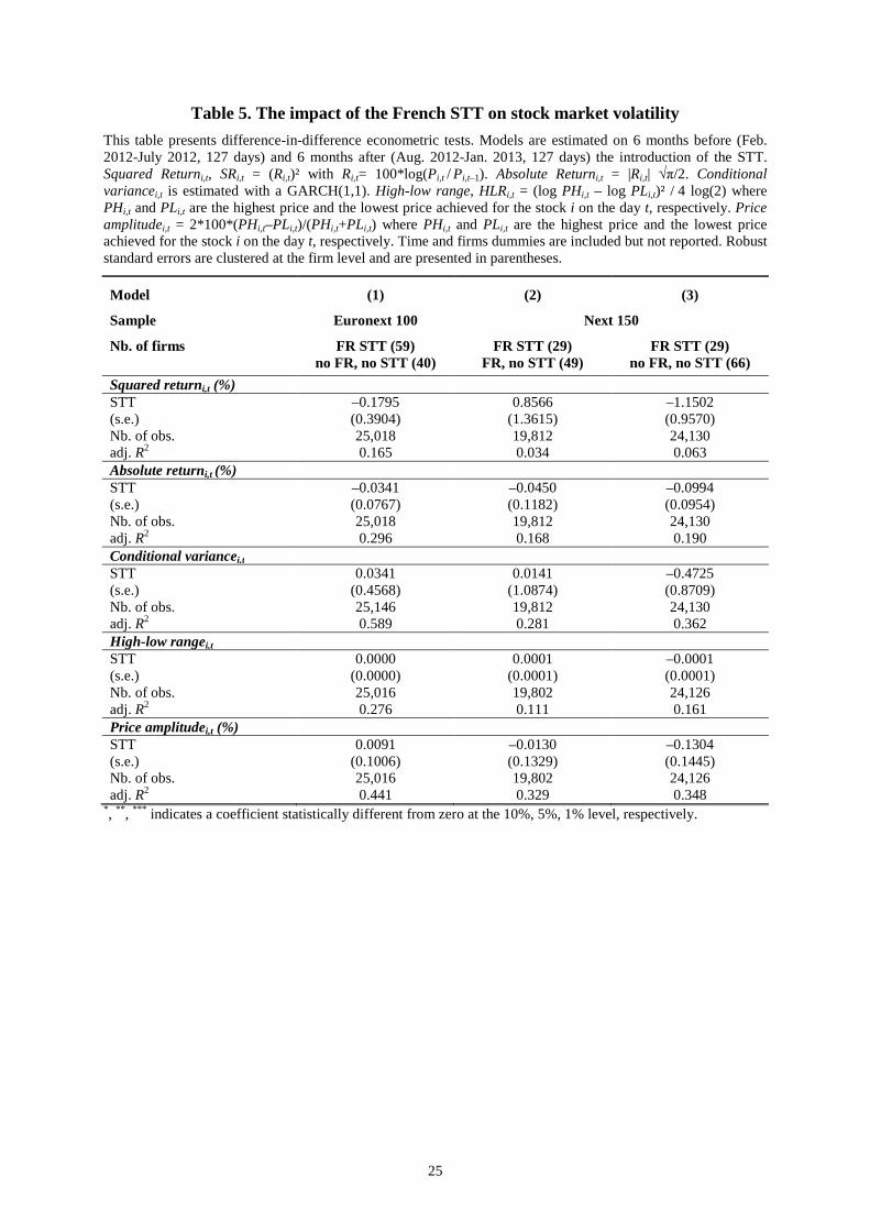
Next, we look at the effect of the STT on market volatility (Table 5). Volatility is measured

by squared returns, absolute returns, conditional variance, high-low range and price amplitude

(see section 3.3 for variable definition). Notwithstanding the measure of volatility, we find no

robust evidence that the introduction of the STT has affected volatility. Hence, our results

reject the hypothesis that the introduction of the STT increases market volatility because of

decreased traded volumes. At the same time, the alternative hypothesis that the STT drives

away mainly “noise traders” and decreases volatility is neither supported by our data. Most

likely, both effects are at work and the introduction of the STT has driven away both

“rational” and “noise” traders, both effects canceling each other out. At the end, our results

are very much in line with Bloomfield, O’Hara and Saar (2009) who conclude that “[STT]

reduces activity by noise and informed traders roughly equally (...), and perhaps as a result it

does not alter bid-ask spreads or other price impact measures of liquidity, and has only a

weak effect (if at all) on the informational efficiency of prices”.

25

Table 5. The impact of the French STT on stock market volatility

This table presents difference-in-difference econometric tests. Models are estimated on 6 months before (Feb. 2012-July 2012, 127 days) and 6 months after (Aug. 2012-Jan. 2013, 127 days) the introduction of the STT. Squared Returni,t, SRi,t = (Ri,t)² with Ri,t= 100*log(Pi,t / Pi,t–1). Absolute Returni,t = |Ri,t| √π/2. Conditional variancei,t is estimated with a GARCH(1,1). High-low range, HLRi,t = (log PHi,t – log PLi,t)² / 4 log(2) where PHi,t and PLi,t are the highest price and the lowest price achieved for the stock i on the day t, respectively. Price amplitudei,t = 2*100*(PHi,t–PLi,t)/(PHi,t+PLi,t) where PHi,t and PLi,t are the highest price and the lowest price achieved for the stock i on the day t, respectively. Time and firms dummies are included but not reported. Robust standard errors are clustered at the firm level and are presented in parentheses.

Model (1) (2) (3)





Squared returni,t (%) STT –0.1795 0.8566 –1.1502 (s.e.) (0.3904) (1.3615) (0.9570) Nb. of obs. 25,018 19,812 24,130 adj. R2 0.165 0.034 0.063 Absolute returni,t (%) STT –0.0341 –0.0450 –0.0994 (s.e.) (0.0767) (0.1182) (0.0954) Nb. of obs. 25,018 19,812 24,130 adj. R2 0.296 0.168 0.190 Conditional variancei,t STT 0.0341 0.0141 –0.4725 (s.e.) (0.4568) (1.0874) (0.8709) Nb. of obs. 25,146 19,812 24,130 adj. R2 0.589 0.281 0.362 High-low rangei,t STT 0.0000 0.0001 –0.0001 (s.e.) (0.0000) (0.0001) (0.0001) Nb. of obs. 25,016 19,802 24,126 adj. R2 0.276 0.111 0.161 Price amplitudei,t (%) STT 0.0091 –0.0130 –0.1304 (s.e.) (0.1006) (0.1329) (0.1445) Nb. of obs. 25,016 19,802 24,126 adj. R2 0.441 0.329 0.348


26

5. Robustness checks

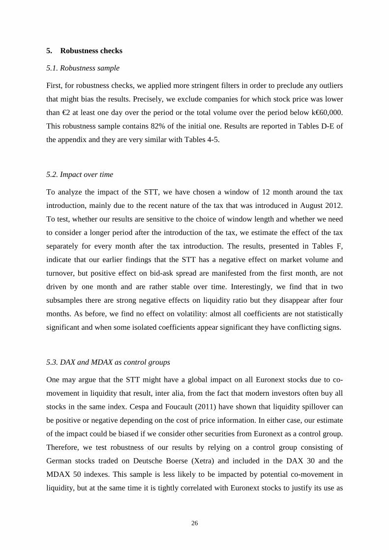
5.1. Robustness sample

First, for robustness checks, we applied more stringent filters in order to preclude any outliers

that might bias the results. Precisely, we exclude companies for which stock price was lower

than €2 at least one day over the period or the total volume over the period below k€60,000.

This robustness sample contains 82% of the initial one. Results are reported in Tables D-E of

the appendix and they are very similar with Tables 4-5.

5.2. Impact over time

To analyze the impact of the STT, we have chosen a window of 12 month around the tax

introduction, mainly due to the recent nature of the tax that was introduced in August 2012.

To test, whether our results are sensitive to the choice of window length and whether we need

to consider a longer period after the introduction of the tax, we estimate the effect of the tax

separately for every month after the tax introduction. The results, presented in Tables F,

indicate that our earlier findings that the STT has a negative effect on market volume and

turnover, but positive effect on bid-ask spread are manifested from the first month, are not

driven by one month and are rather stable over time. Interestingly, we find that in two

subsamples there are strong negative effects on liquidity ratio but they disappear after four

months. As before, we find no effect on volatility: almost all coefficients are not statistically

significant and when some isolated coefficients appear significant they have conflicting signs.

5.3. DAX and MDAX as control groups

One may argue that the STT might have a global impact on all Euronext stocks due to co-

movement in liquidity that result, inter alia, from the fact that modern investors often buy all

stocks in the same index. Cespa and Foucault (2011) have shown that liquidity spillover can

be positive or negative depending on the cost of price information. In either case, our estimate

of the impact could be biased if we consider other securities from Euronext as a control group.

Therefore, we test robustness of our results by relying on a control group consisting of

German stocks traded on Deutsche Boerse (Xetra) and included in the DAX 30 and the

MDAX 50 indexes. This sample is less likely to be impacted by potential co-movement in

liquidity, but at the same time it is tightly correlated with Euronext stocks to justify its use as

27

a control group (see Table 2).

Results of difference-in-difference estimation are presented in Tables G-H. In column 1, the

sample consists of largest French stocks in Euronext 100 (treated group) and largest German

stocks in DAX (control group). In column 2, the sample covers mid-cap French stocks in Next

150 (treated group) and mid-cap German stocks in MDAX (control group). Both samples

confirm our earlier findings. The introduction of the STT always has a negative effect on

market volume and there is also evidence that it might increase the bid-ask spread. At the

same time, the effect on liquidity ratio is insignificant, meaning that markets are sufficiently

liquid to be able to absorb large market transactions without any price effects. Finally, there is

no effect on volatility.

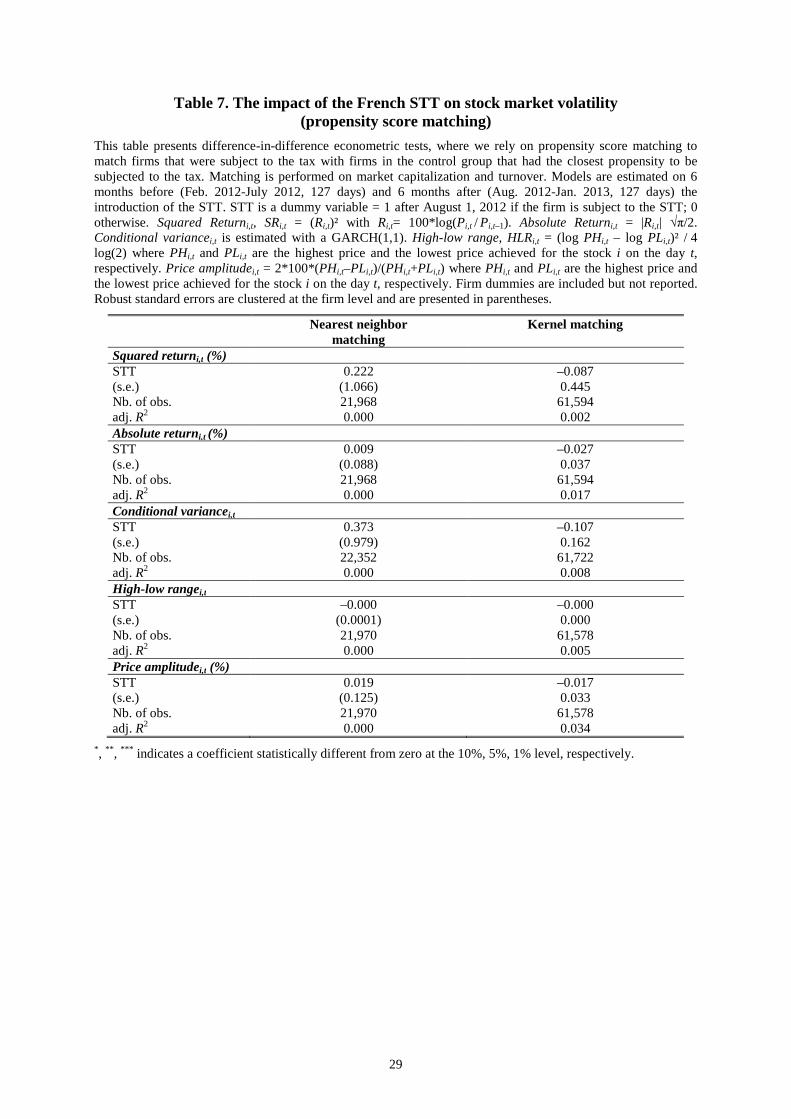
5.4. Propensity score matching

To further improve the quality of the control group, we rely on propensity score matching.

This will allow us to compare stocks that were subjected to a STT with comparable (foreign

and French) stocks listed on Euronext that were not subjected to a tax. In order to determine

“comparable” stocks we compute average market capitalization and turnover of stocks

included in Euronex 100 and Next 150 before the introduction of the STT and then run a

logistic regression, where a probability of a stock being subjected to a tax is a function of

these observable characteristics (market capitalization, turnover and volatility). The choice of

the first two variables follows Foucault et al. (2011) and we augment the model with an

additional volatility measure (squared returns, conditional variance, high-low range). We

assure that all variables in the model are statistically significant, because we rely on model

coefficients to assign to each stock a probability of being taxed and then match stocks

subjected to the STT with stocks that were the “closest” in terms of the propensity score. We

test robustness of our results with “the nearest neighbor” and “Kernel” matching. In the

second step, we compare the performance of the taxed stocks with the matched stocks that

were not subjected to STT by estimating the following econometric model:

�� − ��

= �� + �� + �� + �� + ��.

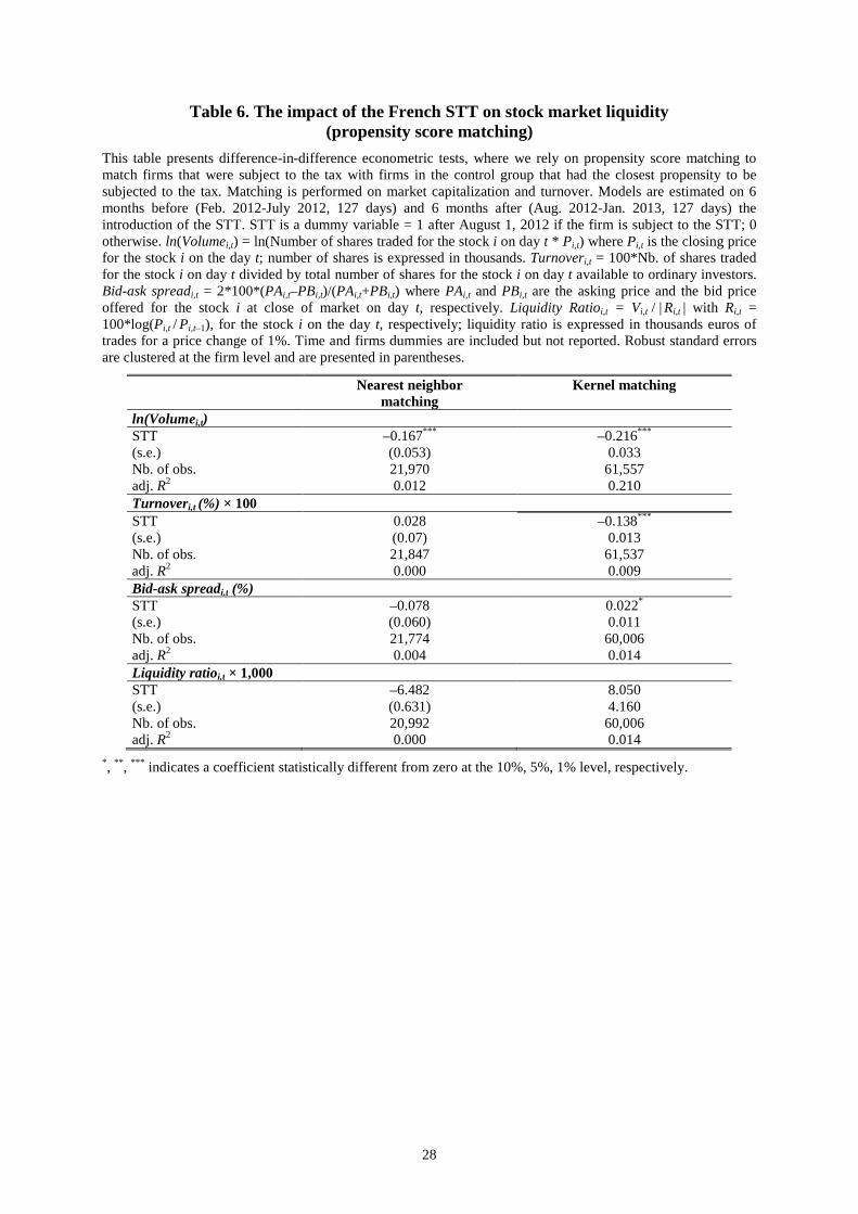
Estimation results, presented in Tables 6-7, confirm our earlier findings that the introduction

of the STT always has a negative effect on market volume, but no effect on market liquidity

or volatility. Similar to our earlier findings, a negative effect on market turnover and a

positive effect on bid-ask spread is not always robust.

28

Table 6. The impact of the French STT on stock market liquidity (propensity score matching)

This table presents difference-in-difference econometric tests, where we rely on propensity score matching to match firms that were subject to the tax with firms in the control group that had the closest propensity to be subjected to the tax. Matching is performed on market capitalization and turnover. Models are estimated on 6 months before (Feb. 2012-July 2012, 127 days) and 6 months after (Aug. 2012-Jan. 2013, 127 days) the introduction of the STT. STT is a dummy variable = 1 after August 1, 2012 if the firm is subject to the STT; 0 otherwise. ln(Volumei,t) = ln(Number of shares traded for the stock i on day t * Pi,t) where Pi,t is the closing price for the stock i on the day t; number of shares is expressed in thousands. Turnoveri,t = 100*Nb. of shares traded for the stock i on day t divided by total number of shares for the stock i on day t available to ordinary investors. Bid-ask spreadi,t = 2*100*(PAi,t–PBi,t)/(PAi,t+PBi,t) where PAi,t and PBi,t are the asking price and the bid price offered for the stock i at close of market on day t, respectively. Liquidity Ratioi,t = Vi,t / |

Ri,t | with Ri,t =

100*log(Pi,t / Pi,t–1), for the stock i on the day t, respectively; liquidity ratio is expressed in thousands euros of trades for a price change of 1%. Time and firms dummies are included but not reported. Robust standard errors are clustered at the firm level and are presented in parentheses.

Nearest neighbor matching

Kernel matching

ln(Volumei,t)

STT –0.167*** –0.216*** (s.e.) (0.053) 0.033 Nb. of obs. 21,970 61,557 adj. R2 0.012 0.210 Turnoveri,t (%) × 100 STT 0.028 –0.138*** (s.e.) (0.07) 0.013 Nb. of obs. 21,847 61,537 adj. R2 0.000 0.009 Bid-ask spreadi,t (%) STT –0.078 0.022* (s.e.) (0.060) 0.011 Nb. of obs. 21,774 60,006 adj. R2 0.004 0.014 Liquidity ratioi,t × 1,000 STT –6.482 8.050 (s.e.) (0.631) 4.160 Nb. of obs. 20,992 60,006 adj. R2 0.000 0.014


29

Table 7. The impact of the French STT on stock market volatility (propensity score matching)

This table presents difference-in-difference econometric tests, where we rely on propensity score matching to match firms that were subject to the tax with firms in the control group that had the closest propensity to be subjected to the tax. Matching is performed on market capitalization and turnover. Models are estimated on 6 months before (Feb. 2012-July 2012, 127 days) and 6 months after (Aug. 2012-Jan. 2013, 127 days) the introduction of the STT. STT is a dummy variable = 1 after August 1, 2012 if the firm is subject to the STT; 0 otherwise. Squared Returni,t, SRi,t = (Ri,t)² with Ri,t= 100*log(Pi,t / Pi,t–1). Absolute Returni,t = |Ri,t| √π/2. Conditional variancei,t is estimated with a GARCH(1,1). High-low range, HLRi,t = (log PHi,t – log PLi,t)² / 4 log(2) where PHi,t and PLi,t are the highest price and the lowest price achieved for the stock i on the day t, respectively. Price amplitudei,t = 2*100*(PHi,t–PLi,t)/(PHi,t+PLi,t) where PHi,t and PLi,t are the highest price and the lowest price achieved for the stock i on the day t, respectively. Firm dummies are included but not reported. Robust standard errors are clustered at the firm level and are presented in parentheses.

Nearest neighbor matching

Kernel matching

Squared returni,t (%)

STT 0.222 –0.087 (s.e.) (1.066) 0.445 Nb. of obs. 21,968 61,594 adj. R2 0.000 0.002 Absolute returni,t (%) STT 0.009 –0.027 (s.e.) (0.088) 0.037 Nb. of obs. 21,968 61,594 adj. R2 0.000 0.017 Conditional variancei,t STT 0.373 –0.107 (s.e.) (0.979) 0.162 Nb. of obs. 22,352 61,722 adj. R2 0.000 0.008 High-low rangei,t STT –0.000 –0.000 (s.e.) (0.0001) 0.000 Nb. of obs. 21,970 61,578 adj. R2 0.000 0.005 Price amplitudei,t (%) STT 0.019 –0.017 (s.e.) (0.125) 0.033 Nb. of obs. 21,970 61,578 adj. R2 0.000 0.034


30

6. Conclusion

This paper analyzes the impact of financial transaction taxes on market volatility. This

question is at the heart of economic policy debate about the use of financial transaction taxes

to curb speculative activity and render financial markets more stable. In contrast, the

opponents argue that taxation of financial transactions will hurt market liquidity, thus, making

markets even more volatile.

Since theoretical predictions on this subject are ambiguous, there is a need for an econometric

analysis. Although a number of papers empirically examine the impact of STT, there is no

paper that can make a strong case for a causal relationship between STT and volatility. Most

of these studies do not address endogeneity problems inasmuch as they cannot isolate the

impact of the STT from other economic developments during the same time period.

In this paper, we study the impact of the STT introduction in France in 2012 on market

liquidity and volatility. Unlike previous studies, we are able to isolate the effect of the tax due

to the unique design of the French STT. As the tax is levied only on large French firms traded

on Euronext, this provides us with two control groups (smaller French firms and foreign

firms) and allows us to use difference-in-difference methodology. Our results show that the

introduction of the STT has reduced volume and turnover of stocks and increased bid-ask

spreads. At the same time, we find no effect on theoretically based measures of liquidity, such

as price impact. As to volatility measures, the results are mostly insignificant. Our results are

robust to a number of robustness tests that include different control groups, dynamic effects

and propensity score matching.

To sum up, our investigation shows that STT is neither a panacea nor a “madness” for

financial markets. Our results do not confirm expectations that STT decreases market

volatility by curbing speculative activity, but at the same time, there is no significant effect on

market volatility and even liquidity.

31

References

Amihud, Y., 2002, Illiquidity and stock returns: Cross-section and time-series effects, Journal of Financial Markets, 5, 31-56.

Amihud, Y., and Mendelson, H., 2003, Effects of a New York State Stock Transaction Tax, Unpublished manuscript, New York University.

Baltagi, B., Li, D. and Li, Q., 2006, Transaction Tax and Stock Market Behavior: Evidence from an Emerging Market, Empirical Economics, 31, 393-408.

Beach, W.E., 1939, Stock Market Continuity, The American Economic Review, 29(4), 774-789.

Becchetti, L., M. Ferrari and U. Trenta, 2013, The impact of the French Tobin tax, CEIS Working paper, No. 266.

Bertrand, M., E. Duflo and S. Mullainathan, 2004, How Much Should We Trust Differences-in-Differences Estimates?, Quarterly Journal of Economics 119(1), 249-275.

Bloomfield, R., M. O’Hara, and G. Saar, 2009, How Noise Trading Affects Markets: An Experimental Analysis, Review of Financial Studies, 22(6), 2275-2302.

Brandt, M.W. and F.X. Diebold, 2006, A no-arbitrage approach to range-based estimation of return covariances and correlations, Journal of Business, 79, 61-74.

Campbell, J., S. Grossman, and J. Wang, 1993, Trading volume and serial correlation in stock returns, Quarterly Journal of Economics, 108, 905-939.

Cespa, G., and Th. Foucault, 2011, Learning from Prices, Liquidity Spillovers, and Market Segmentation, Working paper.

Chou, R. K., and G. H. K. Wang, 2006, Transaction tax and market quality of the Taiwan stock index futures, Journal of Futures Markets 26(12), 1195-1216.

Colliard, J.E., and P. Hoffmann, 2013, Sand in the chips: Evidence on taxing transactions in an electronic market, mimeo.

Comerton-Forde, C., T. Hendershott, Ch. Jones, P. Moulton, and M. Seasholes, 2010, Time variation in liquidity: The role of market-maker inventories and revenues, Journal of Finance, 65, 295-331.

Dolley, J.C., 1938, The Effect of Government Regulation in the Stock-trading volume of the New York Stock Exchange, The American Economic Review, 28(1), 8-26.

Dooley, M.P., 1996, Tobin Tax: Good Theory, Weak Evidence, Questionable Policy, in “The Tobin Tax: Coping with Financial Volatility”, M. ul Haq, I. Kaul, and I. Grunberg. Oxford University Press.

Ehrenstein, G., F. Westerhoff and D. Stauffer, 2005, Tobin Tax and Market Depth, Quantitative Finance,5(2), 213-18.

Eichengreen, B., J. Tobin, and Ch. Wyplosz, 1995, Two Cases for Sand in the Wheels of International Finance, Economic Journal, 105, 162-172.

Engle, R.F., and Gallo, G.M., 2006, A Multiple Indicators Model for Volatility Using Intra-Daily Data, Journal of Econometrics, 131(1-2), 3-27.

Foucault, T., D. Sraer and D.J. Thesmar, 2011, Individual Investors and Volatility, Journal of Finance, 66(4), 1369-1406.

32

Fu, Y., W. Qian, and B. Yeung, 2013, Speculative Investors and Tobin’s Tax in the Housing Market, NBER Working Paper, No. 19400.

Gabor, D., 2013, A step too far? The European Financial Transactions Tax and Shadow Banking, Working paper.

Gabrielsen, A., M. Marzo and P. Zagaglia, 2011, Measuring market liquidity: An introductory survey, Working paper.

Haberer, M., 2004, Might a Securities Transaction Tax Mitigate Excess Volatility? Some Evidence from the Literature, CoFE Discussion Paper 04-06, Konstanz: Center of Finance and Econometrics, University of Konstanz.

Haferkorn, M., and K. Zimmermann, 2013, Securities Transaction Tax and Market Quality: The Case of France, Goethe University Frankfurt, mimeo.

Hau, H., 1998, Competitive Entry and Endogenous Risk in the Foreign Exchange Market, Review of Financial Studies 11(4), 757-87.

Hau, H., 2006, The role of transaction costs for financial volatility: Evidence from the Paris bourse, Journal of The European Economic Association, 4(4), 862-890.

Hu, S., 1998, The Effects of the Stock Transaction Tax on the Stock Market: Experience from Asian Markets, Pacific Basin Finance Journal, 6, 347-64.

Jones, C.M. and Seguin, P.J., 1997, Transaction Costs and Price Volatility: Evidence from Commission Deregulation, The American Economic Review, 87(4), 728-37.

Keynes, J.M., 1936, The general theory of employment, interest, and money. New York: Harcourt Brace.

Kupiec, P., 1996, Noise Traders, Excess Volatility, and a Securities Transaction Tax, Journal of Financial Services Research, 10, 115-29.

Liau Y.-S., Y.-C. Wu and H. Hsu, 2012, Transaction tax and market volatility: Evidence from the Taiwan futures market, Journal of Applied Finance & Banking, 2(2), 45-58.

Liu, S., 2007, Securities Transaction Tax and Market Efficiency: Evidence from the Japanese Experience, Journal of Financial Services Research, 32, 161-76.

Matheson, T., 2011, Taxing Financial Transactions: Issues and Evidence, IMF Working paper, WP/11/54.

Mannaro, K., M. Marchesi, and A. Setzu, 2008, Using an Artificial Financial Market for Assessing the Impact of Tobin-Like Transaction Taxes, Journal of Economic Behavior and Organization, 67(2), 445-62

McCulloch, N., and G. Pacillo, 2011, The Tobin Tax: A Review of the Evidence, IDS Research Report, n°68, Institute of Development Studies.

Meyer, S., M. Wagener and Ch. Weinhardt, 2013, Politically Motivated Taxes in Financial Markets: The Case of the French Financial Transaction Tax, Stuttgart Stock Exchange and Karlsruhe Institute of Technology, mimeo.

Niederhoffer, V., and M. Osborne, 1966, Market making and reversal on the stock exchange, Journal of the American Statistical Association, 61, 897-916.

Parkinson, M., 1980, The extreme value method for estimating the variance of the rate of return, Journal of Business, 53, 61-65.

33

Pastor, L., and R. Stambaugh, 2003, Liquidity risk and expected stock returns, Journal of Political Economy 111(3), 642-685.

Phylaktis, K. and A. Aristidou, 2007, Security transaction taxes and financial volatility: Athens stock exchange, Applied Financial Economics, 17(18), 1455-1467.

Pomeranets, A., and D.G. Weaver, 2011, Securities Transaction Taxes and Market Quality, Bank of Canada, Working Paper 2011-26.

Roll, R., 1984, A simple implicit measure of the effective bid-ask spread in an efficient market, Journal of Finance 39, 1127-1139.

Roll, R., 1989, Price Volatility, International Market Links and Their Implication for Regulatory Policies, Journal of Financial Services Research, 3(2-3), 211-46.

Sahu, D., 2008, Does Securities Transaction Tax Distort Market Microstructure? Evidence from Indian Stock Market, Working Paper, Banaras Hindu University.

Saporta, V. and K. Kan, 1997, The effects of stamp duty on the level and volatility of UK equity prices, Bank of England, Working Paper, No. 71.

Sarr, A., and T. Lybek, 2002, Measuring Liquidity in Financial Markets (December 2002). IMF Working Paper, 1-64.

Schwert, G.W., and P.J. Seguin, 1993, Security Transaction Taxes: An Overview of Costs and Benefits and Unresolved Questions, Financial Analysts Journal, 49(5), 27-35.

Song, F.M., and J. Zhang, 2005, Securities transaction tax and market volatility, The Economic Journal, 115(506), 1103-1120.

Stiglitz, J.E., 1989, Using tax policy to curb speculative short-term trading, Journal of Financial Services Research, 3, 101-115.

Subrahmanyam, A., 1998, Transaction taxes and financial market equilibrium, Journal of Business, 71(1), 81-118.

Summers, L.H. and V.P. Summers, 1989, When financial markets work too well: a cautious case for a securities transaction tax, Journal of Financial Services Research, 3, 261-286.

Tobin, J., 1978, A proposal for international monetary reform, Eastern Economic Review, 153-159.

Vayanos, D., and J. Wang, 2012, Market Liquidity: Theory and Empirical Evidence, Handbook of the Economics of Finance.

Umlauf, S.R., 1993, Transaction taxes and the behavior of the Swedish stock market, Journal of Financial Economics, 33, 227-40.

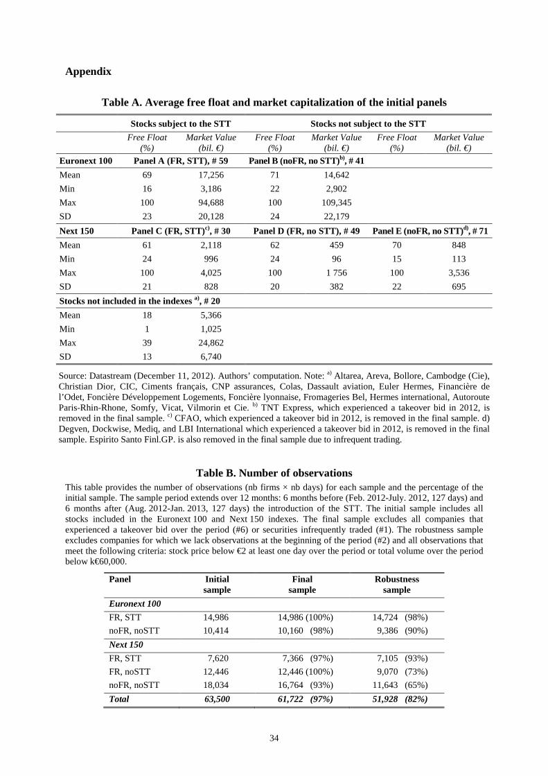
34

Appendix

Table A. Average free float and market capitalization of the initial panels

Stocks subject to the STT Stocks not subject to the STT

Free Float

(%) Market Value

(bil. €) Free Float

(%) Market Value

(bil. €) Free Float

(%) Market Value

(bil. €)

Euronext 100 Panel A (FR, STT), # 59 Panel B (noFR, no STT)b), # 41

Mean 69 17,256 71 14,642

Min 16 3,186 22 2,902

Max 100 94,688 100 109,345

SD 23 20,128 24 22,179

Next 150 Panel C (FR, STT)c), # 30 Panel D (FR, no STT), # 49 Panel E (noFR, no STT)d), # 71

Mean 61 2,118 62 459 70 848

Min 24 996 24 96 15 113

Max 100 4,025 100 1 756 100 3,536

SD 21 828 20 382 22 695

Stocks not included in the indexes a), # 20

Mean 18 5,366

Min 1 1,025

Max 39 24,862

SD 13 6,740

Source: Datastream (December 11, 2012). Authors’ computation. Note: a) Altarea, Areva, Bollore, Cambodge (Cie), Christian Dior, CIC, Ciments français, CNP assurances, Colas, Dassault aviation, Euler Hermes, Financière de l’Odet, Foncière Développement Logements, Foncière lyonnaise, Fromageries Bel, Hermes international, Autoroute Paris-Rhin-Rhone, Somfy, Vicat, Vilmorin et Cie. b) TNT Express, which experienced a takeover bid in 2012, is removed in the final sample. c) CFAO, which experienced a takeover bid in 2012, is removed in the final sample. d) Degven, Dockwise, Mediq, and LBI International which experienced a takeover bid in 2012, is removed in the final sample. Espirito Santo Finl.GP. is also removed in the final sample due to infrequent trading.

Table B. Number of observations This table provides the number of observations (nb firms × nb days) for each sample and the percentage of the initial sample. The sample period extends over 12 months: 6 months before (Feb. 2012-July. 2012, 127 days) and 6 months after (Aug. 2012-Jan. 2013, 127 days) the introduction of the STT. The initial sample includes all stocks included in the Euronext 100 and Next 150 indexes. The final sample excludes all companies that experienced a takeover bid over the period (#6) or securities infrequently traded (#1). The robustness sample excludes companies for which we lack observations at the beginning of the period (#2) and all observations that meet the following criteria: stock price below €2 at least one day over the period or total volume over the period below k€60,000.

Panel Initial sample

Final sample

Robustness sample

Euronext 100

FR, STT 14,986 14,986 (100%) 14,724 (98%)

noFR, noSTT 10,414 10,160 (98%) 9,386 (90%)

Next 150

FR, STT 7,620 7,366 (97%) 7,105 (93%)

FR, noSTT 12,446 12,446 (100%) 9,070 (73%)

noFR, noSTT 18,034 16,764 (93%) 11,643 (65%)

Total 63,500 61,722 (97%) 51,928 (82%)

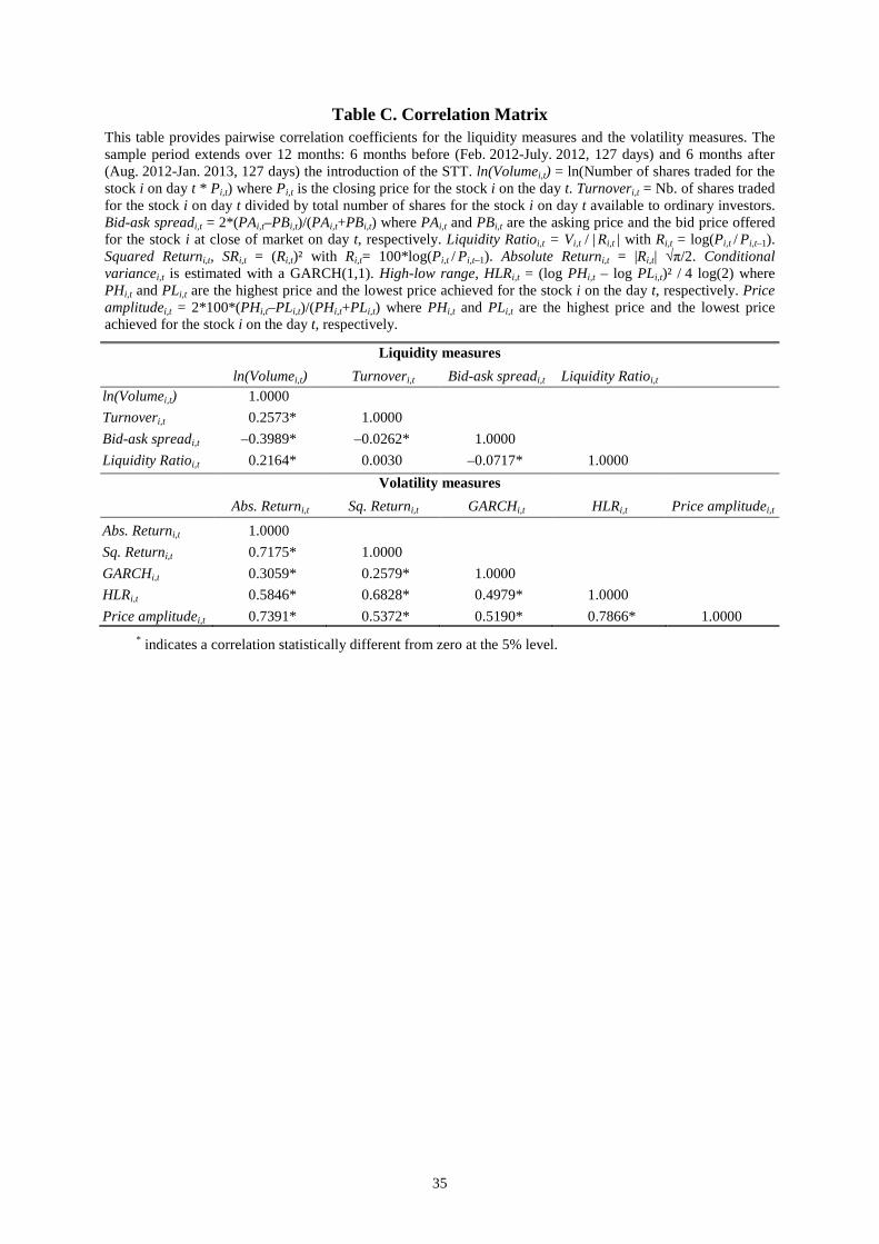
35

Table C. Correlation Matrix This table provides pairwise correlation coefficients for the liquidity measures and the volatility measures. The sample period extends over 12 months: 6 months before (Feb. 2012-July. 2012, 127 days) and 6 months after (Aug. 2012-Jan. 2013, 127 days) the introduction of the STT. ln(Volumei,t) = ln(Number of shares traded for the stock i on day t * Pi,t) where Pi,t is the closing price for the stock i on the day t. Turnoveri,t = Nb. of shares traded for the stock i on day t divided by total number of shares for the stock i on day t available to ordinary investors. Bid-ask spreadi,t = 2*(PAi,t–PBi,t)/(PAi,t+PBi,t) where PAi,t and PBi,t are the asking price and the bid price offered for the stock i at close of market on day t, respectively. Liquidity Ratioi,t = Vi,t / |

Ri,t | with Ri,t = log(Pi,t / Pi,t–1).

Squared Returni,t, SRi,t = (Ri,t)² with Ri,t= 100*log(Pi,t / Pi,t–1). Absolute Returni,t = |Ri,t| √π/2. Conditional variancei,t is estimated with a GARCH(1,1). High-low range, HLRi,t = (log PHi,t – log PLi,t)² / 4 log(2) where PHi,t and PLi,t are the highest price and the lowest price achieved for the stock i on the day t, respectively. Price amplitudei,t = 2*100*(PHi,t–PLi,t)/(PHi,t+PLi,t) where PHi,t and PLi,t are the highest price and the lowest price achieved for the stock i on the day t, respectively.

Liquidity measures

ln(Volumei,t) Turnoveri,t Bid-ask spreadi,t Liquidity Ratioi,t ln(Volumei,t) 1.0000

Turnoveri,t 0.2573* 1.0000

Bid-ask spreadi,t –0.3989* –0.0262* 1.0000

Liquidity Ratioi,t 0.2164* 0.0030 –0.0717* 1.0000

Volatility measures

Abs. Returni,t Sq. Returni,t GARCHi,t HLRi,t Price amplitudei,t

Abs. Returni,t 1.0000

Sq. Returni,t 0.7175* 1.0000

GARCHi,t 0.3059* 0.2579* 1.0000

HLRi,t 0.5846* 0.6828* 0.4979* 1.0000

Price amplitudei,t 0.7391* 0.5372* 0.5190* 0.7866* 1.0000

* indicates a correlation statistically different from zero at the 5% level.

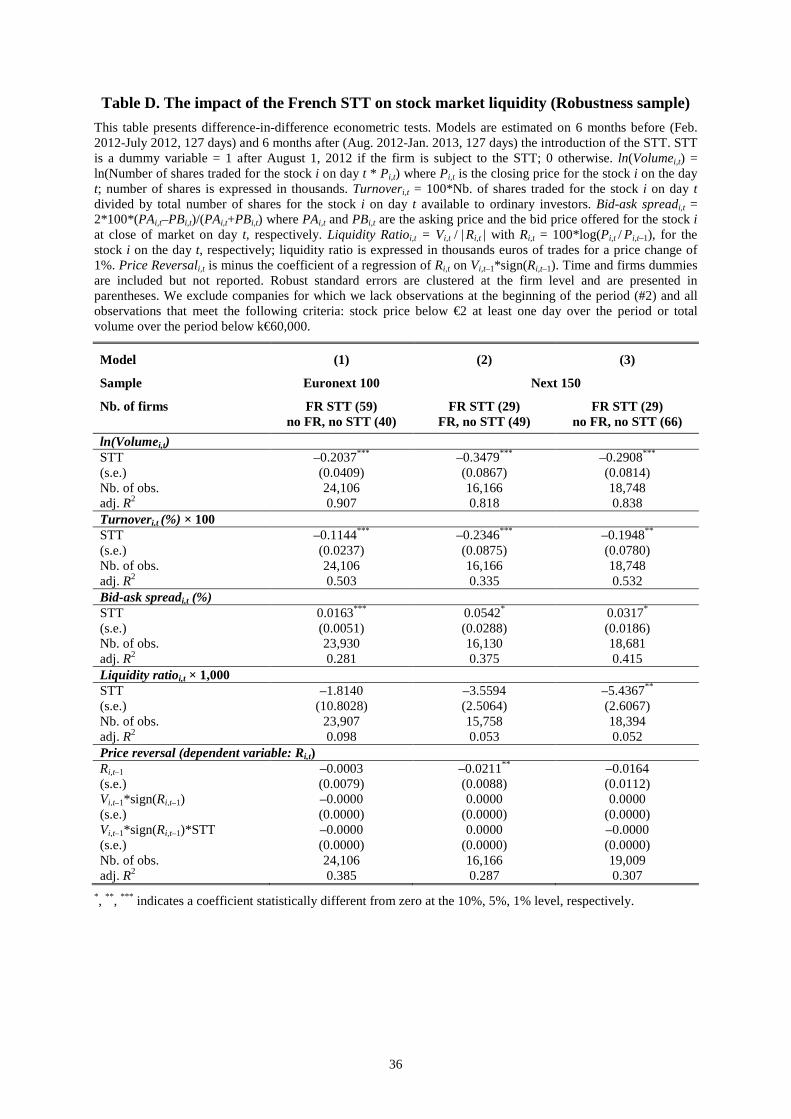
36

Table D. The impact of the French STT on stock market liquidity (Robustness sample)

This table presents difference-in-difference econometric tests. Models are estimated on 6 months before (Feb. 2012-July 2012, 127 days) and 6 months after (Aug. 2012-Jan. 2013, 127 days) the introduction of the STT. STT is a dummy variable = 1 after August 1, 2012 if the firm is subject to the STT; 0 otherwise. ln(Volumei,t) = ln(Number of shares traded for the stock i on day t * Pi,t) where Pi,t is the closing price for the stock i on the day t; number of shares is expressed in thousands. Turnoveri,t = 100*Nb. of shares traded for the stock i on day t divided by total number of shares for the stock i on day t available to ordinary investors. Bid-ask spreadi,t = 2*100*(PAi,t–PBi,t)/(PAi,t+PBi,t) where PAi,t and PBi,t are the asking price and the bid price offered for the stock i at close of market on day t, respectively. Liquidity Ratioi,t = Vi,t / |

Ri,t | with Ri,t = 100*log(Pi,t / Pi,t–1), for the

stock i on the day t, respectively; liquidity ratio is expressed in thousands euros of trades for a price change of 1%. Price Reversali,t is minus the coefficient of a regression of Ri,t on Vi,t–1*sign(Ri,t–1). Time and firms dummies are included but not reported. Robust standard errors are clustered at the firm level and are presented in parentheses. We exclude companies for which we lack observations at the beginning of the period (#2) and all observations that meet the following criteria: stock price below €2 at least one day over the period or total volume over the period below k€60,000.

Model (1) (2) (3)





ln(Volumei,t) STT –0.2037*** –0.3479*** –0.2908*** (s.e.) (0.0409) (0.0867) (0.0814) Nb. of obs. 24,106 16,166 18,748 adj. R2 0.907 0.818 0.838 Turnoveri,t (%) × 100 STT –0.1144*** –0.2346*** –0.1948** (s.e.) (0.0237) (0.0875) (0.0780) Nb. of obs. 24,106 16,166 18,748 adj. R2 0.503 0.335 0.532 Bid-ask spreadi,t (%) STT 0.0163*** 0.0542* 0.0317* (s.e.) (0.0051) (0.0288) (0.0186) Nb. of obs. 23,930 16,130 18,681 adj. R2 0.281 0.375 0.415 Liquidity ratioi,t × 1,000 STT –1.8140 –3.5594 –5.4367** (s.e.) (10.8028) (2.5064) (2.6067) Nb. of obs. 23,907 15,758 18,394 adj. R2 0.098 0.053 0.052 Price reversal (dependent variable: Ri,t) Ri,t–1 –0.0003 –0.0211** –0.0164 (s.e.) (0.0079) (0.0088) (0.0112) Vi,t–1*sign(Ri,t–1) –0.0000 0.0000 0.0000 (s.e.) (0.0000) (0.0000) (0.0000) Vi,t–1*sign(Ri,t–1)*STT –0.0000 0.0000 –0.0000 (s.e.) (0.0000) (0.0000) (0.0000) Nb. of obs. 24,106 16,166 19,009 adj. R2 0.385 0.287 0.307


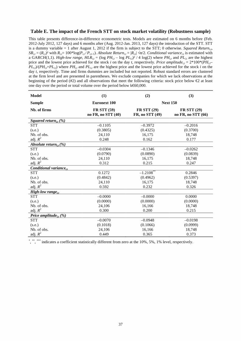
37

Table E. The impact of the French STT on stock market volatility (Robustness sample)

This table presents difference-in-difference econometric tests. Models are estimated on 6 months before (Feb. 2012-July 2012, 127 days) and 6 months after (Aug. 2012-Jan. 2013, 127 days) the introduction of the STT. STT is a dummy variable = 1 after August 1, 2012 if the firm is subject to the STT; 0 otherwise. Squared Returni,t, SRi,t = (Ri,t)² with Ri,t= 100*log(Pi,t / Pi,t–1). Absolute Returni,t = |Ri,t| √π/2. Conditional variancei,t is estimated with a GARCH(1,1). High-low range, HLRi,t = (log PHi,t – log PLi,t)² / 4 log(2) where PHi,t and PLi,t are the highest price and the lowest price achieved for the stock i on the day t, respectively. Price amplitudei,t = 2*100*(PHi,t–PLi,t)/(PHi,t+PLi,t) where PHi,t and PLi,t are the highest price and the lowest price achieved for the stock i on the day t, respectively. Time and firms dummies are included but not reported. Robust standard errors are clustered at the firm level and are presented in parentheses. We exclude companies for which we lack observations at the beginning of the period (#2) and all observations that meet the following criteria: stock price below €2 at least one day over the period or total volume over the period below k€60,000.

Model (1) (2) (3)





Squared returni,t (%) STT –0.1105 –0.3972 –0.2016 (s.e.) (0.3805) (0.4325) (0.3700) Nb. of obs. 24,110 16,175 18,748 adj. R2 0.248 0.162 0.177 Absolute returni,t (%) STT –0.0304 –0.1346 –0.0262 (s.e.) (0.0790) (0.0890) (0.0839) Nb. of obs. 24,110 16,175 18,748 adj. R2 0.312 0.215 0.247 Conditional variancei,t STT 0.1272 –1.2108** 0.2846 (s.e.) (0.4842) (0.4962) (0.5397) Nb. of obs. 24,110 16,175 18,748 adj. R2 0.592 0.232 0.326 High-low rangei,t STT –0.0000 –0.0000 0.0000 (s.e.) (0.0000) (0.0000) (0.0000) Nb. of obs. 24,106 16,166 18,748 adj. R2 0.300 0.200 0.215 Price amplitudei,t (%) STT –0.0070 –0.0948 –0.0198 (s.e.) (0.1018) (0.1066) (0.0999) Nb. of obs. 24,106 16,166 18,748 adj. R2 0.449 0.365 0.373


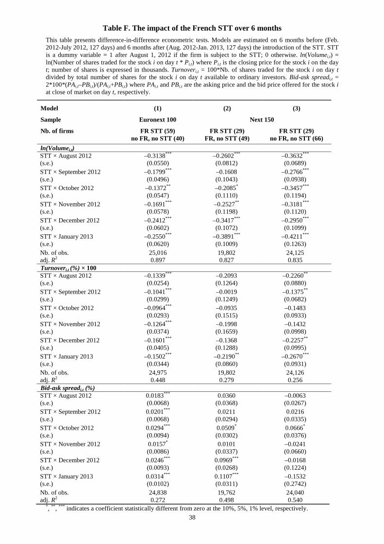
38

Table F. The impact of the French STT over 6 months

This table presents difference-in-difference econometric tests. Models are estimated on 6 months before (Feb. 2012-July 2012, 127 days) and 6 months after (Aug. 2012-Jan. 2013, 127 days) the introduction of the STT. STT is a dummy variable = 1 after August 1, 2012 if the firm is subject to the STT; 0 otherwise. ln(Volumei,t) = ln(Number of shares traded for the stock i on day t * Pi,t) where Pi,t is the closing price for the stock i on the day t; number of shares is expressed in thousands. Turnoveri,t = 100*Nb. of shares traded for the stock i on day t divided by total number of shares for the stock i on day t available to ordinary investors. Bid-ask spreadi,t = 2*100*(PAi,t–PBi,t)/(PAi,t+PBi,t) where PAi,t and PBi,t are the asking price and the bid price offered for the stock i at close of market on day t, respectively.

Model (1) (2) (3)





ln(Volumei,t) STT × August 2012 –0.3138*** –0.2602*** –0.3632*** (s.e.) (0.0550) (0.0812) (0.0689) STT × September 2012 –0.1799*** –0.1608 –0.2766*** (s.e.) (0.0496) (0.1043) (0.0938) STT × October 2012 –0.1372** –0.2085* –0.3457*** (s.e.) (0.0547) (0.1110) (0.1194) STT × November 2012 –0.1691*** –0.2527** –0.3181*** (s.e.) (0.0578) (0.1198) (0.1120) STT × December 2012 –0.2412*** –0.3417*** –0.2950*** (s.e.) (0.0602) (0.1072) (0.1099) STT × January 2013 –0.2550*** –0.3891*** –0.4211*** (s.e.) (0.0620) (0.1009) (0.1263) Nb. of obs. 25,016 19,802 24,125 adj. R2 0.897 0.827 0.835 Turnoveri,t (%) × 100 STT × August 2012 –0.1339*** –0.2093 –0.2260** (s.e.) (0.0254) (0.1264) (0.0880) STT × September 2012 –0.1041*** –0.0019 –0.1375** (s.e.) (0.0299) (0.1249) (0.0682) STT × October 2012 –0.0964*** –0.0935 –0.1483 (s.e.) (0.0293) (0.1515) (0.0933) STT × November 2012 –0.1264*** –0.1998 –0.1432 (s.e.) (0.0374) (0.1659) (0.0998) STT × December 2012 –0.1601*** –0.1368 –0.2257** (s.e.) (0.0405) (0.1288) (0.0995) STT × January 2013 –0.1502*** –0.2190** –0.2670*** (s.e.) (0.0344) (0.0860) (0.0931) Nb. of obs. 24,975 19,802 24,126 adj. R2 0.448 0.279 0.256 Bid-ask spreadi,t (%) STT × August 2012 0.0183*** 0.0360 –0.0063 (s.e.) (0.0068) (0.0368) (0.0267) STT × September 2012 0.0201*** 0.0211 0.0216 (s.e.) (0.0068) (0.0294) (0.0335) STT × October 2012 0.0294*** 0.0509* 0.0666* (s.e.) (0.0094) (0.0302) (0.0376) STT × November 2012 0.0157* 0.0101 –0.0241 (s.e.) (0.0086) (0.0337) (0.0660) STT × December 2012 0.0246*** 0.0969*** –0.0168 (s.e.) (0.0093) (0.0268) (0.1224) STT × January 2013 0.0314*** 0.1107*** –0.1532 (s.e.) (0.0102) (0.0311) (0.2742) Nb. of obs. 24,838 19,762 24,040 adj. R2 0.272 0.498 0.540


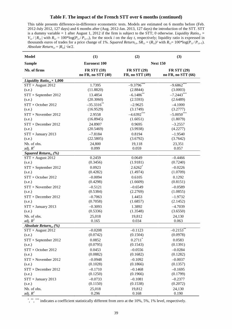
39

Table F. The impact of the French STT over 6 months (continued)

This table presents difference-in-difference econometric tests. Models are estimated on 6 months before (Feb. 2012-July 2012, 127 days) and 6 months after (Aug. 2012-Jan. 2013, 127 days) the introduction of the STT. STT is a dummy variable = 1 after August 1, 2012 if the firm is subject to the STT; 0 otherwise. Liquidity Ratioi,t = Vi,t / |

Ri,t | with Ri,t = 100*log(Pi,t / Pi,t–1), for the stock i on the day t, respectively; liquidity ratio is expressed in

thousands euros of trades for a price change of 1%. Squared Returni,t, SRi,t = (Ri,t)² with Ri,t= 100*log(Pi,t / Pi,t–1). Absolute Returni,t = |Ri,t| √π/2.

Model (1) (2) (3)





Liquidity Ratioi,t × 1,000 STT × August 2012 1.7395 –9.3796*** –9.6862*** (s.e.) (11.8820) (2.8844) (3.0003) STT × September 2012 13.4854 –6.1486** –7.2443*** (s.e.) (20.3060) (2.5593) (2.6489) STT × October 2012 –35.3316** –2.9625 –4.1000 (s.e.) (16.9529) (3.1749) (3.2777) STT × November 2012 2.9558 –4.6392*** –5.0050*** (s.e.) (16.8945) (1.6051) (1.8079) STT × December 2012 24.8907 0.9695 –3.2557 (s.e.) (20.5469) (3.9938) (4.2277) STT × January 2013 –7.8184 0.8194 –1.9540 (s.e.) (22.5805) (3.6792) (3.7642) Nb. of obs. 24,800 19,118 23,351 adj. R2 0.099 0.059 0.057 Squared Returni,t (%) STT × August 2012 0.2459 0.0649 –0.4466 (s.e.) (0.3456) (1.9181) (0.7240) STT × September 2012 0.0923 2.6262* –0.0226 (s.e.) (0.4282) (1.4974) (1.0709) STT × October 2012 –0.0094 0.6105 0.1292 (s.e.) (0.4298) (1.6609) (0.8151) STT × November 2012 –0.5121 –0.6549 –0.0589 (s.e.) (0.5384) (2.2769) (1.0855) STT × December 2012 –0.7063 1.4453 –1.9732 (s.e.) (0.7058) (1.6857) (2.1452) STT × January 2013 –0.3093 1.3892 –4.7039 (s.e.) (0.5336) (1.3548) (3.6550) Nb. of obs. 25,018 19,812 24,130 adj. R2 0.165 0.034 0.063 Absolute Returni,t (%) STT × August 2012 –0.0208 –0.1123 –0.2153** (s.e.) (0.0742) (0.1504) (0.0978) STT × September 2012 0.0852 0.2711* 0.0583 (s.e.) (0.0795) (0.1543) (0.1391) STT × October 2012 0.0453 –0.0556 –0.0284 (s.e.) (0.0882) (0.1682) (0.1282) STT × November 2012 –0.0948 –0.1092 –0.0037 (s.e.) (0.1028) (0.1866) (0.1357) STT × December 2012 –0.1710 –0.1468 –0.1695 (s.e.) (0.1250) (0.1966) (0.1799) STT × January 2013 –0.0733 –0.1081 –0.2377 (s.e.) (0.1150) (0.1538) (0.2072) Nb. of obs. 25,018 19,812 24,130 adj. R2 0.296 0.168 0.190


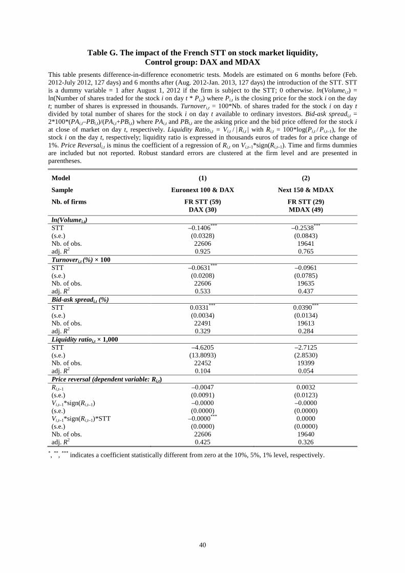
40

Table G. The impact of the French STT on stock market liquidity, Control group: DAX and MDAX

This table presents difference-in-difference econometric tests. Models are estimated on 6 months before (Feb. 2012-July 2012, 127 days) and 6 months after (Aug. 2012-Jan. 2013, 127 days) the introduction of the STT. STT is a dummy variable = 1 after August 1, 2012 if the firm is subject to the STT; 0 otherwise. ln(Volumei,t) = ln(Number of shares traded for the stock i on day t * Pi,t) where Pi,t is the closing price for the stock i on the day t; number of shares is expressed in thousands. Turnoveri,t = 100*Nb. of shares traded for the stock i on day t divided by total number of shares for the stock i on day t available to ordinary investors. Bid-ask spreadi,t = 2*100*(PAi,t–PBi,t)/(PAi,t+PBi,t) where PAi,t and PBi,t are the asking price and the bid price offered for the stock i at close of market on day t, respectively. Liquidity Ratioi,t = Vi,t / |

Ri,t | with Ri,t = 100*log(Pi,t / Pi,t–1), for the

stock i on the day t, respectively; liquidity ratio is expressed in thousands euros of trades for a price change of 1%. Price Reversali,t is minus the coefficient of a regression of Ri,t on Vi,t–1*sign(Ri,t–1). Time and firms dummies are included but not reported. Robust standard errors are clustered at the firm level and are presented in parentheses.

Model (1) (2)

Sample Euronext 100 & DAX Next 150 & MDAX

Nb. of firms FR STT (59) DAX (30)

FR STT (29) MDAX (49)

ln(Volumei,t) STT –0.1406*** –0.2538*** (s.e.) (0.0328) (0.0843) Nb. of obs. 22606 19641 adj. R2 0.925 0.765 Turnoveri,t (%) × 100 STT –0.0631*** –0.0961 (s.e.) (0.0208) (0.0785) Nb. of obs. 22606 19635 adj. R2 0.533 0.437 Bid-ask spreadi,t (%) STT 0.0331*** 0.0390*** (s.e.) (0.0034) (0.0134) Nb. of obs. 22491 19613 adj. R2 0.329 0.284 Liquidity ratioi,t × 1,000 STT –4.6205 –2.7125 (s.e.) (13.8093) (2.8530) Nb. of obs. 22452 19399 adj. R2 0.104 0.054 Price reversal (dependent variable: Ri,t) Ri,t–1 –0.0047 0.0032 (s.e.) (0.0091) (0.0123) Vi,t–1*sign(Ri,t–1) –0.0000 –0.0000 (s.e.) (0.0000) (0.0000) Vi,t–1*sign(Ri,t–1)*STT –0.0000*** 0.0000 (s.e.) (0.0000) (0.0000) Nb. of obs. 22606 19640 adj. R2 0.425 0.326


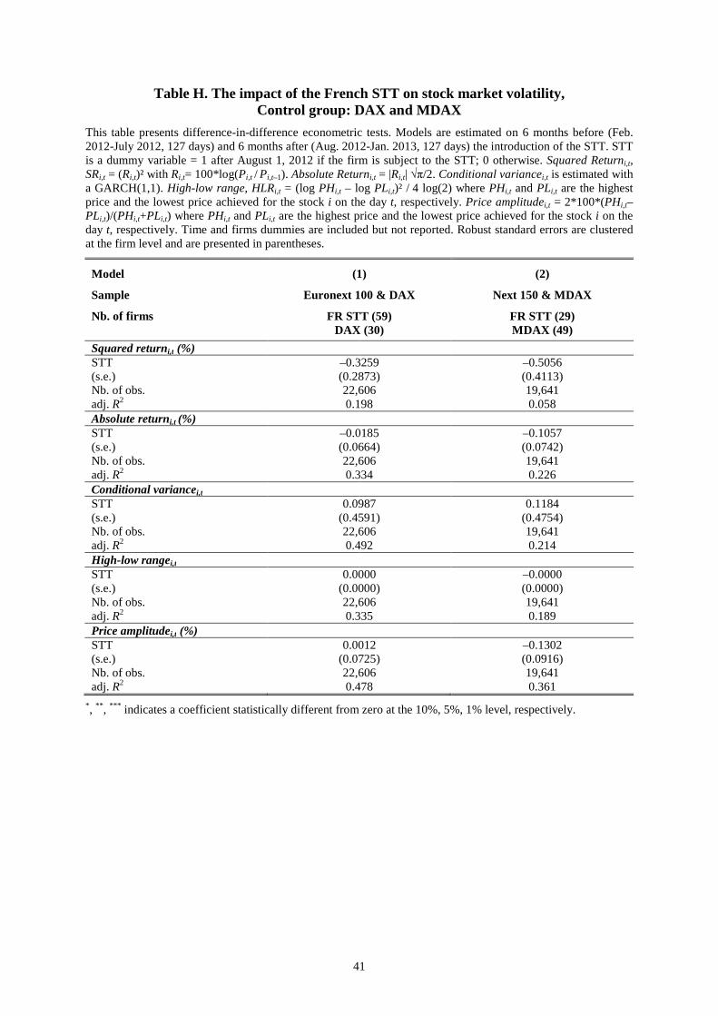
41

Table H. The impact of the French STT on stock market volatility, Control group: DAX and MDAX

This table presents difference-in-difference econometric tests. Models are estimated on 6 months before (Feb. 2012-July 2012, 127 days) and 6 months after (Aug. 2012-Jan. 2013, 127 days) the introduction of the STT. STT is a dummy variable = 1 after August 1, 2012 if the firm is subject to the STT; 0 otherwise. Squared Returni,t, SRi,t = (Ri,t)² with Ri,t= 100*log(Pi,t / Pi,t–1). Absolute Returni,t = |Ri,t| √π/2. Conditional variancei,t is estimated with a GARCH(1,1). High-low range, HLRi,t = (log PHi,t – log PLi,t)² / 4 log(2) where PHi,t and PLi,t are the highest price and the lowest price achieved for the stock i on the day t, respectively. Price amplitudei,t = 2*100*(PHi,t–PLi,t)/(PHi,t+PLi,t) where PHi,t and PLi,t are the highest price and the lowest price achieved for the stock i on the day t, respectively. Time and firms dummies are included but not reported. Robust standard errors are clustered at the firm level and are presented in parentheses.

Model (1) (2)

Sample Euronext 100 & DAX Next 150 & MDAX

Nb. of firms FR STT (59) DAX (30)

FR STT (29) MDAX (49)

Squared returni,t (%) STT –0.3259 –0.5056 (s.e.) (0.2873) (0.4113) Nb. of obs. 22,606 19,641 adj. R2 0.198 0.058 Absolute returni,t (%) STT –0.0185 –0.1057 (s.e.) (0.0664) (0.0742) Nb. of obs. 22,606 19,641 adj. R2 0.334 0.226 Conditional variancei,t STT 0.0987 0.1184 (s.e.) (0.4591) (0.4754) Nb. of obs. 22,606 19,641 adj. R2 0.492 0.214 High-low rangei,t STT 0.0000 –0.0000 (s.e.) (0.0000) (0.0000) Nb. of obs. 22,606 19,641 adj. R2 0.335 0.189 Price amplitudei,t (%) STT 0.0012 –0.1302 (s.e.) (0.0725) (0.0916) Nb. of obs. 22,606 19,641 adj. R2 0.478 0.361


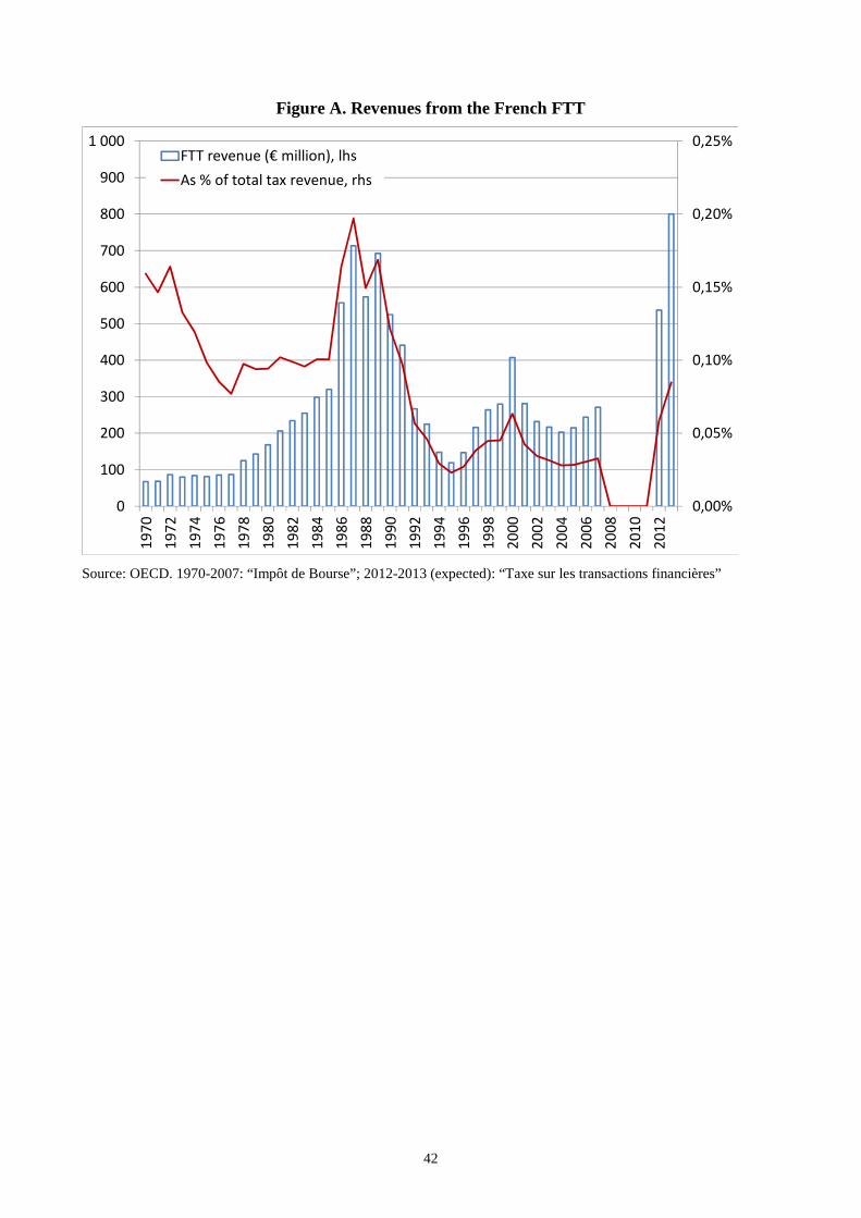
42

Figure A. Revenues from the French FTT

Source: OECD. 1970-2007: “Impôt de Bourse”; 2012-2013 (expected): “Taxe sur les transactions financières”

0,00%

0,05%

0,10%

0,15%

0,20%

0,25%

0

100

200

300

400

500

600

700

800

900

1 0001

97

0

19

72

19

74

19

76

19

78

19

80

19

82

19

84

19

86

19

88

19

90

19

92

19

94

19

96

19

98

20

00

20

02

20

04

20

06

20

08

20

10

20

12

FTT revenue (€ million), lhs

As % of total tax revenue, rhs

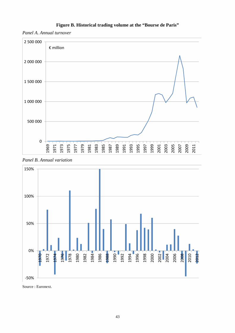
43

Figure B. Historical trading volume at the “Bourse de Paris”

Panel A. Annual turnover

Panel B. Annual variation

Source : Euronext.

0

500 000

1 000 000

1 500 000

2 000 000

2 500 000

19

69

19

71

19

73

19

75

19

77

19

79

19

81

19

83

19

85

19

87

19

89

19

91

19

93

19

95

19

97

19

99

20

01

20

03

20

05

20

07

20

09

20

11

€ million

-50%

0%

50%

100%

150%

19

70

19

72

19

74

19

76

19

78

19

80

19

82

19

84

19

86

19

88

19

90

19

92

19

94

19

96

19

98

20

00

20

02

20

04

20

06

20

08

20

10

20

12

The Impact of the French Securities Transaction Tax on ... · The Impact of the French Securities...

Documents

Transcript of The Impact of the French Securities Transaction Tax on ... · The Impact of the French Securities...