The Hurwitz Complex Continued Fraction

Doug Hensley

January 9, 2006

Abstract

The Hurwitz complex continued fraction algorithm generates Gaussianrational approximations to an arbitrary complex number α by way of asequence (a0, a1, . . .) of Gaussian integers determined by a0 = [α], z0 =α − a0, (where [u] denotes the Gaussian integer nearest u) and for j ≥ 1,aj = [1/zj−1], zj = 1/zj−1−aj . The rational approximations are the finitecontinued fractions [a0; a1, . . . , ar]. We establish a result for the Hurwitzalgorithm analogous to the Gauss-Kuz’min theorem, and we investigatea class of algebraic α of degree 4 for which the behavior of the resultingsequences 〈aj〉 and 〈zj〉 is quite different from that which prevails almosteverywhere.

1 Complex Continued Fractions

A complex continued fraction algorithm is, broadly speaking, an algorithm thatprovides approximations by ratios of Gaussian integers, or integers of anothercomplex number field, to a given complex number. We are faced with an immedi-ate choice: does speed matter, or does approximation quality trump everythingelse?

If quality of approximation is paramount, then the algorithm of choice is dueto Asmus Schmidt[7]. The basic idea is to partition (we ignore issues concerningbreaking ties at the boundaries) the complex plane into pieces bounded byline segments and arcs of circles, and to successively refine this partition. Thepartition component to which the target ξ belongs shrinks down to ξ as thisprocess is iterated.

Each component of the partition is associated with a linear fractional mapz → (az + b)/(cz + d), where the coefficients a, b, c, d are Gaussian integers, as

well as with the matrix

(a bc d

).

The Schmidt algorithm resembles the Lagarias multidimensional continuedfraction algorithm [5] in that both generate, for each ξ, a sequence 〈Mn(ξ)〉 ofmatrices with ‘integer’ entries, whose inverses also have ‘integer’ entries. Therequired Diophantine approximation to the target ξ can then be read off fromMn(ξ).

1

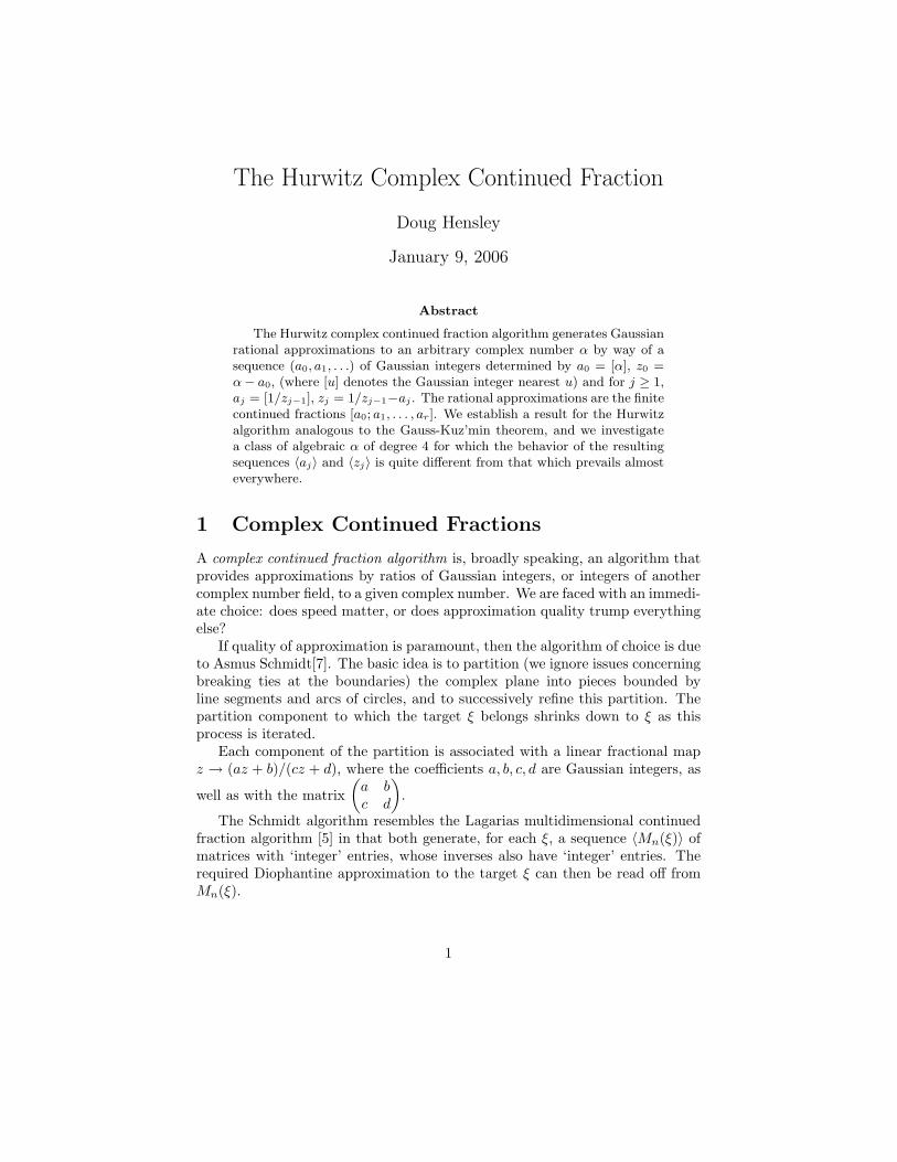
Figure 1: Fourth generation and (zoom to left-center) fifth.

It produces a tesselation of its space of possible targets, with the propertythat each set of ξ associated to a given Mn splits into some number of shards,each associated with a specific one of the possible successors MnT . We showthe fourth-generation partition of that portion of C bounded by the circle withdiameter (1, 1 + i):

On average, the Schmidt algorithm would appear to require only polyno-mial time in the binary length of the numerator and denominator of Gaussian-rational inputs. The worst-case is a different matter. Given a real input, or oneequivalent at an early stage to a real number, the algorithm can be quite slow.

2 The Hurwitz Complex Continued Fraction

If we relax the priority we set on quality of approximation, what do we get inexchange? Any complex continued fraction algorithm should take as input acomplex number z = z0, and return as output a sequence of approximations(pn/qn) to z, where pn, qn ∈ G = {a + ib : a ∈ Z, b ∈ Z} are relatively primeGaussian integers. The following properties are desirable:

1. The sequence (|qn|) increases at least exponentially.

2. The sequence (pn/qn) terminates in p/q if the input z is a Gaussian ratio-nal.

3. All approximations are of quality at least comparable to that which isknown to exist by virtue of the Dirichlet pigeonhole principle:

∣∣∣∣pn

qn− z

∣∣∣∣ ≪ |qn|−2

uniformly over n and over all inputs z.

2

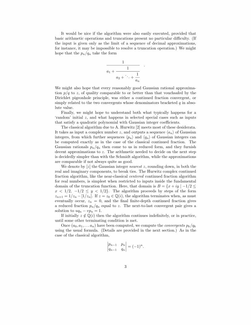
It would be nice if the algorithm were also easily executed, provided thatbasic arithmetic operations and truncations present no particular difficulty. (Ifthe input is given only as the limit of a sequence of decimal approximations,for instance, it may be impossible to resolve a truncation operation.) We mighthope that the pn/qn take the form

1

a1 +1

a2 +.. . +

1

an

.

We might also hope that every reasonably good Gaussian rational approxima-tion p/q to z, of quality comparable to or better than that vouchsafed by theDirichlet pigeonhole principle, was either a continued fraction convergent, orsimply related to the two convergents whose denominators bracketed q in abso-lute value.

Finally, we might hope to understand both what typically happens for a‘random’ initial z, and what happens in selected special cases such as inputsthat satisfy a quadratic polynomial with Gaussian integer coefficients.

The classical algorithm due to A. Hurwitz [2] meets most of these desiderata.It takes as input a complex number z, and outputs a sequence 〈an〉 of Gaussianintegers, from which further sequences 〈pn〉 and 〈qn〉 of Gaussian integers canbe computed exactly as in the case of the classical continued fraction. TheGaussian rationals pn/qn then come to us in reduced form, and they furnishdecent approximations to z. The arithmetic needed to decide on the next stepis decidedly simpler than with the Schmidt algorithm, while the approximationsare comparable if not always quite as good.

We denote by [z] the Gaussian integer nearest z, rounding down, in both thereal and imaginary components, to break ties. The Hurwitz complex continuedfraction algorithm, like the near-classical centered continued fraction algorithmfor real numbers, is simplest when restricted to inputs inside the fundamentaldomain of the truncation function. Here, that domain is B = {x + iy | −1/2 ≤x < 1/2, −1/2 ≤ y < 1/2}. The algorithm proceeds by steps of the formzn+1 = 1/zn − [1/zn]. If z = z0 ∈ Q(i), the algorithm terminates when, as musteventually occur, zn = 0, and the final finite-depth continued fraction givesa reduced fraction pn/qn equal to z. The next-to-last convergent pair gives asolution to uqn − vpn = 1.

If initially z /∈ Q(i) then the algorithm continues indefinitely, or in practice,until some other terminating condition is met.

Once (a0, a1, . . . an) have been computed, we compute the convergents pk/qk

using the usual formula. (Details are provided in the next section.) As in thecase of the classical algorithm,

∣∣∣∣pn−1 pn

qn−1 qn

∣∣∣∣ = (−1)n.

3

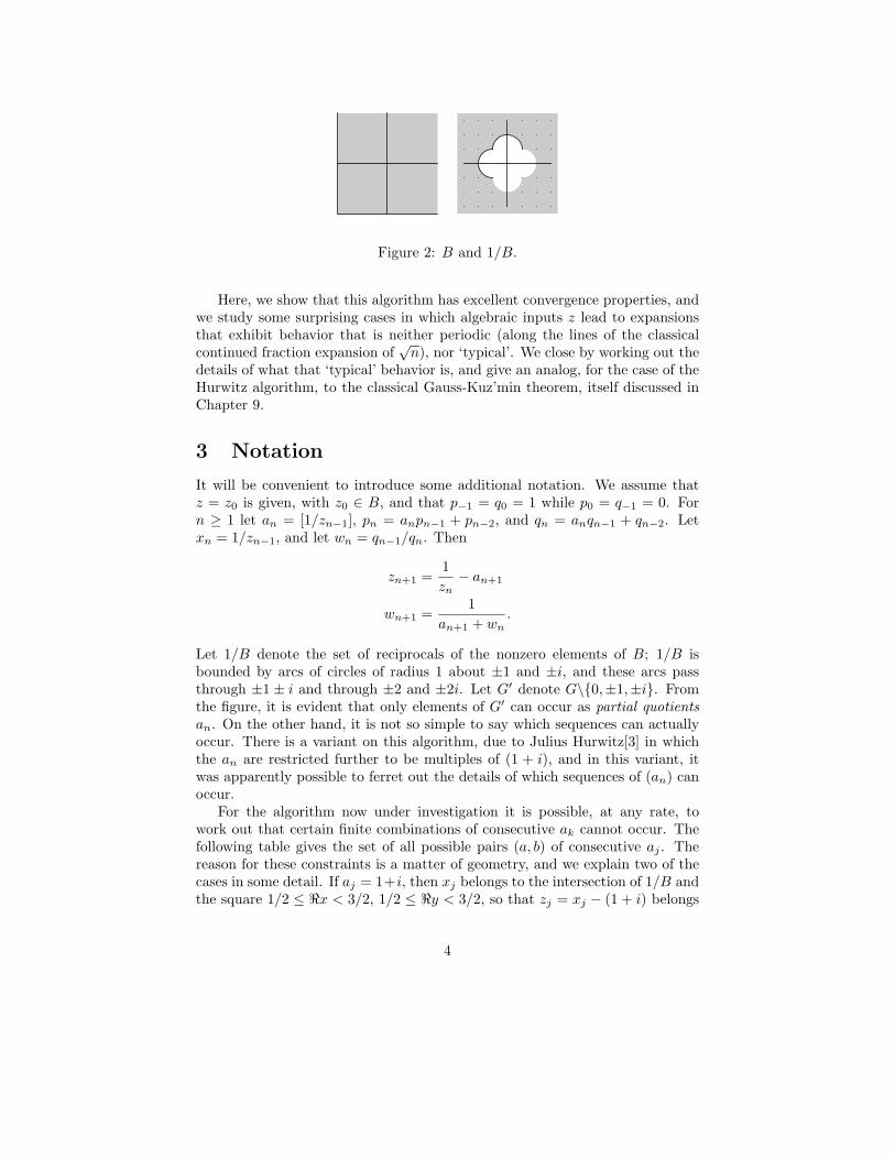
Figure 2: B and 1/B.

Here, we show that this algorithm has excellent convergence properties, andwe study some surprising cases in which algebraic inputs z lead to expansionsthat exhibit behavior that is neither periodic (along the lines of the classicalcontinued fraction expansion of

√n), nor ‘typical’. We close by working out the

details of what that ‘typical’ behavior is, and give an analog, for the case of theHurwitz algorithm, to the classical Gauss-Kuz’min theorem, itself discussed inChapter 9.

3 Notation

It will be convenient to introduce some additional notation. We assume thatz = z0 is given, with z0 ∈ B, and that p−1 = q0 = 1 while p0 = q−1 = 0. Forn ≥ 1 let an = [1/zn−1], pn = anpn−1 + pn−2, and qn = anqn−1 + qn−2. Letxn = 1/zn−1, and let wn = qn−1/qn. Then

zn+1 =1

zn− an+1

wn+1 =1

an+1 + wn.

Let 1/B denote the set of reciprocals of the nonzero elements of B; 1/B isbounded by arcs of circles of radius 1 about ±1 and ±i, and these arcs passthrough ±1 ± i and through ±2 and ±2i. Let G′ denote G\{0,±1,±i}. Fromthe figure, it is evident that only elements of G′ can occur as partial quotientsan. On the other hand, it is not so simple to say which sequences can actuallyoccur. There is a variant on this algorithm, due to Julius Hurwitz[3] in whichthe an are restricted further to be multiples of (1 + i), and in this variant, itwas apparently possible to ferret out the details of which sequences of (an) canoccur.

For the algorithm now under investigation it is possible, at any rate, towork out that certain finite combinations of consecutive ak cannot occur. Thefollowing table gives the set of all possible pairs (a, b) of consecutive aj . Thereason for these constraints is a matter of geometry, and we explain two of thecases in some detail. If aj = 1+i, then xj belongs to the intersection of 1/B andthe square 1/2 ≤ ℜx < 3/2, 1/2 ≤ ℜy < 3/2, so that zj = xj − (1 + i) belongs

4

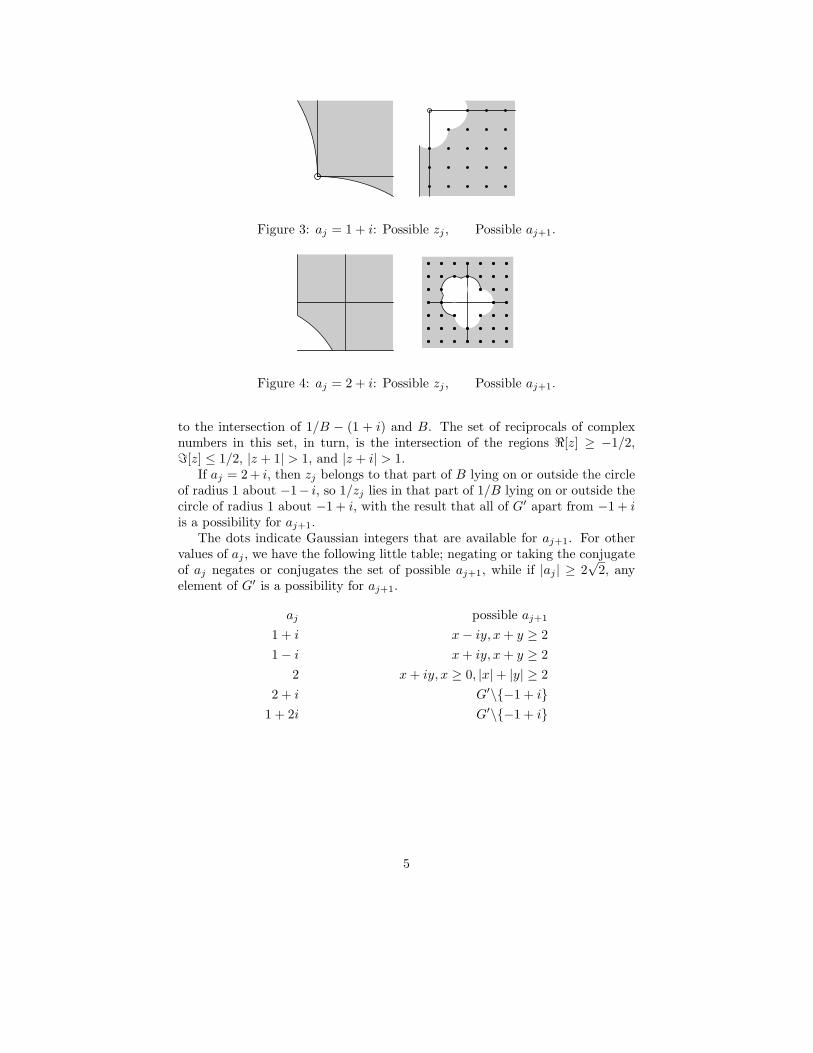
Figure 3: aj = 1 + i: Possible zj , Possible aj+1.

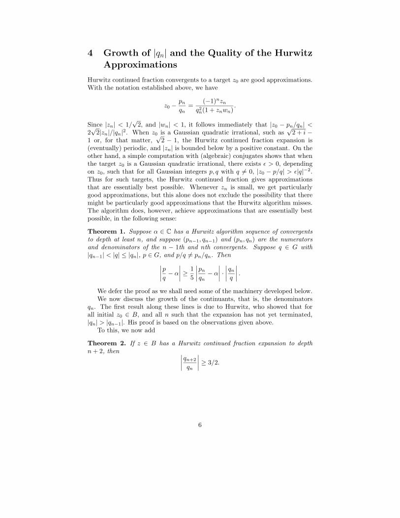
Figure 4: aj = 2 + i: Possible zj , Possible aj+1.

to the intersection of 1/B − (1 + i) and B. The set of reciprocals of complexnumbers in this set, in turn, is the intersection of the regions ℜ[z] ≥ −1/2,ℑ[z] ≤ 1/2, |z + 1| > 1, and |z + i| > 1.

If aj = 2 + i, then zj belongs to that part of B lying on or outside the circleof radius 1 about −1− i, so 1/zj lies in that part of 1/B lying on or outside thecircle of radius 1 about −1 + i, with the result that all of G′ apart from −1 + iis a possibility for aj+1.

The dots indicate Gaussian integers that are available for aj+1. For othervalues of aj , we have the following little table; negating or taking the conjugateof aj negates or conjugates the set of possible aj+1, while if |aj | ≥ 2

√2, any

element of G′ is a possibility for aj+1.

aj possible aj+1

1 + i x − iy, x + y ≥ 2

1 − i x + iy, x + y ≥ 2

2 x + iy, x ≥ 0, |x| + |y| ≥ 2

2 + i G′\{−1 + i}1 + 2i G′\{−1 + i}

5

4 Growth of |qn| and the Quality of the Hurwitz

Approximations

Hurwitz continued fraction convergents to a target z0 are good approximations.With the notation established above, we have

z0 −pn

qn=

(−1)nzn

q2n(1 + znwn)

.

Since |zn| < 1/√

2, and |wn| < 1, it follows immediately that |z0 − pn/qn| <2√

2|zn|/|qn|2. When z0 is a Gaussian quadratic irrational, such as√

2 + i −1 or, for that matter,

√2 − 1, the Hurwitz continued fraction expansion is

(eventually) periodic, and |zn| is bounded below by a positive constant. On theother hand, a simple computation with (algebraic) conjugates shows that whenthe target z0 is a Gaussian quadratic irrational, there exists ǫ > 0, dependingon z0, such that for all Gaussian integers p, q with q 6= 0, |z0 − p/q| > ǫ|q|−2.Thus for such targets, the Hurwitz continued fraction gives approximationsthat are essentially best possible. Whenever zn is small, we get particularlygood approximations, but this alone does not exclude the possibility that theremight be particularly good approximations that the Hurwitz algorithm misses.The algorithm does, however, achieve approximations that are essentially bestpossible, in the following sense:

Theorem 1. Suppose α ∈ C has a Hurwitz algorithm sequence of convergentsto depth at least n, and suppose (pn−1, qn−1) and (pn, qn) are the numeratorsand denominators of the n − 1th and nth convergents. Suppose q ∈ G with|qn−1| < |q| ≤ |qn|, p ∈ G, and p/q 6= pn/qn. Then

∣∣∣∣p

q− α

∣∣∣∣ ≥1

5

∣∣∣∣pn

qn− α

∣∣∣∣ ·∣∣∣∣qn

q

∣∣∣∣ .

We defer the proof as we shall need some of the machinery developed below.We now discuss the growth of the continuants, that is, the denominators

qn. The first result along these lines is due to Hurwitz, who showed that forall initial z0 ∈ B, and all n such that the expansion has not yet terminated,|qn| > |qn−1|. His proof is based on the observations given above.

To this, we now add

Theorem 2. If z ∈ B has a Hurwitz continued fraction expansion to depthn + 2, then ∣∣∣∣

qn+2

qn

∣∣∣∣ ≥ 3/2.

6

Proof. Recall that

qn+1 = an+1qn + qn−1

zn+1 =1

zn− an+1

wn+1 =1

an+1 + wn

an+1 =

[1

zn

]

qn

qn+1= wn+1.

Let Ga denote the set of possible values in G′ for the successor aj+1 to aj ifaj = a. We shall need some estimates for wn.

Lemma 1. Suppose z ∈ B, n ≥ 1, and z has a Hurwitz continued fraction todepth n + 2. If |wn| ≥ 2/3, then |wn+1| < 2/3. Furthermore, either |wn| < 2/3,or 2

3 ≤ |wn| < 1 and one of the following, or its negative or complex-conjugatecounterpart, holds:

∣∣∣∣wn − 9

14(1 − i)

∣∣∣∣ <3

7and an = 1 + i

∣∣∣∣wn − 9

16

∣∣∣∣ <3

16and an = 2.

The proof of the lemma is inductive and begins with the observation thatthe claim is true at the outset because w0 = 0. We use a fact about reciprocalsof disks: If D is a disk in C with center z and radius r, and if |z| > r, then withthe notation D(s, r) := {z ∈ C : |z − s| < r},

1

D(s, r)= D

(s

|s|2 − r2,

r

|s|2 − r2

).

Now let D0 be the disk about 0 with radius 2/3, and let D1 = 1/(1 + i +D0) = D((9/14)(1 − i), 3/7), D2 = 1/(−1 + i + D0), D3 = −1/(1 + i + D0),D4 = 1/(1−i+D0), D5 = 1/(2+D0), D6 = 1/(2i+D0), D7 = −1/(2+D0), andD8 = 1/(−2i + D0). Assuming the claim to be true for k ≤ n, we have eitherthat |wn| ∈ D0, or that wn lies in the intersection of one of 8 other disks withthe open unit disk, and an takes a corresponding specific value, either ±1± i or±2 or ±2i.

Now if |a| ≥√

5, then 1/(a + D0) ⊆ D0, while if a is one of the 8 Gaussianintegers in G′ nearest the origin, 1/(a + D0) is one of D1, . . . ,D8. Thus theinductive step cannot fail in the case that wn ∈ D0. On the other hand, for1 ≤ k ≤ 8, one readily checks that for any eligible successor a to an, 1/(Dk+a) ⊆D0. Thus, for instance, when wn ∈ D1\D0, we have an = 1 + i so that an+1 ∈G1+i = {u − iv : u ≥ 0, v ≥ 0, u + v ≥ 2}. For a ∈ G1+i, though, if |a| ≥ 2

√2

and |w| < 1 then |1/(a+w)| < 2/3, while if a ∈ {2, 2− i, 1− i, 1−2i,−2i} then,

7

from case by case calculation, 1/(a + D1) ⊂ D0. For instance, 1/(1− i + D1) =D((23/73)(1+i), 6/73), while 1/(2−i+D1) = D(37/133+23i/133, 6/133). Thusthe inductive step cannot fail in any of these other cases either, as |wn+1| < 2/3.We now note that we have shown that whenever |wn| ≥ 2/3, |wn+1| < 2/3.

At this point the proof of the theorem falls right out: |wn||wn+1| < 2/3because both factors are less than 1 and one of them is less than 2/3, and so|qn+2/qn| = 1/|wnwn+1| > 3/2.

We now give the proof of theorem 1. We first write (p, q) = s(pn−1, qn−1) +t(pn, qn). If s = 0 the estimate is immediate. We now break the question intotwo main cases: |s| = 1 and |s| > 1.

If |s| = 1, then we may multiply s and t by the same unit and so take s = 1.Now |α − pn/qn| = |zn|/(|qn(qn + znqn−1)|). Thus we must show that if q 6= qn

then ∣∣∣∣pn + znpn−1

qn + znqn−1− tpn + pn−1

tqn + qn−1

∣∣∣∣ >1

5

|zn||q(qn + znqn−1)|

,

or equivalently, |t − 1/zn| > 1/5. Now q = qn+1 if and only if t = [1/zn]. But|q| ≤ |qn| < |qn+1|, so t 6= [1/zn], so |t − 1/zn| ≥ 1/2. This completes the prooffor the case |s| = 1.

We break the case |s| > 1 down into subcases depending on the value of an.There is sufficient symmetry that rotations and reflections are of no consequence,so these cases reduce to the following: |an| ≥ 3, an = 2 + 2i, an = 2 + i, an = 2,and an = 1 + i. We now assume that p/q gives a counterexample at depth n.The premise |qn−1| < |q| ≤ |qn| gives |wn| < |swn +t| ≤ 1, while our assumptionthat p/q is a good approximation to α gives |s/zn − t| ≤ (1/5). Equivalently,

∣∣∣∣1

zn− t

s

∣∣∣∣ ≤1

5|s| ,∣∣∣∣wn +

t

s

∣∣∣∣ ≤1

|s| .

From these it follows that |wn + 1/zn| < 6/5|s|).Now the value of an constrains both wn and zn. It constrains wn because

wn = 1/(an+wn−1) and |wn−1| < 1. Thus, wn belongs to the disk D(an/(|an|2−1), 1/(|an|2−1)) where D(c, r) denotes the disk {z ∈ C : |z− c| < r}. The effectof an upon the possible values of zn comes from the fact that zn ∈ D(an, 1)∩B,which becomes important only when |an| ≤

√5.

For the case |an| ≥ 3, we have |wn| < 1/2 while |1/zn| ≥√

2, so |wn+1/zn| >√2 − 1/2 > 6/5

√2. If an = 2 + 2i then wn ∈ D((2 − 2i)/7, 1/7). Thus

it will suffice to complete this case, that D((−2 + 2i)/7, (1/7 + 6/(5√

2)) sitsinside the union of the disks about ±1 and ±i of radius 1. It does, since| − (1 + i) + (2 − 2i)/7| = 5

√2/7 > 6/(5

√2) + 1/7.

If an = 2 + i then zn ⊆ B\D(−1 − i, 1), so 1/zn lies outside the union ofthe disks of radius 1 about ±1, ±i, and −1 + i. On the other hand, wn ∈D((2 − i)/4, 1/4)). The disk about −(2 − i)/4 of radius (1/4 + 6/(5

√2)) fits

comfortably within the region from which 1/zn is excluded, which completesthe proof for the case an = 2 + i.

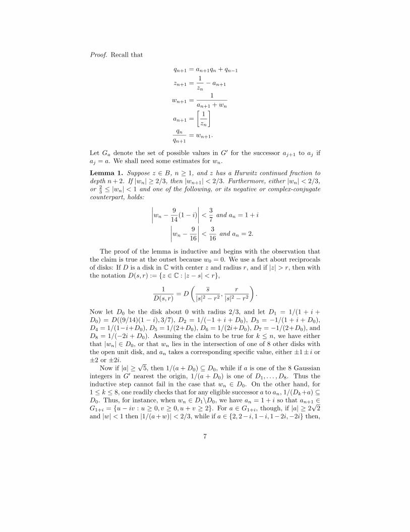
If an = 2, then wn ∈ D(2/3, 1/3) while zn ∈ B\D(−1, 1) so that 1/zn

belongs outside the union of our disks and the half-space ℜz < −1/2. The disk

8

Figure 5: Excluded values of 1/zn and disks for −wn.

D(−2/3, 1/3 + 6/(5√

2)) fits comfortably inside the region from which 1/zn isexcluded, which completes the proof for the case an = 2.

Finally, if an = 1 + i, then wn ∈ D(1 − i, 1) while zn ∈ B\(D(−1, 1) ∪D(−i, 1)). Thus 1/zn is excluded from the union of our four unit disks about±1 and ±i, and the half-planes ℜz < −1/2 and ℑz > 1/2. But D(−1 + i, 1 +6/(5

√2)) fits comfortably within this excluded zone.

5 Distribution of the Remainders

The sequence 〈zn〉 of remainders arising out of execution of the Hurwitz con-tinued fraction algorithm on input z0 depends, of course, on the input z0. If z0

is rational, then it terminates. If z0 is a Gaussian quadratic irrational, that is,if z0 satisfies a quadratic polynomial over Q(i), then it is ultimately periodic.[2]. These things are no surprise in view of what is known about the classicalcontinued fraction algorithm.

In the classical theory of continued fractions, we have the famous Gauss-Kuz’min theorem to the effect that if X is taken at random with uniformdistribution in [0, 1], then the probability density function of T kX convergesexponentially fast to the Gauss density 1

log 21

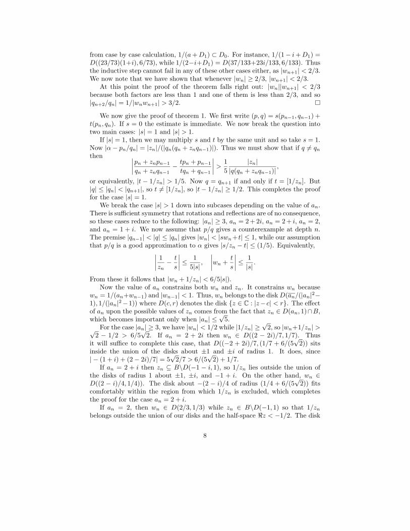
1+x on [0, 1]. This density is char-acterized by the fact that it is absolutely continuous with respect to Lebesguemeasure and is invariant under the map x → 1/x − ⌊1/x⌋. Numerical experi-ments suggest that something in the same vein might be true for the Hurwitzcomplex continued fraction. We do obtain such a theorem, but for the mo-ment, we just show a picture of the density that plays the role for the Hurwitzcontinued fraction that the Gauss density plays for the classical real continuedfraction.

The invariant density ρ for the Hurwitz algorithm is, in its own way, ratherpretty: we show here a false-color image of a somewhat crudely computed ap-proximation to it. A simple expression for this invariant density is not known,but the topic is new and there may well be one. The figure suggests, and welater prove, that this density is real-analytic on the interiors of the 12 regionsinto which arcs of circles of radius 1 centered at ±1, ±i, and ±1± i cut B, andthat it has the symmetry group of the rotations and reflections that map B toitself. A key fact is that T maps the union of these arcs, and the boundary ofB, into that same union.

Knowing this density, we can determine the relative frequency of the partialquotients aj . For instance, the limiting frequency with which aj = (1 + i), as

9

Figure 6: Invariant density for the Hurwitz algorithm.

j → ∞, is∫

E[1+i]ρ, where E[a] = {z ∈ B : [1/z] = a}, so that E[1 + i] is the

region bounded by the line segments 1/2+it,−1/2 ≤ t ≤ −√

3/6, t−i/2,√

3/6 ≤t ≤ 1/2, and by arcs of the circles |z − 1/3| = 1/3 and |z + i/3| = 1/3 joining(1 − i)/3 and (1 − i)/2. We can also make a well-founded conjecture as tothe average speed with which the algorithm brings a random Gaussian-rationalinput to zero.

As in the case of the rational integers and the classical gcd algorithm, a con-tinued fraction algorithm executed on rational inputs is, en passant, computingthe gcd of the input pair, as well as auxiliary information. Consider an inputz0 = s0/t0. As execution of the Hurwitz algorithm proceeds, successive zn =sn/tn are computed according to the rule zn+1 = 1/zn − [1/zn] = 1/zn − an+1.From this, we have sn+1tn+1 = sntn(1 − an+1zn) = sntnzn+1zn. We conjec-ture that for typical random rational inputs drawn from |s0| < R, |t0| < Rsay, the distribution of (zn) more or less conforms to ρ, except at the begin-ning, where it will be more uniform, or near the end when it will of necessitybe concentrated on a few simple Gaussian rationals. From this it would followthat the average number of steps needed to execute the Gaussian gcd algorithmshould be proportional to log |tn|, with the constant of proportionality being1/

∫B

log |z|ρ(z) dm(z). This integral was estimated by Monte Carlo methods tobe 1.092766. Numerical tests of the conjecture on 100 pseudorandom pairs withs, t chosen at random among Gaussian integers with real and imaginary partsof absolute value less than 101000 gave an aggregate of 210863 steps to finish all100 inputs, as against a predicted value of 210679.

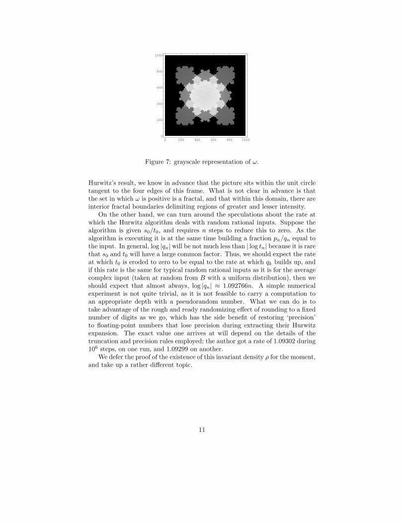
It would be nice to know the asymptotic behavior of the growth of qn. Forthis, it would seem at first that we would need the distribution of wn; if wehad a function ω along the lines of ρ for the distribution of the successive wn,n

∫D

(− log |z|ω(z)) would be the expected value of log |qn|. This hypothetical ωcan be guessed at by amassing some statistics; here is a pictures of the result.The range of the picture is the square |ℜ(z)| ≤ 1, |ℑ(z)| ≤ 1. On grounds of

10

0 200 400 600 800 10000

200

400

600

800

1000

Figure 7: grayscale representation of ω.

Hurwitz’s result, we know in advance that the picture sits within the unit circletangent to the four edges of this frame. What is not clear in advance is thatthe set in which ω is positive is a fractal, and that within this domain, there areinterior fractal boundaries delimiting regions of greater and lesser intensity.

On the other hand, we can turn around the speculations about the rate atwhich the Hurwitz algorithm deals with random rational inputs. Suppose thealgorithm is given s0/t0, and requires n steps to reduce this to zero. As thealgorithm is executing it is at the same time building a fraction pn/qn equal tothe input. In general, log |qn| will be not much less than | log tn| because it is rarethat s0 and t0 will have a large common factor. Thus, we should expect the rateat which t0 is eroded to zero to be equal to the rate at which qk builds up, andif this rate is the same for typical random rational inputs as it is for the averagecomplex input (taken at random from B with a uniform distribution), then weshould expect that almost always, log |qn| ≈ 1.092766n. A simple numericalexperiment is not quite trivial, as it is not feasible to carry a computation toan appropriate depth with a pseudorandom number. What we can do is totake advantage of the rough and ready randomizing effect of rounding to a fixednumber of digits as we go, which has the side benefit of restoring ‘precision’to floating-point numbers that lose precision during extracting their Hurwitzexpansion. The exact value one arrives at will depend on the details of thetruncation and precision rules employed; the author got a rate of 1.09302 during106 steps, on one run, and 1.09299 on another.

We defer the proof of the existence of this invariant density ρ for the moment,and take up a rather different topic.

11

6 A Class of Algebraic Approximants with Atyp-

ical Hurwitz Continued Fraction Expansions

Algebraic numbers may be expected to perhaps have atypical diophantine ap-proximation properties. When we are dealing with real numbers, the situationis not all that well understood but certain things are well-known. Rationalnumbers have terminating continued fraction expansions. Real roots α of an ir-reducible quadratic polynomial over Q have ultimately periodic continued frac-tion expansions. As a result of this, the sequence of remainders is ultimatelyperiodic, while the sequence of scaled errors q2

n(α − pn/qn) converges to a pe-riodic loop. For real α of degree greater than 2, there are results concerningsimultaneous diophantine approximation of the powers of α, but concerningα alone, all we know is that the continued fraction expansion cannot involveextraordinarily large integers, such as would be typical of Liouville numbers.Thus, the theoretical frequency of 1, 2, . . . , 10 according to the Gauss densityis (0.415037, 0.169925, 0.0931094, 0.0588937, 0.040642, 0.0297473, 0.0227201,0.0179219, 0.0144996, 0.0119726), while the actual frequency of these same par-tial quotients in the expansion of 21/3 to a depth of 10000 is (0.4173, 0.1675,0.0946, 0.0636, 0.0421, 0.0295, 0.024, 0.0163, 0.0122, 0.0118).

In the case of the Hurwitz algorithm, at first it seems that we are in for moreof the same. When the approximation target is in Q(i), the algorithm termi-nates, having found a reduced Gaussian rational equal to the original target.When the approximation target satisfies an irreducible quadratic polynomialover Q(i), the Hurwitz expansion is ultimately periodic. [2]. But if we looka bit further, we come upon a new behavior. Somewhat typical here is whathappens with z0 =

√2 − 1 + i(

√5 − 2). This z0 satisfies an irreducible quartic

polynomial over Q(i), to wit, x4+(4+8i)x3−(12−24i)x2−(32−16i)x+24. Butthe Hurwitz continued fraction expansion of z0 is neither ultimately periodic,nor anything like the typical expansion. Instead, what we see is that

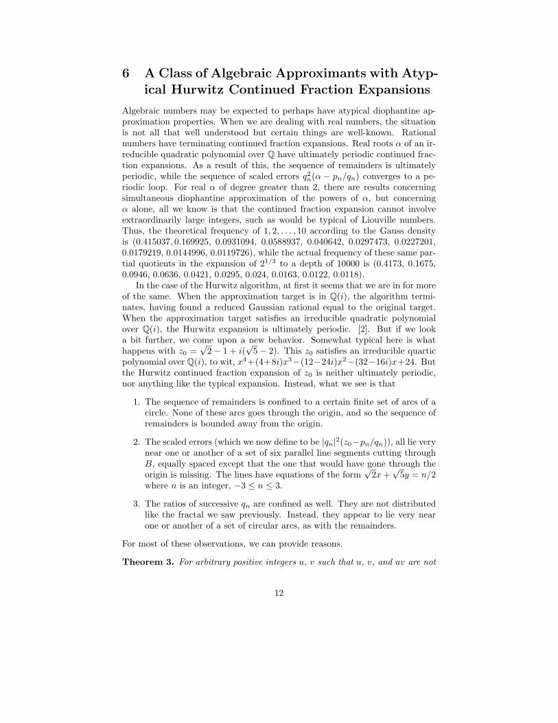
1. The sequence of remainders is confined to a certain finite set of arcs of acircle. None of these arcs goes through the origin, and so the sequence ofremainders is bounded away from the origin.

2. The scaled errors (which we now define to be |qn|2(z0−pn/qn)), all lie verynear one or another of a set of six parallel line segments cutting throughB, equally spaced except that the one that would have gone through theorigin is missing. The lines have equations of the form

√2x +

√5y = n/2

where n is an integer, −3 ≤ n ≤ 3.

3. The ratios of successive qn are confined as well. They are not distributedlike the fractal we saw previously. Instead, they appear to lie very nearone or another of a set of circular arcs, as with the remainders.

For most of these observations, we can provide reasons.

Theorem 3. For arbitrary positive integers u, v such that u, v, and uv are not

12

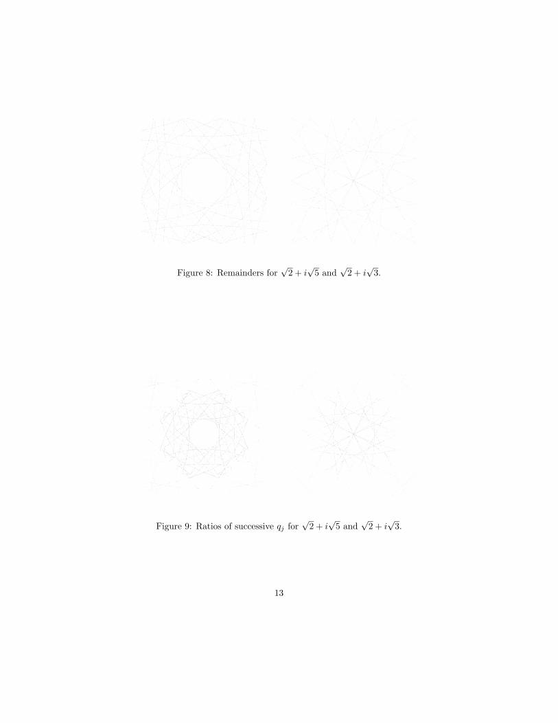
Figure 8: Remainders for√

2 + i√

5 and√

2 + i√

3.

Figure 9: Ratios of successive qj for√

2 + i√

5 and√

2 + i√

3.

13

square, there is a finite set A of circles and lines in C such that for all j ≥ 1,T jz0 ∈ ∪A∈AA ∩ B.

Proof. Let C(γ, r) denote the circle in C about γ of radius r. Fix positiveintegers u and v, neither square, and assume that uv is also not square. Let a0 =[√

u + i√

v], and let z0 =√

u + i√

v − a0 ∈ B. As z0 is not a Gaussian rational,the Hurwitz continued fraction expansion of z0 is infinite. Let 〈z0, z1, . . .〉 bethe sequence of remainders, and 〈a0, a1, . . .〉 the sequence of partial quotients,thus generated. Let 〈p0, p1, . . .〉 and 〈q0, q1, . . .〉 the sequence of numerators anddenominators, generated by the Hurwitz algorithm on input

√u + i

√v. By

convention, p−1 = 1, q−1 = 0, p0 = a0, and q0 = 1. Let w0 = 0, and for j ≥ 1,let wj = qj−1/qj . Equivalently, for j ≥ 1, wj = 1/(aj + wj−1).

We now consider a variant of the Hurwitz algorithm in which we keep tracknot only of the points zn = Tnz0, but of particular circles or lines on which zn

must lie. Our variant algorithm starts at an initial state (z0, C(−a0,√

m). Allstates have the form (x,K), where K is either a circle passing through B of theform (C(γ/d,

√m/|d|)) with γ ∈ G∗, d ∈ Z∗, and d | (|γ|2−m), and with radius

r =√

m/|d| satisfying 1/(2√

2) ≤ r ≤ √m, or a line passing through B of the

form L(k/(2δ), iδ) where k ∈ Z and |δ|2 = m.Let T (x,K) = (1/x − a, φa(K)) where a = [1/x] and φa is the linear frac-

tional map given by φa(z) = 1/z − a.Each statement below is readily verified and the details are left to the reader.

1. If x ∈ K ∩ B, K is a circle of the form C(γ/d,√

m/|d|) with d ∈ Z∗, d |(|γ|2 − m) 6= 0, and

√m/d ≥ 1/(2

√2), then T (x,K) = (x′,K ′) where

x′ ∈ K ′ ∩B and K ′ is another circle of the same form satisfying the sameconditions.

2. If x ∈ K∩B, K is a circle of the form C(γ/d,√

m/d) with d ∈ Z∗, |γ|2 = m,and

√m/d ≥ 1/(2

√2), then T (x,K) = (x′,K ′) with x′ ∈ B ∩K ′, and K ′

is the line L((d − 2ℜ(aγ))/(2γ), iγ), which passes through B.

3. If x ∈ K ∩ B and K is a line of the form L(0, iδ) with |δ|2 = m, thenT (x,K) = (x′,K ′) where K ′ = L(−ℜ(aδ)/δ, iδ).

4. If x ∈ K∩B and K is a line of the form L(k/2δ, iδ) with k ∈ Z∗, and |δ|2 =

m then T (x,K) = (x′,K ′) where x′ ∈ K ′ ∩ B and K ′ = C(

δ−akk , |δ|

|k|

),

the new circle passes through 0 so that it has the required form, and theradius |δ|/|k| =

√m/|k| is at least 1/

√2 because the diameter of K ′ is at

least√

2 because it is the reciprocal of the distance from 0 to the pointon K nearest 0, and that nearest point lies within B and thus lies at adistance of less than 1/

√2 from 0.

There are only finitely many lines of the form L(k/2δ, iδ) passing through B,with |δ|2 = m. There are only finitely many circles of the form C(γ/d,

√m/|d|)

with γ ∈ G, d ∈ Z∗, d | (|γ|2 −m) 6= 0, and√

m/d ≥ 1/(2√

2). We take A to bethe set of all such lines and circles.

14

We now turn to the topic of scaled errors. Let ej be the scaled error for the

jth convergent. Since z0 = (pj + znpj−1)/(qj + znqj−1), and since

∣∣∣∣pj−1 pj

qj−1 qj

∣∣∣∣ =

(−1)j , the scaled errors are also given by

ej =(−1)jqjzj

qj + zjqj−1.

Theorem 4. Let u and v be positive integers. Let α =√

u + i√

v. Let p, q beGaussian integers with |q|2 ≥ 9, and assume |p − qα| ≤ 2

√2/|q|. Let e(q, p, α)

be the scaled error e(q, p, α) = q(qα − p). Then

ℜ(αe(q, p, α)) =n

2+ δ

where n = (|p|2 − (u + v)|q|2) is an integer satisfying |n| ≤ 8√

u + v and δ ∈ C

with |δ| ≤ 4/|q|2.Remark 1. In other words, the scaled errors lie almost, but not quite, on afinite set of parallel lines. The amount by which the scaled errors stand off fromthese lines is itself at most comparable to |q|−2.

Proof. Let p = p1 + ip2, q = q1 + iq2 with p1, p2, q1, q2 ∈ Z. Let c = p1q1 + p2q2,d = p2q1 − p1q2, so that c2 + d2 = |p|2|q|2. Let θ1 + iθ2 = e(q, p, α). Then thegiven conditions are then equivalent to

(p1 + ip2)(q1 − iq2) = |q|2(√u + i√

v) + θ1 + iθ2,

e(q, p, α) = (c − |q|2√u) + i(d − |q|2√v) = θ1 + iθ2,

θ21 + θ2

2 ≤ 8.

Thus, αe(q, p, α) = (θ1√

u + θ2√

v) + i(θ2√

u − θ1√

v), and

ℜ(αe(q, p, α)) = θ1

√u + θ2

√v = (c

√u − |q|2u) + (d

√v − |q|2v).

Turning this around, we have c = |q|2√u + θ1, d = |q|2√v + θ2, and so

|p|2|q|2 = c2 + d2 = |q|4(u + v) + 2|q|2(θ1

√u + θ2

√v) + (θ2

1 + θ22).

Hence,

(θ1

√u + θ2

√v) =

1

2(|p|2 − (u + v)|q|2) − θ2

1 + θ22

2|q|2 .

With n = |p|2 − (u + v)|q|2, we note that

|n| ≤ |p2 − (√

u + i√

v)2q2| = |p − αq||2αq + (p − αq)|

≤ 2√

2

|q|

(2√

u + v|q| + 2√

2

|q|

)≤ (4

√2√

u + v + 8/|q|2) ≤ 8√

u + v.

This takes us back to the question of just what is typical of the orbits Tnz?

15

7 The Gauss-Kuz’min Density for the Hurwitz

Algorithm

There can be more than one measure on a set that is invariant under a self-mapping T . There can, in principle, be more than one that is absolutely con-tinuous with respect to Lebesgue measure.

We are certainly not exempt from the first possibility, as there are periodicorbits and uniformly weighted discrete measures on these are invariant underT . But the second pathology does not exist.

Theorem 5. There is a unique measure µ on B that is absolutely continuouswith respect to Lebesgue measure and invariant under T . This measure hasa density function ρ; the density is continuous except perhaps along the arcs|z ± 1| = 1, |z ± i| = 1, and |z ± 1± i| = 1. It is real-analytic on an each of the12 open regions into which B◦ is dissected by these arcs. The mapping T on Bis mixing with respect to µ: for Lebesgue-measurable A1, A2 ⊆ B,

limn→∞

µ(T−nA1 ∩ A2) = µ(A1)µ(A2).

The expected symmetry obtains: µ(iA) = µ(A) and µ(A) = µ(A) for all mea-surable A.

The general plan of the proof is this: We show that if f is a continuousprobability density function on B and X a random variable on B with densityf , then there exists a positive integer n, depending on f , and ǫ > 0, such thatthe density of TnX is greater than ǫ everywhere in B◦.

The theory of positive operators [4] can then be applied. The result we useis an extension of the Perron-Frobenius theorem to certain positive operators.(The classical Perron-Frobenius theorem states that if M is a square matrixwith nonnegative entries, and if there exists n such that all entries of Mn arepositive, then the largest eigenvalue of M is positive and has multiplicity 1,and the corresponding eigenvector has positive entries.) What we first need isa Banach space V of functions on B and a positive compact linear operator Lon V such that if a random variable X has density f ∈ V then the density ofTX is Lf . Then we need an element z0 of V with the property that for allnonzero positive f ∈ V, there exists an n, and positive constants c1 and c2,such that c1z0 ≤ Lnf ≤ c2z0. The operator L is then said to be u0-positive,and as a consequence, the operator L has a decomposition as L = λP + N ,where P is a positive projection of V onto a one-dimensional subspace of V, λa positive real number, and N an operator of spectral radius less than λ suchthat PN = NP = 0.

In our specific circumstances, some care must be given to the selection ofthe Banach space B in which our transfer operator will lie. We recall thatT : B\{0} → B, with Tz = 1/z − [1/z]. We want B to consist of reasonablynice functions, and we want the transfer operator LT for T to be compact. Sincethe formula for the transfer operator is basically set in stone by the requirement

16

that it be the transfer operator for T , our only latitude is in the selection ofB. We use the ideas of O. Bandtlow and O. Jenkinson from their recent work[1]. Their work features a single compact connected subset X of R and a mapT : X → X that is “real-analytic full branch expanding with countably manybranches.” In our setting, it might at first seem as though we could take X = Band use T as is, but unfortunately, the part about “full branch” fails. Theconclusion they reach fails as well, at least on the numerical evidence, whichshould not be surprising as the premises were not met. The invariant densityfor our T is, on the numerical evidence, discontinuous along the arcs through Bof the eight circles that dissect it into 12 distinct sectors.

Nevertheless, their work can be adapted to the situation at hand. The trickis to stitch together B as the Cartesian product of 12 distinct subsidiary Banachspaces B1 . . .B12, and to break LT up into a matrix of 144 compact operatorscarrying the various Bj to each other.

First, we describe the zones into which the numerical evidence prompts usto expect we must dissect B. Our zones Bj are connected, compact subsetsof B with disjoint interiors, whose union is B. We take the view that B is asubset of R2 rather than a subset of C, we set R : R2 → R2, R(x, y) = (−y, x)(a counterclockwise rotation through an angle of π/2 radians), and we set

B1 = {(x, y) | 0 ≤ x ≤ 1/2, x2 + (y − 1)2 ≥ 1, and x2 + (y + 1)2 ≥ 1},B2 = {(x, y) | x2 + (y − 1)2 ≤ 1, (x − 1)2 + y2 ≤ 1, and

(x − 1)2 + (y − 1)2 ≥ 1},B3 = {(x, y) | x ≤ 1/2, y ≤ 1/2, and (x − 1)2 + (y − 1)2 ≤ 1},B4 = RB1, B5 = RB2, B6 = RB3, B7 = −B1, B8 = −B2,

B9 = −B3, B10 = −B4, B11 = −B5, B12 = −B6.

We take U = {(z1, z2) ∈ C2 | |z1|2 + |z2|2 < 1} to be the open unit ball in C,and, reserving the choice of ǫ but with 0 < ǫ < 1/10, we set Dk = Bk + ǫU ,1 ≤ k ≤ 12. Thus, Dk is an ǫ-neighborhood of Bk, and all elements of Dk areclose to a real pair (x, y) ∈ Bk.

Let ψ : C2\{(z,±iz) | z ∈ C} → C2 be given by

ψ(z1, z2) =

(z1

z21 + z2

2

,−z2

z21 + z2

2

).

Remark 2. Of course this is a thinly disguised translation of the mapping 1/zacting on C. But we need a map on pairs of complex numbers that tracks whathappens to a single complex number in terms of the real and imaginary parts.

Let G′ ⊂ Z + iZ = {a1 + ia2 | a1, a2 ∈ Z, a1 + ia2 6= 0,±1,±i}, and for1 ≤ k ≤ 12, let Gk = {a ∈ G′ | ψ(a + Bk) ⊆ B.}. Then G1 = G′\{−1 ± i,−2},G2 = G′\{−1±i,−2,−2i}, and G′

3 = G′\{−1±i, 1−i,−2,−2i,−2−i,−1−2i}.Together with Gk+3 = iGk, this describes Gk, 1 ≤ k ≤ 12.

Now T maps the arcs partitioning B into themselves or the boundary of B, sofor each a ∈ G′, (abusing terminology by equating a with (a1, a2) = (ℜa,ℑa)),either ψ(a + Bk) ⊆ R2\B◦, or for some j, 1 ≤ j ≤ 12, ψ(a + Bk) ⊂ Bj .

17

Let Gj,k = {a ∈ Gk | ψ(a + Bk ⊂ Bj}, and for z ∈ Dk, let Ta(z) =ψ(a1 + z1, a2 + z2). At this point we need a lemma.

Lemma 2. For ǫ sufficiently small, and a ∈ Gj,k, Ta(Bk + ǫU) ⊂ Bj + 45ǫU .

(That is, with an appropriate choice of ǫ, Ta maps Dk compactly into Dj ,and Ta takes Bk into Bj .)

Proof. It will suffice to show that for a ∈ Gk and z ∈ Bk + ǫU , ‖ψ′‖ < 2/3.Here, ψ′ is the matrix derivative of ψ, and for w ∈ C2, ‖w‖ =

√|w1|2 + |w2|2.

Now for a ∈ Gk and z ∈ ǫU + Bk, there exists s ∈ a + Bk and ζ ∈ ǫU such thatz = s + ζ.

Consider 1/B as a subset of R2. It is the exterior of the union of the opendisks about (±1, 0) and (0,±1) of radius 1. Thus if (a1, a2) ∈ Gk and (s1, s2) ∈(a1, a2) + Bk ⊂ 1/B, then s2

1 + s22 ≥ 2.

It follows that for (ζ1, ζ2) ∈ ǫU and (s1, s2) ∈ 1/B,

∣∣(s1 + ζ1)2 + (s2 + ζ2)

∣∣2 ≥ (s21 + s2

2) − 2 |s1ζ1 + s2ζ2| − ǫ2

≥ (s21 + s2

2) − 2ǫ(s21 + s2

2)1/2 − ǫ2 ≥ ‖s‖4(1 − 2ǫ).

Now with z = s + ζ with s ∈ 1/B and ζ ∈ ǫU , ψ′(z) = (z21 + z2

2)−2Mz, where|(z2

1 + z22)|2 ≥ (1 − 2ǫ)‖s‖4 and where

Mz =

(z22 − z2

1 −2z1z2

2z1z2 z22 − z2

1

),

we have

Mz = Ms + 2

(s2ζ2 − s1ζ1 −s1ζ2 − s2ζ1

s1ζ2 + s2ζ1 s2ζ2 − s1ζ1

)+ Mζ .

But the entries of Ms,ζ are each bounded in absolute value by ǫ(s21 + s2

2)1/2 by

Cauchy’s inequality, so ‖Ms,ζ‖ ≤ 2ǫ(s21 + s2

2) and similarly ‖Mζ‖ ≤ 2ǫ2. Fromthis it follows that for ǫ sufficiently small, ‖Mz‖ ≤ ‖Ms‖+3ǫ‖s‖. But by directcalculation, we see that ‖Ms‖ = ‖s‖2, so

‖Mz‖ ≤ 45 (1 − 2ǫ)‖s‖4 ≤ 4

5 |z21 + z2

2 |2.

Thus ‖ψ′‖ ≤ 4/5 for z ∈ 1/B + ǫU . Since Ta mapped Bk into Bj , and sinceexcursions from Bk in the input to Ta are damped by a factor of 4/5 or less inthe output, the lemma is proved.

Now consider the space H∞(Dk) of bounded holomorphic functions fromDk into C, equipped with the sup norm. Let Bk be the subspace of H∞(Dk)consisting of elements that take Bk into R, (equipped with the same norm.)Let D′′

j = ∪a∈Gj,kTaDk. As we have seen in our lemma above, D′′

j fits insidea compact subset of Dj . We take D′

j to be a connected, open subset of Dj

containing D′′ and contained in a compact subset of Dj . Within H∞(D′j) we

take B′j to be the subspace consisting of all f ∈ H∞(D′

j) such that f is real onD′

j ∩ Bj .

18

For a ∈ Gj,k, f ∈ H∞(D′j) and z ∈ Dk let

wa(z) = ((a1 + z1)2 + (a2 + z2)

2)−2,

Laf = wa(z)f(Ta(z)),

Lj,k =∑

a∈Gj,k

La.

Lemma 3. Lj,k is a bounded linear operator from H∞D′j into H∞Dk, it is

compact, and it maps B′j into Bk.

Proof. The proof of the first claim goes exactly as in prop. 2.3 of [1], which(since this paper has not yet appeared) we quote with a few minor changes toadapt it to our slightly different circumstances. We take L to be Lj,k. In theirwork, a single domain serves both as Dk and D′

j , so all mention of either ofthese is our own adaptation; a verbatim quotation would have had D in placeof both. We also use wa in place of their wi, and our set of subscripts is Gj,k

rather than N.

Let S := supz∈Dk|wa(z)| < ∞. First we show that L maps

H∞(D′j) to H∞(Dk). Fix f ∈ H∞(D′

j). If

gk(z) =∑

|a|≤k,a∈Gj,k

wa(z)f(Ta(z))

for k ∈ N, then gk ∈ H∞(Dk). Since

|gk(z)| ≤∑

|a|≤k,a∈Gj,k

|wa(z)|‖f(Ta(z)‖ ≤ S‖f‖H∞(D′

j) (*)

for all k ∈ N, we see that the sequence {gk} is uniformly boundedon D′

j . Moreover, limk→∞ gk(z) =: g(z) exists for every z ∈ Dk.By Vitali’s convergence theorem ( see e.g. [6], Chapter 1, Prop. 7)gk thus converges uniformly on compact subsets of Dk. Hence, g isanalytic on Dk. Moreover, by (*) we see that |g(z)| ≤ S‖f‖ for anyz ∈ Dk, so g ∈ H∞(Dk). Thus, Lf = g ∈ H∞(Dk).

In order to see that L is continuous we simply note that

‖Lf‖H∞(Dk) = supz∈Dk

∣∣∣∣∣∣

∑

a∈Gj,k

wa(z)f(Ta(z))

∣∣∣∣∣∣

≤ supz∈Dk

∑

a∈Gj,k

|wa(z)||f(Ta(z)|

≤ S‖f‖H∞(D′

j).

We next introduce their ‘canonical embedding’ operator J , defining J to be theoperator which takes any element of H∞(Dj) and regards it as an element of

19

H∞(D′j). This, as they note, is, by Montel’s theorem [6] Chapter 1, Prop. 6,

a compact operator from H∞(D′j) into H∞(Dj). But Lj,k = L ◦ J , and the

composition of a bounded operator with a compact operator is compact. Thisproves the second claim. The third claim is obvious: if z = (x, y) ∈ R2, thenwa(z) ∈ R and Ta(z) ∈ R2, so for f ∈ B′

j , Lj,kf ∈ Bk.

We are now at last in a position to define our overall transfer operator L.We take B := B1 × · · · × B12 to be our Banach space, equipped with the norm‖f‖ = max1≤j≤12 ‖fj‖, and we take LT to be the operator on B given by

LT

f1

...f12

=

L1,1 · · · L1,12

.... . .

...L12,1 · · · L12,12

f1

...f12

.

This LT is compact since its components are compact.

Remark 3. One point worth noting is that for z = (x, y) ∈ R, wa(z) =((a1 + x)2 + (a2 + y)2)−2 = |(a1 + ia2) + (x + iy)|−4. Thus if we had defined wa

as a map on C rather than on C2, then it would not have been holomorphic, andthe arguments of [1] could not have been used. Another point is that this formu-lation of LT opens the way for effective computation of the invariant density ρ,which will be a suitably normalized multiple of the one-dimensional eigenspaceof LT corresponding to the dominant eigenvalue 1. The operators Lj,k will havematrices with respect to the expansion of f in a two-dimensional power series,and these matrices can be truncated with controllable errors, so that LT becomesa computationally tractable object. A final point is that by taking full advantageof symmetry we can work with just B1 × B2 × B3.

At this point, we may as well regard LT as an operator acting on a space ofreal-valued functions of B ⊆ C, since the details of just which functions countas elements of our Banach space, and just how we coped with the difficultiespresented by the boundaries of the Bk, are no longer relevant.

Having now constructed B and LT , we next set about demonstrating thatLT , seen as an operator on B, has the needed positivity properties.

What are these? We need the following, in the topology induced by ournorm ‖ · ‖ on B. There is a positive cone P with the following properties, someintrinsic to P and others related to LT . We write f ≥ g if f − g ∈ P .

1. P is closed under addition and scaling by positive numbers.

2. P ◦ 6= ∅.

3. P is a closed subset of B.

4. For all f ∈ B, there exist f1, f2 ∈ P such that f = f1 − f2. (P isreproducing.)

5. LT maps P into P .

20

6. There exists u0 ∈ P ◦ such that if f 6= 0 and f ∈ P then there exist n ∈ Z+

and c1, c2 ∈ R+ such that c1u0 ≤ LnT f ≤ c2u0. (LT is u0-positive.)

We define P to be the set of all f ∈ B such that each of the fk is nonnegativeon Bk. Clearly P ◦ is nonempty, and P is closed in B. Any element of B can bewritten as f1−f2 with f1 = f +C where C = 2max12

j=1 ‖f‖ and f2 = C. Clearlyf maps P into P . We claim that the element f ∈ B given by fk ≡ 1 can serve asu0, but this is far from clear. The reason it is true is that, given any open diskE in any of the Bk, there exists an open squarish (bounded by arcs of circlesthat meet at right angles) subset Q of E, and a positive integer n, such that theimage under Tn of Q is B◦. This we prove by demonstrating the existence ofsuch a domain Q that does not, during iteration of T , touch the boundaries ofB until the end, when it covers B. To this end, we first demonstrate that givenx ∈ B and ǫ > 0, there exists a Gaussian rational r′ ∈ B and a neighborhoodA of r′, such that the orbit of r′ under T stays inside B until the end, when, asit eventually must, it reaches zero and stops.

Using the existence of r′, we then show that there exists also r, anotherGaussian rational near x, a positive integer n, and a neighborhood Ar of r andcontained within A, with the following properties:

1. T kr ∈ B for 1 ≤ k < n.

2. Tnr = 0.

3. If a1, a2 . . . are given by ak = [1/T k−1r], and if ψ1 is the linear fractionalmap z → 1/z − a1, and ψk(z) = 1/ψk−1(z) − ak, then for 1 ≤ k < n,ψk takes Ar into the same one of the Bj to which Tkr belongs, while therestriction of ψn to Ar is a conformal bijection from Ar to B◦.

We begin our proof that such an r′ exists by considering an auxiliary s ∈ Bwith |s−x| < ǫ/2, and the histories of various elements of a small neighborhoodof s under iteration of not only T , but all the variants of T got by truncatingto the right, or top, of B instead of to the bottom and left as we have beenin the habit of doing. We do this by means of a tree, which we shall call thedisk partition tree of s, in which the vertices are ordered pairs (P,a). The firstentry is a ‘triangle’ in C with one vertex at s, bounded by arcs of a circle, andcontained in the disk |s − x| < ǫ/2. The second entry is a list a of Gaussianintegers, all in G′. For vertices at distance j from the root of the tree, thetriangles P are disjoint and fit together to cover an open disk Dj ⊂ D0 centeredon s, apart from their shared boundaries and from the perimeter of Dj . Thelists aP paired with these ‘pizza slices’ all have length j, and an edge extendsdown the tree from (P,aP ) to (Q,aQ) if and only if aQ is an extension of aP

and Q ⊆ P . The key point of the construction is that we arrange matters sothat each slice P at depth j is carried intact to a region inside B◦ by all iteratesof T of depth 1 through j . We now turn to the details.

Let s0 = s. Since s ∈ B, 1/s0 (mod G) ∈ B◦, though it could happen that

1/s0 (mod G) 6∈ B. For however long it may be that this does not happen, weconstruct a list of further sj , and a nested list Dj of open disks about s0, starting

21

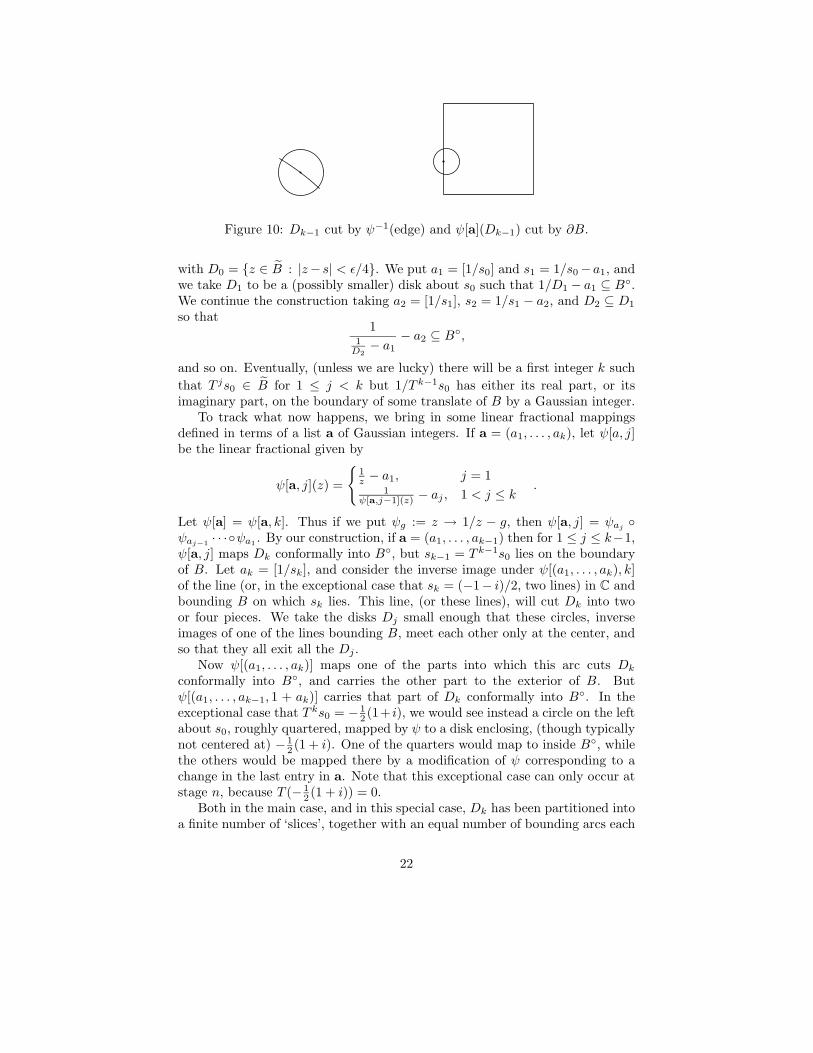
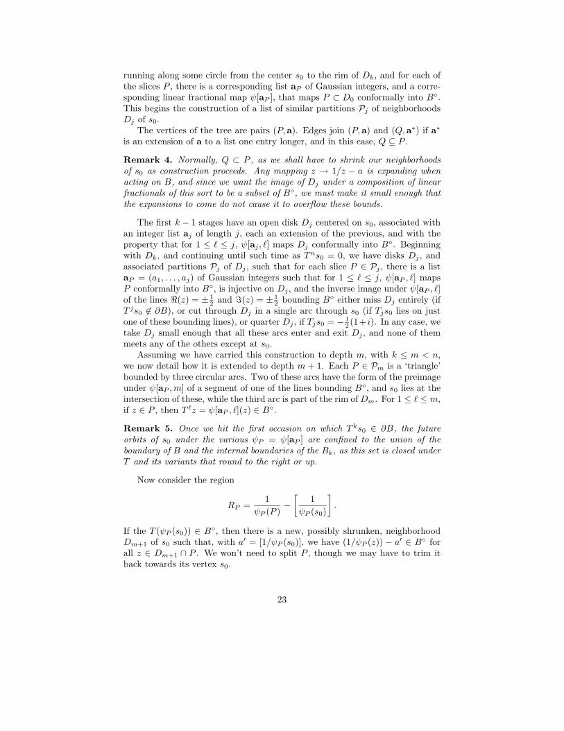
Figure 10: Dk−1 cut by ψ−1(edge) and ψ[a](Dk−1) cut by ∂B.

with D0 = {z ∈ B : |z− s| < ǫ/4}. We put a1 = [1/s0] and s1 = 1/s0 −a1, andwe take D1 to be a (possibly smaller) disk about s0 such that 1/D1 − a1 ⊆ B◦.We continue the construction taking a2 = [1/s1], s2 = 1/s1 − a2, and D2 ⊆ D1

so that1

1D2

− a1

− a2 ⊆ B◦,

and so on. Eventually, (unless we are lucky) there will be a first integer k such

that T js0 ∈ B for 1 ≤ j < k but 1/T k−1s0 has either its real part, or itsimaginary part, on the boundary of some translate of B by a Gaussian integer.

To track what now happens, we bring in some linear fractional mappingsdefined in terms of a list a of Gaussian integers. If a = (a1, . . . , ak), let ψ[a, j]be the linear fractional given by

ψ[a, j](z) =

{1z − a1, j = 1

1ψ[a,j−1](z) − aj , 1 < j ≤ k

.

Let ψ[a] = ψ[a, k]. Thus if we put ψg := z → 1/z − g, then ψ[a, j] = ψaj◦

ψaj−1· · ·◦ψa1

. By our construction, if a = (a1, . . . , ak−1) then for 1 ≤ j ≤ k−1,ψ[a, j] maps Dk conformally into B◦, but sk−1 = T k−1s0 lies on the boundaryof B. Let ak = [1/sk], and consider the inverse image under ψ[(a1, . . . , ak), k]of the line (or, in the exceptional case that sk = (−1− i)/2, two lines) in C andbounding B on which sk lies. This line, (or these lines), will cut Dk into twoor four pieces. We take the disks Dj small enough that these circles, inverseimages of one of the lines bounding B, meet each other only at the center, andso that they all exit all the Dj .

Now ψ[(a1, . . . , ak)] maps one of the parts into which this arc cuts Dk

conformally into B◦, and carries the other part to the exterior of B. Butψ[(a1, . . . , ak−1, 1 + ak)] carries that part of Dk conformally into B◦. In theexceptional case that T ks0 = − 1

2 (1+ i), we would see instead a circle on the leftabout s0, roughly quartered, mapped by ψ to a disk enclosing, (though typicallynot centered at) − 1

2 (1 + i). One of the quarters would map to inside B◦, whilethe others would be mapped there by a modification of ψ corresponding to achange in the last entry in a. Note that this exceptional case can only occur atstage n, because T (− 1

2 (1 + i)) = 0.Both in the main case, and in this special case, Dk has been partitioned into

a finite number of ‘slices’, together with an equal number of bounding arcs each

22

running along some circle from the center s0 to the rim of Dk, and for each ofthe slices P , there is a corresponding list aP of Gaussian integers, and a corre-sponding linear fractional map ψ[aP ], that maps P ⊂ D0 conformally into B◦.This begins the construction of a list of similar partitions Pj of neighborhoodsDj of s0.

The vertices of the tree are pairs (P,a). Edges join (P,a) and (Q,a∗) if a∗

is an extension of a to a list one entry longer, and in this case, Q ⊆ P .

Remark 4. Normally, Q ⊂ P , as we shall have to shrink our neighborhoodsof s0 as construction proceeds. Any mapping z → 1/z − a is expanding whenacting on B, and since we want the image of Dj under a composition of linearfractionals of this sort to be a subset of B◦, we must make it small enough thatthe expansions to come do not cause it to overflow these bounds.

The first k − 1 stages have an open disk Dj centered on s0, associated withan integer list aj of length j, each an extension of the previous, and with theproperty that for 1 ≤ ℓ ≤ j, ψ[aj , ℓ] maps Dj conformally into B◦. Beginningwith Dk, and continuing until such time as Tns0 = 0, we have disks Dj , andassociated partitions Pj of Dj , such that for each slice P ∈ Pj , there is a listaP = (a1, . . . , aj) of Gaussian integers such that for 1 ≤ ℓ ≤ j, ψ[aP , ℓ] mapsP conformally into B◦, is injective on Dj , and the inverse image under ψ[aP , ℓ]of the lines ℜ(z) = ± 1

2 and ℑ(z) = ± 12 bounding B◦ either miss Dj entirely (if

T js0 6∈ ∂B), or cut through Dj in a single arc through s0 (if Tjs0 lies on justone of these bounding lines), or quarter Dj , if Tjs0 = − 1

2 (1+ i). In any case, wetake Dj small enough that all these arcs enter and exit Dj , and none of themmeets any of the others except at s0.

Assuming we have carried this construction to depth m, with k ≤ m < n,we now detail how it is extended to depth m + 1. Each P ∈ Pm is a ‘triangle’bounded by three circular arcs. Two of these arcs have the form of the preimageunder ψ[aP ,m] of a segment of one of the lines bounding B◦, and s0 lies at theintersection of these, while the third arc is part of the rim of Dm. For 1 ≤ ℓ ≤ m,if z ∈ P , then T ℓz = ψ[aP , ℓ](z) ∈ B◦.

Remark 5. Once we hit the first occasion on which T ks0 ∈ ∂B, the futureorbits of s0 under the various ψP = ψ[aP ] are confined to the union of theboundary of B and the internal boundaries of the Bk, as this set is closed underT and its variants that round to the right or up.

Now consider the region

RP =1

ψP (P )−

[1

ψP (s0)

].

If the T (ψP (s0)) ∈ B◦, then there is a new, possibly shrunken, neighborhoodDm+1 of s0 such that, with a′ = [1/ψP (s0)], we have (1/ψP (z)) − a′ ∈ B◦ forall z ∈ Dm+1 ∩ P . We won’t need to split P , though we may have to trim itback towards its vertex s0.

23

If, on the other hand, b = 1/ψP (s0) − a′ ∈ ∂B, we introduce a new arccutting Dm through s0. This arc is the inverse image under z → 1/ψP (z) − a′

of the line bounding B◦ on which b lies. Say that an arc α cuts P if it meetsP in any neighborhood of s0. Our new arc may or may not cut P . If it doesnot cut P , we take a suitably shrunken portion of P about s0 to be one of thepieces of Pm+1, and we extend the Gaussian integer list a by appending a′, toprovide the pair (P,a′) say. If it does cut P , we take suitably shrunken portionsof the two sectors into which the portion of P near s0 has been cut by our arc,to be the two pieces in Pm+1 corresponding to P .

One of these pieces will be associated with the same extension of a we usedbefore, while for the other, we extend instead by a′ +1, if b was on the left edgeof B, or by a′+i, if b was on the bottom edge of B. We now further truncate ourslices, if necessary, to a radius which is the minimum of the radii of the pieces wegot during the construction of Pm+1. The union of these pieces, together withtheir internal boundaries with each other, is now a pie-slice partition of an opendisk Dm+1 centered on s0, and for each P ∈ Pm+1, there is a correspondingGaussian integer list a, an extension of the one that was associated with theparent P in Pm, such that ψ[a, ℓ] maps P into B◦ for 1 ≤ ℓ ≤ m + 1.

We now claim that for all P ∈ Pn−1, 1/ψ[aP ](s0) ∈ G′. That is, the variantsof the algorithm all run to completion on Gaussian rational input in the samenumber of steps. The reason for this is symmetry. The group S of rigid motionstaking B onto B is generated by λ1(z) = z and λ2(z) = iz. We consider theequivalence relation ∼ on C determined by u ∼ v if u = λv for some λ ∈ S.

If z ∼ w then 1/z ∼ 1/w, and if z, w ∈ B and z ∼ w, and if a, b ∈ G′ suchthat 1/z − a ∈ B and 1/w − b ∈ B, then 1/z − a ∼ 1/w − b. Initially, s0 ∼ s0.If ψ[a1, ℓ](s0) = sl ∼ ψ[a2, ℓ](s0) = s′l for all pairs (a1,a2) of lists of length ℓoccurring in the disk partition tree of s0, then 1/sℓ ∼ 1/sℓ′ , and now for any ofthe choices a∗ by which a1 may be extended,the various 1/sℓ−a∗ are equivalentunder ∼ to each other, and to the complex numbers that may arise out of 1/sℓ′

by extending a2 with a∗∗, say. (Another way to say this is to say that if weidentified all elements of a given equivalence class under ∼, all the variants ofT would condense to one.)

At the end, when sn−1 ∈ 1/G′, all other s ∼ sn−1 also belong to 1/G′, so Tmaps them to zero as well. Therefore, all branches of our disk partition tree fors0 have the same depth.

Now for each (P,aP ) of depth n in our disk partition tree,

ψ[a, n](z) =

(1

z− an

)◦

(1

z− an−1

)· · · ◦

(1

z− a1

)

takes s0 to 0, and takes P on an orbit that at each stage remains inside B◦.Since these slices P partition the final disk Dn about s0 into a finite number

of slices, and since the sum of the angles at s0 of the slices is 2π, there must beat least one slice that occupies a positive angle at s0. Let P ′ be such a slice,and a

′ its Gaussian integer list. The image under ψ[a′] of P is a ‘triangle’ inB◦ with its vertex ψ[a′](s0) = 0 with a positive angle at 0. For all z ∈ P ′,Tnz = ψ[a′](z). Our disk partition tree has now served its purpose.

24

There are Gaussian integers g ∈ G′ such that 1/g ∈ P ′. Any neighborhoodE of 1/g contained in P ′ will be taken conformally under z → 1/z − g to a

neighborhood E of 0. We take another Gaussian integer h such that 1/(h+B) ⊆E, and such that 1/(h + B) is also a subset of some particular Br. Let a be thelist got by appending g and then h to a

′. Now let r = ψ[a′]−1(1/(g + 1/h)) =ψ[a]−1(0), and let

D ⊂ Dn = ψ[a′]−1 ◦(

1

z + g

)◦

(1

z + h

)B◦.

Iterating T takes D conformally to various squarish neighborhoods inside B◦,until Tn+1 takes it to the squarish region (1/(h + B◦)) ⊂ E, and finally Tn+2

carries it via z → 1/z − h onto B◦.

A bit more is true. The orbit of D never meets any of the internal boundariesseparating the various Bk until the last step, when it is splashed across B◦. Thisis because if, at any earlier point any part of the orbit had touched an internalboundary, the subsequent iterations of T on that point would have also been inthe union of these internal boundaries with the boundary of B itself, and yet,at the stage immediately prior to the final one, no point of Tn+1D belongs toany of these boundaries.

Now that we have our magic r, we are in a position to complete the proofthat LT is u0-positive with u0 ≡ 1. If f 6= 0 ∈ V, and f ≥ 0, then thereexists s ∈ B such that f(s) > 0. We choose an open disk D0 around s suchthat D0 ⊂ Bk where Bk is the one containing s, and such that for z ∈ D0,f(z) > 1

2f(s). Now for z ∈ B, (Ln+2T f)(z) is a sum of terms, among which

(keeping in mind that [c1, c2, . . . , ck] = 1/(c1 + 1/(c2 + . . . + 1/ck))) is the term

n+2∏

j=1

|[aj , . . . , an+2 + z]|4 f([〈an+2, an+1, . . . , a2, a1 + z〉]).

But for arbitrary z ∈ B◦, the argument of f lies inside D0, and the productis bounded below by a positive constant on B◦, so this term is bounded belowby a positive constant on B ⊂ B◦. Since LT is a bounded linear operator, weare almost done. We have proved most of the claims in our Gauss-Kuz’mintheorem.

For the symmetry claims, we first note that ρ(z) = ρ(z). Suppose not. Letρ1(z) = ρ(z)−ρ(iz). Then LT ρ1 = ρ1. But

∫B

ρ1 = 0, so ρ1 must be identically

zero on B. For mirror symmetry, let ρ2(z) = ρ(z) − ρ(z). Then

LT ρ2(z) =∑

g∈G′

|g + z|−4 (ρ(1/(g + z)) − ρ(1/(g + z)))

= ρ(z) − LT ρ(z) = ρ(z) − ρ(z) = ρ2(z).

As before,∫

Bρ2 = 0, so ρ2 is the zero element of V. This completes the proof

of our Gauss-Kuz’min theorem.

25

References

[1] Bandtlow, O. and Jenkinson, O. Invariant measures for real analytic ex-panding maps (to appear).

[2] Hurwitz, A. (1888). Uber die Entwicklung Complexer Grossen in Ket-tenbruche, Acta Math. 11, pp. 187-200.

[3] Hurwitz, J. (1895) Uber eine besondere Art der Kettenbruch-entwicklungcomplexer Grossen, Thesis, Universitat Halle-Wittenberg, Halle, Germany.

[4] Krasnoselskii, M. (1964). Positive solutions of operator equations. P. Noord-hoff, Groningen.

[5] Lagarias, J. (1994). Geodesic multidimensional continued fractions, Proc.London Math. Soc. 3, 69, pp. 464-488.

[6] Narasimhan, R. (1971). Several Complex Variables, University of ChicagoPress, Chicago.

[7] Schmidt, A. (1975). Diophantine approximation of complex numbers. ActaMath. 134, pp. 1-85.

26