The Geometry of the TDOA based Source Localization TDOA{based Localization Problem: point-like...

Geometry ofTDOA–basedSource

Localization

MarcoCompagnoni

Introduction

The TDOAMap

TheMultilinearAlgebraSolution

The Imageof τ2 andtheBifurcationProblem

ThecompleteTDOA mapand sketchesabout τ3

ConclusionsandPerspectives

Extra

The Geometry of the TDOA–based SourceLocalization

Marco Compagnoni

SIAM Conference on Applied Algebraic Geometry

Fort Collins

August 3, 2013


Localization

MarcoCompagnoni

Introduction

The TDOAMap





Extra

Joint work with Roberto Notari, Fabio Antonacci, Augusto Sarti.


Localization

MarcoCompagnoni

Introduction

The TDOAMap





Extra

2D TDOA–based Localization

Problem: point-like (acoustic) source localization based on thetime differences of arrival (TDOA) of a signal to distinctreceivers lying on a plane.

Experimental data:the TDOAs τji of the signal toreceivers mj and mi, measuredas the time shifts of the signalwavefront.

Goal: obtain a complete description of the statistical modelbehind TDOA-based source localization, possibly withunsynchronized and uncalibrated receivers.


Localization

MarcoCompagnoni

Introduction

The TDOAMap





Extra

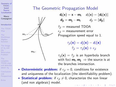
The Geometric Propagation Model

m0m1

m2

x

di(x) = x−mi di (x) = ‖di(x)‖dji = mj −mi dji = ‖dji‖

τji = measured TDOAεji = measurement errorPropagation speed equal to 1.

τji(x) = dj(x)− di(x)

τji = τij(x) + εji

τij(x) = τji is an hyperbola branchwith foci mi,mj ⇒ the source is atthe branches intersection.

• Deterministic problem: if εji = 0, conditions for existenceand uniqueness of the localization (the identifiability problem).

• Statistical problem: if εji 6= 0, characterize the non linear(and non algebraic) model.


Localization

MarcoCompagnoni

Introduction

The TDOAMap





Extra

The GPS ProblemIn the classical GPS problem one searches the location of asource in space using the times of arrival ti of signals (TOAs)from n distinct satellites to the GPS receiver.

The TOA Model: ti(x) = di(x) + εi + b

• Because of the low accuracy of the receiver clock, onehas to consider an additional bias b for each TOA.

• In order to eliminate b, one chooses a reference satellitem1 and takes as input data the differences ti(x)− t1(x).

In the deterministic case the GPS problem reduces tothe TDOA-based localization.

• Existence problem: how many satellites are necessaryto locate a source?

• Uniqueness or Bifurcation problem: in which cases isthe localization unique?


Localization

MarcoCompagnoni

Introduction

The TDOAMap





Extra

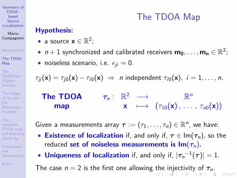
The TDOA Map

Hypothesis:

• a source x ∈ R2;

• n + 1 synchronized and calibrated receivers m0, . . . ,mn ∈ R2;

• noiseless scenario, i.e. εji = 0.

τji (x) = τj0(x)− τi0(x) ⇒ n independent τi0(x), i = 1, . . . , n.

The TDOA τn : R2 −→ Rn

map x 7−→ (τ10(x) , . . . , τn0(x))

Given a measurements array τ := (τ1, . . . , τn) ∈ Rn, we have:

• Existence of localization if, and only if, τ ∈ Im(τn), so thereduced set of noiseless measurements is Im(τn).

• Uniqueness of localization if, and only if, |τn−1(τ )| = 1.

The case n = 2 is the first one allowing the injectivity of τn.


Localization

MarcoCompagnoni

Introduction

The TDOAMap





Extra

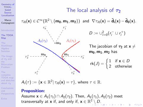
The local analysis of τ2

τi0(x) ∈ C∞(R2 \ {m0,m1,m2}) and ∇τi0(x) = di(x)− d0(x).

r+2 r−2

r+1

r−1

r+0

r−0

m0 m1

m2A2(τ2) A1(τ1)

D := ∪2i=0(r−i ∪ r+i )

The jacobian of τ2 at x 6=m0,m1,m2 has

rk(J) =

{1 if x ∈ D2 otherwise

Ai (τ) := {x ∈ R2| τi0(x) = τ}, where τ ∈ R.

Proposition:Assume x ∈ A1(τ1) ∩ A2(τ2). Then, A1(τ1),A2(τ2) meettransversally at x if, and only if, x ∈ R2 \ D.


Localization

MarcoCompagnoni

Introduction

The TDOAMap





Extra

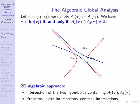
The Algebraic Global AnalysisLet τ = (τ1, τ2), we denote Ai (τ ) := Ai (τi ). We haveτ ∈ Im(τ2) if, and only if, A1(τ ) ∩ A2(τ ) 6= ∅.

m0 m1

m2

2D algebraic approach:

• Intersection of the two hyperbolas containing A1(τ ),A2(τ ).

• Problems: extra intersections, complex intersections.


Localization

MarcoCompagnoni

Introduction

The TDOAMap





Extra

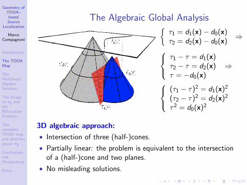
The Algebraic Global Analysis{τ1 = d1(x)− d0(x)τ2 = d2(x)− d0(x)

⇒

τ1 − τ = d1(x)τ2 − τ = d2(x)τ = −d0(x)

⇒

(τ1 − τ)2 = d1(x)2

(τ2 − τ)2 = d2(x)2

τ2 = d0(x)2

3D algebraic approach:

• Intersection of three (half-)cones.

• Partially linear: the problem is equivalent to the intersectionof a (half-)cone and two planes.

• No misleading solutions.


Localization

MarcoCompagnoni

Introduction

The TDOAMap





Extra

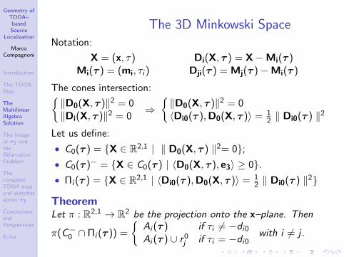
The 3D Minkowski SpaceNotation:

X = (x, τ) Di(X, τ ) = X−Mi(τ )Mi(τ ) = (mi, τi ) Dji(τ ) = Mj(τ )−Mi(τ )

The cones intersection:{‖D0(X, τ )‖2 = 0‖Di(X, τ )‖2 = 0

⇒{‖D0(X, τ )‖2 = 0〈Di0(τ ),D0(X, τ )〉 = 1

2 ‖ Di0(τ ) ‖2

Let us define:

• C0(τ ) = {X ∈ R2,1 | ‖ D0(X, τ ) ‖2= 0};• C0(τ )− = {X ∈ C0(τ ) | 〈D0(X, τ ), e3〉 ≥ 0}.• Πi (τ ) = {X ∈ R2,1 | 〈Di0(τ ),D0(X, τ )〉 = 1

2 ‖ Di0(τ ) ‖2}

TheoremLet π : R2,1 → R2 be the projection onto the x–plane. Then

π(C−0 ∩ Πi (τ )) =

{Ai (τ ) if τi 6= −di0Ai (τ ) ∪ r0j if τi = −di0

with i 6= j .


Localization

MarcoCompagnoni

Introduction

The TDOAMap





Extra

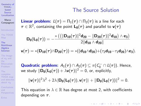
The Source Solution

Linear problem: L(τ ) = Π1(τ ) ∩ Π2(τ ) is a line for eachτ ∈ R2, containing the point L0(τ ) and parallel to v(τ )

D0(L0(τ )) = −∗((‖D10(τ )‖2d20 − ‖D20(τ )‖2d10

)∧ e3

)2‖d10 ∧ d20‖

v(τ ) = ∗(D10(τ )∧D20(τ )) = ∗((d10∧d20)+(τ2d10−τ1d20)∧e3).

Quadratic problem: A1(τ ) ∩ A2(τ ) ⊆ π(C−0 ∩ L(τ )). Hence,we study ‖D0(L0(τ )) + λv(τ )‖2 = 0, or, explicitly,

‖v(τ )‖2λ2 + 2λ〈D0(L0(τ )), v(τ )〉+ ‖D0(L0(τ ))‖2 = 0.

This equation in λ ∈ R has degree at most 2, with coefficientsdepending on τ .


Localization

MarcoCompagnoni

Introduction

The TDOAMap





Extra

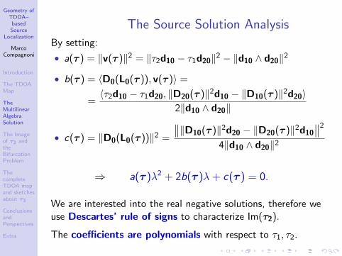
The Source Solution Analysis

By setting:

• a(τ ) = ‖v(τ )‖2 = ‖τ2d10 − τ1d20‖2 − ‖d10 ∧ d20‖2

• b(τ ) = 〈D0(L0(τ )), v(τ )〉 =

=〈τ2d10 − τ1d20, ‖D20(τ )‖2d10 − ‖D10(τ )‖2d20〉

2‖d10 ∧ d20‖

• c(τ ) = ‖D0(L0(τ ))‖2 =

∥∥‖D10(τ )‖2d20 − ‖D20(τ )‖2d10

∥∥24‖d10 ∧ d20‖2

⇒ a(τ )λ2 + 2b(τ )λ + c(τ ) = 0.

We are interested into the real negative solutions, therefore weuse Descartes’ rule of signs to characterize Im(τ2).

The coefficients are polynomials with respect to τ1, τ2.


Localization

MarcoCompagnoni

Introduction

The TDOAMap





Extra

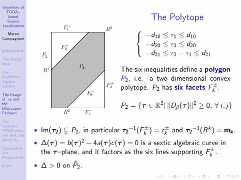
The Polytope

F−2

F+1

F+2

F−1

F+0

F−0

P2

R0

R1

R2

−d10 ≤ τ1 ≤ d10−d20 ≤ τ2 ≤ d20−d21 ≤ τ2 − τ1 ≤ d21

The six inequalities define a polygonP2, i.e. a two dimensional convexpolytope. P2 has six facets F±k .

P2 = {τ ∈ R2| ‖Dji (τ )‖2 ≥ 0, ∀ i , j}

• Im(τ2) ( P2, in particular τ2−1(F±k ) = r±k and τ2

−1(Rk) = mk.

• ∆(τ ) = b(τ )2 − 4a(τ )c(τ ) = 0 is a sextic algebraic curve inthe τ–plane, and it factors as the six lines supporting F±k .

• ∆ > 0 on P2.


Localization

MarcoCompagnoni

Introduction

The TDOAMap





Extra

The analysis of the coefficients

R0

R01

R∗

R∗1

Co

E

c =‖‖D10(τ )‖2d20−‖D20(τ )‖2d10‖2

4‖d10∧d20‖2

• c(τ ) = 0 iff τ ∈ {R0,R∗,R∗1 ,R01},

• c(τ ) > 0 otherwise.

a = ‖τ2d10 − τ1d20‖2 − ‖d10 ∧ d20‖2

• a = 0 is the unique ellipse Etangent to each facet of P2,

• a < 0 inside E and a > 0 outside.

b(τ ) = 〈τ2d10−τ1d20,‖D20(τ )‖2d10−‖D10(τ )‖2d20〉2‖d10∧d20‖

• b = 0 is the unique cubic C through the 11 marked points,

• only the odd circuit Co of C contains the 11 points, while theeven circuit Ce (if it exists) does not intersect P2.


Localization

MarcoCompagnoni

Introduction

The TDOAMap





Extra

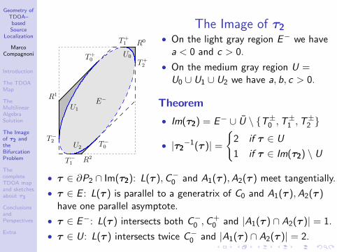
The Image of τ2

R0

R1

R2

T+1

T−1

T+2

T−2

T+0

T−0

E−

U0

U1

U2

• On the light gray region E− we havea < 0 and c > 0.

• On the medium gray region U =U0 ∪ U1 ∪ U2 we have a, b, c > 0.

Theorem

• Im(τ2) = E− ∪ U \ {T±0 ,T±1 ,T

±2 }

• |τ2−1(τ )| =

{2 if τ ∈ U

1 if τ ∈ Im(τ2) \ U

• τ ∈ ∂P2 ∩ Im(τ2): L(τ ),C−0 and A1(τ ),A2(τ ) meet tangentially.

• τ ∈ E : L(τ ) is parallel to a generatrix of C0 and A1(τ ),A2(τ )have one parallel asymptote.

• τ ∈ E−: L(τ ) intersects both C−0 ,C+0 and |A1(τ ) ∩ A2(τ )| = 1.

• τ ∈ U: L(τ ) intersects twice C−0 and |A1(τ ) ∩ A2(τ )| = 2.


Localization

MarcoCompagnoni

Introduction

The TDOAMap





Extra

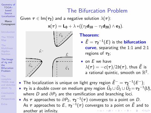
The Bifurcation ProblemGiven τ ∈ Im(τ2) and a negative solution λ(τ ):

x(τ ) = L0 + λ ∗((τ2d10 − τ1d20) ∧ e3).

Theorem:

• E = τ2−1(E ) is the bifurcation

curve, separating the 1:1 and 2:1regions of τ2;

• on E we haveλ(τ ) = −c(τ )/2b(τ ), thus E isa rational quintic, smooth on R2.

• The localization is unique on light grey region E− = τ2−1(E−);

• τ2 is a double cover on medium grey region U0 ∪ U1 ∪ U2 =τ2−1(U),

where D and ∂P2 are the ramification and branching loci.• As τ approaches to ∂P2, τ2

−1(τ ) converges to a point on D.As τ approaches to E , τ2

−1(τ ) converges to a point on E and toanother at infinity.


Localization

MarcoCompagnoni

Introduction

The TDOAMap





Extra

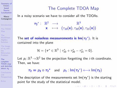
The Complete TDOA Map

In a noisy scenario we have to consider all the TDOAs.

τ2∗ : R2 −→ R3

x 7−→ (τ10(x), τ20(x), τ21(x))

The set of noiseless measurements is Im(τ2∗). It is

contained into the plane

H = {τ ∗ ∈ R3 | τ∗10 + τ∗20 − τ∗21 = 0}.

Let pi :R3→R2 be the projection forgetting the i-th coordinate.Then, we have:

τ2 = p3 ◦ τ2∗ and p3 : Im(τ2

∗)←→ Im(τ2)

The description of the measurements set Im(τ2∗) is the starting

point for the study of the statistical model.


Localization

MarcoCompagnoni

Introduction

The TDOAMap





Extra

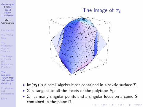
The Image of τ3

• Im(τ3) is a semi–algebraic set contained in a sextic surface Σ.

• Σ is tangent to all the facets of the polytope P3.

• Σ has many singular points and a singular locus on a conic Scontained in the plane Π.


Localization

MarcoCompagnoni

Introduction

The TDOAMap





Extra

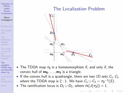
The Localization Problem

• The TDOA map τ3 is a homeomorphism if, and only if, theconvex hull of m0, . . . ,m3 is a triangle.

• If the convex hull is a quadrangle, there are two 1D sets C1,C2

where the TDOA map is 2 : 1. We have C1 ∪ C2 = τ3−1(S).

• The ramification locus is D1 ∪ D2, where rk(J(τ3)) = 1.


Localization

MarcoCompagnoni

Introduction

The TDOAMap





Extra

Conclusions and Perspectives

In this work:

• we studied the planar TDOA-based localization problem withthree receivers in a noiseless scenario;

• in particular we have characterized the measurements spaceand the bifurcation curve in terms of real (semi)algebraic sets;

• we introduced the complete measurements space.

In future works we will:

• complete the cases n ≥ 3;

• study the 3-dimensional TDOA-based localization;

• study the statistical properties of the model.


Localization

MarcoCompagnoni

Introduction

The TDOAMap





Extra

Bibliography

M.Compagnoni, P.Bestagini, F.Antonacci, A.Sarti,S.Tubaro, Localization of Acoustic Sources Through theFitting of Propagation Cones Using Multiple IndependentArrays, IEEE Transactions on Audio, Speech, and LanguageProcessing, Vol. 20 (2012), Issue 7, 1964–1975.

P.Bestagini, M.Compagnoni, F.Antonacci, A.Sarti,S.Tubaro, TDOA-Based Acoustic Source Localization in theSpace–Range Reference Frame, to appear inMultidimensional Systems and Signal Processing.

B.Coll, J.J.Ferrando, J.A.Morales-Lladosaz, Positioningsystems in Minkowski space-time: from emission to inertialcoordinates, Class.Quant.Grav. 27, 065013 (2010).

B.Coll, J.J.Ferrando, J.A.Morales-Lladosaz, Positioningsystems in Minkowski space-time: Bifurcation problem andobservational data, arXiv:1204.2241v2 [gr-qc].


Localization

MarcoCompagnoni

Introduction

The TDOAMap





Extra

Geometric Interpretation

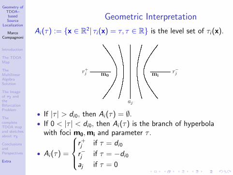
Ai(τ) := {x ∈ R2| τi(x) = τ, τ ∈ R} is the level set of τi(x).

r+j r−j

aj

m0 mi

• If |τ | > di0, then Ai(τ) = ∅.• If 0 < |τ | < di0, then Ai(τ) is the branch of hyperbola

with foci m0,mi and parameter τ .

• Ai(τ) =

r+j if τ = di0r−j if τ = −di0aj if τ = 0


Localization

MarcoCompagnoni

Introduction

The TDOAMap





Extra

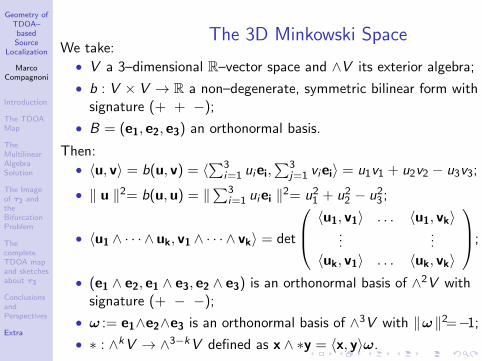
The 3D Minkowski SpaceWe take:• V a 3–dimensional R–vector space and ∧V its exterior algebra;

• b : V × V → R a non–degenerate, symmetric bilinear form withsignature (+ + −);

• B = (e1, e2, e3) an orthonormal basis.

Then:• 〈u, v〉 = b(u, v) = 〈

∑3i=1 uiei,

∑3j=1 viei〉 = u1v1 + u2v2 − u3v3;

• ‖ u ‖2= b(u,u) = ‖∑3

i=1 uiei ‖2= u21 + u22 − u23 ;

• 〈u1 ∧ · · · ∧ uk, v1 ∧ · · · ∧ vk〉 = det

〈u1, v1〉 . . . 〈u1, vk〉...

...〈uk, v1〉 . . . 〈uk, vk〉

;

• (e1 ∧ e2, e1 ∧ e3, e2 ∧ e3) is an orthonormal basis of ∧2V withsignature (+ − −);

• ω := e1∧e2∧e3 is an orthonormal basis of ∧3V with ‖ω‖2=−1;

• ∗ : ∧kV → ∧3−kV defined as x ∧ ∗y = 〈x, y〉ω.


Localization

MarcoCompagnoni

Introduction

The TDOAMap





Extra

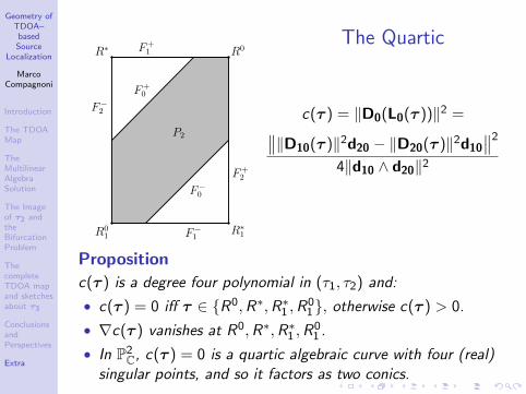
The Quartic

F−2

F+1

F+2

F−1

F+0

F−0

P2

R0

R01

R∗

R∗1

c(τ ) = ‖D0(L0(τ ))‖2 =∥∥‖D10(τ )‖2d20 − ‖D20(τ )‖2d10

∥∥24‖d10 ∧ d20‖2

Proposition

c(τ ) is a degree four polynomial in (τ1, τ2) and:

• c(τ ) = 0 iff τ ∈ {R0,R∗,R∗1 ,R01}, otherwise c(τ ) > 0.

• ∇c(τ ) vanishes at R0,R∗,R∗1 ,R01 .

• In P2C, c(τ ) = 0 is a quartic algebraic curve with four (real)

singular points, and so it factors as two conics.


Localization

MarcoCompagnoni

Introduction

The TDOAMap





Extra

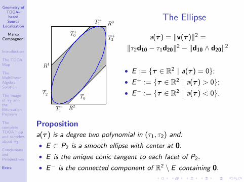
The EllipseR0

R1

R2

T+1

T−1

T+2

T−2

T+0

T−0

a(τ ) = ‖v(τ )‖2 =

‖τ2d10 − τ1d20‖2 − ‖d10 ∧ d20‖2

• E := {τ ∈ R2 | a(τ ) = 0};• E+ := {τ ∈ R2 | a(τ ) > 0};• E− := {τ ∈ R2 | a(τ ) < 0}.

Proposition

a(τ ) is a degree two polynomial in (τ1, τ2) and:

• E ⊂ P2 is a smooth ellipse with center at 0.

• E is the unique conic tangent to each facet of P2.

• E− is the connected component of R2 \ E containing 0.


Localization

MarcoCompagnoni

Introduction

The TDOAMap





Extra

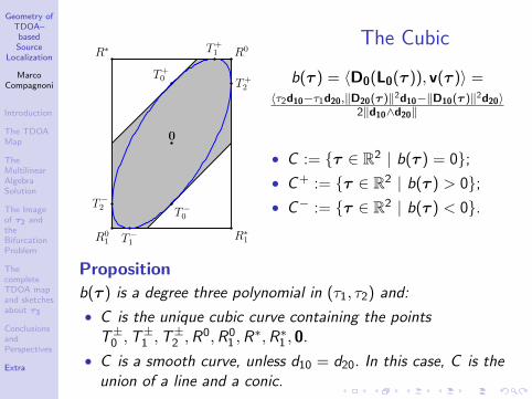
The CubicR0

R01

R∗

R∗1

T+1

T−1

T+2

T−2

T+0

T−0

0

b(τ ) = 〈D0(L0(τ )), v(τ )〉 =〈τ2d10−τ1d20,‖D20(τ )‖2d10−‖D10(τ )‖2d20〉

2‖d10∧d20‖

• C := {τ ∈ R2 | b(τ ) = 0};• C+ := {τ ∈ R2 | b(τ ) > 0};• C− := {τ ∈ R2 | b(τ ) < 0}.

Proposition

b(τ ) is a degree three polynomial in (τ1, τ2) and:

• C is the unique cubic curve containing the pointsT±0 ,T

±1 ,T

±2 ,R

0,R01 ,R

∗,R∗1 , 0.

• C is a smooth curve, unless d10 = d20. In this case, C is theunion of a line and a conic.


Localization

MarcoCompagnoni

Introduction

The TDOAMap





Extra

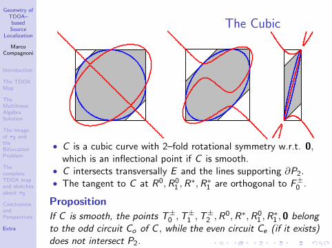
The Cubic

• C is a cubic curve with 2–fold rotational symmetry w.r.t. 0,which is an inflectional point if C is smooth.

• C intersects transversally E and the lines supporting ∂P2.• The tangent to C at R0,R0

1 ,R∗,R∗1 are orthogonal to F±0 .

Proposition

If C is smooth, the points T±0 ,T±1 ,T

±2 ,R

0,R∗,R01 ,R

∗1 , 0 belong

to the odd circuit Co of C , while the even circuit Ce (if it exists)does not intersect P2.


Localization

MarcoCompagnoni

Introduction

The TDOAMap





Extra

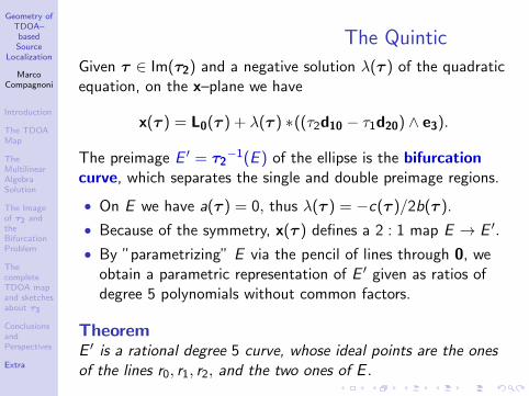
The Quintic

Given τ ∈ Im(τ2) and a negative solution λ(τ ) of the quadraticequation, on the x–plane we have

x(τ ) = L0(τ ) + λ(τ ) ∗((τ2d10 − τ1d20) ∧ e3).

The preimage E ′ = τ2−1(E ) of the ellipse is the bifurcation

curve, which separates the single and double preimage regions.

• On E we have a(τ ) = 0, thus λ(τ ) = −c(τ )/2b(τ ).

• Because of the symmetry, x(τ ) defines a 2 : 1 map E → E ′.

• By ”parametrizing” E via the pencil of lines through 0, weobtain a parametric representation of E ′ given as ratios ofdegree 5 polynomials without common factors.

TheoremE ′ is a rational degree 5 curve, whose ideal points are the onesof the lines r0, r1, r2, and the two ones of E .


Localization

MarcoCompagnoni

Introduction

The TDOAMap





Extra

The Quintic

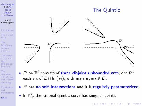
E ′E ′

• E ′ on R2 consists of three disjoint unbounded arcs, one foreach arc of E ∩ Im(τ2), with m0,m1,m2 6∈ E ′.

• E ′ has no self–intersections and it is regularly parameterized.

• In P2C, the rational quintic curve has singular points.


Localization

MarcoCompagnoni

Introduction

The TDOAMap





Extra

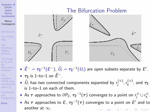
The Bifurcation Problem

• E− = τ2−1(E−), Ui = τ2

−1(Ui ) are open subsets separate by E ′.

• τ2 is 1–to–1 on E−.

• Ui has two connected components separeted by r(±)j , r

(±)k , and τ2

is 1–to–1 on each of them.

• As τ approaches to ∂P2, τ2−1(τ ) converges to a point on r±j ∪ r

±k .

• As τ approaches to E , τ2−1(τ ) converges to a point on E ′ and to

another at ∞.


Localization

MarcoCompagnoni

Introduction

The TDOAMap





Extra

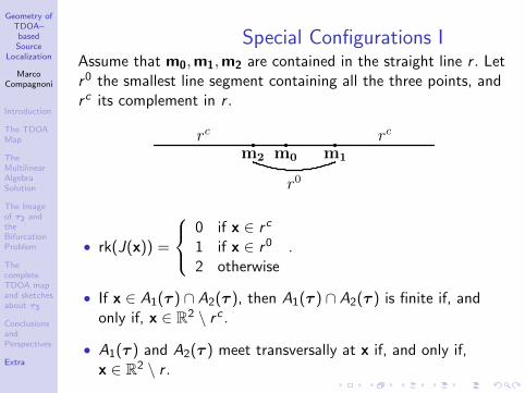
Special Configurations IAssume that m0,m1,m2 are contained in the straight line r . Letr0 the smallest line segment containing all the three points, andr c its complement in r .

m2 m0 m1

r0

rc rc

• rk(J(x)) =

0 if x ∈ r c

1 if x ∈ r0

2 otherwise.

• If x ∈ A1(τ ) ∩ A2(τ ), then A1(τ ) ∩ A2(τ ) is finite if, andonly if, x ∈ R2 \ r c .

• A1(τ ) and A2(τ ) meet transversally at x if, and only if,x ∈ R2 \ r .


Localization

MarcoCompagnoni

Introduction

The TDOAMap





Extra

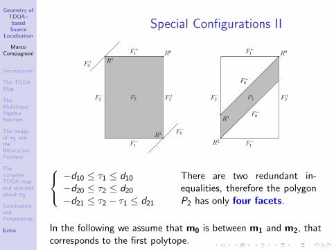
Special Configurations II

F−2

F+1

F+2

F−1

F+0

F−0

P2

R0

R1

R2

F−2

F+1

F+2

F−1

F+0

F−0

P2

R0

R1

R2

−d10 ≤ τ1 ≤ d10−d20 ≤ τ2 ≤ d20−d21 ≤ τ2 − τ1 ≤ d21

There are two redundant in-equalities, therefore the polygonP2 has only four facets.

In the following we assume that m0 is between m1 and m2, thatcorresponds to the first polytope.


Localization

MarcoCompagnoni

Introduction

The TDOAMap





Extra

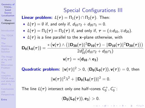
Special Configurations IIILinear problem: L(τ ) = Π1(τ ) ∩ Π2(τ ). Then:

• L(τ ) = ∅ if, and only if, d10τ2 + d20τ1 = 0.

• L(τ ) = Π1(τ ) = Π2(τ ) if, and only if, τ = (±d10,∓d20).

• L(τ ) is a line parallel to the x–plane otherwise, with

D0(L0(τ )) =∗(v(τ ) ∧

(‖D20(τ )‖2D10(τ )− ‖D10(τ )‖2D20(τ )

))2d2

10(d10τ2 + d20τ1)

v(τ ) = ∗(d10 ∧ e3)

Quadratic problem: ‖v(τ )‖2 > 0, 〈D0(L0(τ )), v(τ )〉 = 0, then

‖v(τ )‖2λ2 + ‖D0(L0(τ ))‖2 = 0.

The line L(τ ) intersect only one half–cones C+0 ,C

−0 :

〈D0(L0(τ )), e3〉 > 0.


Localization

MarcoCompagnoni

Introduction

The TDOAMap





Extra

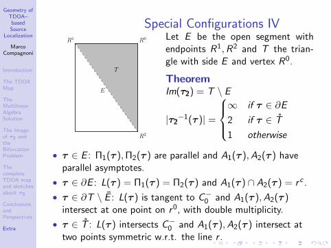
Special Configurations IV

E

R0R1

R2

T

Let E be the open segment withendpoints R1,R2 and T the trian-gle with side E and vertex R0.

TheoremIm(τ2) = T \ E

|τ2−1(τ )| =

∞ if τ ∈ ∂E2 if τ ∈ T

1 otherwise

• τ ∈ E : Π1(τ ),Π2(τ ) are parallel and A1(τ ),A2(τ ) haveparallel asymptotes.

• τ ∈ ∂E : L(τ ) = Π1(τ ) = Π2(τ ) and A1(τ ) ∩ A2(τ ) = r c .

• τ ∈ ∂T \ E : L(τ ) is tangent to C−0 and A1(τ ),A2(τ )intersect at one point on r0, with double multiplicity.

• τ ∈ T : L(τ ) intersects C−0 and A1(τ ),A2(τ ) intersect attwo points symmetric w.r.t. the line r .


Localization

MarcoCompagnoni

Introduction

The TDOAMap





Extra

Restoring the Symmetry I

In the definition of the TDOA map we chose m0 as referencereceiver, breaking the symmetry of the problem.

Dj(X, τ ) = D0(X, τ ) + D0j(τ ) Dij(τ ) = Di0(τ ) + D0j(τ )

Theorem

π(C−0 (τ ) ∩ C−1 (τ ) ∩ C−2 (τ )) = π(C−i (τ ) ∩ Πji (τ ) ∩ Πki (τ ))

In particular the three lines L0(τ ), L1(τ ), L2(τ ) coincide.

v0(τ ) = v1(τ ) = v2(τ ).

D0(L0(τ )) 6= D1(L1(τ )) 6= D2(L2(τ )).

The localization does not depend on the choice of the referencereceiver. What does it happen to the Im(τ2) in the τ–space?


Localization

MarcoCompagnoni

Introduction

The TDOAMap





Extra

Restoring the Symmetry II

The complete τ2∗ : R2 −→ R3

TDOA map x 7−→ (τ10(x), τ20(x), τ21(x))

• H = {τ ∗ ∈ R3 | D01(τ ∗) + D12(τ ∗) + D20(τ ∗) = 0};• P2 = {τ ∗ ∈ H | ‖Dji(τ

∗)‖2 ≥ 0 for every i , j};• E = {τ ∗ ∈ H | ‖v0(τ ∗)‖2 = 0};• Ci = {τ ∗ ∈ H | 〈Di(Li(τ

∗), vi(τ∗)〉 = 0}.

TheoremLet pi :R3→R2 be the projection forgetting the i-th coordinate.

• H is a plane containing the admissible TDOA triples;

• P2 is a polygon such that p3(P2) = P2;

• E is the ellipse tangent to all the sides of P2 and p3(E) = E ;

• Ci is the cubic curve containing E ∩ ∂P2,Ri ,Ri0,Ri∗,Ri∗

1 , 0.

τ2 = p3 ◦ τ2∗ and p3 : Im(τ2

∗)←→ Im(τ2)


Localization

MarcoCompagnoni

Introduction

The TDOAMap





Extra

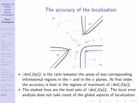
The accuracy of the localization

m0

m1

m2

.02

.02

.05

.05

.1

.1

.1

.1

.5

.5

.5

1

1

11.5

1.5

1.52

2.5

• | det(J(x))| is the ratio between the areas of two correspondinginfinitesimal regions in the τ and in the x planes. At first order,the accuracy is best in the regions of maximum of | det(J(x))|.

• The dashed lines are the level sets of | det(J(x))|. The local erroranalysis does not take count of the global aspects of localization.

The Geometry of the TDOA based Source Localization TDOA{based Localization Problem: point-like...

Documents

Transcript of The Geometry of the TDOA based Source Localization TDOA{based Localization Problem: point-like...