The Framework of Analytic Combinatorics Applied to RNA ... · The Framework of Analytic...
69
The Framework of Analytic Combinatorics Applied to RNA Structures Christie S. Burris Thesis submitted to the Faculty of the Virginia Polytechnic Institute and State University in partial fulfillment of the requirements for the degree of Master of Science in Mathematics Christian Reidys Peter Haskell John Rossi Daniel Orr May 8, 2018 Blacksburg, Virginia Keywords: RNA structures, γ -structures, fatgraphs, Analytic Combinatorics Copyright 2018, Christie Burris
Transcript of The Framework of Analytic Combinatorics Applied to RNA ... · The Framework of Analytic...
The Framework of Analytic Combinatorics Applied to RNAStructures
Christie S. Burris
Thesis submitted to the Faculty of theVirginia Polytechnic Institute and State University
in partial fulfillment of the requirements for the degree of
Master of Sciencein
Mathematics
Christian ReidysPeter HaskellJohn RossiDaniel Orr
May 8, 2018Blacksburg, Virginia
Keywords: RNA structures, γ-structures, fatgraphs, Analytic CombinatoricsCopyright 2018, Christie Burris
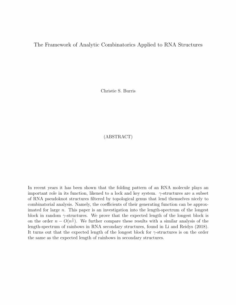
The Framework of Analytic Combinatorics Applied to RNA Structures
Christie S. Burris
(ABSTRACT)
In recent years it has been shown that the folding pattern of an RNA molecule plays animportant role in its function, likened to a lock and key system. γ-structures are a subsetof RNA pseudoknot structures filtered by topological genus that lend themselves nicely tocombinatorial analysis. Namely, the coefficients of their generating function can be approx-imated for large n. This paper is an investigation into the length-spectrum of the longestblock in random γ-structures. We prove that the expected length of the longest block ison the order n − O(n
12 ). We further compare these results with a similar analysis of the
length-spectrum of rainbows in RNA secondary structures, found in Li and Reidys (2018).It turns out that the expected length of the longest block for γ-structures is on the orderthe same as the expected length of rainbows in secondary structures.
The Framework of Analytic Combinatorics Applied to RNA Structures
Christie S. Burris
(GENERAL AUDIENCE ABSTRACT)
Ribonucleic acid (RNA), similar in composition to well-known DNA, plays a myriad of roleswithin the cell. The major distinction between DNA and RNA is the nature of the nucleotidepairings. RNA is single stranded, to mean that its nucleotides are paired with one another(as opposed to a unique complementary strand). Consequently, RNA exhibits a knotted 3Dstructure. These diverse structures (folding patterns) have been shown to play importantroles in RNA function, likened to a lock and key system. Given the cost of gathering data onfolding patterns, little is known about exactly how structure and function are related. Thework presented centers around building the mathematical framework of RNA structures inan effort to guide technology and further scientific discovery. We provide insight into theprevalence of certain important folding patterns.
Contents
List of Figures v
List of Tables vi
1 Introduction 1
2 Background 3
2.1 RNA Structures . . . . . . . . . . . . . . . . . . . . . . . . . . . . . . . . . . 3
2.2 Analytic Combinatorics . . . . . . . . . . . . . . . . . . . . . . . . . . . . . . 10
2.3 Probabilistic Graph Theory . . . . . . . . . . . . . . . . . . . . . . . . . . . 16
3 γ-structures 20
3.1 Combinatorics and Generating Functions . . . . . . . . . . . . . . . . . . . . 20
3.2 Asymptotics of γ-structures . . . . . . . . . . . . . . . . . . . . . . . . . . . 30
3.3 The Longest Block . . . . . . . . . . . . . . . . . . . . . . . . . . . . . . . . 33
3.4 The Spectrum of Blocks . . . . . . . . . . . . . . . . . . . . . . . . . . . . . 49
4 Discussion 55
A Analyticity 57
A.1 Composition Schema . . . . . . . . . . . . . . . . . . . . . . . . . . . . . . . 58
A.2 Analytic Transfer . . . . . . . . . . . . . . . . . . . . . . . . . . . . . . . . . 59
Bibliography 62
iv

List of Figures
2.1 An RNA molecule represented as a contact graph (a) and as a diagram (b) [15]. 3
2.2 (a) A diagram D, (b) inflation of a vertex in D, and (c) the correspondingoriented surface with the underlying diagram (dashed). . . . . . . . . . . . 6
2.3 (a) A fatgraph with half-edges labeled based on the vertex permutation ofthe drawing on the right. (b) The corresponding fatgraph with the backbonecollapsed into a single vertex. Half-edges of the same color lie on the sameboundary component. . . . . . . . . . . . . . . . . . . . . . . . . . . . . . . 7
2.4 An irreducible shadow in (a) is inflated to its surface (b). The boundarycomponents of the surface are represented as polygonal regions (c). Finally, aand a−1 are glued (d). The resulting polygonal region is realized as torus, asurface of genus g = 1. . . . . . . . . . . . . . . . . . . . . . . . . . . . . . . 7
2.5 Secondary structure with labeled P -intervals. All other intervals are σ-intervals. 9
2.6 The shadow of a diagram is obtained by removing isolated vertices (this in-termediate step produces a matching), removing non-crossing arcs (orange),and collapsing all stacks (blue) and resulting stacks into isolated arcs. . . . 10
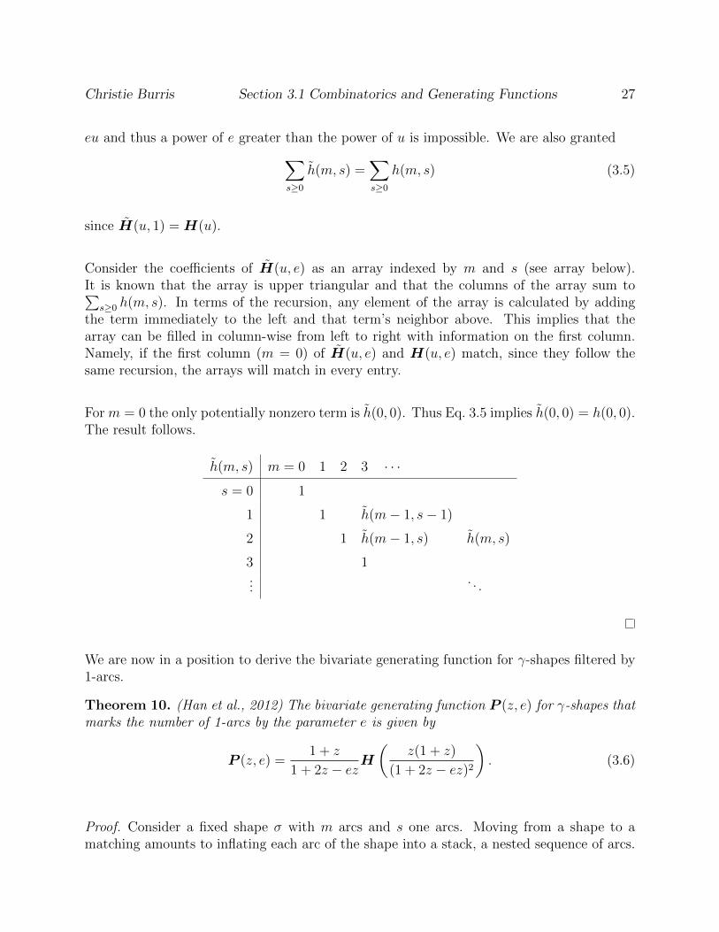
3.1 The (orange) arc is inflated. . . . . . . . . . . . . . . . . . . . . . . . . . . . 22
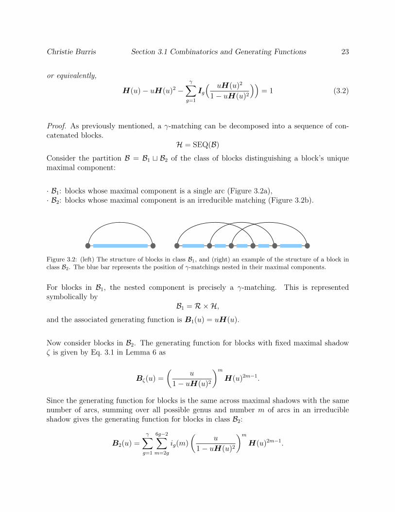
3.2 (left) The structure of blocks in class B1, and (right) an example of the struc-ture of a block in class B2. The blue bar represents the position of γ-matchingsnested in their maximal components. . . . . . . . . . . . . . . . . . . . . . . 23
3.3 Irreducible shadows of genus g = 1. . . . . . . . . . . . . . . . . . . . . . . . 31
A.1 An example of a ∆-domain, ∆(π/4, 2). . . . . . . . . . . . . . . . . . . . . . 58
v

List of Tables
3.1 Classes and generating functions associated with γ-structures . . . . . . . . . 21
4.1 Growth coefficients αγ for the expectation of the longest block in γ-structures,0 ≤ γ ≤ 3 . . . . . . . . . . . . . . . . . . . . . . . . . . . . . . . . . . . . . 56
vi
Chapter 1
Introduction
The central dogma of molecular biology has pervaded scientific literature since the 1950ssoon after Watson and Crick proposed the double helix structure of DNA, both of whomare predominantly responsible for its inception [3]. In essence, the central dogma states thatgenetic information is passed from DNA to messenger RNA (mRNA) which in turn trans-late into amino acids that assemble into proteins [24]. This simplified narrative has beenquestioned in recent years after the realization that only 1.5% of the human genome codesfor proteins [14]. What then is the role of the other 98% of non-coding RNA (ncRNA)?The initial inclination to follow the central dogma that led to the term ”junk” DNA even-tually dissipated. Researchers are now aware of numerous regulatory functions carried outby ncRNA [16].
The major distinction between DNA and RNA, apart from their respective nucleotide compo-sitions is the nature of the nucleotide pairings. A sequence and its set of pairings is referredto as a secondary structure. Similarly, a molecule’s tertiary structure additionally makesreference to its spatial embedding. For instance, DNA is double-stranded; the well-knowndouble helix tertiary structure is formed by two single strands held together by nucleotidespaired laterally. RNA however is single stranded, to mean that its nucleotides are pairedwith one another. As a result, the set of RNA secondary structures appearing in natureis diverse in shape. In recent years it has been shown that the structure of RNA plays animportant role in its function, likened to a lock and key system [8,16].
The current state of technology is such that gathering structural information is substantiallymore expensive and time consuming than gathering sequential information. As such, manyresearchers have turned to modeling structures constrained by laws of thermodynamics inan effort to supplement experimental data. The software used to implement these modelsand the subsequent analysis is continuously being updated and optimized for efficiency andbiological accuracy [22]. Much of this work is centered around identifying ways to reduce
1
Christie Burris Chapter 1. Introduction 2
the complexity of a given model.
Laws of biophysics provide the framework for sampling structures from sequences. Looselyspeaking, the minimum free energy (mfe) of an RNA molecule is the amount of energy re-quired to unpair its nucleotide chain; the lower the energy, the more energy is required tobreak apart the bonds. Thus it is reasonable to assume that a stable RNA structure ap-pearing in nature is one that attains its mfe. Dynamic programming algorithms are used toapproximate the minimum free energy for RNA molecules [8].
Numerous polynomial-time algorithms exist for predicting RNA secondary structures. How-ever, the prediction of pseudoknot structures is NP-complete. Methods for increasing theefficiency of these algorithms rely on the assumption that certain matrices in dynamic pro-gramming routines are sparse [15]. Mohl et al. in [17] and Huang and Reidys in [13] studysparcification of pseudoknots in an effort to lower space requirements. One property thatimplies sparsity is the polymer-zeta property which asserts that two nucleotides of distancem form a base pair with probability bm−c for some constants b > 0, c > 1. If this propertyholds, long-distance base pairs have low probability.
Another important property that characterizes RNA sequences is their 5’-3’ distance. Amolecule has a so-called direction indicated by the asymmetry at the ends of a strand. The5’-3’ distance is defined as the length of the shortest path traversed along paired nucleotidesfrom the 5’ end to the 3’ end of the molecule. As such, this distance is considered a measureof ’circularization’, an important phenomenon amongst viral and messenger RNA. Yoffe et.al in [25] shows that the 5’-3’ distance of RNA molecules is necessarily small, and largelyindependent of their length and sequence. The results of [11] show that the 5’-3’ distancesof random RNA secondary structures are distinctively smaller than those of biological RNAmolecules and mfe structures.
The purpose of this paper and others is to investigate the spectrum of the lengths betweenpaired nucleotides as it relates to the 5’-3’ distance and the polymer-zeta property. Whatfollows is a combinatorial construction of RNA structures that lends itself well to asymptoticanalysis of object parameters. Section 2 provides the relevant definitions and theorems tocarry out the transfer from biological information to mathematical information. Section 3provides the main result of this paper, the expected value of the length of certain irreduciblecomponents related to nucleotide pairings.
Chapter 2
Background
2.1 RNA Structures
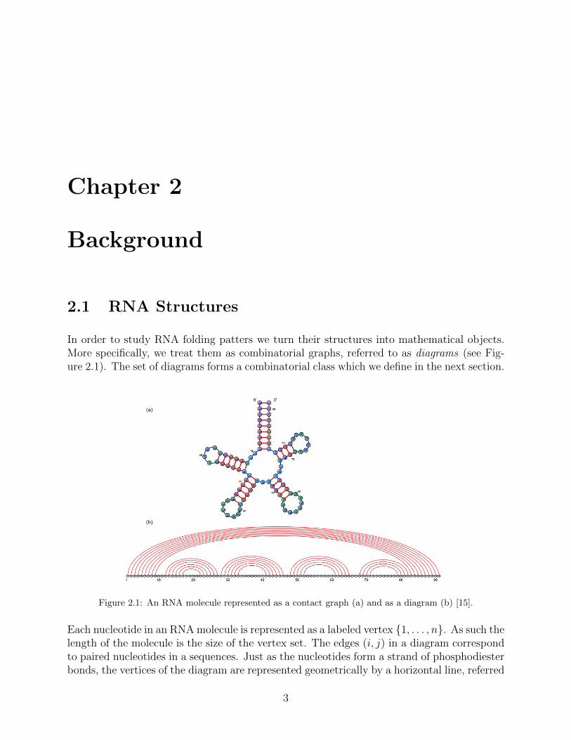
In order to study RNA folding patters we turn their structures into mathematical objects.More specifically, we treat them as combinatorial graphs, referred to as diagrams (see Fig-ure 2.1). The set of diagrams forms a combinatorial class which we define in the next section.
Figure 2.1: An RNA molecule represented as a contact graph (a) and as a diagram (b) [15].
Each nucleotide in an RNA molecule is represented as a labeled vertex 1, . . . , n. As such thelength of the molecule is the size of the vertex set. The edges (i, j) in a diagram correspondto paired nucleotides in a sequences. Just as the nucleotides form a strand of phosphodiesterbonds, the vertices of the diagram are represented geometrically by a horizontal line, referred
3

Christie Burris Section 2.1 RNA Structures 4
to as a backbone, which consists of the vertices 1, . . . , n and distinguished edges i, i + 1for all 1 ≤ i ≤ n − 1. Additional pairings are represented as arcs in the upper half-plane,including non-phosphodiester bonds (i, i + 1) which we refer to as 1-arcs. The length of anarc (i, j) is given by j − i.
Notice that the RNA structure in Figure 2.1 transfers to a diagram with no crossing arcs.This notion of crossing is essential to the mathematical and computational study of RNAstructures.
Definition 1. Two arcs (i, j) and (i′, j′) are crossing if i < i′ < j < j′.
Definition 2. An RNA secondary structure is a molecule whose corresponding diagramsatisfies the following conditions.
1. non-existence of 1-arcs : if (i, j) is an arc, then j − i ≥ 2.
2. non-existence of base triples : any two arcs do not share a common vertex.
3. non-existence of crossing arcs : any two arcs (i, j) and (i′, j′) are noncrossing, i.e. eitheri < j < i′ < j′ or i′ < j′ < i < j.
Namely, an RNA structure S is contained in the class S if and only if the above conditionsare held.
Definition 3. A stack of length τ is a maximal sequence of τ parallel arcs,((i, j), (i+1, j−1),
(i+2, j−2), . . . (i+τ, j−τ)). Further, an RNA structure S is τ -canonical if it has minimum
stack-length τ .
Remark. Stacks of length one are energetically unstable. Stacks of at least 2 or 3 aretypically found in biological structures. The generating functions defined in later sectionsfilter by minimum arc and stack length.
Definition 4. An arc in a diagram is considered a rainbow if it is maximal with respect tothe partial order (i, j) ≤ (i′, j′) ⇐⇒ i′ ≤ i < j ≤ j′.
Definition 5. A diagram with no crossing arcs is irreducible if it contains a rainbow con-necting the first and last vertex.
In order for graphs to lend themselves nicely to the type of analysis performed in this paper,the class of diagrams must be realized as a combination of three combinatorial operators onfundamental combinatorial objects.
i. A = B + C.
ii. A = B × C.

Christie Burris Section 2.1 RNA Structures 5
iii. A = SEQ(B).
(i) refers to the union of classes, (ii) to the Cartesian product of classes and (iii) to the unionof Cartesian products Bn for all n > 0.
We go into further detail on this construction later. However we note here that if a combi-natorial class, in this case the class of RNA structures of a particular kind, can be realizedas a combination of these three operators, then the transfer from combinatorial objects togenerating functions can be carried out in a fairly simple way. This transfer is referred to asthe symbolic transfer or symbolic enumeration.
The class of RNA structures with no restriction on crossing arcs poses a challenge as thestructures do not clearly contain irreducible substructures of a fundamental kind. By funda-mental we mean structures with polynomial generating functions filtered by arcs or vertices.However, there are meaningful subclasses that allow for crossing in such a way that they canbe constructed via symbolic enumeration.
One way to filter pseudoknot diagrams is by topological genus, which was first proposedin [19] and studied further in [23]. Topological objects hold combinatorial information in theform of key invariants that in turn provide information on the structure of the underlyinggraph. The idea is to pass from an drawing of a structure in R2 to a surface that admitsan embedding — a drawing without crossings. From this notion of embedding on a higherdimensional surface, one defines the genus of a diagram as the minimal integer g such thatthe graph can be embedded on a surface of genus g. By definition, secondary structures areplanar graphs of genus 0 since they are drawn in R2 without crossings.
The particular type of graph embedding employed in this treatment of pseudoknot structuresis called a combinatorial embedding — an embedding that uniquely defines cyclic orderingsof edges incident to each vertex. Consequently, the boundary components of an embeddingare defined as the natural cyclic orders of the edges. In our case, this notion is straightforward since each edge is seen exactly once when traversing the boundaries. Combinatorialembeddings encode diagrams onto closed, orientable surfaces.
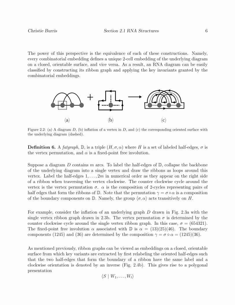
A combinatorial embedding is commonly represented by a fatgraph, or ribbon graph — atopological surface formed by a series of “fattenings” of the underlying diagram. Namely,vertices are inflated to discs and edges are inflated to ribbons with two boundaries referredto as half-edges (see Fig. 2.2). Associated with each vertex is a cyclic ordering of the half-edges. The resulting object is an oriented surface with boundary such that the half-edgesthat form the boundary of a ribbon are oriented in opposite directions (Fig. 2.2c). A moreformal definition involving permutations is given below.
Christie Burris Section 2.1 RNA Structures 6
The power of this perspective is the equivalence of each of these constructions. Namely,every combinatorial embedding defines a unique 2-cell embedding of the underlying diagramon a closed, orientable surface, and vice versa. As a result, an RNA diagram can be easilyclassified by constructing its ribbon graph and applying the key invariants granted by thecombinatorial embeddings.
+
(a) (b) (c)
Figure 2.2: (a) A diagram D, (b) inflation of a vertex in D, and (c) the corresponding oriented surface withthe underlying diagram (dashed).
Definition 6. A fatgraph, D, is a triple (H, σ, α) where H is a set of labeled half-edges, σ isthe vertex permutation, and α is a fixed-point free involution.
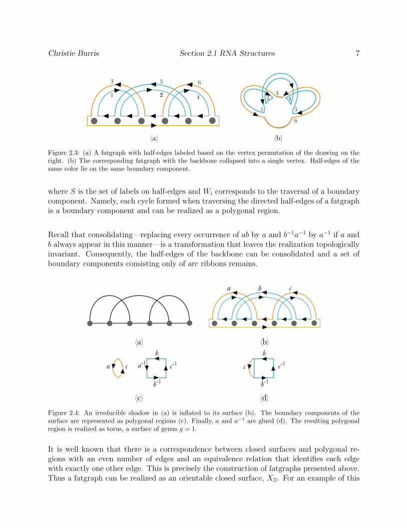
Suppose a diagram D contains m arcs. To label the half-edges of D, collapse the backboneof the underlying diagram into a single vertex and draw the ribbons as loops around thisvertex. Label the half-edges 1, . . . , 2m in numerical order as they appear on the right sideof a ribbon when traversing the vertex clockwise. The counter clockwise cycle around thevertex is the vertex permutation σ. α is the composition of 2-cycles representing pairs ofhalf edges that form the ribbons of D. Note that the permutation γ = σ α is a compositionof the boundary components on D. Namely, the group 〈σ, α〉 acts transitively on H.
For example, consider the inflation of an underlying graph D drawn in Fig. 2.3a with thesingle vertex ribbon graph drawn in 2.3b. The vertex permutation σ is determined by thecounter clockwise cycle around the single vertex ribbon graph. In this case, σ = (654321).The fixed-point free involution α associated with D is α = (13)(25)(46). The boundarycomponents (1245) and (36) are determined by the composition γ = σ α = (1245)(36).
As mentioned previously, ribbon graphs can be viewed as embeddings on a closed, orientablesurface from which key variants are extracted by first relabeling the oriented half-edges suchthat the two half-edges that form the boundary of a ribbon have the same label and aclockwise orientation is denoted by an inverse (Fig. 2.4b). This gives rise to a polygonalpresentation
〈S | W1, . . . ,Wl〉
Christie Burris Section 2.1 RNA Structures 7
1
23
4
5
6
1
3 5
2
6
2 4
(a) (b)
Figure 2.3: (a) A fatgraph with half-edges labeled based on the vertex permutation of the drawing on theright. (b) The corresponding fatgraph with the backbone collapsed into a single vertex. Half-edges of thesame color lie on the same boundary component.
where S is the set of labels on half-edges and Wi corresponds to the traversal of a boundarycomponent. Namely, each cycle formed when traversing the directed half-edges of a fatgraphis a boundary component and can be realized as a polygonal region.
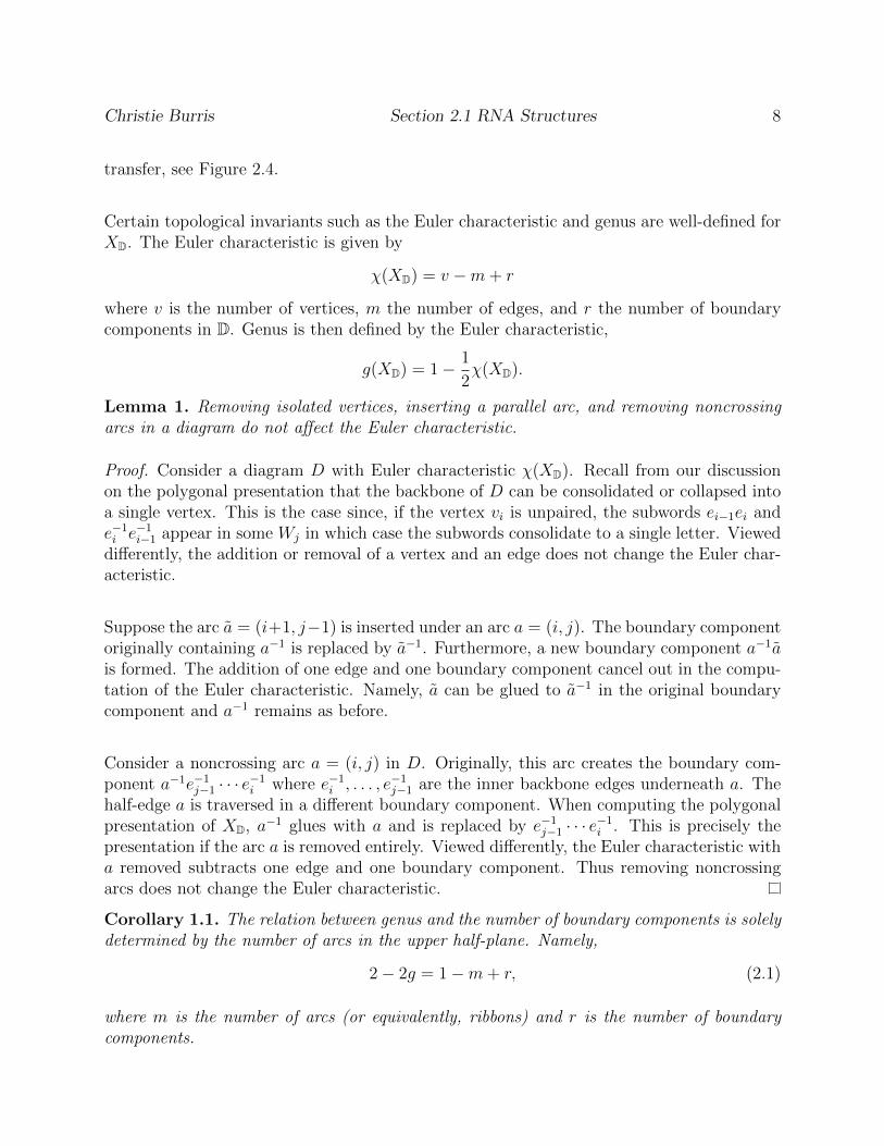
Recall that consolidating—replacing every occurrence of ab by a and b−1a−1 by a−1 if a andb always appear in this manner—is a transformation that leaves the realization topologicallyinvariant. Consequently, the half-edges of the backbone can be consolidated and a set ofboundary components consisting only of arc ribbons remains.
(a) (b)
(c) (d)
a b c
a c a-1
c-1
b-1
b
c c-1
b-1
b
Figure 2.4: An irreducible shadow in (a) is inflated to its surface (b). The boundary components of thesurface are represented as polygonal regions (c). Finally, a and a−1 are glued (d). The resulting polygonalregion is realized as torus, a surface of genus g = 1.
It is well known that there is a correspondence between closed surfaces and polygonal re-gions with an even number of edges and an equivalence relation that identifies each edgewith exactly one other edge. This is precisely the construction of fatgraphs presented above.Thus a fatgraph can be realized as an orientable closed surface, XD. For an example of this
Christie Burris Section 2.1 RNA Structures 8
transfer, see Figure 2.4.
Certain topological invariants such as the Euler characteristic and genus are well-defined forXD. The Euler characteristic is given by
χ(XD) = v −m+ r
where v is the number of vertices, m the number of edges, and r the number of boundarycomponents in D. Genus is then defined by the Euler characteristic,
g(XD) = 1− 1
2χ(XD).
Lemma 1. Removing isolated vertices, inserting a parallel arc, and removing noncrossingarcs in a diagram do not affect the Euler characteristic.
Proof. Consider a diagram D with Euler characteristic χ(XD). Recall from our discussionon the polygonal presentation that the backbone of D can be consolidated or collapsed intoa single vertex. This is the case since, if the vertex vi is unpaired, the subwords ei−1ei ande−1i e−1
i−1 appear in some Wj in which case the subwords consolidate to a single letter. Vieweddifferently, the addition or removal of a vertex and an edge does not change the Euler char-acteristic.
Suppose the arc a = (i+1, j−1) is inserted under an arc a = (i, j). The boundary componentoriginally containing a−1 is replaced by a−1. Furthermore, a new boundary component a−1ais formed. The addition of one edge and one boundary component cancel out in the compu-tation of the Euler characteristic. Namely, a can be glued to a−1 in the original boundarycomponent and a−1 remains as before.
Consider a noncrossing arc a = (i, j) in D. Originally, this arc creates the boundary com-ponent a−1e−1
j−1 · · · e−1i where e−1
i , . . . , e−1j−1 are the inner backbone edges underneath a. The
half-edge a is traversed in a different boundary component. When computing the polygonalpresentation of XD, a−1 glues with a and is replaced by e−1
j−1 · · · e−1i . This is precisely the
presentation if the arc a is removed entirely. Viewed differently, the Euler characteristic witha removed subtracts one edge and one boundary component. Thus removing noncrossingarcs does not change the Euler characteristic.
Corollary 1.1. The relation between genus and the number of boundary components is solelydetermined by the number of arcs in the upper half-plane. Namely,
2− 2g = 1−m+ r, (2.1)
where m is the number of arcs (or equivalently, ribbons) and r is the number of boundarycomponents.
Christie Burris Section 2.1 RNA Structures 9
Remark. Corollary 1.1 offers a means of computing the genus of a diagram with minimaleffort. Namely, a diagram is fattened and the half-edges are traversed to compute thenumber of boundary components. This information along with the number of arcs is all thatis required to compute the genus. For simple diagrams this process can be carried out byhand. However, given an arbitrary graph G, it is NP-complete to find the smallest g suchthat G has a combinatorial embedding on a genus-g surface [21].
The genus of ribbon graphs is used to classify subsets of pseudoknot structures. One naturalsubclass is the set of structures with fixed genus [7]. Another subclass that lends itself well torandom sampling is the set of k-noncrossing structures, studied in [2,20]. 10 other subclassesare collected in [18].
Section 3 analyzes the subclass known as γ-structures. For fixed γ, a γ-structure is composedof irreducible components (of a more general form than irreducibility defined above) whoseindividual genus is bounded by γ and contain no bonds of length one (1-arcs). Note thatthe genus of a particular structure is not bounded since the genus of a composition of nestedstructures is additive.
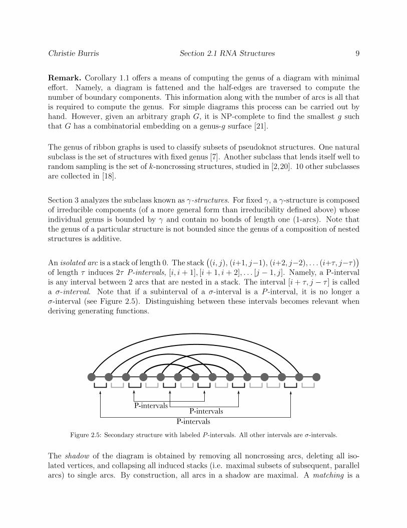
An isolated arc is a stack of length 0. The stack((i, j), (i+1, j−1), (i+2, j−2), . . . (i+τ, j−τ)
)of length τ induces 2τ P-intervals, [i, i + 1], [i + 1, i + 2], . . . [j − 1, j]. Namely, a P-intervalis any interval between 2 arcs that are nested in a stack. The interval [i+ τ, j − τ ] is calleda σ-interval. Note that if a subinterval of a σ-interval is a P -interval, it is no longer aσ-interval (see Figure 2.5). Distinguishing between these intervals becomes relevant whenderiving generating functions.
P-intervalsP-intervals
P-intervals
Figure 2.5: Secondary structure with labeled P -intervals. All other intervals are σ-intervals.
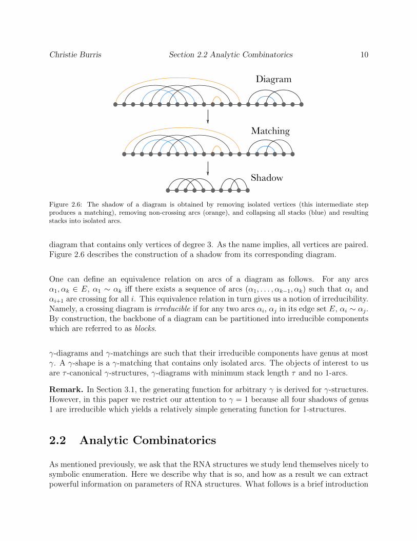
The shadow of the diagram is obtained by removing all noncrossing arcs, deleting all iso-lated vertices, and collapsing all induced stacks (i.e. maximal subsets of subsequent, parallelarcs) to single arcs. By construction, all arcs in a shadow are maximal. A matching is a
Christie Burris Section 2.2 Analytic Combinatorics 10
Diagram
Shadow
Matching
Figure 2.6: The shadow of a diagram is obtained by removing isolated vertices (this intermediate stepproduces a matching), removing non-crossing arcs (orange), and collapsing all stacks (blue) and resultingstacks into isolated arcs.
diagram that contains only vertices of degree 3. As the name implies, all vertices are paired.Figure 2.6 describes the construction of a shadow from its corresponding diagram.
One can define an equivalence relation on arcs of a diagram as follows. For any arcsα1, αk ∈ E, α1 ∼ αk iff there exists a sequence of arcs (α1, . . . , αk−1, αk) such that αi andαi+1 are crossing for all i. This equivalence relation in turn gives us a notion of irreducibility.Namely, a crossing diagram is irreducible if for any two arcs αi, αj in its edge set E, αi ∼ αj.By construction, the backbone of a diagram can be partitioned into irreducible componentswhich are referred to as blocks.
γ-diagrams and γ-matchings are such that their irreducible components have genus at mostγ. A γ-shape is a γ-matching that contains only isolated arcs. The objects of interest to usare τ -canonical γ-structures, γ-diagrams with minimum stack length τ and no 1-arcs.
Remark. In Section 3.1, the generating function for arbitrary γ is derived for γ-structures.However, in this paper we restrict our attention to γ = 1 because all four shadows of genus1 are irreducible which yields a relatively simple generating function for 1-structures.
2.2 Analytic Combinatorics
As mentioned previously, we ask that the RNA structures we study lend themselves nicely tosymbolic enumeration. Here we describe why that is so, and how as a result we can extractpowerful information on parameters of RNA structures. What follows is a brief introduction
Christie Burris Section 2.2 Analytic Combinatorics 11
to the field of Analytic Combinatorics, taken from Flajolet and Sedgewick [6], as it appliesto the analysis of RNA graph parameters. Throughout this section and the rest of the pa-per, we refer to definitions and theorem from [6] followed by their corresponding chapter orpage number. The work of many, including Li and Reidys in [15], and the generalization inSection 3 apply the framework provided in [6].
Analytic Combinatorics is the study of large combinatorial objects. For any field of mathe-matics, one can identify the objects and operators with which the field is concerned. Herethe objects of study are generating functions, formal power series whose coefficients carryinformation on a parameter of a combinatorial class. The operators are symbolic and ana-lytic transfers.
Symbolic transfers allow us to pass from combinatorial constructions to generating functionswithout the cumbersome task of solving a recurrence relation.
Definition 7. A combinatorial class, C, is a finite or denumerable set on which a size functionw : C → Z≥0 is defined such that the number of elements of any given size is finite. Of noteare two classes: the class containing one object of size 0, denoted E , and the class containingone object of size 1, denoted Z.
Three common constructions arise in the describing classes of RNA structures.
A = B t C
refers to A as the disjoint union of classes B and C. Similarly,
A = B × C
if the elements of A can be realized as the ordered pair of an object from B and an objectfrom C. The size of a pair a = (b, c) is computed w(a) = w(b) + w(c). Finally, the sequenceclass
A = SEQ(B)
is the infinite union of the classes B, B × B, etc. together with the empty class E . Namely,
SEQ(B) = E +∑n≥1
Bn
The size of an object a = (b1, b2, . . . , bj) is w(a) = w(b1) + w(b2) + · · · + w(bj). Note thatthis definition of size is well-defined only if B contains no empty word.
Christie Burris Section 2.2 Analytic Combinatorics 12
The symbolic transfer can be summarized by the following dictionary from combinatorialclass to generating function.
E =⇒ E(z) = 1
Z =⇒ Z(z) = z
A = B t C =⇒ A(z) = B(z) + C(z)
A = B × C =⇒ A(z) = B(z) ·C(z)
A = SEQ(B) =⇒ A(z) = 11−B(z)
The last transfer holds only when B does not contain an empty structure. To see this,consider
A = SEQ(B) = ε t B t (B × B) t · · ·
where ε is the null object. By the first two transfers,
A(z) = 1 + B(z) + B(z)2 + · · · =∑i≥0
(B(z))i .
Loosely speaking, the sum can be realized as a geometric series and the transfer seems ob-vious. However this representation of the geometric series is usually followed by a bound onB(z) in accordance with the notion of convergence which is only valid if the objects underscrutiny are analytic objects. Here the objects are formal power series with coefficients inthe ring Q. One arrives at the equation in the transfer by considering the notion of inversesin the ring Q[[x]]. The transfer holds if and only if 1−B(z) has an inverse in Q[[x]]. Namely,if 1−B(z) has a nonzero constant term, hence the reason why B must not contain an emptystructure.
The analytic transfer allows us to pass from analytic functions (realized as convergent powerseries) to coefficient asymptotics. How then do we arrive at an analytic function when theoriginal generating functions are formal objects? If it is possible to extract a functionalequation whose solution is the generating function, then considering the equation as ananalytic function allows us to pass to coefficient asymptotics. The guiding principles of thistransfer are the following, taken from [6].
1. The location of a function’s singularities dictates the exponential growth of its coeffi-cients.
2. The nature of a function’s singularities determines the associate subexponential factor.
The first principle is an immediate consequence of the definition of power series convergence.The second principle is the topic of Chapter 6 in [6]. Moreover, there is a correspondencebetween the asymptotic expansion of a function near its dominant singularities and the
Christie Burris Section 2.2 Analytic Combinatorics 13
asymptotic expansion of the function’s coefficients. See the appendix for a closer look at thedefinitions behind this framework. Below are two examples of analytic transfer.
f(z) = 1
1−(z/ρ)=⇒ [zn]f(z) = ρ−n
f(z) = 1(1−(z/ρ))α
=⇒ [zn]f(z) ≈ nα−1
Γ(α)ρ−n (α ∈ C\Z≤0)
The first is a well-known transfer of the geometric series. The second transfer is key for theanalysis of RNA structures. We state the transfer as a theorem to refer back to in Section 3.A proof sketch can be found in the appendix.
Theorem 2. (Flajolet, Sedgewick) Let α be an arbitrary complex number in C\Z≤0. Thecoefficient of zn in
f(z) = (1− z)−α
admits for large n a complete asymptotic expansion in descending powers of n,
[zn]f(z) ∼ nα−1
Γ(α)(1 +O(n−1)).
A similar theorem vital to the transfer from generating function to asymptotic estimation ofcoefficients involves Big-Oh and little-oh.
Theorem 3. (Flajolet, Sedgewick) Let α, β ∈ R and let f(z) be a function that is ∆-analytic.
(i) Assume that f(z) satisfies in the intersection of a neighborhood of 1 with its ∆-domainthe condition
f(z) = O((1− z)−α).
Then one has:[zn]f(z) = O(nα−1).
(ii) Assume that f(z) satisfies in the intersection of a neighborhood of 1 with its ∆-domainthe condition
f(z) = o((1− z)−α).
Then one has:[zn]f(z) = o(nα−1).
Recall that we have shifted from viewing generating functions as formal objects to analyticobjects. Via symbolic enumeration one can derive a functional form for a generating func-tion. Treating the functional form as a complex function in one (or more) variables one can

Christie Burris Section 2.2 Analytic Combinatorics 14
then seek its asymptotic expansion near its dominant singularity, a process referred to assingularity analysis. By Theorems 2 and 3 one can carry out a term-by-term transfer of theasymptotic expansion to arrive at an asymptotic estimate of the coefficients.
It is also possible that an explicit functional form for the generating function can not befound, or rather need not be found. This is the case in Section 3 for γ-matchings. Theorem 4gives an alternative to carrying out explicit singularity analysis given an implicit formula forthe generating function. Namely, the generating function y(z) satisfies y(z) = F (z, y).
Theorem 4. (Flajolet, Sedgewick) Let F (z, w) be a bivariate function analytic at (z, w) =(z0, w0). Assume the conditions:
F (z0, w0) = 0, Fz(z0, w0) 6= 0, Fw(z0, w0) = 0, Fww(z0, w0) 6= 0
Choose an arbitrary ray angle θ emanating from z0. Then there exists a neighborhood Ω ofz0 such that at every point z of Ω with z 6= z0 and z not on the ray, the equation F (z, y) = 0admits two analytic solutions y1(z) and y2(z) that satisfy, as z → z0:
y1(z) = y0 + δ√
1− z/z0 +O(1− z/z0), δ :=
√2z0Fz(z0, w0)
Fww(z0, w0)
and similarly for y2 whose expansion is obtained by changing the square root to a negativesquare root.
Remark. Theorem 4 demonstrates the universality of the square-root singularity type.Combinatorial classes that are defined by symbolic enumeration of subclasses with finitegenerating functions admit a recursion as well as a generating function with an implicitfunctional form. The Analytic Implicit Function Theorem (AIFT) asserts that F (z, w) suf-ficiently smooth admits a unique solution
F (z, f(z)) = 0, |z| < ρ
where f(z) is analytic in the neighborhood |z| < ρ. Locally, near (ρ, f(ρ)), F (z, w) has aTaylor expansion
F + (w − f(ρ))Fw + (z − ρ)Fz +1
2(w − f(ρ))2Fww,
(lower order terms omitted). The assumption F = Fw = 0 of AIFT simlifes the aboveequation such that the solution to F (z, w) near z = ρ admits a square-root form.
Each of the three Theorems from [6] make statements regarding the asymptotic behavior ofthe coefficients of a function’s series expansion near its singularity. To arrive at the singular
Christie Burris Section 2.2 Analytic Combinatorics 15
expansion of our generating functions, we first investigate the nature of their singularities.i.e. locate their dominant singularity and determine uniqueness. To do so we employ Pring-sheim’s Theorem which is useful for our analysis since generating functions necessarily havenon-negative coefficients.
Theorem 5. (Pringsheim’s Theorem) If f(z) is representable at the origin by a series ex-pansion that has non-negative coefficients and radius of convergence R, then the point z = Ris a singularity of f(z).
Until now we have implicitly only considered generating functions of a single variable (OGFs)as they carry information on the size parameter. However, we are not restricted to asymptoticcoefficient analysis of OGFs. Analytic combinatorics also provides a framework that makesit easy to study properties of parameters of graphs such as: How many substructures of aparticular kind appear in a random graph? To answer this type of question, we introducethe bivariate generating function
F (z, u) =∑n,b
f(n, b)znub,
where f(n, b) is the count of the number of objects of size n with the additional property ofhaving b substructures of a particular kind.
We are still interested in extracting coefficient asymptotics from these bivariate generatingfunctions. However, a double coefficient extraction
fn,b = [znub]F (z, u)
is quite difficult. Instead, an equally powerful ”horizontal” extraction does the trick inproviding asymptotics that appear in moments. The goal becomes to estimate the horizontalgenerating function
fn(u) :=∑b
f(n, b)ub ≡ [zn]F (z, u)
as this term appears in the moment generating function which we discuss in the next section.
The method for studying fn(u) is known as perturbation analysis since F (z, 1) = F (z). Thevariable u marking the parameter of interest is regarded as inducing a deformation of theOGF. The way in which such deformations affect the type of singularity of the counting gen-erating functions can then be studied. It happens that the Hankel contours employed in thederivation of univariate asymptotic analysis have the additional nice property of producinguniform asymptotic expansions in the bivariate case. With uniformity of expansion, one canuniformly estimate fn(u) to mean that a small perturbation in u yields small perturbationsin fn(u). Namely, for u ∈ Nε(1),
fn(1) ≈ Cn−αρ−n =⇒ fn(u) ≈ C(u)n−α(u)ρ(u)−n. (2.2)
Christie Burris Section 2.3 Probabilistic Graph Theory 16
Definition 8. Let fu(s)u∈U be a family of functions indexed by U . The asymptoticequivalence
fu(s) = O(g(s)) (s→ s0),
is said to be uniform with respect to u if there exists an absolute constant K (independentof u ∈ U) and a fixed neighborhood N(s0) of s0 such that
∀u ∈ U, s ∈ N(s0) , |fu(s)| ≤ K|g(s)|.
An asymptotic expansion
fu(s) = h0(s) + h1(s) + . . .+O(hm(s))
where h0(s) >> h1(s) >> . . . >> hm(s) is uniform if for each m the Big-Oh error term isuniform.
What makes the method of analytic combinatorics so powerful is the universality of theschema that govern singularity analysis and transfer theorems. From simple derivations ofgenerating functions through symbolic enumeration, we are given objects that, while countingprofoundly distinct objects, have the same behavior near their dominant singularity, and thussimilar asymptotic behavior of their coefficients.
2.3 Probabilistic Graph Theory
As the name implies, probabilistic graph theory treats graph theoretic objects as probabilisticones to answer questions regarding how graphs with particular properties behave on average.A measure space, or a probability space (Ω,P) is the set of all possible graphs (given propertiesof interest) along with a σ-algebra A of subsets of Ω, endowed with a specified probabilityfunction P : Ω → [0, 1]. The σ-algebra (i) contains the empty set, and (ii) is closed undercomplements and countable unions. Additionally, P is additive over finite and countableunions of disjoint sets, and satisfies P(Ω) = 1.
We say an event A ⊂ Ω is a subset of Ω that occurs with probability
P(A) :=∑ω∈A
P(ω).
To illustrate this construction, suppose you are interested in a certain property of graphswith n vertices and no additional specified restrictions (these are spanning subgraphs of thecomplete graph on n vertices). Label the set of all such graphs Gn. You might choose toassociate to Gn the uniform probability function. Namely, for G ∈ Gn,
P(G) =1
|Gn|.
Christie Burris Section 2.3 Probabilistic Graph Theory 17
where |Gn| = 2(n2) since each graph is uniquely specified by whether or not each possibleedge–of which there are
(n2
)–appears.
Naturally, we wish to study how graphs look on average as the size of the graph grows with-out bound. A particular property of a graph, referred to as a parameter, can be studied bymeans of (discrete) random variables. A random variable X is a function from the samplespace Ω to the real numbers, or in the case of combinatorial classes, the non-negative inte-gers. In particular, to study the connectivity of a graph, the number of edges needed to beremoved in order to disconnect the graph, one can define a random variable which assigns toeach graph its connectivity number. Further analysis can provide insight into connectivityof graphs on average.
The event(X = m) = ω ∈ Ω : X(ω) = m
plays an important role in analyzing graph parameters. One can further define the eventsX < m, X ≤ m, X > m, and X ≥ m analogously.
The probability generating function (pgf) of a discrete random variable X with values in Z≥0,is defined as
p(u) :=∑b
P(X = b)ub.
The goal of this treatment as mentioned above is to determine whether a given combinatorialparameter holds on average as n becomes large. For this we introduce the following asymp-totic notation. Given a sequence of probability spaces (Ωn,Pn)n≥1 we say that propertyA is satisfied asymptotically almost surely (a.a.s.) if
Pn(An)→ 1, as n→∞
where An is the subset of graphs of size n satisfying property A. Similarly, for real valuedfunctions f, g : N→ R we say f ∼ g if
f(n)
g(n)→ 1, as n→∞.
One often considers satisfying property A as an event X = m where the random variableX indicates whether property A is satisfied. Xn can then be defined as the restriction ofX to the subspace of graphs of size n. The above-mentioned notions of random variables,sequences of probability spaces, and asymptotic behavior provide the objects and analyticframework for studying graphs. In the next section we define moments of a distribution of arandom variable, which we will see provide the quantification necessary to derive asymptotic
Christie Burris Section 2.3 Probabilistic Graph Theory 18
approximations.
In probability theory, expectation is the average value, or mean, of a random variable Xdenoted by E[X]. Variance V[X] quantifies the notion of how concentrated the randomvariable is around its expected value. Expectation and variance are also known as the firstand second moments of a distribution, respectively, and are defined below.
E[X] :=∑ω∈Ω
X(ω)P(ω)
V[X] := E[(X− E[X])2]
Variance is more often expressed in the expanded form which is possible by linearity ofexpectation.
V[X] = E[X2]− E2[X].
Markov’s Inequality provides an upper bound on the probability of an event by a ratio of theexpectation which yields a relationship between these two quantities. The proof is straight-forward from the definitions.
Markov’s Inequality. Let X be a nonnegative random variable and m a positive realnumber. Then
P(X ≥ m) ≤ E[X]
m.
Another important theorem and the one used in the following chapters is due to Markov’steacher Chebyshev. Chebyshev’s Inequality (eq. 2.3) provides an upper bound for the vari-ance of a random variable about its mean.
Chebyshev’s Inequality. Let X be a nonnegative random variable and m a positive realnumber. Then
P(∣∣X− E[X]
∣∣ ≥ m) ≤ V[X]
m2.
Another key feature in analytic combinatorics is convergence in distribution or convergencein law which provides the relationship between combinatorial parameters and asymptoticproperties. We say that a limit law exists for a parameter if there is convergence as ngrows of the corresponding family of cumulative distribution functions. In this case of RNAsecondary structures, the limit law is discrete to mean convergence is established withoutstandardizing the random variable.
Definition 9. The discrete random variables Xn supported by Z≥0 are said to converge inlaw to a discrete random variable Y supported by Z≥0, written Xn ⇒ Y if for each k ≥ 0,
limn→∞
P(Xn ≤ k) = P(Y ≤ k).
Christie Burris Section 2.3 Probabilistic Graph Theory 19
A nice feature of limit laws of the discrete kind is their equivalence to local limit laws. Thereexists a local limit law if, for each k ≥ 0,
limn→∞
P(Xn = k) = P(Y = k).
We use the framework outlined above to extract important information regarding the struc-ture of RNA secondary structures in the next section.

Chapter 3
γ-structures
We begin with a biological inquiry. Can we specify the length of irreducible components ofγ-structures? The set of γ-structures is translated to a combinatorial class where the objectsof study are now graphs with properties generalized from known binding blocks. Throughsymbolic enumeration, information on the combinatorial class is transfered to formal gener-ating functions. We are then in a position to extract coefficients of the generating functionswhich provide a count of these objects of a particular length. Again the objects of studyare transfered from generating functions, or more specifically formal power series, to com-plex analytic functions. Through singularity analysis we are able to compute asymptoticestimates of the coefficients. Finally, we employ techniques from probabilistic graph theoryto produce likelihood estimates to yield a more rich understanding of the behavior of theoriginal biological objects.
First, we construct the generating function for τ -canonical γ-structures. Next we use toolsfrom Analytic Combinatorics and Probabilistic Graph Theory to derive the mean and vari-ance for the length of the longest block. Further results on the length-spectrum and unique-ness follow.
3.1 Combinatorics and Generating Functions
The main result of this section is the generating function for γ-structures. The theorems canbe found in Han et al. [10], however the proofs differ slightly. Han et al. does not restrict γ tobe 1 and thus diverges from the work below to derive the generating function for irreducibleshadows using the generating function for matchings filtered by genus.
The process of deriving Gτ (z) for arbitrary γ begins with deriving the OGF for γ-matchings,
20
Christie Burris Section 3.1 Combinatorics and Generating Functions 21
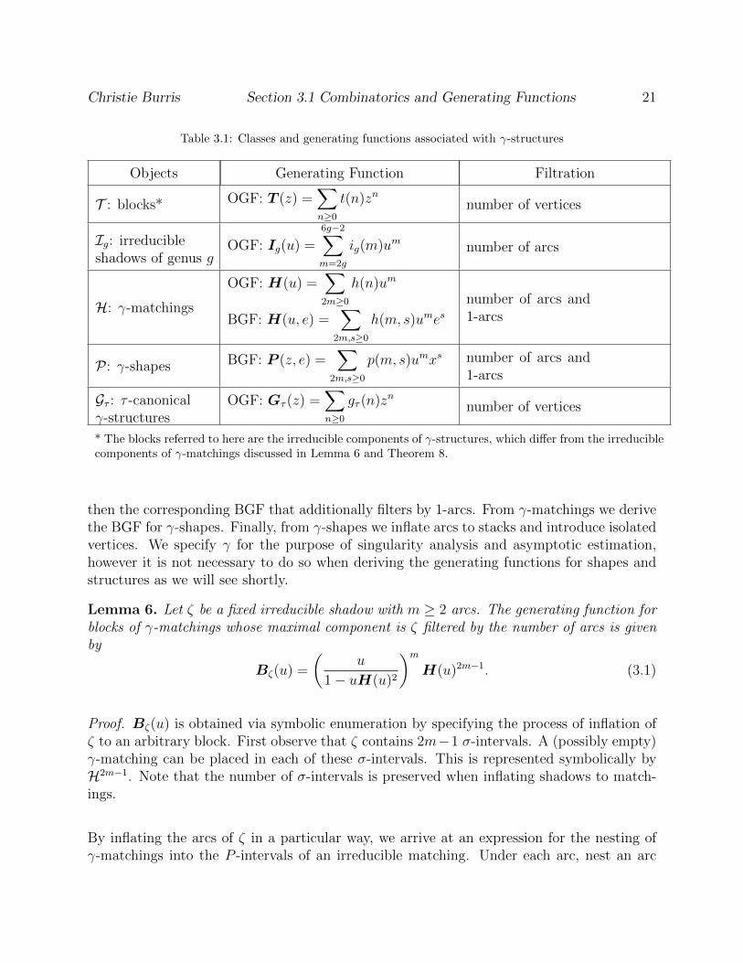
Table 3.1: Classes and generating functions associated with γ-structures
Objects Generating Function Filtration
T : blocks* OGF: T (z) =∑n≥0
t(n)zn number of vertices
Ig: irreducibleshadows of genus g
OGF: Ig(u) =
6g−2∑m=2g
ig(m)um number of arcs
H: γ-matchings
OGF: H(u) =∑
2m≥0
h(n)um
BGF: H(u, e) =∑
2m,s≥0
h(m, s)umesnumber of arcs and1-arcs
P : γ-shapes BGF: P (z, e) =∑
2m,s≥0
p(m, s)umxs number of arcs and1-arcs
Gτ : τ -canonicalγ-structures
OGF: Gτ (z) =∑n≥0
gτ (n)zn number of vertices
* The blocks referred to here are the irreducible components of γ-structures, which differ from the irreduciblecomponents of γ-matchings discussed in Lemma 6 and Theorem 8.
then the corresponding BGF that additionally filters by 1-arcs. From γ-matchings we derivethe BGF for γ-shapes. Finally, from γ-shapes we inflate arcs to stacks and introduce isolatedvertices. We specify γ for the purpose of singularity analysis and asymptotic estimation,however it is not necessary to do so when deriving the generating functions for shapes andstructures as we will see shortly.
Lemma 6. Let ζ be a fixed irreducible shadow with m ≥ 2 arcs. The generating function forblocks of γ-matchings whose maximal component is ζ filtered by the number of arcs is givenby
Bζ(u) =
(u
1− uH(u)2
)mH(u)2m−1. (3.1)
Proof. Bζ(u) is obtained via symbolic enumeration by specifying the process of inflation ofζ to an arbitrary block. First observe that ζ contains 2m−1 σ-intervals. A (possibly empty)γ-matching can be placed in each of these σ-intervals. This is represented symbolically byH2m−1. Note that the number of σ-intervals is preserved when inflating shadows to match-ings.
By inflating the arcs of ζ in a particular way, we arrive at an expression for the nesting ofγ-matchings into the P -intervals of an irreducible matching. Under each arc, nest an arc
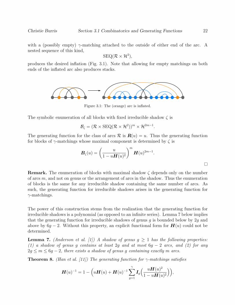
Christie Burris Section 3.1 Combinatorics and Generating Functions 22
with a (possibly empty) γ-matching attached to the outside of either end of the arc. Anested sequence of this kind,
SEQ(R×H2),
produces the desired inflation (Fig. 3.1). Note that allowing for empty matchings on bothends of the inflated arc also produces stacks.
Figure 3.1: The (orange) arc is inflated.
The symbolic enumeration of all blocks with fixed irreducible shadow ζ is
Bζ = (R× SEQ(R×H2))m ×H2m−1.
The generating function for the class of arcs R is R(u) = u. Thus the generating functionfor blocks of γ-matchings whose maximal component is determined by ζ is
Bζ(u) =
(u
1− uH(u)2
)mH(u)2m−1.
Remark. The enumeration of blocks with maximal shadow ζ depends only on the numberof arcs m, and not on genus or the arrangement of arcs in the shadow. Thus the enumerationof blocks is the same for any irreducible shadow containing the same number of arcs. Assuch, the generating function for irreducible shadows arises in the generating function forγ-matchings.
The power of this construction stems from the realization that the generating function forirreducible shadows is a polynomial (as opposed to an infinite series). Lemma 7 below impliesthat the generating function for irreducible shadows of genus g is bounded below by 2g andabove by 6g − 2. Without this property, an explicit functional form for H(u) could not bedetermined.
Lemma 7. (Anderson et al. [1]) A shadow of genus g ≥ 1 has the following properties:(1) a shadow of genus g contains at least 2g and at most 6g − 2 arcs, and (2) for any2g ≤ m ≤ 6g − 2, there exists a shadow of genus g containing exactly m arcs.
Theorem 8. (Han et al. [11]) The generating function for γ-matchings satisfies
H(u)−1 = 1−(uH(u) + H(u)−1
γ∑g=1
Ig
( uH(u)2
1− uH(u)2
)),
Christie Burris Section 3.1 Combinatorics and Generating Functions 23
or equivalently,
H(u)− uH(u)2 −γ∑g=1
Ig
( uH(u)2
1− uH(u)2
))= 1 (3.2)
Proof. As previously mentioned, a γ-matching can be decomposed into a sequence of con-catenated blocks.
H = SEQ(B)
Consider the partition B = B1 t B2 of the class of blocks distinguishing a block’s uniquemaximal component:
· B1: blocks whose maximal component is a single arc (Figure 3.2a),· B2: blocks whose maximal component is an irreducible matching (Figure 3.2b).
Figure 3.2: (left) The structure of blocks in class B1, and (right) an example of the structure of a block inclass B2. The blue bar represents the position of γ-matchings nested in their maximal components.
For blocks in B1, the nested component is precisely a γ-matching. This is representedsymbolically by
B1 = R×H,
and the associated generating function is B1(u) = uH(u).
Now consider blocks in B2. The generating function for blocks with fixed maximal shadowζ is given by Eq. 3.1 in Lemma 6 as
Bζ(u) =
(u
1− uH(u)2
)mH(u)2m−1.
Since the generating function for blocks is the same across maximal shadows with the samenumber of arcs, summing over all possible genus and number m of arcs in an irreducibleshadow gives the generating function for blocks in class B2:
B2(u) =
γ∑g=1
6g−2∑m=2g
ig(m)
(u
1− uH(u)2
)mH(u)2m−1.
Christie Burris Section 3.1 Combinatorics and Generating Functions 24
where ig(m) is the number of irreducible shadows with m arcs.
The empty diagram is taken to be a matching. Therefore [z0]H(u) = 1 and H(u) has aninverse in the ring of formal power series Q[[u]]. Since H = SEQ(B1 + B2), the generatingfunction for γ-matchings is
H(u)−1 = 1−(uH(u) +
γ∑g=1
6g−2∑m=2g
ig(m)
(u
1− uH(u)2
)mH(u)2m−1
)= 1−
(uH(u) + H(u)−1
γ∑g=1
6g−2∑m=2g
ig(m)
(uH(u)2
1− uH(u)2
)m )The generating function for irreducible shadows is
Ig(u) =
6g−2∑m=2g
ig(m)um.
Thus the inner sum in the generating function for γ-matchings can be realized as the com-position
Ig
(uH(u)2
1− uH(u)2
)=
6g−2∑m=2g
ig(m)
(uH(u)2
1− uH(u)2
)m.
This observation and the following algebraic manipulation takes us to the form of H(u)given in the statement of the theorem.
H(u)−1 = 1−(uH(u) + H(u)−1
γ∑g=1
6g−2∑m=2g
ig(m)
(uH(u)2
1− uH(u)2
)m )H(u)−1 = 1−
(uH(u) + H(u)−1
γ∑g=1
Ig
( uH(u)2
1− uH(u)2
))1 = H(u)−H(u)
(uH(u) + H(u)−1
γ∑g=1
Ig
( uH(u)2
1− uH(u)2
))1 = H(u)− uH(u)2 −
γ∑g=1
Ig
( uH(u)2
1− uH(u)2
))
Remark. Note that γ-matchings have no restriction on 1-arcs. Since γ-structures do notallow 1-arcs, it is necessary to identify all 1-arcs in a given γ-matching in order to ensurethey are eliminated during the inflation process. The following generating function for γ-matchings additionally filters by 1-arcs.
Christie Burris Section 3.1 Combinatorics and Generating Functions 25
Theorem 9. (Han et al., 2012) The bivariate generating function H(u, e) for γ-matchingsthat marks the number of 1-arcs by the parameter e is given by
H(u, e) =1
u+ 1− euH
(u
(u+ 1− eu)2
). (3.3)
Proof. We begin by defining a recursion for the number of γ-matchings with a labeled 1-arc.A PDE equivalent to this recursion is derived and a solution H(u, e) is determined. We thenshow that H(u, e) = H(u, e).
The number of γ-matching with m+ 1 arcs and s+ 1 1-arcs with one labeled 1-arc is
(s+ 1)h(m+ 1, s+ 1).
Each of these marked γ-matchings can be formed from γ-matching with m arcs by inserting(and marking) a 1-arc between any of the 2m − 1 adjacent pairs of vertices, or on eitherend of the sequence. Either the 1-arc is inserted underneath an existing 1-arc, or not. If itis inserted underneath an existing 1-arc, the resulting γ-matching has 1 additional arc andno additional 1-arcs since the inserted 1-arc replaces a 1-arc in the original structure. Theoriginal γ-matching has s+ 1 1-arcs, thus the number of places to insert the nested 1-arc iss+ 1. The count of such labeled γ-matchings is
(s+ 1)h(m, s+ 1).
Suppose the 1-arc is not inserted underneath an existing 1-arc. Then there are s original1-arcs and the number of possible insertion points is (2m + 1 − s). The resulting structurehas one additional arc contributing to the the count of arcs and 1-arcs. Then the count ofall such markings is
(2m+ 1− s)h(m, s).
Thus the recursion on γ-matchings with a labeled 1-arc is
(s+ 1)h(m+ 1, s+ 1) = (s+ 1)h(m, s+ 1) + (2m+ 1− s)h(m, s).
Notice that the terms in the recurrence relation resemble the coefficients of terms in thederivatives of H(u, e). Toward deriving a differential equation whose coefficients exactlymatch the recurrence relation at each m and s, consider the partial derivatives
∂
∂u
(H(u, e)
)=∑
2m,s≥0
mh(m, s)um−1es
∂
∂e
(H(u, e)
)=∑
2m,s≥0
sh(m, s)umes−1
Christie Burris Section 3.1 Combinatorics and Generating Functions 26
Extracting coefficients gives us
(s+ 1)h(m+ 1, s+ 1) = [um+1es]∂
∂e
(H(u, e)
)(s+ 1)h(m, s+ 1) = [umes]
∂
∂e
(H(u, e)
)mh(m, s) = [um−1es]
∂
∂u
(H(u, e)
)h(m, s) = [umes]H(u, e)
sh(m, s) = [umes−1]∂
∂e
(H(u, e)
)By shifting the coefficients we can extract the terms of the recurrence from the power um+1es,which in turn gives the PDE equivalent to the recurrence relation,
(1− u+ eu)∂
∂e
(H(u, e)
)= 2u2 ∂
∂u
(H(u, e)
)+ uH(u, e). (3.4)
Claim:
H(u, e) =1
u+ 1− euH
(u
(u+ 1− eu)2
)is a solution to (3.4) and H(u, e) = H(u, e).
First consider the partial derivatives of H(u, e). For ease of reading, label y = (u+1−eu)−2.
∂
∂u
(H(u, e)
)= (e− 1)yH(uy) + y2(eu− u+ 1)H ′(uy)
∂
∂e
(H(u, e)
)= uyH(uy) + 2(uy)2H ′(uy)
Plugging the potential solution into the PDE,
(1− u+ eu)(uyH + 2(uy)2H ′) = 2u2
((e− 1)yH + y2(eu− u+ 1)H ′)+
uH
u+ 1− eu
(1− u+ eu)uyH = 2u2(e− 1)yH +uH
u+ 1− eu(1− u+ eu)y = 2u(e− 1)y + 1.
The final equality holds by replacing y with its original form and equating the numeratorsof the left and right hand sides.
To prove that H(u, e) = H(u, e), we must show that h(m, s) = h(m, s) for all m, s ≥ 0.First note that for m > s, h(m, s) = 0—whenever e appears in H(u, e) it is in the product
Christie Burris Section 3.1 Combinatorics and Generating Functions 27
eu and thus a power of e greater than the power of u is impossible. We are also granted∑s≥0
h(m, s) =∑s≥0
h(m, s) (3.5)
since H(u, 1) = H(u).
Consider the coefficients of H(u, e) as an array indexed by m and s (see array below).It is known that the array is upper triangular and that the columns of the array sum to∑
s≥0 h(m, s). In terms of the recursion, any element of the array is calculated by addingthe term immediately to the left and that term’s neighbor above. This implies that thearray can be filled in column-wise from left to right with information on the first column.Namely, if the first column (m = 0) of H(u, e) and H(u, e) match, since they follow thesame recursion, the arrays will match in every entry.
For m = 0 the only potentially nonzero term is h(0, 0). Thus Eq. 3.5 implies h(0, 0) = h(0, 0).The result follows.
h(m, s) m = 0 1 2 3 · · ·
s = 0 1
1 1 h(m− 1, s− 1)
2 1 h(m− 1, s) h(m, s)
3 1...
. . .
We are now in a position to derive the bivariate generating function for γ-shapes filtered by1-arcs.
Theorem 10. (Han et al., 2012) The bivariate generating function P (z, e) for γ-shapes thatmarks the number of 1-arcs by the parameter e is given by
P (z, e) =1 + z
1 + 2z − ezH
(z(1 + z)
(1 + 2z − ez)2
). (3.6)
Proof. Consider a fixed shape σ with m arcs and s one arcs. Moving from a shape to amatching amounts to inflating each arc of the shape into a stack, a nested sequence of arcs.
Christie Burris Section 3.1 Combinatorics and Generating Functions 28
Since inflation preserves 1-arcs, the number of γ-matchings with shape σ is
Hσ(u, e) =
(u
1− u
)mes.
The generating function for γ-matchings can be rewritten
H(u, e) =∑s≥0
∑σ∈P(s)
Hσ(u, e) =∑m≥0
∑s≥0
p(m, s)
(u
1− u
)mes.
ForP (z, e) =
∑m≥0
∑s≥0
p(m, s)zmes,
the change of variable z = u1−u produces the equality
P (z, e) = H( z
1 + z, e)
=1 + z
1 + 2z − ezH
(z(1 + z)
(1 + 2z − ez)2
).
Lemma 11. (Han et al., 2012) Let σ be a fixed γ-shape with m ≥ 1 arcs and s ≥ 0 1-arcs.The bivariate generating function for τ -canonical γ-structures that have shape σ is given by
Gστ (z) =
1
1− z
(z2τ
(1− z2)(1− z)2 − (2z − z2)z2τ
)mzs. (3.7)
Proof. Recall that γ-structures do not contain 1-arcs, but possibly contain isolated vertices.To be τ -canonical is to have a minimum stack length τ . The proof follows a construc-tion similar to γ-matching wherein we considered inflation of arcs of irreducible shadowsin a particular way. Here we introduce the notion of induced arcs again, however the ob-jects concatenated to the arc are sequences of isolated vertices and lie inside the arc. Toavoid overcounting, we require that at least one of the two sequences of isolated vertices isnonempty.
Consider a fixed shadow σ with m arcs and s 1-arcs. To arrive at a τ -canonical γ-structureone inflates each arc by stacking induced arcs on top of the original arc, then inflates eachof the resulting arcs to a stack, and inserts isolated vertices underneath the original arcs.
The generating function for the class of vertices Z and arcs R are Z(z) = z and R(z) = z2,and a sequence of isolated vertices is represented symbolically and in a generating functionby
L = SEQ(Z), L(z) =1
1− z,
Christie Burris Section 3.1 Combinatorics and Generating Functions 29
respectively. Thus an induced arc is represented by
N = (R×L+R×L+R×L2)
The generating function for a nested sequence of induced arcs lying above an original arc is
z2
(1−
(z2 z
1− z+ z2 z
1− z+ z2
( z
1− z
)2))−1
(3.8)
Next, each arc in the induced stack is inflated to a τ -canonical stack. Eq. 3.8 is thentransformed into
z2τ
1− z2
(1− z2τ
1− z2
( z
1− z+
z
1− z+( z
1− z
)2))−1
(3.9)
Finally, sequences of isolated vertices are inserted between any two sets of original verticesplus the two endpoints. There are 2m− 1 pairs of adjacent vertices, s of which correspondto 1-arcs. Sequences nested under 1-arcs cannot be empty to ensure no 1-arcs appear in thefinal structure. The corresponding generating function for these inserted sequences is(
1
1− z
)2m+1−s(z
1− z
)s= zs
1
1− z
(1
1− z
)2m
(3.10)
Combining Eqs. 3.9 and 3.10, we arrive at the generating function for a τ -canonical γ-structures with fixed shape σ is
Gστ (z) = zs
1
1− z
(1
1− z
)2m(
z2τ
1− z2
(1− z2τ
1− z2
( z
1− z+
z
1− z+( z
1− z
)2))−1)m
(3.11)
The following algebraic manipulation gives us Eq. 3.11. In order to preserve readability, weonly do computation on the two rightmost terms of the product since the first two correspondto terms in Eq. 3.7.(
1
1− z
)2m(
z2τ
1− z2
(1− z2τ
1− z2
( z
1− z+
z
1− z+( z
1− z
)2))−1)m
=
z2τ
(1−z2)(1−z)2
1− z2τ
1−z2
(z
1−z + z1−z +
(z
1−z
)2)=
z2τ
(1− z2)(1− z)2 − z2τ (2z − z2)
Christie Burris Section 3.2 Asymptotics of γ-structures 30
Remark. Lemma 11 implies that Gστ (z) is only dependent on the number of arcs and 1-arcs,
and thus is the same across shapes of a particular length. This property allows us to sumacross all shapes in such a way that the generating function for γ-shapes reappears in thegenerating function for γ-structures.
Theorem 12. (Han et al., 2012) The generating function for τ -canonical γ-structures isgiven by
Gτ (z) =1
(1− z) + uτ (z)z2H
(z2uτ (z)
((1− z) + uτ (z)z2)2
)(3.12)
where uτ (z) = z2(τ−1)
z2τ−z2+1.
Proof. We are given Gστ (z) in Lemma 11. Summing across all possible shapes, we arrive at
the following form of Gτ (z).
Gτ (z) =∑s≥0
∑σ∈P(s)
Gστ (z)
=1
1− z∑m≥0
m∑s=0
p(m, s)
(z2τ
(1− z2)(1− z)2 − (2z − z2)z2τ
)mzs
=1
1− zP
(z2τ
(1− z2)(1− z)2 − z2τ (2z − z2), z
)From Theorem 10, P (z, e) can be written in terms of H(z). Making this substitution givesus Eq. 3.12.
We are now in a position to derive asymptotics for γ-structures. Going forward we onlyconsider γ = 1.
3.2 Asymptotics of γ-structures
When an explicit functional form is given for a generating function, it is possible to usetechniques from complex analysis to come up with a singular expansion that is then usedto extract coefficient asymptotics. However, it is often the case that an explicit functionalform for a generating function is unknown. This is the case for γ-structures where findingan explicit form amounts to solving a polynomial of degree 10.
The good news is that an implicit functional form is sufficient for extracting coefficientasymptotics. The following lemma provides an implicit functional form for H(u).
Lemma 13. There exists a polynomial P (u,X) ∈ R[X] such that P (u,H(u)) = 0.
Christie Burris Section 3.2 Asymptotics of γ-structures 31
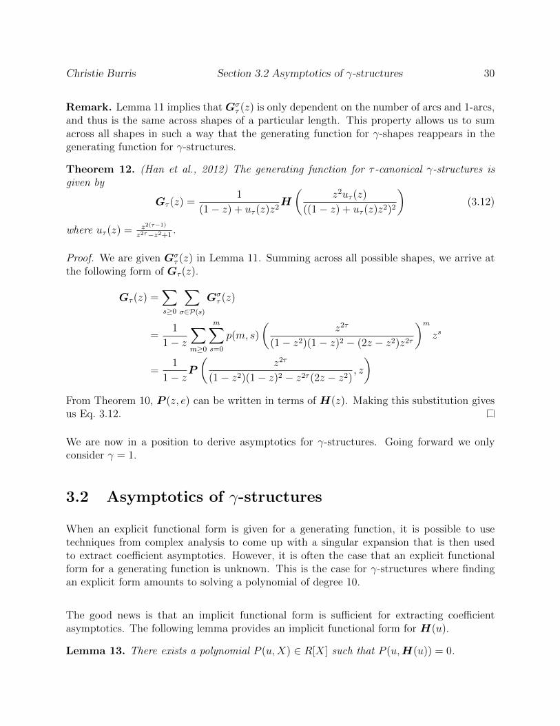
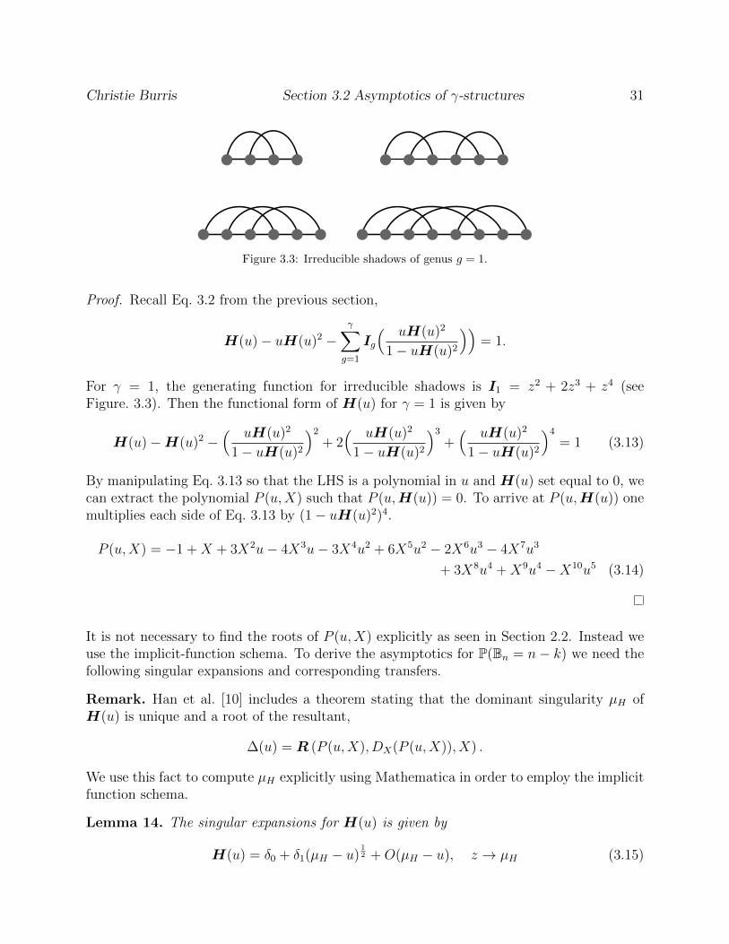
Figure 3.3: Irreducible shadows of genus g = 1.
Proof. Recall Eq. 3.2 from the previous section,
H(u)− uH(u)2 −γ∑g=1
Ig
( uH(u)2
1− uH(u)2
))= 1.
For γ = 1, the generating function for irreducible shadows is I1 = z2 + 2z3 + z4 (seeFigure. 3.3). Then the functional form of H(u) for γ = 1 is given by
H(u)−H(u)2 −( uH(u)2
1− uH(u)2
)2
+ 2( uH(u)2
1− uH(u)2
)3
+( uH(u)2
1− uH(u)2
)4
= 1 (3.13)
By manipulating Eq. 3.13 so that the LHS is a polynomial in u and H(u) set equal to 0, wecan extract the polynomial P (u,X) such that P (u,H(u)) = 0. To arrive at P (u,H(u)) onemultiplies each side of Eq. 3.13 by (1− uH(u)2)4.
P (u,X) = −1 +X + 3X2u− 4X3u− 3X4u2 + 6X5u2 − 2X6u3 − 4X7u3
+ 3X8u4 +X9u4 −X10u5 (3.14)
It is not necessary to find the roots of P (u,X) explicitly as seen in Section 2.2. Instead weuse the implicit-function schema. To derive the asymptotics for P(Bn = n− k) we need thefollowing singular expansions and corresponding transfers.
Remark. Han et al. [10] includes a theorem stating that the dominant singularity µH ofH(u) is unique and a root of the resultant,
∆(u) = R (P (u,X), DX(P (u,X)), X) .
We use this fact to compute µH explicitly using Mathematica in order to employ the implicitfunction schema.
Lemma 14. The singular expansions for H(u) is given by
H(u) = δ0 + δ1(µH − u)12 +O(µH − u), z → µH (3.15)
Christie Burris Section 3.2 Asymptotics of γ-structures 32
where δ0 = H(µH), δ1 = µ− 1
2H
√2µHPu(µH ,H(µH))PXX(µH ,H(µH))
. In addition, the asymptotics of the coeffi-
cients of H(u) are
[um]H(u) = cm−32µ−mH (1 +O(m−1)). (3.16)
where c = δ1µ12HΓ(−1
2)−1.
Proof. Consider the bivariate function P (u,X) given by Eq. 3.13. This function is a poly-nomial and consequently analytic at (µH ,H(µH)). By checking that the conditions of The-orem 4 hold for P (u,X), we are given the asymptotic expansion with the square root factor.The four conditions are
P (µH ,H(µ)) = 0, Pu(µH ,H(µH)) 6= 0, PX(µH ,H(µH)) = 0, PXX(µH ,H(µH)) 6= 0.
We check these conditions by explicitly computing the relevant partial derivatives and plug-ging in µH and H(µH) to each of them. Again the asymptotics follow from Theorem 2.
Lemma 15. The singular expansions for Gτ (z) is given by
Gτ (z) = θ0 + θ1(µ− z)12 + θ2(µ− z) +O((µ− z)
32 ), z → µ (3.17)
where θ0 = Gτ (µ). In addition, the asymptotics of the coefficients of Gτ (z) are
[zn]Gτ (z) = cn−32µ−n(1 +O(n−1)). (3.18)
where c = −θ1µ12 Γ(−1
2)−1.
Proof. Recall from Theorem 12 the expression for Gτ (z) in terms of H(u) given by Eq. 3.12,
Gτ (z) =1
(1− z) + uτ (z)z2H
(z2uτ (z)
((1− z) + uτ (z)z2)2
)where uτ (z) = z2(τ−1)
z2τ−z2+1.
Let the inner function composed with H(u) be labeled θ(z). First note that H(θ(z)) isanalytic at the origin with non-negative coefficients. By Pringsheim’s Theorem it must havea dominant singularity that lies on the positive real axis.
The candidates for its dominant singularities are the dominant singularities of θ(z) and thesolutions to θ(z) = µH . It is simple to check that a dominant singularity of θ(z) does not lieon the positive real line. Therefore, it must be the case that a solution to θ(z) = µH smallestin modulus must fall on the positive real line. By inspection, the positive real-valued solution
Christie Burris Section 3.3 The Longest Block 33
µ to θ(z) = µH smallest in modulus is unique. Thus H(θ(z)) falls under the supercriticalcomposition schema.
The singular expansion for H(θ(z)) is computed as the singular expansion of H(u) at z = µHwith the Taylor expansion of θ(z) at z = µ. Recall from Lemma 14 the singular expansionof H(u),
H(u) = δ0 + δ1(µH − u)12 +O(µH − u).
Then the composition with the Taylor series of θ(z) is
H(θ(z)) = δ0 + δ1(µH − (µH + θ′(µ)(z − µ) +O(z − µ)))12 +O(µ− z)
= δ0 + δ1θ′(µ)(µ− z)
12 +O(µ− z)
To arrive at the singular expansion of Gτ (z), we note that the singularities of the factor1
(1−z)+uτ (z)z2are a subset of the singularities of θ(z) which we have proven to be larger in
modulus than µ. Thus the dominant singularity of Gτ (z) is also µ and its singular expansionGτ (z) at z = µ is the product of the Taylor expansion of 1
(1−z)+uτ (z)z2and the singular
expansion of H(θ(z)). The result follows.
3.3 The Longest Block
The main result of this section is a precise statement regarding the expected length of thelongest irreducible component (block) of γ-structures for γ = 1 as the sequence length getsarbitrarily large. The method used to derive the expected length parallels the work of Liand Reidys in [15] for secondary structure. To this end, we define the random variable Bnrepresenting the length of the longest block in a structure of length n.
The average length of the longest rainbow is given by the expectation of the random vari-able Bn, labeled E[Bn]. The lemmas and theorems that follows provide the derivation of the
expectation E[Bn] and variance V[Bn], found to be on the order of n − O(n12 ) and O(n
32 )
respectively. In particular, we show that the expected length of the longest rainbow isn− αn 1
2 (1 + o(1)) with standard deviation√βn
34 (1 + o(1)).
The combinatorial class Gτ,n is the set of all τ -canonical γ-structures of length n now con-sidered as a sample space. We take the uniform probability function to form the finiteprobability space (Gτ,n,P) such that P(S) = 1
card(Gτ,n)for any S ∈ Gτ,n.
Christie Burris Section 3.3 The Longest Block 34
Consider the general definition of expectation given the discrete random variable Bn:
E[Bn] =∑ω∈Ω
Bn(ω)P(ω)
where ω is an event in the sample space Ω. We choose to partition the sample space intodisjoint events Bn = n− k for 1 ≤ k ≤ n. As such, E[Bn] can be rewritten
E[Bn] =n∑k=1
(n− k)P(Bn = n− k)
where P(Bn = n − k) is the probability that a γ-structure of length n has longest block oflength n− k since
⋃1≤k≤n(Bn = n− k) = Gτ,n. The following derivation of P(Bn = n− k) in
terms of generating function coefficients allows us to compute the expectation and variancethrough means of transfer theorems and singular expansions of the generating functions de-rived in the previous sections.
The probability that a given γ-structure of length n has longest block of length n− k is theratio of the number of structures with longest block length n − k to the total number ofstructures, assuming structures are uniformly sampled. In terms of coefficients of generatingfunctions, this ratio is the coefficient of some unknown generating function over [zn]Gτ (z).The generating function for γ-structures with longest block n−k proves to be too difficult tocompute directly as such a task requires a complex sequence of inclusion/exclusion argumentsthat do not lend themselves well to singularity analysis. As such, we note the following. IfG≤m(z) is the generating function for γ-structures whose blocks are of length less at mostto m, then the generating function for structures with longest block length exactly m is
G≤m(z)−G≤m−1(z).
Therefore,
P(Bn = n− k) =[zn](G≤n−k(z)−G≤n−k−1(z))
[zn]Gτ (z). (3.19)
It suffices to show how G≤m(z) can be expressed in terms of known generating functions.In the previous section we constructed the generating function Gτ (z) from inflating γ-matchings. Since we were able to derive a closed form for H(u), we were also granted aclosed form for Gτ (z) and thus computed the asymptotics of its coefficients. However, it isnow advantageous to consider γ-structures as sequences of blocks. Let T (z) be the generat-ing function for these irreducible components of γ-structures. Then the generating functionGτ (z) can be realized as
Gτ (z) =∑i≥0
(T (z))i =1
1− T (z).
Christie Burris Section 3.3 The Longest Block 35
Toward deriving an expression for P(Bn = n−k) in terms of coefficients of known generatingfunctions, let
T≤m(z) =m∑n=0
tnzn
be the truncated series representing the generating function for blocks of length at most m.Then the generating function for γ-structures with block length at most m is given by
G≤m(z) =∑i≥0
(T≤m(z))i =1
1− T≤m(z).
From here we are able to realize [zn](G≤n−k(z)−G≤n−k−1(z)) as the product of coefficientsof generating functions with known coefficient asymptotics. The following Lemma gives thisalternative form.
Lemma 16. For k ≤ n2− 1,
P(Bn = n− k) =[zk]Φ′(T (z))[zn−k]T (z)
[zn]Gτ (z)(3.20)
where Φ(z) = 11−z .
Proof. To arrive at Eq. 3.20, first recall Eq. 3.19,
P(Bn = n− k) =[zn](G≤n−k(z)−G≤n−k−1(z))
[zn]Gτ (z).
Consider the Taylor expansions of G≤n−k(z) and G≤n−k−1(z) as the compositions Φ(T≤n−k(z))and Φ(T≤n−k−1(z)) respectively, centered at T (z). We observe that both series terminate atthe second term.
G≤n−k(z) = Φ(T≤n−k(z)) =∑i≥0
Φ(i)(T (z))
i!(T≤n−k(z)− T (z))i,
G≤n−k−1(z) = Φ(T≤n−k−1(z)) =∑i≥0
Φ(i)(T (z))
i!(T≤n−k−1(z)− T (z))i (3.21)
For k ≤ n2− 1, the lowest power in the difference
T≤n−k(z)− T (z) = −∑j>n−k
tjzj.
is n2
+ 1. When it is raised to a power i ≥ 2 the degree of the series is necessarily ≥ n. Assuch, for i ≥ 2,
[zn](T≤n−k(z)− T (z))i = 0.
Christie Burris Section 3.3 The Longest Block 36
The same argument holds for [zn](T≤n−k(z)−T (z))i since the lowest power in the sum is n2.
As a result,
[zn]G≤n−k(z) = [zn](
Φ(T (z)) + Φ′(T (z))(T≤n−k(z)− T (z)))
[zn]G≤n−k−1(z) = [zn](
Φ(T (z)) + Φ′(T (z))(T≤n−k−1(z)− T (z)))
Plugging into Eq. 3.20 and simplifying the difference yields the desired form.
[zn](G≤n−k(z)−G≤n−k−1(z))
[zn]Gτ (z)=
[zn]Φ′(T (z))(T≤n−k(z)− T≤n−k−1(z))
[zn]Gτ (z)
=[zn]Φ′(T (z))tn−kz
n−k
[zn]Gτ (z)
The product zn−kΦ′(T (z)) shifts the coefficients of Φ′(T (z)) n− k positions to the left fromthe coefficient of zi to the coefficient of i+ n− k. Thus the coefficient of zn in Φ′(T (z))zn−k
is the coefficient of zk in Φ′(T (z)). Therefore,
[zn]Φ′(T (z))tn−kzn−k
[zn]Gτ (z)=
[zk]Φ′(T (z))[zn−k]T (z)
[zn]Gτ (z)
This completes the proof.
Remark. Although the 2 equations given by 3.21 are presented as Taylor series of a compo-sition, they can also be realized combinatorially as counting the same objects. By definition,G≤n−k(z) counts the number of γ-structures with block length at most n − k. To see that
the RHS counts these structures as well, consider Φ(i)(T (z))i!
as counting the way to mark the(i + 1) positions (unordered) where a block of length greater than n − k can be inserted.T≤n−k(z)−T (z) counts the possible structures that do not meet the maximum block lengthcriteria.
As such, the i-th term in the series counts the number of ways to insert i blocks of lengthgreater than n − k into a sequence of block followed by the alternating coefficient (−1)i.The term corresponding to i = 0 is exactly Gτ (z). Thus the full series is realized as theinclusion/exclusion principle applied to removing the set of structures containing at leastone block of length greater than n− k from the set of all possible structures.
Furthermore, The choice to restrict consideration of P(Bn = n − k) to cases k ≤ n2− 1
stems from the advantageous nature of the sums in 3.21; the choice of k affects the numberof nonzero coefficients in the sum. An expansion with nonzero terms from only T (z) andΦ′(T (z)) allows us to limit the amount of computation necessary later down the road. Giventhe coefficient asymptotics of T (z) and Φ′(T (z)), we are afforded an asymptotic approxima-tion of P(Bn = n− k).
Christie Burris Section 3.3 The Longest Block 37
Lemma 17. The singular expansions for T (z) and Φ′(T (z)) are the following
T (z) = 1− 1
θ0
+θ1
θ20
(µ− z)12 + θ3(µ− z) +O((µ− z)
32 ), (3.22)
Φ′(T (z)) = θ20 + 2θ0θ1(µ− z)
12 + θ4(µ− z) +O((µ− z)
32 ), (3.23)
as z → µ, where µ is the dominant singularity of Gτ (z), θ0 = Gτ (µ), and all other θis arepositive constants.
In addition, the asymptotics of the coefficients of T (z) and Φ′(T (z)) are given by
[zn]T (z) =c
θ20
n−32µ−n(1 +O(n−1))
[zn]Φ′(T (z)) = 2θ0cn− 3
2µ−n(1 +O(n−1)).
where c = −θ1µ12 Γ(−1
2)−1.
Proof. By construction,
T (z) =Gτ (z)− 1
Gτ (z).
One can view T (z) as the composition (φ Gτ )(z) where φ = 1− 1/z. Then the candidatesfor the dominant singularity of T (z) are the dominant singularity of Gτ (z) and the solutionto Gτ (z) = 0. Since Gτ (0) = 1 and Gτ (z) restricted to the positive real line is an increasingfunction, Gτ (z) > 0. Thus the dominant singularity of T (z) is the dominant singularityof Gτ (z), µ. Since φ(z) is analytic near Gτ (µ) This implies that the singular expansion ofT (z) is the Taylor expansion of φ(x) at θ0 composed with the singular expansion of Gτ (z).Namely,
1− 1
x= 1− 1
θ0
+x− θ0
θ20
+O((x− θ0)2),
1− 1
Gτ (z)= 1− 1
θ0
+1
θ20
(θ1(µ− z)12 + θ2(µ− z)) +O((µ− z)
32 )
= 1− 1
θ0
+θ1
θ20
(µ− z)12 + θ3(µ− z) +O((µ− z)
32 ).
It follows immediately from Theorem 2 that the transfer to coefficients is
[zn]T (z) =c
θ20
n−32µ−n(1 +O(n−1)).
Now consider Φ′(T (z)) = Gτ (z)2. Clearly the singularity of Φ′(T (z)) is µ since x2 is entire.The singular expansion of Gτ (z)2 is the singular expansion of Gτ (z) squared. The resultfollows.
Christie Burris Section 3.3 The Longest Block 38
We are now in a position to compute E[Bn]. The following manipulation results in a formthat allows us to make use of the coefficient asymptotics previously computed.
E[Bn] =n∑i=1
(n− k)P(Bn = n− k)
=n∑k=1
nP(Bn = n− k)−n∑k=1
kP(Bn = n− k)
= n−n2−1∑
k=1
kP(Bn = n− k)−n∑
k=n2
kP(Bn = n− k) (3.24)
The final lines of this manipulation take enough trickery they are afforded the lemmas thatfollow. Theorem 20 states the asymptotics of E[Bn] as well as V[Bn].
Lemma 18. For n→∞,
n2−1∑
k=1
kP(Bn = n− k) = αn12 (1 + o(1)) (3.25)
where α = 4cθ0
.
Proof. Since k ≤ n2− 1, Lemma 16 applies to P(Bn = n− k) in Eq. 3.25. Furthermore, the
coefficient asymptotics from Lemmas 15 and 17 bring us the desired approximation.
P(Bn = n− k) =[zk]Φ′(T (z))[zn−k]T (z)
[zn]Gτ (z)
=(2θ0ck
− 32µ−k)(c(n− k)−
32µ−(n−k))(1 +O(k−1))(1 +O((n− k)−1))
θ20cn
− 32µ−n(1 +O(n−1))
=2c
θ0
(1− k
n
)− 32k−
32 (1 +O(k−1))(1 +O(n−1)), n, k →∞.
The third equality holds because
(1 +O((n− k)−1))
(1 +O(n−1))=
(1 +O(n−1))
(1 +O(n−1))= (1 +O(n−1)).
In order for the asymptotics of [zk]Φ′(T (z)) to hold, k must approach infinity. For 1 ≤ k ≤n2− 1, this is not guaranteed. However, it is when k is bounded below by n as well. To
reconcile this, consider the sum in two pieces.∑1≤k≤n
2−1
kP(Bn = n− k) =∑
1≤k<n18
kP(Bn = n− k) +∑
n18≤k≤n
2−1
kP(Bn = n− k).
Christie Burris Section 3.3 The Longest Block 39
For 1 ≤ k < n18 , an approximation of the sum is derived without employing the coefficient
approximations. Since the probability function is bounded by 1,
∑k
kP(Bn = n− k) ≤∑k
k =n
18 (n
18 + 1)
2= o(n
12 ).
Note that the sum could have been separated at any place such that the final inequalityresulted in a term of order strictly less than 1/2.
Now consider n18 ≤ k ≤ n
2− 1. Since k is bounded above and below by powers of n, we can
take both k and n toward infinity and substitute the asymptotics of P(Bn = n− k) into thesecond sum. For n, k →∞,
∑k
kP(Bn = n− k) =2c
θ0
∑k
k(
1− k
n
)− 32k−
32 (1 +O(k−1))(1 +O(n−1))
=2c
θ0
n12
∑k
1
n
(1− k
n
)− 32(kn
)− 12(1 +O(k−1))(1 +O(n−1)). (3.26)
The sum in final line of the equality can be realized as a Riemann sum which converges toa Riemann integral. Recall the formula,∫ b
a
f(x) dx = limn→∞
1
n
n∑k=1
f(a+b− an
k).
For a = 0, b = 12, f(x) = (1−x)−
32x−
12 , the terms of the sum in the expression of P(Bn = n−k)
match that of the corresponding Riemann sum. The difference of the Riemann sum and thesum in line 3.26 is
n18∑
k=1
1
n
(1− k
n
)− 32(kn
)− 12
+4
n≤
n18∑
k=1
(1− n−78 )−
32n−
12 +
4
n
= n18 (1− n−
78 )−
32n−
12 +
4
n= o(1)
It follows that∑n
18≤k≤n
2−1
1
n
(1− k
n
)− 32(kn
)− 12
=
∫ 12
0
(1− x)−32x−
12 dx(1 + o(1)) = 2(1 + o(1))
Christie Burris Section 3.3 The Longest Block 40
We can eliminate dependence on k in the sum in line 3.26 by bounding (1 +O(k−1)) aboveand below by (1 + o(1)). Substituting the above asymptotics into the original sum,∑
k
P(Bn = n− k) =2c
θ0
n12
∑k
1
n
(1− k
n
)− 32(kn
)− 12(1 +O(k−1))(1 +O(n−1))
=4c
θ0
n12 (1 + o(1))(1 +O(n−1))
=4c
θ0
n12 (1 + o(1))
Setting α =4c
θ0
yields the desired result.
Lemma 19.∑
n2−1<k≤n
kP(Bn = n− k) = o(n12 ) as n→∞.
Proof. To invoke Lemma 16 once again, we make use of basic properties of probabilityfunctions. Namely, ∑
n2−1<k≤n
P(Bn = n− k) = 1−∑
1≤k≤n2−1
P(Bn = n− k).
Again the sum is broken up to yield advantageous asymptotics.∑n2−1<k≤n
kP(Bn = n− k)
≤ n(1−
∑1≤k≤n
2−1
P(Bn = n− k))
= n(1−
∑1≤k<n
25
P(Bn = n− k)−∑
n25≤k≤n
2−1
P(Bn = n− k)).
For 1 ≤ k < n25 , the coefficient asymptotics of T (z) and Gτ (z) can be substituted into
P(Bn = n− k). The resulting form is
P(Bn = n− k) =[xk]Φ′(T (z))[xn−k]T (z)
[zn]Gτ (z)
=[xk]Φ′(T (z))µk
θ20
(1− k
n
)− 32
(1 +O(n−1))
=[xk]Φ′(T (z))µk
θ20
(1 +O(n−35 ))(1 +O(n−1))
=[xk]Φ′(T (z))µk
θ20
(1 + o(n−12 )) (3.27)
Christie Burris Section 3.3 The Longest Block 41
The third inequality follows from applying the upper bound on k,(1− k
n
)− 32
< (1− n−35 )−
32 = (1 +O(n−
35 )).
The choice of approximation (1+o(n−12 )) becomes useful when the asymptotics are combined
in the final line of the proof.
To simplify notation, let bk = [zk]Φ′(T (z)).
∑1≤k<n
25
P(Bn = n− k) =∑
1≤k<n25
bkµk
θ20
(1 + o(n−12 ))
=( 1
θ20
∑k≥1
bkµk − 1
θ20
∑k≥n
25
bkµk)
(1 + o(n−12 ))
=(
1− 1
θ20
∑k≥n
25
bkµk)
(1 + o(n−12 ))
Recall that θ20 = Φ′(T (µ)). The first sum in the final equality is the generating function
Φ′(T (z)). Evaluating Φ′(T (z)) at µ yields Φ′(T (µ)) = (θ20)−1. Thus
1
θ20
∑k≥1
bkµk = 1.
Since k is now bounded below by a power of n in the final form of the original sum, we arein a position to apply the asymptotics of [zk]Φ′(T (z)).
(1− 1
θ20
∑k≥n
25
bkµk)
(1 + o(n−12 ))
=(
1− 2c
θ0
∑k≥n
25
k−32 (1 +O(k−1))
)(1 + o(n−
12 ))
=(
1− α
2
∑k≥n
25
k−32 +O
( ∑k≥n
25
k−52
))(1 + o(n−
12 ))
In order to eliminate dependence on k, we apply the well known asymptotics of the Hurwitz-Zeta function defined as
ζ(s, n) =∑i≥0
(n+ i)−s,
Christie Burris Section 3.3 The Longest Block 42
with the expansion ζ(s, n) = n1−s
s−1(1 +O(n−1)).∑
k≥n25
k−32 =
∑k≥0
(k + n25 )−
32 = 2n−
15 (1 +O(n−
25 )),
∑k≥n
25
k−52 =
∑k≥0
(k + n25 )−
52 =
2
3n−
35 (1 +O(n−
25 )).
Substituting the asymptotics into the final expression,∑1≤k<n
25
P(Bn = n− k)
=(
1− α
2
∑k≥n
25
k−32 +O
( ∑k≥n
25
k−52
))(1 + o(n−
12 ))
=(
1− αn−15 (1 +O(n−
25 )) +O(n−
35 ))
(1 + o(n−12 ))
= 1− αn−15 + o(n−
12 ).
Now consider n25 ≤ k ≤ n
2− 1. Since k is bounded below by n, we can let k, n → ∞ and
substitute the coefficient asymptotics of P(Bn = n− k),
∑n
25≤k≤n
2−1
P(Bn = n− k)
=2c
θ0
∑n
25≤k≤n
2−1
(1− k
n
)− 32k−
32 (1 +O(k−1))(1 +O(n−1)).
Recall in Lemma 18 that a sum similar to the one above was realized as an Riemann integral.However, the sum above is lacking an additional term k. Without this term the associatedintegral does not converge. As such, we instead approximate the sum using the Euler-Maclaurin summation formula given below.
∑a≤k<b
f(k) =
∫ b
a
f(x) dx+B1f(x)∣∣∣ba
+B2
2f ′(x)
∣∣∣ba
+R2,
where Bi’s are the Bernoulli numbers and R2 is on the order O( ∫ b
a|f ′′(x)| dx
). For more
detail on the derivation of this formula, see Ch. 9 in [9].
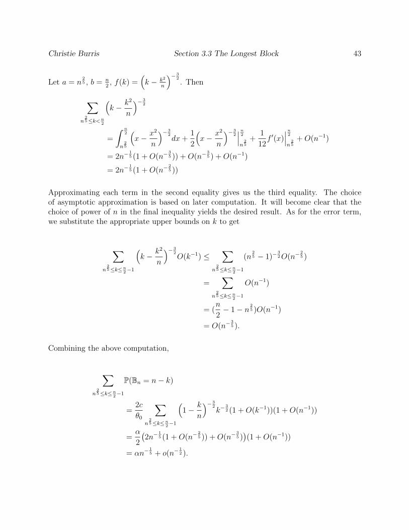
Christie Burris Section 3.3 The Longest Block 43
Let a = n25 , b = n
2, f(k) =
(k − k2
n
)− 32. Then
∑n
25≤k<n
2
(k − k2
n
)− 32
=
∫ n2
n25
(x− x2
n
)− 32dx+
1
2
(x− x2
n
)− 32∣∣∣n2n
25
+1
12f ′(x)
∣∣∣n2n
25
+O(n−1)
= 2n−15 (1 +O(n−
35 )) +O(n−
35 ) +O(n−1)
= 2n−15 (1 +O(n−
25 ))
Approximating each term in the second equality gives us the third equality. The choiceof asymptotic approximation is based on later computation. It will become clear that thechoice of power of n in the final inequality yields the desired result. As for the error term,we substitute the appropriate upper bounds on k to get
∑n
25≤k≤n
2−1
(k − k2
n
)− 32O(k−1) ≤
∑n
25≤k≤n
2−1
(n25 − 1)−
32O(n−
25 )
=∑
n25≤k≤n
2−1
O(n−1)
= (n
2− 1− n
25 )O(n−1)
= O(n−35 ).
Combining the above computation,
∑n
25≤k≤n
2−1
P(Bn = n− k)
=2c
θ0
∑n
25≤k≤n
2−1
(1− k
n
)− 32k−
32 (1 +O(k−1))(1 +O(n−1))
=α
2
(2n−
15 (1 +O(n−
25 )) +O(n−
35 ))(1 +O(n−1))
= αn−15 + o(n−
12 ).
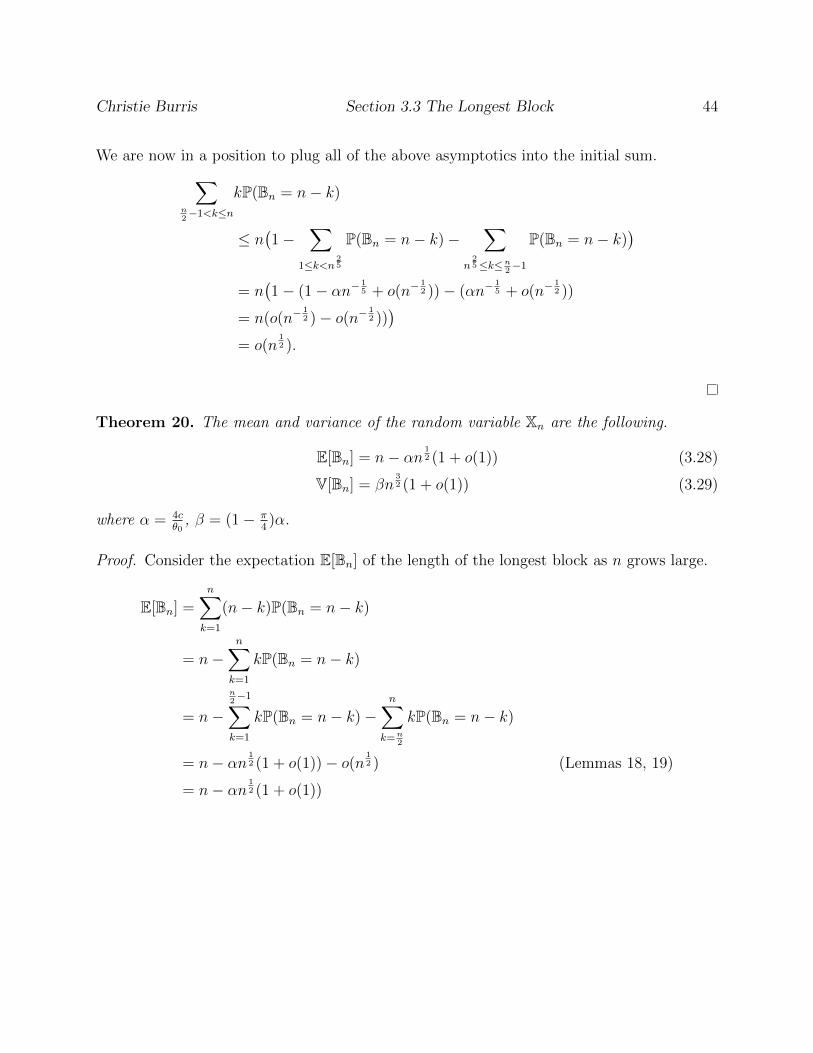
Christie Burris Section 3.3 The Longest Block 44
We are now in a position to plug all of the above asymptotics into the initial sum.∑n2−1<k≤n
kP(Bn = n− k)
≤ n(1−
∑1≤k<n
25
P(Bn = n− k)−∑
n25≤k≤n
2−1
P(Bn = n− k))
= n(1− (1− αn−
15 + o(n−
12 ))− (αn−
15 + o(n−
12 ))
= n(o(n−12 )− o(n−
12 )))
= o(n12 ).
Theorem 20. The mean and variance of the random variable Xn are the following.
E[Bn] = n− αn12 (1 + o(1)) (3.28)
V[Bn] = βn32 (1 + o(1)) (3.29)
where α = 4cθ0
, β = (1− π4)α.
Proof. Consider the expectation E[Bn] of the length of the longest block as n grows large.
E[Bn] =n∑k=1
(n− k)P(Bn = n− k)
= n−n∑k=1
kP(Bn = n− k)
= n−n2−1∑
k=1
kP(Bn = n− k)−n∑
k=n2
kP(Bn = n− k)
= n− αn12 (1 + o(1))− o(n
12 ) (Lemmas 18, 19)
= n− αn12 (1 + o(1))
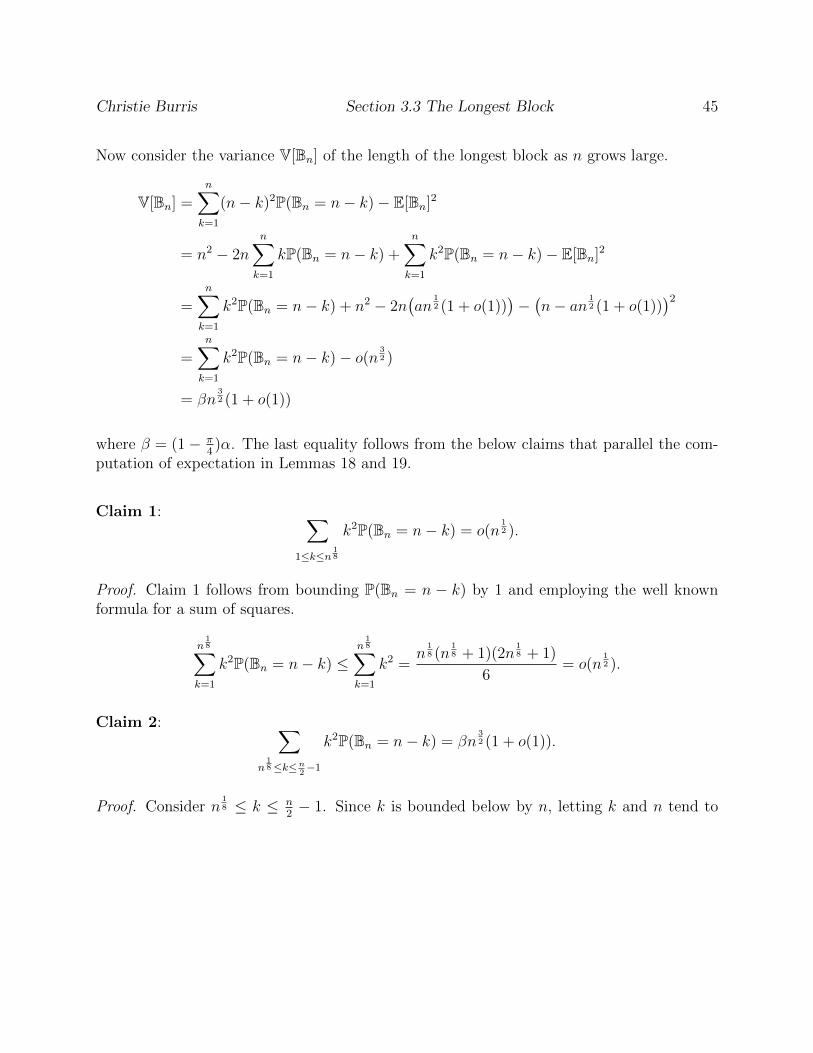
Christie Burris Section 3.3 The Longest Block 45
Now consider the variance V[Bn] of the length of the longest block as n grows large.
V[Bn] =n∑k=1
(n− k)2P(Bn = n− k)− E[Bn]2
= n2 − 2nn∑k=1
kP(Bn = n− k) +n∑k=1
k2P(Bn = n− k)− E[Bn]2
=n∑k=1
k2P(Bn = n− k) + n2 − 2n(an
12 (1 + o(1))
)−(n− an
12 (1 + o(1))
)2
=n∑k=1
k2P(Bn = n− k)− o(n32 )
= βn32 (1 + o(1))
where β = (1− π4)α. The last equality follows from the below claims that parallel the com-
putation of expectation in Lemmas 18 and 19.
Claim 1: ∑1≤k≤n
18
k2P(Bn = n− k) = o(n12 ).
Proof. Claim 1 follows from bounding P(Bn = n − k) by 1 and employing the well knownformula for a sum of squares.
n18∑
k=1
k2P(Bn = n− k) ≤n
18∑
k=1
k2 =n
18 (n
18 + 1)(2n
18 + 1)
6= o(n
12 ).
Claim 2: ∑n
18≤k≤n
2−1
k2P(Bn = n− k) = βn32 (1 + o(1)).
Proof. Consider n18 ≤ k ≤ n
2− 1. Since k is bounded below by n, letting k and n tend to
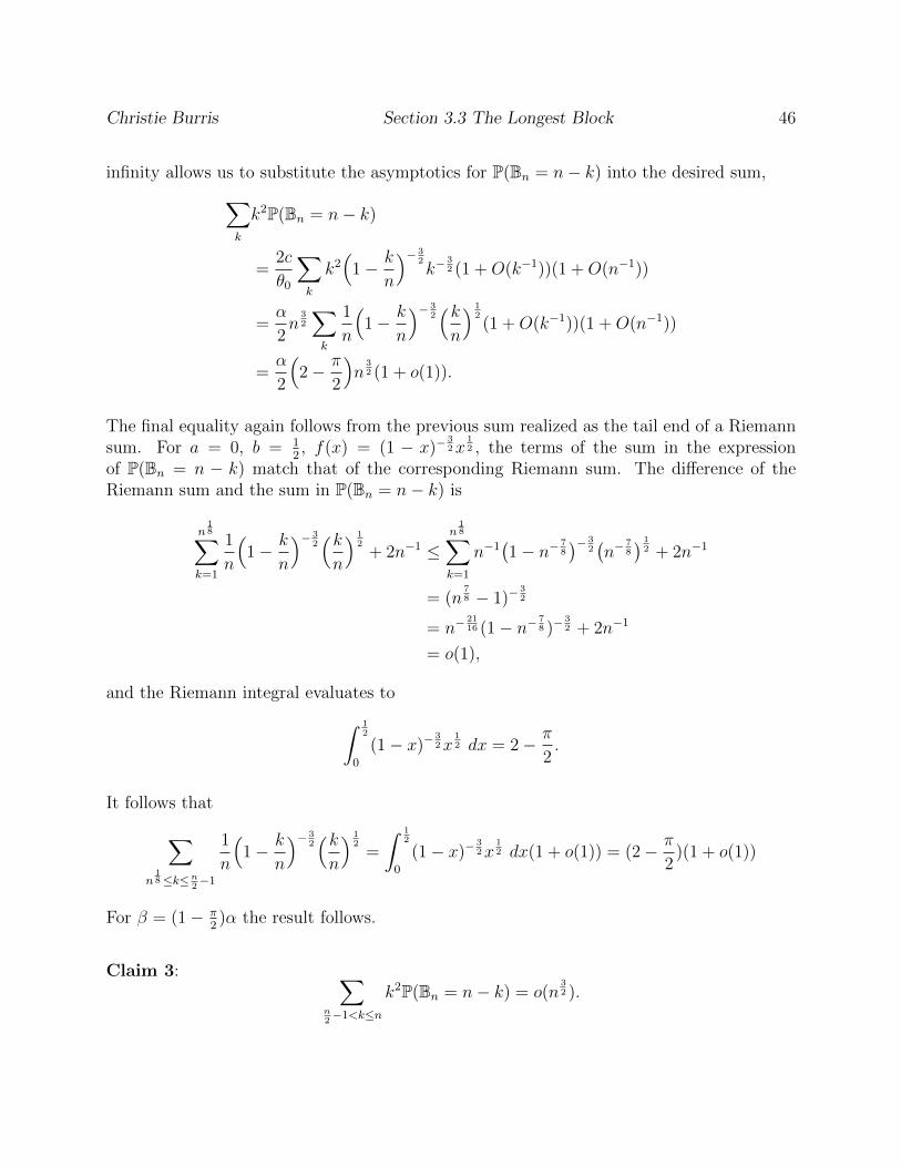
Christie Burris Section 3.3 The Longest Block 46
infinity allows us to substitute the asymptotics for P(Bn = n− k) into the desired sum,∑k
k2P(Bn = n− k)
=2c
θ0
∑k
k2(
1− k
n
)− 32k−
32 (1 +O(k−1))(1 +O(n−1))
=α
2n
32
∑k
1
n
(1− k
n
)− 32(kn
) 12(1 +O(k−1))(1 +O(n−1))
=α
2
(2− π
2
)n
32 (1 + o(1)).
The final equality again follows from the previous sum realized as the tail end of a Riemannsum. For a = 0, b = 1
2, f(x) = (1 − x)−
32x
12 , the terms of the sum in the expression
of P(Bn = n − k) match that of the corresponding Riemann sum. The difference of theRiemann sum and the sum in P(Bn = n− k) is
n18∑
k=1
1
n
(1− k
n
)− 32(kn
) 12
+ 2n−1 ≤n
18∑
k=1
n−1(1− n−
78
)− 32(n−
78
) 12 + 2n−1
= (n78 − 1)−
32
= n−2116 (1− n−
78 )−
32 + 2n−1
= o(1),
and the Riemann integral evaluates to∫ 12
0
(1− x)−32x
12 dx = 2− π
2.
It follows that∑n
18≤k≤n
2−1
1
n
(1− k
n
)− 32(kn
) 12
=
∫ 12
0
(1− x)−32x
12 dx(1 + o(1)) = (2− π
2)(1 + o(1))
For β = (1− π2)α the result follows.
Claim 3: ∑n2−1<k≤n
k2P(Bn = n− k) = o(n32 ).
Christie Burris Section 3.3 The Longest Block 47
Proof.∑n2−1<k≤n
k2P(Bn = n− k) ≤ n2∑
n2−1<k≤n
P(Bn = n− k)
= n2(
1−∑
1<k≤n25
P(Bn = n− k) +∑
n25<k≤n
2−1
P(Bn = n− k))
= n2(1− (1− an−15 + o(n−
12 ))− (an−
15 + o(n−
12 )))
= n2o(n−12 )
= o(n32 )
The second equality is computed in the proof of Lemma 19.
Remark. This powerful result implies that the distribution of Bn becomes increasingly moreconcentrated as n becomes large. Namely, E[Bn] is on the order larger than the standard
deviation,√V[Bn] = O(n
34 ). Because E[Bn] = n − O(n
12 ) > n
2, we can conclude that there
exists a unique longest block. To finalize the discussion on the longest block, Theorem 21gives the distribution of the difference in the length of the sequence and the length of thelongest block.
Theorem 21. For any t > 34,
limn→∞
P(n− Bn ≥ Ω(nt)) = 0 (3.30)
and for any k = o(n)
limn→∞
P(n− Bn = k) =[zk]Φ′(T (z))µk
θ20
. (3.31)
Proof. We apply Chebyshev’s Inequality to E[Bn] and V[Bn] given by Theorem 20 to arriveat Eq. 3.30. By Chebyshev’s Inequality,
P(|Bn − E[Bn]| ≥ m) ≤ V[Bn]
m2.
Set m = Ω(nt) for some t > 34. Taking the limit of both sides of the inequality allows us to
substitute the asymptotics provided in Theorem 20.
limn→∞
P(|Bn − E[Bn]| ≥ m) ≤ limn→∞
V[Bn]
m2
limn→∞
P(n− an12 − Bn ≥ Ω(nt)) ≤ lim
n→∞
O(n32 )
Ω(nt)2
limn→∞
P(n− Bn ≥ Ω(nt) + an12 ) = 0
limn→∞
P(n− Bn ≥ Ω(nt)) = 0
Christie Burris Section 3.3 The Longest Block 48
The third line follows from Ω(nt)2 > Ω(n32 ). Since probability functions are strictly positive,
the inequality becomes an equality.
Now consider k = o(n). Eq. 3.20,
P(Bn = n− k) =[zk]Φ′(T (z))[zn−k]T (z)
[zn]Gτ (z)
can be applied here since k ≤ n2− 1. Eq. 3.31 follows immediately from plugging in the
coefficient asymptotics of T (z) and Gτ (z).
Remark. Theorem 21 implies that the distribution of n− Bn a.a.s. converges to a discretelimit law. Eq. 3.30 says that, as n gets large, the probability that the difference betweenthe 5’-3’ distance of a γ-structure and the length of its longest block is on the order greaterthan n
34 is 0.
It is worth noting the special case k = n12 . Eq. 3.31 gives the limiting probability as
limn→∞
P(n− Bn = k) =[zk]Φ′(T (z))µk
θ20
.
Since in this case k →∞, we can apply the coefficient asymptotics of Φ′(T (z)) to the RHSof the equation.
limn→∞
P(n− Bn = n12 ) =
2n−34
θ0
As n gets large, P(n−Bn = n12 ) approaches 0. Contrast this with the expectation of n−Bn,
E[n− Bn] = n− E[Bn] = αn12 .
At first glance it appears contradictory that the probability that the difference in length ofstructure and length of longest block achieves the expected value be 0. Refer back to thedefinition of expectation,
E[Bn] =∑k≥0
(n− k)P(Bn = n− k).
Although P(Bn = n − k) approaches 0 when k is O(n12 ), the contribution from (n − k)
dominates and inevitably skews the expectation toward infinity. One naturally asks, whereon the length spectrum is the highest probability observed? It turns out that with highprobability, the tail end of the spectrum is observed. Corollary 21.1 provides information onblocks other than the longest one (these blocks are referred to as short).
Corollary 21.1. For all ε > 0 there exists an integer t(ε) such that
limn→∞
P(Bn ≥ n− t(ε)) ≥ 1− ε.
Christie Burris Section 3.4 The Spectrum of Blocks 49
Proof. Singularity analysis shows that φ′(T (z)) converges at µ. Following from an alternativedefinition of convergence, for every ε > 0 there exists an integer t(ε) such that for k > t(ε),∑
k>t(ε)
bkµk < ε,
where bk = [zk]φ′(T (z)). Additionally, for d = φ′(T (µ))−1∑k>t(ε)
dbkµk < ε.
By Theorem 21 the below list of algebraic manipulations hold.
limn→∞
P(Bn ≥ n− t(ε)) = limn→∞
∑k≤t(ε)
P(Bn = n− k)
=∑k≤t(ε)
dbkµk
=∑k≥1
dbkµk −
∑k>t(ε)
dbkµk
= dφ′(T (µ))− ε= 1− ε.
The discussion on short rainbows is continued to the next section.
3.4 The Spectrum of Blocks
As previously discussed, the field of analytic combinatorics also provides a framework tostudy properties of parameters of graphs such as: How many substructures of a particularkind appear in a random graph? In our case, we ask how many blocks of chosen length k ap-pear in uniformly sampled γ-structures of length n. The appearance of a second parameter,the number of blocks of a given length, shifts the nature of the problem slightly. Instead ofan ordinary generating function carrying information on one parameter (length), we employa bivariate generating function, Gτ,k(z, u) carrying information on two parameters. Themain result of this section is a statement regarding the limiting distribution of small blocksin γ-structures.
For fixed k, define the bivariate generating function
Gτ,k(z, u) =∑n,b
gτ,k(n, b)znub
Christie Burris Section 3.4 The Spectrum of Blocks 50
where gτ,k(n, b) is the count of γ-structure of length n containing b blocks of length k.
Define the random variable, Wk, to be the function from a given γ-structure to the count ofits blocks of length k. Namely, the set Wk,n = b is the set of γ-structures of length n with bblocks of length k.
The asymptotic behavior of Wk,n is, as before, intrinsically linked to the behavior of Gτ,k(z, u)near its singularities. The study of this behavior parallels nicely the OGF case due totheorems relating to uniform convergence and continuity expounded upon in Section 2. Assuch, we provide asymptotics of the probability generating function of Wk,n in order todetermine its limiting distribution.
Lemma 22. The bivariate generating function for the number of τ -canonical γ-structureswith minimum arc-length λ filtered by rainbows of length k is given by
Gτ,k(z, u) =1
1− r(z, u)(3.32)
where r(z, u) = T (z) + (u− 1)tkzk.
Proof. As before, γ-structures can be constructed by concatenating irreducible block com-ponents, represented by the power series
Gτ (z) =1
1− T (z)=∑i≥0
(T (z))i.
The coefficient corresponding to the n-th power of Gτ (z) is computed
[zn]Gτ (z) =∑
i1+...+im=n
ti1 · · · tim .
The coefficient corresponding to the n-th power of∑
i≥0(r(z, u))i differs by [zn]Gτ (z) suchthat when tk appears in the product, it is accompanied by u. The power of u in the productof coefficients corresponds to the number of appearances of a block of length k, as desired.Thus
Gτ,k(z, u) =∑i≥0
(r(z, u))i.
It suffices to show that (1−r(z, u)) has an inverse in Q[[z]] since, by construction, Gτ,k(z, u)(1−r(z, u)) = 1. A power series has an inverse in Q[[z]] if and only if its constant term is nonzero.Then 1 − r(z, u) has an inverse if the constant term of T (z) is different from 1. Since weassume there is no empty block, this is the case.
Christie Burris Section 3.4 The Spectrum of Blocks 51
For fixed n and k, the probability of the appearance of a γ-structure of length n with brainbows of length k is the ratio of the number of such structures to the total number ofstructures.
P(Wk,n = b) =gτ,k(n, b)
gτ (n)=
[znub]Gτ,k(z, u)
[zn]Gτ (z).
The probability generating function for Wk,n is∑b≥0
P(Wk,n = b)ub =[znub]Gτ,k(z, u)
[zn]Gτ (z)ub.
The coefficient asymptotics of Gτ (z) are given by
[zn]Gτ,k(z, u) = cn−32µ−n(1 + o(1)), n→∞,
where c = θ1µ12 Γ(−1
2)−1.
To derive the asymptotics of [znub]Gτ,k(z, u), we consider Gτ,k(z, u) as a function of z param-eterized by u in order to employ the perturbation analysis given by Flajolet and Sedgewick(refer to Section 2.2). It suffices to prove that Gτ,k(z, u) has a uniform asymptotic expansionwith respect to u and to specify how the coefficient, power, and singularity of the asymptoticsof Gτ (z) change by perturbing u.
Lemma 23. r(z, u) has a uniform asymptotic expansion with respect to u ∈ 1± o(1).
Proof. It suffices to show that (u− 1)tkzk has a uniform asymptotic expansion as T (z) does
not depend on u.
The Taylor expansion of (u− 1)tkzk at z = µ is
(u− 1)tkzk = (u− 1)tk
(µk + kµk−1(µ− z) + . . .+O((µ− z)m)
). (3.33)
For given m < k, Eq. 3.33 is a uniform expansion if there exists L (independent of u) and afixed neighborhood N(µ) such that for all u ∈ Nε(1), z ∈ N(µ),
|(u− 1)tkk(k − 1) · · · (k −m)µk−m(µ− z)m| ≤ L|(µ− z)m|.
Let L = εtkk(k − 1) · · · (k − m)µk−m where ε is the radius of the neighborhood around 1bounding u. The result follows.
Theorem 24. The dominant singularity of Gτ,k(z, u) is the dominant singularity µ of Gτ (z).The singular expansion for Gτ,k(z, u) is given by
Gτ,k(z, u) = Φ(r(µ, u)) + Φ′(r(µ, u))θ1
θ20
(µ− z)12 (1 + o(1)) (3.34)
Christie Burris Section 3.4 The Spectrum of Blocks 52
and the asymptotics of the coefficients of Gτ,k(z, u) are given by
[zn]Gτ,k(z, u) =Φ′(r(µ, u))
θ20
cn−32µ−n(1 + o(1)) (3.35)
where c = θ1µ12 Γ(−1
2)−1.
Proof. Consider Gτ,k(z, u) = Φ(r(z, u)) for fixed u such that u ∈ 1± o(1). The singularitiesof Gτ,k(z, u) are the singularities of r(z, u) and the solution to r(z, u) = 1.
µ, also the dominant singularity of T (z), is the dominant singularity of r(z, u) since (u −1)tkµ
k is constant and thus entire. If r(z, u) < 1 for u ∈ 1± o(1), then the dominant singu-larity of Gτ,k(z, u) is also µ. By inspection, r(z, u) < 1 for u ∈ 1± o(1), |z| ≤ µ.
Consequently, Gτ,k(z, u) falls under the subcritical paradigm. As such, the singular ex-pansion of Gτ,k(z, u) is computed as the composition of the Taylor expansion of Φ(z) atz = r(µ, u) and the singular expansion of r(z, u) at z = µ.
The singular expansion of r(z, u) at z = µ is the sum of the singular expansion of T (z) atz = µ and the Taylor expansion of (u− 1)tkz
k at z = µ.
r(z, u) = 1− 1
θ0
+θ1
θ20
(µ− z)12 (1 + o(1)) + (u− 1)tkµ
k +O(µ− z)
= 1− 1
θ0
+ (u− 1)tkµk +
θ1
θ20
(µ− z)12 (1 + o(1))
= r(µ, u) +θ1
θ20
(µ− z)12 (1 + o(1))
The Taylor expansion of Φ(z) at z = r(µ, u) is
Φ(z) = Φ(r(µ, u)) + Φ′(r(µ, u))(z − r(µ, u)) +O((z − r(µ, u))2)
Combining the two expansions gives us Eq. 3.34.
Φ(r(z, u)) = Φ(r(µ, u)) + Φ′(r(µ, u))(r(µ, u) +θ1
θ20
(µ− z)12 (1 + o(1))− r(µ, u))
= Φ(r(µ, u)) + Φ′(r(µ, u))θ1
θ20
(µ− z)12 (1 + o(1))
Eq. 3.35 follows immediately from Theorem 2.

Christie Burris Section 3.4 The Spectrum of Blocks 53
Theorem 24 provides the asymptotics used in the main result of this section.
Theorem 25. For fixed k, the limit law of Wk,n is a negative binomial distribution NB(2, t)where
t =tkµ
k
1− T (µ) + tkµk,
and tk = [zk]T (z). Consequently, the expectation and variance for Wk,n are given by
E[Wk,n] =2tkµ
k
1− T (µ), V[Wk,n] =
2t
(1− t)2.
Proof. To prove that for fixed k, the limit law of Wk,n is a negative binomial distributionNB(2, t) for t defined above, it suffices to show that the probability generating function ofthe limit distribution can be expressed as
pk(u) =
(1− t
1− tu
)2
.
Plugging in the asymptotics derived in Theorem 24 to the probability generating functionderived at the beginning of this section, we arrive at the desired form.
pk(u) = limn→∞
∑b
P(Wk,n = b)ub
= limn→∞
[znub]Gτ,k(z, u)
[zn]Gτ (z)ub
= limn→∞
[zn]Gτ,k(z, u)
[zn]Gτ (z)
= limn→∞
Φ′(r(µ,u))
θ20cn−
32µ−n(1 + o(1))
cn−32µ−n(1 + o(1))
=Φ′(r(µ, u))
θ20
=
(1− T (µ)
1− T (µ)− (u− 1)tkµk
)2
The final equality follows from noting θ20 = Φ′(T (µ)) and Φ′(z) = 1
(1−z)2 . Solving for t in theequation
1− T (µ)
1− T (µ)− (u− 1)tkµk=
1− t1− tu
yields the desired expression for t. The mean and variance are immediate form properties ofthe negative binomial distribution NB(2, t).
Christie Burris Section 3.4 The Spectrum of Blocks 54
This completes the analysis of the block length spectrum for γ-structures. We have providedthe expectation and variance for the unique longest block, and obtained the limiting distri-bution of the distribution of blocks of (finite) length k. We put these results in context withother subsets of RNA structures in the discussion.
Chapter 4
Discussion
In Section 3 we prove that the expected length of the longest block for γ-structures isE[Bn] = n−O(n
12 ) with standard deviation V[Bn]
12 = O(n
34 ) by treating the structures first
as combinatorial objects as then as objects in a probability space. As such, we are able toderive asymptotic appximations of generating function coefficients carrying information onthe number of γ-structures of a given length. These generating function coefficients arise inthe definitions of probability and expectation of the length of the longest block. Further-more, we show in Corollary 21.1 that with high probability, the second longest block hasfinite length. Namely, for choice of an integer t(ε), the probability that the length of thelongest block has length n − t(ε) is close to 1. Thus the second longest rainbow has lengthbounded by t(ε) with high probability.
Recall the initial question prompting this research: How does the length of the longest rain-bow change as the complexity of the structures increases? As mentioned previously, theanalysis on the expected block length of a γ-structure for γ = 1 parallels the analysis ofrainbow length for secondary structure in [15] and the results have deep similarities. Lemma
1 in [15] gives the expectation of the length of the longest rainbow as n− an 12 (1 + o(1)) and
with standard deviation√bn
34 (1 + o(1)) where a and b differ from α and β in Theorem 20
of this paper.
What leads on that these results should be so similar? It turns out that secondary structurescan be realized as γ-structures such that γ = 0. Recall that γ-structures are decomposedinto blocks with maximal irreducible shadow of genus at most γ. When γ > 0, these shadowsinclude crossing arcs. However, for γ = 0 this irreducible shadow is a single rainbow.
In this way secondary structures are decomposed into irreducible components that are iden-tified by a maximal rainbow. Furthermore, an irreducible structure of length m has longest
55

Christie Burris Chapter 4 Discussion 56
rainbow of length m − 1. Thus the expected length of the longest rainbow is the expectedlength of the longest irreducible component.
Table 4.1 gives the coefficients αγ in the expectation of the longest block n−αγn12 (1 + o(1))
for γ-structures for varying γ.
Table 4.1: Growth coefficients αγ for the expectation of the longest block in γ-structures, 0 ≤ γ ≤ 3
γ 0 1 2 3
αγ 2.804 1.416 0.964 0.734
Appendix A
Analyticity
The following list of definitions and theorems provides the background necessary to performsingularity analysis. As such, all information can be found throughout [6].
Definition 10. A region Ω is an open, connected subset of the complex plane.
Definition 11. A function f(z) defined over a region Ω is analytic at a point z0 ∈ Ω if, forz in some open disc centered at z0 and contained in Ω, it is representable by a convergentpower series expansion
f(z) =∑i≥0
fi(z − z0)i.
A function is analytic in a region Ω iff it is analytic at every point of Ω.
Similarly, a converging power series is analytic inside its radius of convergence. Where afunction ceases to be analytic, or where a power series fails to converge is an essential partof the analysis of Section 3.
Definition 12. The point z = a is called a singularity of the complex function f(z) if fis not analytic at a, but every neighborhood Nε(a) around a contains at least one point atwhich f(z) is analytic. A dominant singularity is a singularity of smallest modulus, or ratherclosest to the origin. Note that the dominant singularity need not be unique.
Theorem 26. A function f(z) analytic at the origin, whose expansion at the origin has afinite radius of convergence R, necessarily has a singularity on the boundary of its disc ofconvergence |z| = R.
Theorem 26 relates analyticity to the location of a function’s singularities in a powerful way.Namely, a converging power series must have at least one singularity on the boundary of itsdisc of convergence.
57
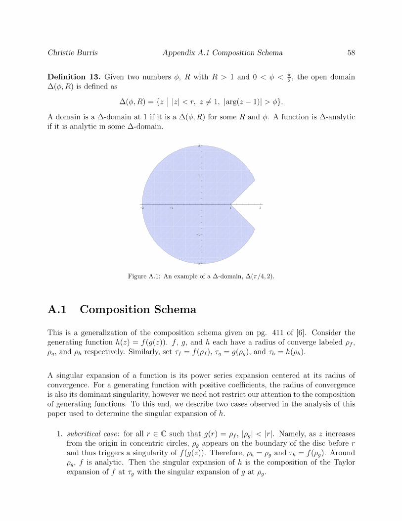
Christie Burris Appendix A.1 Composition Schema 58
Definition 13. Given two numbers φ, R with R > 1 and 0 < φ < π2, the open domain
∆(φ,R) is defined as
∆(φ,R) = z∣∣ |z| < r, z 6= 1, |arg(z − 1)| > φ.
A domain is a ∆-domain at 1 if it is a ∆(φ,R) for some R and φ. A function is ∆-analyticif it is analytic in some ∆-domain.
-2 -1 1 2
-2
-1
1
2
Figure A.1: An example of a ∆-domain, ∆(π/4, 2).
A.1 Composition Schema
This is a generalization of the composition schema given on pg. 411 of [6]. Consider thegenerating function h(z) = f(g(z)). f , g, and h each have a radius of converge labeled ρf ,ρg, and ρh respectively. Similarly, set τf = f(ρf ), τg = g(ρg), and τh = h(ρh).
A singular expansion of a function is its power series expansion centered at its radius ofconvergence. For a generating function with positive coefficients, the radius of convergenceis also its dominant singularity, however we need not restrict our attention to the compositionof generating functions. To this end, we describe two cases observed in the analysis of thispaper used to determine the singular expansion of h.
1. subcritical case: for all r ∈ C such that g(r) = ρf , |ρg| < |r|. Namely, as z increasesfrom the origin in concentric circles, ρg appears on the boundary of the disc before rand thus triggers a singularity of f(g(z)). Therefore, ρh = ρg and τh = f(ρg). Aroundρg, f is analytic. Then the singular expansion of h is the composition of the Taylorexpansion of f at τg with the singular expansion of g at ρg.
Christie Burris Appendix A.2 Analytic Transfer 59
2. supercritical case: there exists r ∈ C such that g(r) = ρf and |r| < |ρg|. Namely, as zincreases from the origin in concentric circles, r appears on the boundary of the discbefore ρg and thus triggers a singularity of f(g(z)). Therefore, ρh = r and τh = f(r).Around r, g is analytic, so the singular of h is the composition of the singular expansionof f at ρf with the Taylor expansion of g at r.
In the case where f and g have non-negative coefficients, the radii of convergence are thedominant singularities, which from Pringsheim’s Theorem are known to be positive and realvalued. Thus one can restrict the attention of r to the positive real line as h will also satisfythe conditions of Pringsheim’s Theorem.
A.2 Analytic Transfer
Theorem 27. (Flajolet, Sedgewick) Let α be an arbitrary complex number in C\Z≤0.The coefficient of zn in
f(z) = (1− z)−α
admits for large n a complete asymptotic expansion in descending powers of n,
[zn]f(z) ∼ nα−1
Γ(α)(1 +O(n−1)).
Proof. Here we provide a sketch of the proof. The full details can be found in [5].
Our interest is in approximating [zn]f(z) as n grows large. To do so, consider Cauchy’scoefficient formula
[zn]f(z) =1
2πi
∫Cf(z)
dz
zn+1,
a consequence of Cauchy’s Integral Formula where C is a contour that encircles the originsuch that f(z) is analytic in the disc bounded by C. For f(z) = (1−z)−α, any radius less than1 suffices. The contour can be deformed without changing the value of the integral so longas the region preserves analyticity. By specifying an advantageous contour and performinga change of variable, one can approximate the above integral by the Γ-function. In doing sowe arrive at the asymptotics.
The contour is most easily specified by a series of deformations. Begin with C0, a circle ofradius 1
2centered at z = 0. Deform C0 into C1, a circle with larger radius R > 1, and a notch
H(n) that wraps around the half line R≥1, defined piecewise as
H(n) = H−(n) ∪H+(n) ∪H(n)
Christie Burris Appendix A.2 Analytic Transfer 60
with H−(n) = z = ω − i
n, 1 ≤ ω ≤ R
H+(n) = z = ω + in, 1 ≤ ω ≤ R
H(n) = z = ω − eiϕ
n, ϕ ∈ [−π
2, π
2]
Note that as R tends to infinity,
(1− z)−α
zn+1= O(R−n).
Namely, (1 − z)−α grows in modulus as O(R) for α fixed. This can seen by representing(1− z)−α as (Reiθ)−α, however the details are omitted here.
Now consider the change of variable z = 1 + tn. The integrand is transformed into
1
2πi
∫C1+H(n)
(1− z)−αdz
zn+1=
1
2πi
∫C1+H
(−tn
)−α(1 +
t
n
)−n−11
ndt
=nα−1
2πi
∫H
(−t)−α(
1 +t
n
)−n−1
dt+O(R−n)
where
H =
H− = z = ω − i, ω ≥ 0H+ = z = ω + i, ω ≥ 0H = z = −eiϕ, ϕ ∈ [−π
2, π
2]
by letting R tend to infinity. The notch H is commonly referred to as a Hankel contourused to represent the Γ-function. H starts at positive infinity, winds around the origin at adistance 1 in the positive direction from the real axis, then approaches infinity again alongthe line z = −i.
Recall the asymptotic form of the exponential function
e−t = limn→∞
(1 +
t
n
)−n.
Then
limn→∞
(1 +
t
n
)−n−1
= e−t limn→∞
(1 +
t
n
)−1
= e−t(1 +O(n−1)).
Now the integrand can be rewritten,
nα−1
2πi
∫H
(−t)−α(
1 +t
n
)−n−1
dt =nα−1
2πi
∫H
(−t)−αe−tdt (1 +O(n−1)).
Christie Burris Appendix A.2 Analytic Transfer 61
Hankel’s Formula for the Γ-function relates the integral to Γ(s)−1,
Γ(s)−1 =−1
2πi
∫H
(−t)−se−tdt.
Lastly,
[zn](1− z)−α =nα−1
Γ(α)(1 +O(n−1)), n→∞.
Bibliography
[1] Anderson, J. E., Huang, F. W., Penner, R. C., Reidys, C. M. (2012) Topology of RNA-RNA InteractionStructures. Journal of Computational Biology. 19, 928-943.
[2] Chen, W. Y., Han, H. S., Reidys, C. M. (2009) Random k-noncrossing RNA structures. Proceedings ofthe National Academy of Sciences. 106(52) 22061-22066.
[3] Crick, F. H. C. (1958) On protein synthesis. Symp. Society of Experimental Biology. 12, 138–163.
[4] Ellis-Monaghan, J. and Moffatt, I. (2013) Graphs on Surfaces: Dualities, Polynomials, and Knots.Springer-Verlag New York.
[5] Flajolet, P. and Odlyzko, A (1990) Singularity Analysis of Generating Functions. Journal of DiscreteMathematics 3(2), 216-240.
[6] Flajolet, P. and Sedgewick, R. (2009). Analytic Combinatorics. Cambridge University Press.
[7] Fu, B. M., Han, H. S., Reidys, C. M. (2015) On RNA-RNA interaction structures of fixed topologicalgenus. Mathematical Biosciences. 262, 88-104.
[8] Gorodkin, J. and Ruzzo, W. L. (Eds.). (2014). RNA Sequence, Structure, and Function: Computationaland Bioinformatic Methods. New York, NY: Springer.
[9] Graham, R., Knuth, D., Patashnik, O. (1994) Concrete Mathematics: A Foundation for ComputerScience. Addison-Wesley.
[10] Han, H. S., Li, T. X., Reidys, C. M. (2014) Combinatorics of γ-structures. Journal of ComputationalBiology, (21), 591-608.
[11] Han, H. S., Reidys, C. (2012) The 5’-3’ Distance of RNA Secondary Structures. Journal of Computa-tional Biology. 19, 867-878.
[12] Huang, F. W., Nebel, M. E., Reidys, C. M. (2013) Shapes of topological RNA structures. MathematicalBiosciences 245, 216-225.
[13] Huang, F. W. D. and Reidys, C. M. (2012) On the combinatorics of sparsification. Algorithm. Mol.Biol. 7(28).
[14] Lander, E. S. (2011) Initial impact of the sequencing of the human genome. Nature. 470, 187–197.
[15] Li, T. X., Reidys, C. M. (2018). The rainbow-spectrum of RNA secondary structures. Bulletin ofMathematical Biology.
62
Christie Burris Appendix A.2 Analytic Transfer 63
[16] Mercer, T. R., Dinger, M. E., Mattick, J. S. (2009) Long non-coding RNAs: insights into function.Nature Reviews Genetics 10. 155-159.
[17] Mohl, M., Salari, R., Will, S., Backofen, R., Sahinalp, S. C. (2010) Sparsification of RNA structureprediction including pseudoknots. Alg. for Mol. Biology. 5(39).
[18] Nebel, M. E. and Weinberg, F. (2012) Algebraic and combinatorial properties of common RNA pseu-doknot classes with applications. J. Comput. Biol. 19, 1134-1150.
[19] Penner, R. C. and Waterman, M. S. (1993) Spaces of RNA secondary structures. Adv. Math. 101(31).
[20] Reidys, C. M. (2011) Combinatorial Computational Biology of RNA. Springer.
[21] Thomassen, C. (1989) The graph genus problem is NP-complete. J. Algorithms. 10(4) 568-576.
[22] Tinoco, I. and Bustamante, C. (1999) How RNA Folds. Journal of Molecular Biology. 293, 271–281.
[23] Von, M., Vernizzi, G., Zee, A., Orland, H. (2008) Topological Classification of RNA Structures. Journalof Molecular Biology. 379(4), 900-911.
[24] Watson, J. (1965). Molecular Biology of the Gene, Volume 1.
[25] Yoffe, A. M., Prinsen, P., Gelbart, W. M., Ben-Shaul, A. (2011) The ends of a large RNA molecule arenecessarily close. Nucleic Acids Research. 39(1) 292-299.