The Effects of Differential Rotation on the Spectral ...
74
i The Effects of Differential Rotation on the Spectral Energy Distribution and Line Profiles for Models of the Rapidly Rotating Star α Oph by Diego Casta ˜ neda A Thesis Submitted to Saint Mary’s University, Halifax, Nova Scotia in Partial Fulfillment of the Requirements for the Degree of Master of Science in Astronomy (Department of Astronomy and Physics) December 18, 2012, Halifax, Nova Scotia © Diego Casta ˜ neda, 2012 Approved: Dr. Robert Deupree Supervisor Approved: Dr. Ian Short Examiner Approved: Dr. Philip Bennett Examiner Date: December 18, 2012.
Transcript of The Effects of Differential Rotation on the Spectral ...
i
The Effects of Differential Rotation on the Spectral Energy
Distribution and Line Profiles for Models of the Rapidly Rotating
Star α Oph
by
Diego Castaneda
A Thesis Submitted to Saint Mary’s University, Halifax, Nova Scotia in Partial Fulfillmentof the Requirements for the Degree of Master of Science in Astronomy
(Department of Astronomy and Physics)
December 18, 2012, Halifax, Nova Scotia
© Diego Castaneda, 2012
Approved:Dr. Robert Deupree
Supervisor
Approved:Dr. Ian Short
Examiner
Approved:Dr. Philip Bennett
Examiner
Date: December 18, 2012.

ii
Acknowledgements
First, I would like to thank my supervisor, Dr. Robert Deupree for giving me the op-
portunity to work with him over the last two years; it has been a great experience. His
guidance, patience and wisdom propelled this work forward, and there still are some great
things to come. I would also like to thank Dr. Ian Short for all his help with PHOENIX and
modelling atmospheres, a key component our calculations. I would also like to thank Drs.
Ian Short and Phillip Bennet for being part of my defense committee.
I especially would like to thank Compute Canada (ACEnet), the Canada Foundation
for Innovation (CFI), the Nova Scotia Research Innovation Trust (NSRIT), and Saint Mary’s
University for providing all the computational tools necessary to complete this work.
Thanks to my family for all the help and cheering up from far away. I also appreciate
all the good times and discussions with my fellow graduate students, Liz, Jason, Patrick,
Michael, Mitch, Kirsten, Sherry and James. Finally, special thanks to Anneya, TPT and
Lambert for sitting with me for many hours while working on this document, providing
me with help, laughs and stories that kept me moving forward.
Contents
1 Introduction 1
Introduction 1
1.1 Background . . . . . . . . . . . . . . . . . . . . . . . . . . . . . . . . . . . . . 1
1.1.1 Modelling Rotating Stars . . . . . . . . . . . . . . . . . . . . . . . . . 4
1.2 α Oph . . . . . . . . . . . . . . . . . . . . . . . . . . . . . . . . . . . . . . . . . 10
2 Methods 15
2.1 The synthetic SED of a rotating star . . . . . . . . . . . . . . . . . . . . . . . 15
2.1.1 ROTORC . . . . . . . . . . . . . . . . . . . . . . . . . . . . . . . . . . . 17
2.1.2 PHOENIX . . . . . . . . . . . . . . . . . . . . . . . . . . . . . . . . . . 19
2.1.3 CLIC . . . . . . . . . . . . . . . . . . . . . . . . . . . . . . . . . . . . . 21
2.2 This work . . . . . . . . . . . . . . . . . . . . . . . . . . . . . . . . . . . . . . 23
3 Matching the SED of α Oph 26
3.1 Rotating Models . . . . . . . . . . . . . . . . . . . . . . . . . . . . . . . . . . . 29
3.2 Results . . . . . . . . . . . . . . . . . . . . . . . . . . . . . . . . . . . . . . . . 34
iii
CONTENTS iv
4 Lines 42
5 Conclusions 54
Bibliography 58
List of Figures
2.1 Illustration of various differential rotation laws for different values of β. The
value of a was chosen to be 2 and ω0 is 1 + aβ for this specific plot. . . . . . 18
2.2 CLIC calculated SED for 3 different inclinations of a specific rotating model
filtered with a boxcar filter of 50A. . . . . . . . . . . . . . . . . . . . . . . . . 23
3.1 Ultraviolet data from the IUE and OAO2 missions compared . . . . . . . . . 30
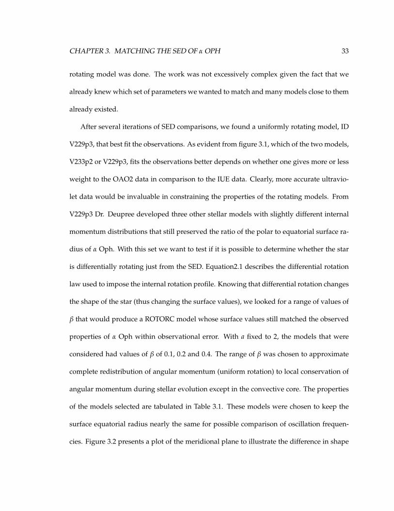
3.2 Cross section of the selected uniform rotating model (Blue curve) and the
highest differentially rotating model with β = 0.4 (Red curve). . . . . . . . . 34
3.3 Model suite vs. observation data . . . . . . . . . . . . . . . . . . . . . . . . . 37
3.4 UV and visible enlargements of the synthetic SEDs and the observations . . 38
3.5 Percentage of flux lost from the V229p3 model when the polar region is ex-
cluded from the calculation. We set the polar region to be between 0◦ − 30◦,
and 150◦ − 180◦ in latitude. . . . . . . . . . . . . . . . . . . . . . . . . . . . . 40
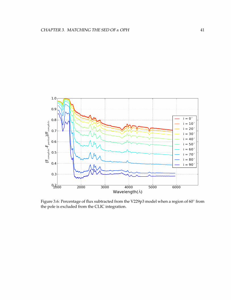
3.6 Percentage of flux subtracted from the V229p3 model when a region of 60◦
from the pole is excluded from the CLIC integration. . . . . . . . . . . . . . 41
v
LIST OF FIGURES vi
4.1 Line features surrounding 2360A . . . . . . . . . . . . . . . . . . . . . . . . . 44
4.2 Line features surrounding 2382A . . . . . . . . . . . . . . . . . . . . . . . . . 44
4.3 Line features surrounding 2406A . . . . . . . . . . . . . . . . . . . . . . . . . 45
4.4 Line at 2599A . . . . . . . . . . . . . . . . . . . . . . . . . . . . . . . . . . . . 45
4.5 Final UV selected line: Mg H/K . . . . . . . . . . . . . . . . . . . . . . . . . . 46
4.6 CaII line at 3934A . . . . . . . . . . . . . . . . . . . . . . . . . . . . . . . . . . 48
4.7 Line features in the range between 4212A− 4232A . . . . . . . . . . . . . . . 48
4.8 Line features surrounding 4620A . . . . . . . . . . . . . . . . . . . . . . . . . 49
4.9 Line features between 5203A− 5223A . . . . . . . . . . . . . . . . . . . . . . 49
4.10 Line features between 5223A− 5240A . . . . . . . . . . . . . . . . . . . . . . 50
4.11 Line profile comparison between the best-fit spherical atmospheric model in
NLTE and the model in LTE. The lines have not been rotationally broadened. 52
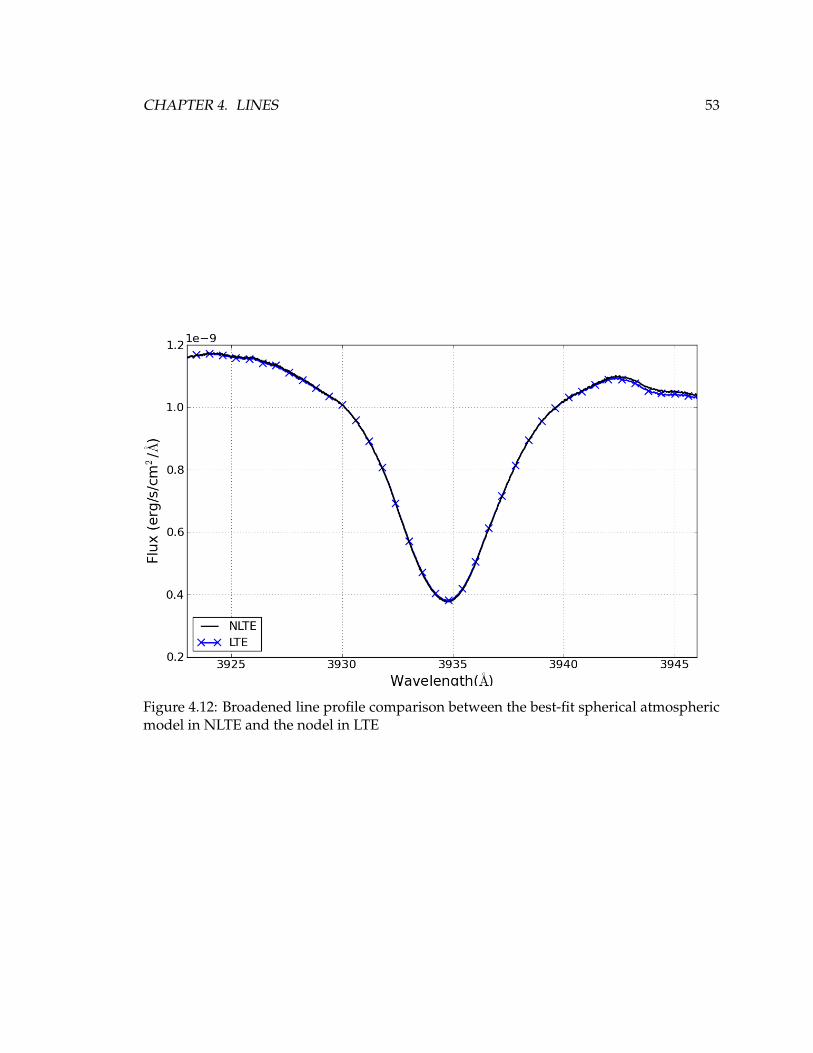
4.12 Broadened line profile comparison between the best-fit spherical atmospheric
model in NLTE and the nodel in LTE . . . . . . . . . . . . . . . . . . . . . . . 53
List of Tables
1.1 Observed properties of αOph . . . . . . . . . . . . . . . . . . . . . . . . . . . 13
2.1 Species treated in NLTE . . . . . . . . . . . . . . . . . . . . . . . . . . . . . . 20
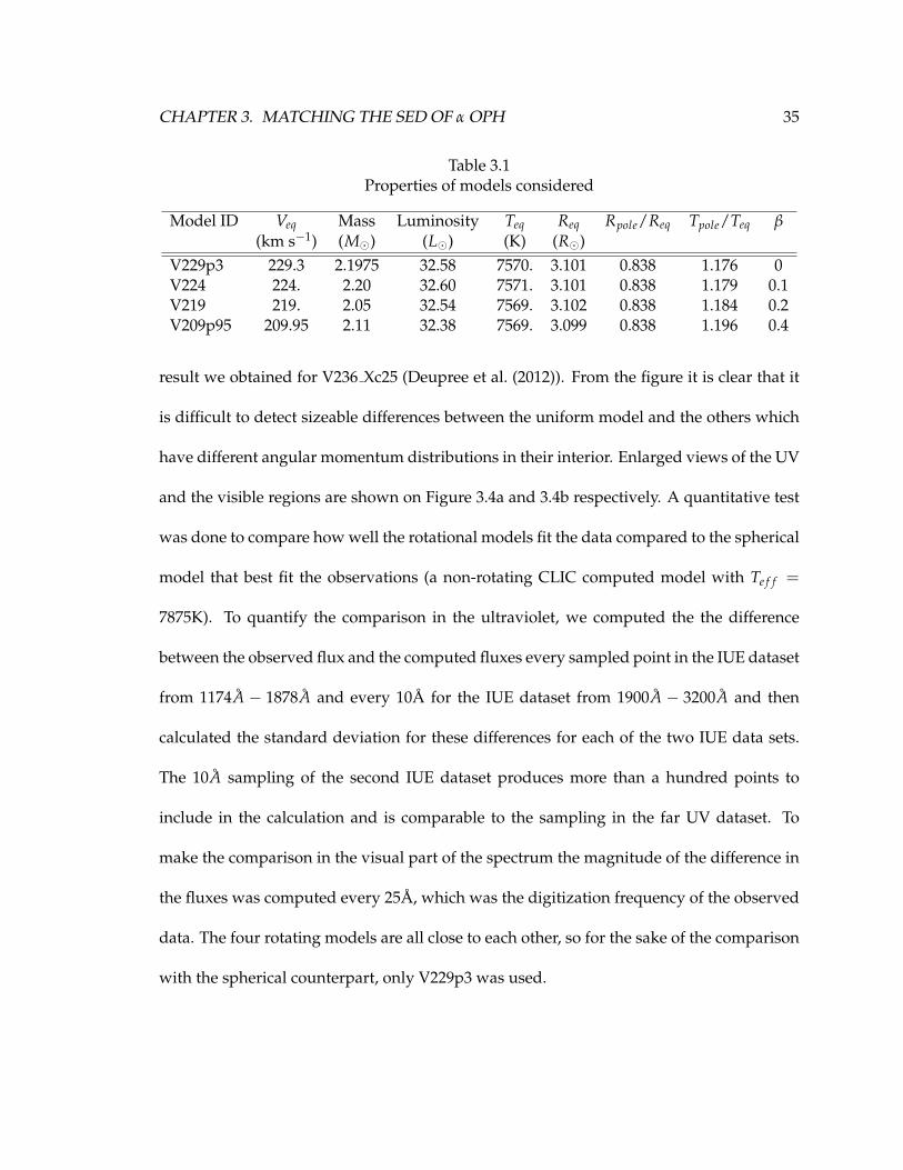
3.1 Properties of models considered . . . . . . . . . . . . . . . . . . . . . . . . . 35
4.1 Properties of ultraviolet lines considered . . . . . . . . . . . . . . . . . . . . . 46
4.2 Properties of visual lines considered . . . . . . . . . . . . . . . . . . . . . . . 47
vii
Abstract
The Effects of Differential Rotation on the Spectral Energy
Distribution and Line Profiles for Models of the Rapidly Rotating
Star α Oph
by Diego Castaneda
The spectrum of the rapidly rotating star α Oph was modeled to examine the effect dif-ferential rotation has on its observed SED. Rotating stellar structure models were generatedusing the code ROTORC and constrained by the star’s interferometrically inferred param-eters. The integrator code CLIC was used to calculate the SED of each model with an NLTEatmosphere (generated by the PHOENIX code) as it would be viewed at the inclination ofα Oph. Comparison of the resultant synthetic SEDs and observations of the star revealedlittle difference between the goodness of fits of models with different rotation profiles dueto the star’s inclination. Higher quality observations are necessary to further constrain thephysical parameters and angular momentum distribution of α Oph but other previouslyobserved rapidly rotating stars are current candidates for study with this technique.
December 18, 2012
1
Chapter 1
Introduction
1.1 Background
Significant advances in the understanding of stellar interiors and evolution have been
made in the last century by increasingly refined observations and by the increase in avail-
able computational resources to solve numerically the equations that describe the physics
inside stars. Most of this research, however, has focused on spherical stars. The most com-
mon case of nonspherical stars is rapidly rotating stars with sufficiently large centrifugal
forces to distort considerably the surface of the star. Sufficiently large rotation generates
hydrodynamic and thermal instabilities in the interior of the star that may change its com-
position and rotation profiles and hence change a star’s properties and evolution. Rapid
rotation can change considerably the physically relevant properties of a star deduced from
the colors and line profiles observed. HR diagrams, masses, lifetimes and other deduced
parameters derived from the assumption of spherical symmetry (implying isotropic flux
1
CHAPTER 1. INTRODUCTION 2
coming out of the star) need to be revised to include the angle dependence at which the
star is being observed.
In order to detect if a star is rotating and how fast if so, one must analyze its individual
spectral lines. The line profiles will be broadened by the Doppler effect as parts of the sur-
face move towards or away from the observer with respect to the center of mass of the star.
A comparison between this line profile and an unbroadened one will reveal the rotation
rate at which we observe the star rotating. One must be careful to take into account that
this velocity observed depends on the inclination (i) with respect to the axis of rotation at
which the star is being observed (i = 0◦ represents the pole-on view and i = 90◦ represents
the equator-on view), which is unknown and cannot be easily deduced from the line pro-
file; this observed velocity is then usually expressed as v sin i. It is known that early type
stars are often fast rotators with values of v sin i as high 400 km s−1 (Abt et al. 2002). This is
a significant fraction of critical rotation, at which the surface equatorial velocity is such that
the centrifugal force equals with the gravitational force. One particular problem for very
rapidly rotating stars is that the lines become so broad and shallow that it becomes very
difficult to distinguish the presence of a line at all, as can be understood by recognizing
that rotation does not change the equivalent width of the line.
Another important factor that will modify the line profile is the angular momentum
distribution on the visible surface of the star. Most early studies considered only solid
body rotation (Ostriker & Mark 1968; Faulkner et al. 1968; Kippenhahn et al. 1970), but
there is currently a fairly high interest in differential rotation (Jackson et al. 2004; Lovekin
2005). While differential rotation refers to any non constant rotation profile, we will be
CHAPTER 1. INTRODUCTION 3
most interested here in a regime in which the angular velocity varies with distance from the
rotation axis. (Gillich 2007) searched for consequences of these different rotation profiles
in the stellar spectrum, both in the broad band spectral energy distribution (SED) and in
the individual line profiles. There are noticeable differences when significant differential
rotation is compared to the solid body case but determining which law describes better
what is observed from a rotating star will depend greatly on the quality of the observations
made for the star in question.
Over the last decade important advances towards improving our knowledge of the
internal structure of rotating stars have been made by combining new interferometric ob-
servations and asteroseismic studies of some known fast rotators. Interferometry has im-
proved to a point in which it is possible to resolve the deformed stellar disk of a star de-
formed by rapid rotation (van Belle et al. 2001, Domiciano de Souza et al. 2003, Aufdenberg
et al. 2006, McAlister et al. 2005, Zhao et al. 2009). These studies have constrained impor-
tant surface parameters like the value the effective temperature and the surface radius at
the pole and at the equator. Finding the actual inclination angle at which the star is being
observed is also possible with high precision (| ∆i |≈ 1◦). For rotating stars two useful
quantities can give insight on how fast is a star rotating: the radius ratio between the pole
and the equator, Rpole/Req, and the difference between the temperature at the pole and
temperature at the equator, Tpole − Teq. Regulus, a rapidly rotating star relatively close to
critical rotation and thought to be rotating at about 336 km s−1, has a ratio between the
polar radius and the equatorial radius of ∼ 0.7 and Tpole − Teq = 3500K (Che et al. 2011).
CHAPTER 1. INTRODUCTION 4
1.1.1 Modelling Rotating Stars
In the interior of a rotating star centrifugal forces reduce the effective gravity depending
on the latitude and also introduce deviations from sphericity. If such stars are to be mod-
eled, the four equations of stellar structure need to be modified, and introducing all the
effects imposed by rotation into the calculation of realistic models that can be compared
to observations have been quite a challenge for several decades. Several approximations
has been made trying to simplify the problem; the most famous approximation still used
today is known as von Zeipel’s law (1924). He showed that uniformly rotating models
have the state properties constant on equipotential surfaces, and under the condition of
radiative equilibrium, the star has a local surface flux that is proportional to the local grav-
ity, F ∝ g. Using the Stefan-Boltzmann law, where F = σT4e f f , von Zeipel’s law implies
that Te f f ∝ g0.25. Actual observation and application of this relation however, indicate that
slightly different exponents of the gravity appear to provide a better match to the deduced
properties, so a general parametrization of the relationship between the effective tempera-
ture and the gravity is often used: Te f f ∝ gβ (Lucy 1967; Kippenhahn 1977; Maeder 1999).
This relation is a common tool used to simplify the calculation of the surface properties
of a rotating star where the potential, assuming the Roche potential for the gravitational
potential, can be expressed as
Φ =GMR(θ)
+12
ω2R(θ)2sin2θ = constant. (1.1)
For this potential, the two components of the effective gravity in polar coordinates can
CHAPTER 1. INTRODUCTION 5
be easily found to be,
gr(θ) = −dΦdr
= − GMR(θ)2 + ω2R(θ)sin2θ (1.2)
and
gθ(θ) = −1r
dΦdθ
= R(θ)ω2sinθcosθ. (1.3)
Here G is the gravitational constant, M is the mass, ω is the angular velocity and θ is
the colatitude. The magnitude of the effective gravity at any latitude θ can be calculated
from ge f f =√
g2r + g2
θ (Aufdenberg et al. 2006) and finally from von Zeipel’s law one can
find the effective temperature for any given latitude.
There are, however, several shortcomings with the method described by von Zeipel.
The assumption of a stellar surface that can be described with a Roche potential only holds
for stars whose density distribution in the deep interior is not perturbed from a spherical
distribution. Such stars include all uniform rotating cases except those rotating exceed-
ingly close to critical rotation (Lovekin et al. 2006). Moderately and rapidly rotating stars
with rotation rates increasing with decreasing distance from the rotation axis can not be
described by a Roche potential and the actual gravitational potential must be calculated.
Equation 1.1 does not hold for non-conservative rotation laws because in that case there
is no such thing as a potential by definition. One other concern with von Zeipel’s law is
the decoupling of the effective temperature and the surface temperature. The von Zeipel’s
theorem assumes that the temperature is constant along an equipotential surface, includ-
CHAPTER 1. INTRODUCTION 6
ing the stellar surface, while in an actual rotating star the effective temperature is varying
from pole to equator.
Von Zeipel’s result in which the state variables are constant on equipotential surfaces
led to the development of two computational approaches for calculating rotating stellar
models in the late 1960’s. One of these approaches, the self-consistent field method (Os-
triker & Mark 1968), solved for the gravitational potential for a given density distribution
and then solved for a new density distribution on equipotential surfaces from hydrostatic
equilibrium. The new densities led to a new approximation of the gravitational poten-
tial, and the entire process was iterated until all changes were sufficiently small. Jackson
(1970) modified this method to include thermal equilibrium as well and has computed a
number of rapidly rotating stellar models (Jackson et al. 2004,2005; MacGregor et al. 2007).
Bodenheimer (1971) also used the method to compute a number of rapidly rotating main-
sequence models for several angular momentum distributions. Clement (1974; 1978; 1979)
modified the original double series expansion for the gravitational potential with a two-
dimensional (2D) finite-difference approach.
The second approach, developed by Monaghan & Roxburgh (1965) and extended and
utilized by others (e.g., Roxburgh et al. 1965; Faulkner et al. 1968; Kippenhahn & Thomas
1970; Sackmann & Anand 1970), allowed certain rotating models to be calculated in a one-
dimensional (1D) framework. This approach was extended by Endal & Sofia (1976; 1978) to
include the redistribution of angular momentum in this 1D framework for a number of hy-
drodynamic and thermal instabilities, and such prescriptions are now commonly included
in stellar evolution codes (e.g., Demarque et al. 2007; Eggenberger et al. 2007).
CHAPTER 1. INTRODUCTION 7
An alternative to these methods is to solve for all of the appropriate equations and
their boundary conditions simultaneously on a 2D grid (e.g. Clement 1978,1979; Deupree
1990,1995; Espinosa Lara 2010). The reason for using this framework was to include the ap-
propriate velocity terms in the conservation equations to compute features such as merid-
ional circulation. However, it can also be used to calculate the stellar structure of isolated
models as well as members of evolution sequences.
After the stellar structure is obtained, the surface values of these models can be used
as input to construct an appropriate emergent flux that includes the effects of the surface
variation of the relevant properties of the star. This can be done by performing an integra-
tion over the visible surface of the star of the intensities emerging from many atmosphere
models that are defined by the local surface parameters of the star. Collins (1963) was one
of the first ones to attempt such atmospheric modeling by using von Zeipel’s law, uniform
rotation and grey atmospheres where the radiative transfer equation was greatly simpli-
fied. One of the most significant conclusions from his work was how much the observed
luminosity of a rotating star depended on the angle at which it was observed. Later re-
finements using various atmospheric models to describe a single rotating star confirmed
those early results (e.g., Collins et al. 1991; Collins & Truax 1995). More improvements
would come from the level of realism included in the atmosphere modeling. Maeder &
Peytremann (1970) computed LTE atmospheres where the hydrogen line opacities for the
Balmer and Lyman series were included. Slettebak et al. (1980) and Fremat et al. (2005)
added more realism by using a series of non-LTE atmospheres in their models.
The next step after a satisfactory atmospheric model is achieved is to determine observ-
CHAPTER 1. INTRODUCTION 8
able properties from this synthetic set up. In general, a model atmosphere will produce the
intensity emerging from the atmosphere as a function of the direction with respect to the
local surface normal. If one takes the component of each set of rays in the direction of the
observer, it is possible to determine the flux at each wavelength that will be observed at
some distance from the star. The general expression for this integration in spherical coor-
dinates would be:
Fλ(i) =ˆ
θ
ˆφ
Iλ′(ξ(θ, φ, i))W(λ, λ′)dAprojcos ξ(θ, φ, i)
d2 , (1.4)
where ξ is the angle between the local normal to the surface and the direction to the ob-
server, W(λ, λ′) denotes the wavelength change produced by the Doppler shift, and the
element of projected area, dAproj, is given by
dAproj = R2(θ)sin θ cos ξ
√1 +
(dRdθ
)2 1R2 dθdφ. (1.5)
This flux will provide the spectral energy distribution (SED), and from the SED quan-
tities like the observed luminosity and the colors in any band can be calculated. For a
rotating star the same principle applies, but there would be a dependency between all the
observable quantities and the angle with respect to the rotation axis at which the obser-
vation is set to be made. This whole procedure can become difficult and highly computer
intensive, so as expected, approximations have been made to ease the reproduction of such
observables. The most important is known as the limb darkening law (Carroll 1928, 1933;
Shajn & Struve 1929), in which the star is treated as a circular disk in which the edges of
CHAPTER 1. INTRODUCTION 9
the disk or “limbs” will contribute less intensity to the total flux, hence the “darkening” on
those zones. Slettebak (1949) applied this idea to rotating stellar models where the defor-
mation at the equator will reduce the effective gravity, and recalling von Zeipel’s theorem,
this will reduce the flux coming out of this area, producing an equivalent effect to the limb
darkening similarly called gravitational darkening. In the end, one would expect that the
method in which the actual intensities coming out of each zone in the atmosphere of the
star are integrated would produce more realistic results. Both the limb darkening and the
gravitational darkening are automatically incorporated in this calculation without any re-
strictive assumptions.
The final test of all the effort put into the modeling of these stars comes from compar-
ison with real known rotating stars. Stellar rotation studies have struggled here because
the only measurable trace of rotation in a stellar spectrum was v sin i. That left a large
set of unknowns only very weakly constrained within the models, and great levels of de-
generacy on parameters such as the inclination, Req and Rpole, Te f f at the equator and the
pole, the internal angular momentum distribution, among others. Fortunately, in the last
decade, great advances in instrumentation have allowed asteroseismology and optical in-
terferometry to provide the determination or constraint of many of these free parameters.
Asteroseismology provides a good test for the internal structure of the star, while interfer-
ometry is allowing direct resolved observations of deformed rotating stars, providing their
inclination and their oblateness. Good candidates have surfaced such as the rapidly rotat-
ing star Achenar (Domiciano de Souza et al. 2003) but this early attempt was clouded by
the possibility that a circumstellar envelope was contributing to the oblateness measured
CHAPTER 1. INTRODUCTION 10
by the interferometry as well as the stellar surface (Vinicius et al. 2006; Kanaan et al. 2008;
Carciofi et al. 2008; Kervella et al. 2009). It was possible to successfully reproduce the ob-
served shape (Jackson et al. 2004) but only with a markedly differentially rotating model.
Several various other rapidly rotating stars have now been successfully resolved by inter-
ferometry. One of these stars, α Oph, will be the focus of this work as it has proven to be
great test case to model for reasons that will be discussed in the next section.
1.2 α Oph
The search for a good candidate to test current stellar interior structure models that include
rotation led us to the brightest star in the constellation of Ophiuchius. α Oph itself is a
binary system with an extremely eccentric orbit of e = 0.92 ± 0.03 (Hinkley et al. 2011)
and a period of 8.62 years. An interesting fact is that the companion, a K2 V star, makes a
very close approach (∼ 0.50AU) at periastron. Also of interest is that the orbital plane (i =
125◦± 8◦) is not aligned with the rotational equator of the main star. In this work the binary
nature of α Oph is not relevant, but the dynamical evolution of the star (particularly its
angular momentum history) may have influenced the properties of the principal member
in the binary system. It is also important to note that the dwarf companion contributes
only an estimated 1.2% of the observed flux in the red (van de Kamp 1967). For notation
purposes we will refer to the primary, the one we’re interested in, of the system as simply
α Oph. Classified as an A5IV δ Scuti star, α Oph (=HR 6556, HD 159561) is the seventh
brightest A-type star in the sky and has an observed Veq sin(i) of about 240 km s−1 (Royer
CHAPTER 1. INTRODUCTION 11
et al. 2002). This is sufficiently large for the rotation to have appreciable effects on at least
the surface conditions.
It was observed interferometrically with the CHARA array by Zhao et al. (2009) and
asteroseismologically with the MOST satellite (Monnier et al. (2010)). The interferometry
revealed that α Oph is seen nearly equator on, with a ratio of the polar radius to the equato-
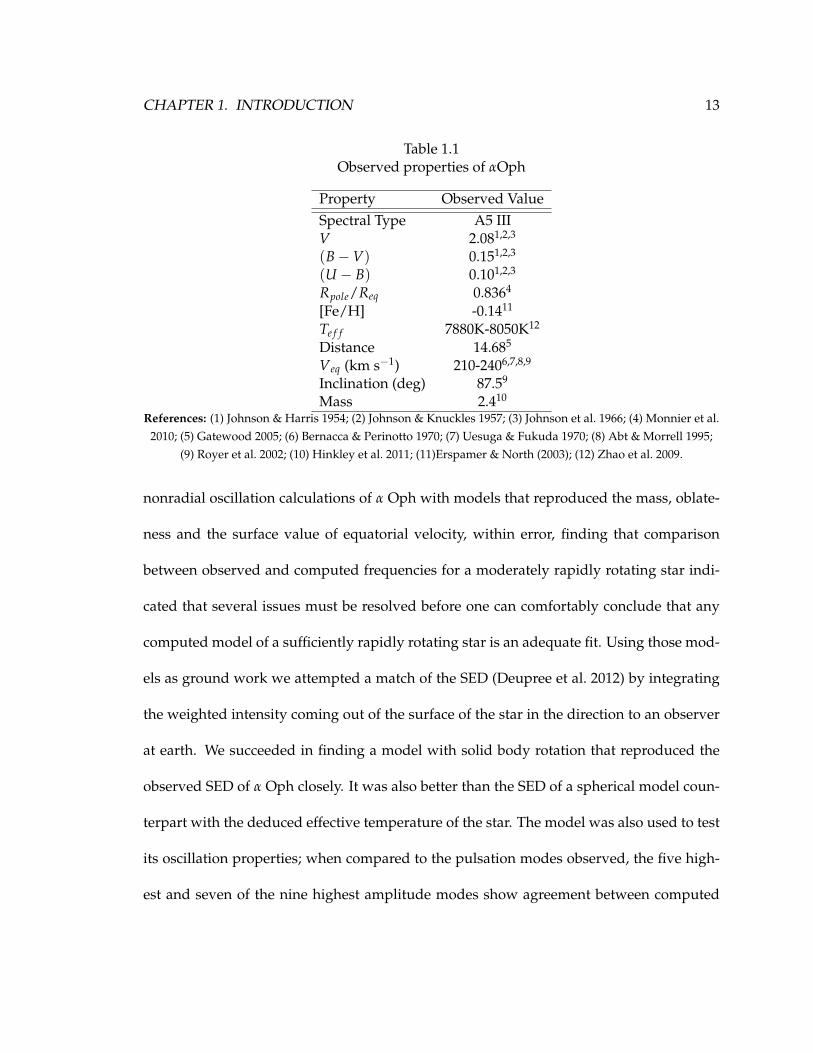
rial radius of about 0.836. A summary of the key observed properties is given in Table 1.1.
An important note to the observed properties is that the deduced mass was derived from
the orbital solution of the binary system, which provides a more fundamental and accurate
measurement than a mass estimated by its location in the HR diagram. The observed lumi-
nosity and effective temperature (i.e., those quantities deduced assuming that the observed
flux is produced by a spherical star) range from 7880 to 8050K for the effective temperature
and from 25.1 to 25.6 L� for the luminosity (Blackwell & Lynas-Gray (1998); Malagnini &
Morossi (1990); Monnier et al. (2010)). These values should be quite accurate given that
the star has a well-determined parallax (see discussion in Gatewood (2005)), and there is
insignificant reddening. These results also place the star relatively close to the blue edge of
the instability strip (e.g., Breger 2000; Xu et al. 2002). However, the perceived effective tem-
perature and luminosity depend on the inclination between the observer and the rotation
axis, and the actual luminosity and effective temperature for a rapidly rotating model seen
equator on will both be higher than perceived, possibly placing α Oph even closer to the
blue edge. One desirable consequence of this is that atmospheric convection is likely not
significant and can be ignored. The combination of the deduced luminosity, effective tem-
peratures at the pole and the equator, the observed oblateness, surface equatorial velocity
CHAPTER 1. INTRODUCTION 12
and inclination, limit even more the possible models for this star.
To determine the precise relationship between those observed properties and the actual
ones requires the calculation of the spectral energy distributions which can be compared
with observations of α Oph. Instead of applying the often used limb and gravity dark-
ening assumptions to calculate the SED (e.g., Claret 2003; Reiners 2003; Townsend et al.
2004; Monnier et al. 2010), a more rigorous approach would be to integrate the weighted
intensity coming out of the star in the direction of the observer over all the visible surface
using the latitudinal variation of the radius, the local effective gravity and the local effec-
tive temperature to obtain the observed flux (e.g., Slettebak et al. 1980; Linnell & Hubeny
1994; Fremat et al. 2005; Gillich et al. 2008). Rotating models whose properties match the
observed spectral energy distribution, the surface equatorial velocity, and the oblateness
would appreciably confine at least the surface stellar rotation properties. The other key
component available in this case is the ability to check how well the internal structure mod-
els match the pulsation modes observed. Analysis of the MOST data for α Oph revealed
57 oscillation frequencies which clearly must include both p and g modes. The combi-
nation of the comparatively large number of oscillation modes and the relatively detailed
knowledge about the stellar properties make α Oph a good candidate to explore specific
problems that might be encountered when trying to match the entire collection of data. It is
important to note that none of the oscillation frequencies has a half amplitude larger than
0.7 mmag, so that we do not have to be concerned about the variation of the atmospheric
properties with pulsation phase in simulations of the SED or the spectral lines.
Deupree (2011) performed both 2D stellar evolution simulations and linear, adiabatic,
CHAPTER 1. INTRODUCTION 13
Table 1.1Observed properties of αOph
Property Observed ValueSpectral Type A5 IIIV 2.081,2,3
(B−V) 0.151,2,3
(U − B) 0.101,2,3
Rpole/Req 0.8364
[Fe/H] -0.1411
Te f f 7880K-8050K12
Distance 14.685
Veq (km s−1) 210-2406,7,8,9
Inclination (deg) 87.59
Mass 2.410
References: (1) Johnson & Harris 1954; (2) Johnson & Knuckles 1957; (3) Johnson et al. 1966; (4) Monnier et al.2010; (5) Gatewood 2005; (6) Bernacca & Perinotto 1970; (7) Uesuga & Fukuda 1970; (8) Abt & Morrell 1995;
(9) Royer et al. 2002; (10) Hinkley et al. 2011; (11)Erspamer & North (2003); (12) Zhao et al. 2009.
nonradial oscillation calculations of α Oph with models that reproduced the mass, oblate-
ness and the surface value of equatorial velocity, within error, finding that comparison
between observed and computed frequencies for a moderately rapidly rotating star indi-
cated that several issues must be resolved before one can comfortably conclude that any
computed model of a sufficiently rapidly rotating star is an adequate fit. Using those mod-
els as ground work we attempted a match of the SED (Deupree et al. 2012) by integrating
the weighted intensity coming out of the surface of the star in the direction to an observer
at earth. We succeeded in finding a model with solid body rotation that reproduced the
observed SED of α Oph closely. It was also better than the SED of a spherical model coun-
terpart with the deduced effective temperature of the star. The model was also used to test
its oscillation properties; when compared to the pulsation modes observed, the five high-
est and seven of the nine highest amplitude modes show agreement between computed
CHAPTER 1. INTRODUCTION 14
axisymmetric, equatorially symmetric mode frequencies within the observational error. In-
cluding nonaxisymmetric modes up through |m| = 2, and allowing for the possibility that
the eight lowest amplitude modes could be produced by modes that are not equatorially
symmetric, it matched 24 out of the 35 MOST modes to within the observational error.
Based on a comparison of these frequency results with those of Deupree (2011), it is
clear that being able to match the observed SED in both the visual and ultraviolet plays a
crucial role in constraining the model but still issues remain. The most important of these
is perhaps the internal angular momentum distribution. It is clear that the model repro-
duced the surface values closely with uniform rotation, leading to the expectation that the
star may not be too far from uniform rotation, at least near the surface. This assumes that
the surface is an equipotential, something that, while not unreasonable, remains an as-
sumption. One would expect for a star as evolved as α Oph that a more reasonable angular
momentum distribution would not correspond to a conservative rotation law because at
least part of the core would be rotating more quickly than the surface, even at the pole, in
which case no equipotential can be defined. The next natural step in the investigation is
to test different models that have non uniform internal angular momentum distributions,
which is the intention of the present work. The next chapter present the steps in the calcu-
lation procedure, same as the one used in Deupree et al. (2012), to obtain the SEDs of those
models.
Chapter 2
Methods
2.1 The synthetic SED of a rotating star
In order to compute observable quantities other than the total luminosity of a rotating star,
it is not enough to just model its possible interior structure. All the radiation we observe
or measure from any star comes from its atmosphere, and although the internal structure
will set up the conditions of such an atmosphere, a good model is necessary to succeed
in creating a realistic spectrum. The SED is one of those observables that require a good
atmosphere calculation, and when stellar rotation is included, this atmosphere model must
take into account all the effects that a rotating star has with its latitudinally varying surface
parameters. Various SEDs were calculated for comparison to observations of α Oph. A
detailed procedure of how they were obtained is presented below.
The methodology used is based on the work of Lovekin et al. (2006) and Gillich et al.
(2008) which consists of 3 steps to obtain the spectra: The first is the calculation with RO-
15
CHAPTER 2. METHODS 16
TORC of a fully 2D stellar evolution model that includes rotation (Deupree 1990; 1995;
1998). This model will provide the surface values of effective temperature and effective
gravity at each point on the surface of the deformed star. The second step is the calculation
of plane parallel atmospheres with the PHOENIX model atmospheric code. The variation
of temperature and gravity with the colatitude of the star requires the computation of a
whole grid of different atmospheric models that will cover all the possible values of tem-
perature and gravity given by the ROTORC model. The assumption is that the emergent
intensity at any point on the surface can be approximated as that for a plane parallel model
atmosphere with the local effective temperature and surface gravity. Using various plane
parallel atmospheres is a good approximation in this case because any significant horizon-
tal variation is apparent only over many photon mean free paths, and the radial extent of
the atmosphere is very small in comparison to the stellar radius. The actual atmosphere
of the rotating stellar model will be generated from the atmosphere grid by interpolating
the intensity rays emerging from the surface of each plane-parallel PHOENIX model as
a function of angle from the normal to the surface. In the last step, CLIC, a code devel-
oped by Lovekin et al. (2006), will be used to perform the numerical integration of these
intensities over the observed surface of the star to obtain the SED one would observe at a
user-specified distance and inclination with respect to the axis of rotation of the star. Each
component of the modeling process is detailed in the next sections.
CHAPTER 2. METHODS 17
2.1.1 ROTORC
ROTORC is a fully implicit 2D hydrodynamics and hydrostatics stellar evolution code de-
veloped by Deupree (1990,1995) to determine the structure of rotating stellar models. In
this context, ROTORC provides the effective temperature, effective gravity, radius, and ro-
tational velocity at the surface as a function of latitude. There are no specific requirements
about the angular momentum distribution, although the surface location at each latitude
is found as if the surface were an equipotential. Time-dependent equations of momentum,
thermal balance, along with Poisson’s equation, the equation of state, and relations for the
nuclear energy generation and the radiative opacity are solved simultaneously for the den-
sity, pressure, temperature, velocity in three dimensions and gravitational potential at each
location in a 2D grid. It should be noted that ROTORC does not assume a Roche potential.
ROTORC was used in a mode where the rotational velocities can be imposed through a
rotation law and the velocities in the radial and latitudinal direction reflect only the stellar
evolution. The method of solution is a two-dimensionalization of the Henyey technique
outlined by Deupree (1990). In this method, for each zone in the grid, a first guess for all
of the unknown variables is made and the difference equations are expressed as first-order
expansions in corrections to all the unknown variables. Then, by the equivalent of a ma-
trix inversion, a simultaneous solution for all the first order corrections is found, giving a
second approximation to the actual solution. The process is iterated until the corrections
are considered to be small enough and the result can be used as an initial guess for the
next time step in the evolutionary sequence. Since all equations, boundary conditions and
CHAPTER 2. METHODS 18
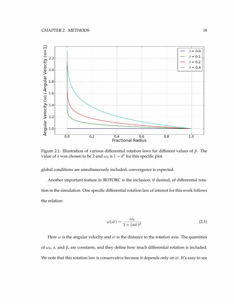
Figure 2.1: Illustration of various differential rotation laws for different values of β. Thevalue of a was chosen to be 2 and ω0 is 1 + aβ for this specific plot.
global conditions are simultaneously included, convergence is expected.
Another important feature in ROTORC is the inclusion, if desired, of differential rota-
tion in the simulation. One specific differential rotation law of interest for this work follows
the relation:
ω(v) =ω0
1 + (av)β(2.1)
Here ω is the angular velocity and v is the distance to the rotation axis. The quantities
of ω0, a, and β, are constants, and they define how much differential rotation is included.
We note that this rotation law is conservative because it depends only on v. It’s easy to see
CHAPTER 2. METHODS 19
from equation 2.1 that solid body rotation is recovered when β = 0. Figure 2.1 shows the
different rotation laws that will be considered in this work.
2.1.2 PHOENIX
PHOENIX (Hauschildt & Baron 1999) is a non-LTE stellar atmosphere and spectrum syn-
thesis code that generates (for our purposes) 1D plane-parallel models by solving the equa-
tions of hydrostatic equilibrium, thermal equilibrium, equations of state and the equation
of radiative transfer:
dIλ
dτλ= Iλ −
jλκλ
, (2.2)
where τλ is the optical depth at the specific wavelength λ. The ratio of the emission and
absorption coefficients, jλ and κλ, is known as the source function S(λ).
PHOENIX is commonly used in a two step process in which initially a stellar structure
model of the atmosphere is converged, and finally, the code finds the formal solution of the
radiative transfer equation to synthesize a spectrum.
The code is capable of keeping track of the population of thousands of atomic energy
levels, and the calculation can be performed under two different regimes:
local thermodynamic equilibrium (LTE) or non-LTE (NLTE). LTE assumes equilibrium be-
tween matter and the local radiation field, with the electron population of atomic energy
levels described by Boltzmann statistics, the ionization equilibrium by the Saha equation,
and the source function of the radiation field, Sλ, by the Planck function Bλ(T). However,
CHAPTER 2. METHODS 20
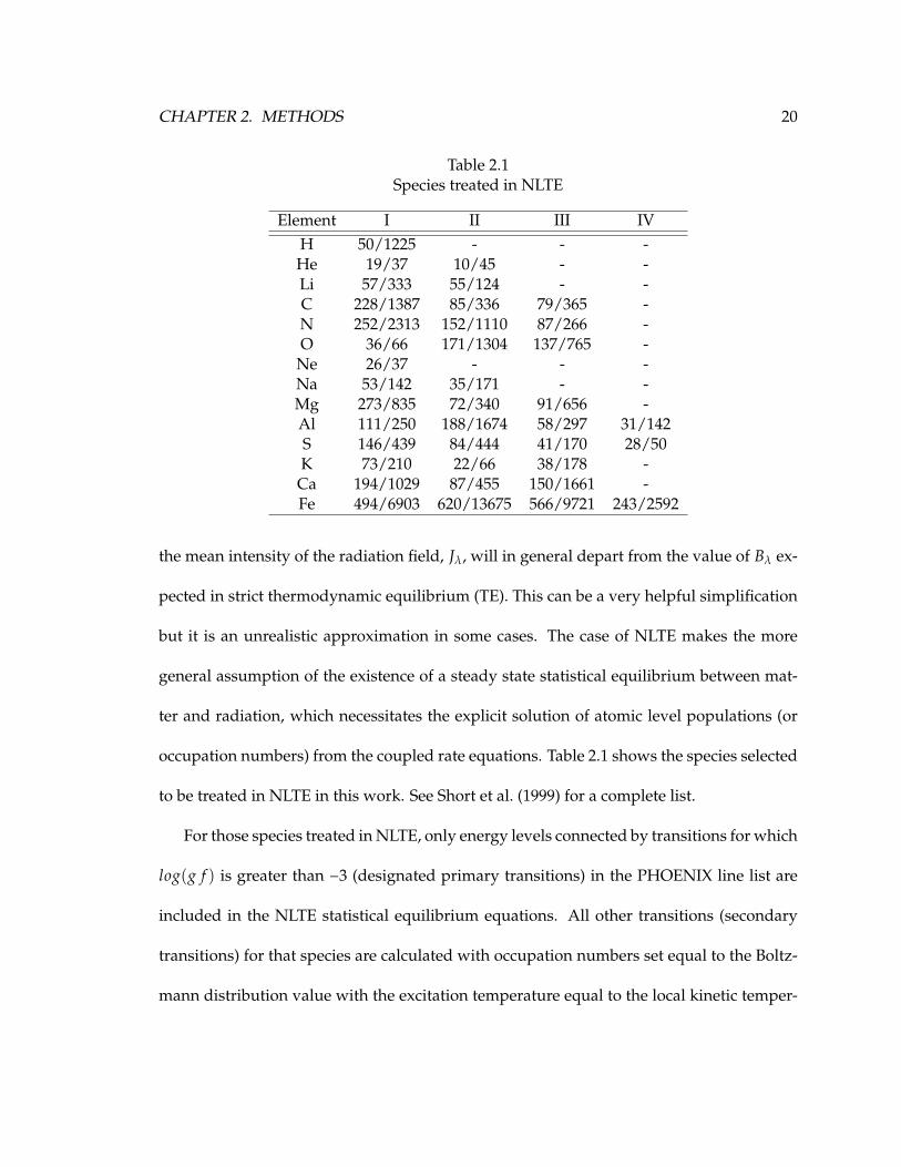
Table 2.1Species treated in NLTE
Element I II III IVH 50/1225 - - -He 19/37 10/45 - -Li 57/333 55/124 - -C 228/1387 85/336 79/365 -N 252/2313 152/1110 87/266 -O 36/66 171/1304 137/765 -
Ne 26/37 - - -Na 53/142 35/171 - -Mg 273/835 72/340 91/656 -Al 111/250 188/1674 58/297 31/142S 146/439 84/444 41/170 28/50K 73/210 22/66 38/178 -Ca 194/1029 87/455 150/1661 -Fe 494/6903 620/13675 566/9721 243/2592
the mean intensity of the radiation field, Jλ, will in general depart from the value of Bλ ex-
pected in strict thermodynamic equilibrium (TE). This can be a very helpful simplification
but it is an unrealistic approximation in some cases. The case of NLTE makes the more
general assumption of the existence of a steady state statistical equilibrium between mat-
ter and radiation, which necessitates the explicit solution of atomic level populations (or
occupation numbers) from the coupled rate equations. Table 2.1 shows the species selected
to be treated in NLTE in this work. See Short et al. (1999) for a complete list.
For those species treated in NLTE, only energy levels connected by transitions for which
log(g f ) is greater than −3 (designated primary transitions) in the PHOENIX line list are
included in the NLTE statistical equilibrium equations. All other transitions (secondary
transitions) for that species are calculated with occupation numbers set equal to the Boltz-
mann distribution value with the excitation temperature equal to the local kinetic temper-
CHAPTER 2. METHODS 21
ature, multiplied by the NLTE departure coefficient for the ground state in the next higher
ionization stage.
The energy level and bound–bound transition atomic data have been taken from Ku-
rucz (1994) and Kurucz & Bell (1995). The resonance-averaged Opacity Project (Seaton
et al. (1994)) data of Bautista et al. (1998) have been used for the ground-state photoion-
ization cross sections of Li (I–II), C (I–IV), N (I–VI), O (I–VI), Ne (I), Na (I–VI), Al (I–VI),
Si (I–VI), S (I–VI), Ca (I–VII), and Fe (I–VI). For the ground states of all stages of Mg, P,
Ti and for the excited states of all species, the cross-sectional data previously incorporated
into PHOENIX from either Reilman & Manson (1979) or from the compilation of Mathisen
(1984) was used. The coupling among all bound levels by electronic collisions is calculated
using cross sections calculated from the formulae compiled by Allen (1973). The cross sec-
tions of ionizing collisions with electrons are calculated from the formula of Drawin (1961).
2.1.3 CLIC
The intensity integrator code, developed by Lovekin et al. (2006) and later modified and
used by Gillich et al. (2008), is a tool for calculating the SED of a rotating star model. It
computes as a function of wavelength the flux an observer would measure outside Earth’s
atmosphere for a star at a specified distance. As input, CLIC needs the surface properties
of the stellar model of interest: radius, effective temperature (Te f f ), the logarithm of the
effective gravity (log(g)) and the rotational velocity as function of colatitude. These are
are provided by ROTORC. To model the atmosphere of the star the whole non spherical
surface is divided into a mesh of 200 zones in θ and 400 zones in φ in which the intensities
CHAPTER 2. METHODS 22
emerging from each piece of stellar surface of the star in the direction of the observer,
Iλ(ξ(θ, φ, i)), are obtained from interpolation through the grid of the appropriate plane-
parallel model atmospheres generated by PHOENIX. Including the entire surface allows
the flux the observer would see to be determined at any arbitrary inclination.
The observed flux is then calculated as a weighted integral of those intensities coming
out of each zone over the visible surface of the star (equation 1.4). The visible surface will
depend on the inclination with respect to the local vertical direction of the star at which the
surface is being observed. The integral is calculated for each wavelength with a separation
∆λ = 0.02A, which provided a good sampling of the line profiles, especially in the UV.
This wavelength separation is also better than the resolution of the data to be discussed
later. The geometry of the problem is fully described by Lovekin et al. (2006).
The program is set up to output ten different fluxes corresponding to ten different ob-
served inclinations with respect to the star pole, starting with i = 0◦ (pole on view) to
i = 90◦ (equator on view) in 10 uniform steps. An example of the different SEDs ob-
tained for a model with Veq = 233 km/s and mass of 2.2M� as a function of inclination
with respect to the star’s vertical is shown in Figure 2.2. The code can be easily modified
to compute the observed flux for any desired inclination. In our case, we set up CLIC to
compute the flux at the deduced inclination of α Oph, 87.5◦.
The SED is intended to cover a large part of the spectrum, usually with flux averages
computed after that, so broadening effects on individual lines are not considered. This
allows the decoupling of individual wavelengths, making the calculation ideal for parallel
processing. When considering small regions of the spectrum, CLIC has a subroutine that
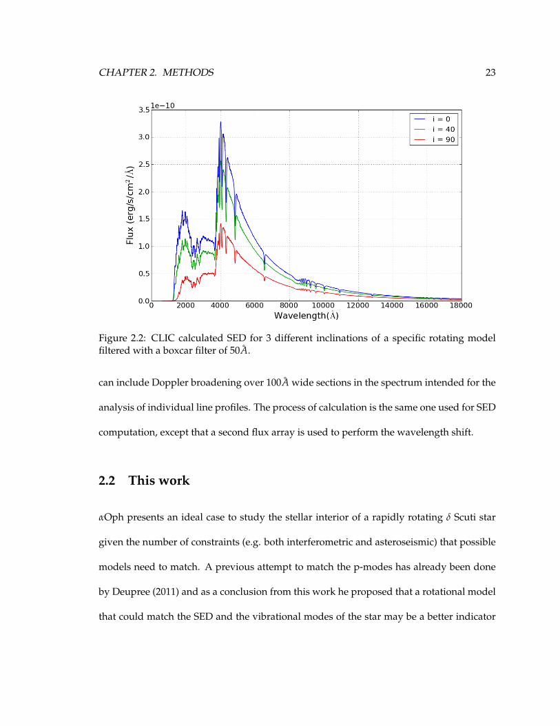
CHAPTER 2. METHODS 23
Figure 2.2: CLIC calculated SED for 3 different inclinations of a specific rotating modelfiltered with a boxcar filter of 50A.
can include Doppler broadening over 100A wide sections in the spectrum intended for the
analysis of individual line profiles. The process of calculation is the same one used for SED
computation, except that a second flux array is used to perform the wavelength shift.
2.2 This work
αOph presents an ideal case to study the stellar interior of a rapidly rotating δ Scuti star
given the number of constraints (e.g. both interferometric and asteroseismic) that possible
models need to match. A previous attempt to match the p-modes has already been done
by Deupree (2011) and as a conclusion from this work he proposed that a rotational model
that could match the SED and the vibrational modes of the star may be a better indicator
CHAPTER 2. METHODS 24
of the actual internal structure of αOph. As a follow up, we showed that a stellar model
that includes rotation fits the observed properties of the SED better than a simple spherical
non-rotating one (Deupree et al. 2012). This last work considered only solid body rotation,
and as discussed in Section 1.2, for an evolved star like αOph, uniform rotation is probably
unrealistic. We can make a crude estimate of the amount of differential rotation a star like
α Oph in the latter phase of core hydrogen burning would have in the following manner.
We assume that the star was uniformly rotating on the Zero Age Main Sequence and that
it locally conserves angular momentum (except maybe in the convective core) during its
evolution. We then compare the angular momentum distribution along the equator be-
tween the centre and surface of the model with the distributions imposed by equation 2.1
for various values of beta. This distribution resembles that from the equation with β = 0.4
except near the centre, where the angular momentum redistribution by convection makes
any result questionable in any event. This can only be an approximation because we im-
pose a conservative rotation law in a situation for which it is probably false. Nevertheless,
the β = 0.4 rotation case may be a reasonable upper limit to the amount of differential
rotation for this form of the rotation law.
The generation of the synthetic SEDs of αOph follow the recipe described before and
used by Lovekin et al. (2006) and Gillich et al. (2008), using the ROTORC models with
non-uniform internal angular momentum distributions given in equation 2.1. Various pos-
sible 2D internal structure models of α Oph which have the observed oblateness and other
surface parameters were produced to compare with the observed SED when placed at the
proper distance. After comparing the broadband SED we checked the profile of 12 differ-

CHAPTER 2. METHODS 25
ent individual lines and features including the Doppler broadening product of the stellar
rotation. With both the full SED and the lines we test if it is possible to deduce the existence
of differential rotation in the interior of the αOph.
Chapter 3
Matching the SED of α Oph
We calculated a grid of PHOENIX NLTE model atmospheres covering values of Te f f be-
tween 7500K and 9250K in steps of 250K, and for each temperature a range of values of
log(g) between 3.333 and 4.0 with a step of 0.333. All models were calculated with so-
lar composition. As previously mentioned, we need to cover all the surface properties
of the stellar models provided by ROTORC. A typical microturbulence velocity value for
a late A star (Gray et al. 2001) of 2km s−1 was used in each plane parallel model atmo-
sphere. It is important to note that this parameter will not have a great impact on the line
broadening process compared with the broadening effects caused by the rapid rotation
of α Oph. The emergent intensities of these plane parallel atmospheres were calculated
between 600A and 20 000A at a variable step size in wavelength in order to try to keep
a resolution λ/∆λ higher than 200 000, which is sufficient to resolve most features in the
spectrum. The wavelength range selection was done when the integration of the flux be-
tween these wavelengths and the theoretical luminosity given by the Stefan-Boltzmann
26
CHAPTER 3. MATCHING THE SED OF α OPH 27
law for the Te f f for the atmospheric model agreed to within 1%. An important aspect to
note about PHOENIX is that it must automatically “add” wavelength points in between
the specified values of ∆λ if it detects that there is a NLTE spectral line that will be missed
in the current wavelength step. The calculation of each NLTE atmosphere is relatively com-
puter intensive, sometimes needing more than 48 hours of 4 CPUs working in parallel to
converge a a single model.
After finishing the grid, and in conjunction with the ROTORC model of interest, we
used CLIC to obtain the SEDs at ten different inclinations with respect to the line of sight.
The SED is set up to have a ∆λ = 0.02A and is calculated from 1000A to 20 000A which
gives more than enough resolution to critically sample most of the absorption features in
the spectra of α Oph, and also to compute different deduced properties such as the intrin-
sic colors, the observed luminosity and the deduced effective temperature. This starting
wavelength was used for the CLIC synthesis in comparison with the atmospheric model
files after observing that the flux contribution between 600A− 1000A was minimal. The
observed luminosity in this synthetic case will be simply the integral of the SED in the
wavelength range considered, adding the contribution of the Rayleigh-Jeans tail with the
analytical approximation after 20 000A to account for any missing flux beyond our upper
wavelength limit. For the most part we considered a single inclination of the CLIC out-
put file that corresponds to i = 87.5◦, set up to match the observed inclination of α Oph.
Finally, SED fluxes were scaled to reflect the 14.6pc distance of α Oph (Gatewood 2005).
Interstellar extinction can be determined from the color excess of E(B − V) = 0.01mag
(Crawford (2001)). This by itself is a relatively small value, so small that it does not have
CHAPTER 3. MATCHING THE SED OF α OPH 28
many significant digits and may be hard to accurately include. For our models interstellar
extinction was assumed to be zero.
We also want to compare our rotating model SEDs with that for a spherical model
that best fit the SED on the visible part of the spectrum. The effective temperature for the
spherical model was 7875K. The SED for the spherical model was calculated in the same
way as the SEDs for the rotating models.
We examined various observed data sets of α Oph in regions of the visible and ul-
traviolet part of the spectra to compare with the computed SEDs. For the visible re-
gion we used the data set L1985BURN, file 01398 of the HyperLeda catalog (Paturel et al.
(2003)) and based on the spectrometry of Burnashev (1985). SED measurements in the UV
were found from the IUE and OAO2 space observatories for wavelengths between 1200A
and 3000A. The IUE data considered came from sets SWP17411 (1150A − 1900A) and
LWR05927 (1900A− 3200A) downloaded from the MAST online archive administered by
STScI. It is not the only set available but it is one of the most complete in the whole UV
wavelength range. The OAO2 data were obtained from Code & Meade (1979). The reso-
lution of the IUE data was 100 times higher than the OAO2 counterpart, but the standard
deviation associated with each flux measurement in the spectrum was much lower for the
OAO2 data. To obtain comparable datasets with similar spectral resolution, the finely sam-
pled IUE spectrum was convolved with a boxcar filter of width 50A. A Monte Carlo tech-
nique was used to estimate the uncertainty in these filtered fluxes. In each iteration, the
IUE flux measurement at each sampled wavelength was randomly (and independently)
varied by a value drawn from the gaussian distribution defined by the quoted IUE 1σ flux
CHAPTER 3. MATCHING THE SED OF α OPH 29
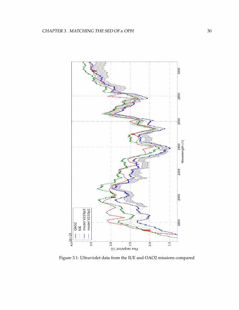
uncertainty. This perturbed data set was then convolved with the 50A boxcar filter. After
1000 Monte Carlo iterations, the mean and standard deviation of the resulting fluxes at
each sampled wavelength were computed. Figure 3.1 shows a comparison between the
OAO2 and the IUE observations. Although the two agree at some wavelengths within the
uncertainty, there are many wavelengths at which they do not. There will be models that
we can match to either one of the observed data sets. For this work we chose to compare
our synthetic SEDs with the IUE flux distribution given it’s high resolution which also al-
lowed comparison of fine details such as individual line profiles. Putting together the IUE
and visual data also carries some complications because they do not overlap in the UV and
there is no reference of which one provides better flux measurements in this region.
For this work, one suite composed of 4 different ROTORC models with different angu-
lar momentum distributions was selected as the best fit to the observed SED. All of them
were calculated to have the same observed shape and other basic parameters of α Oph (see
Table 1.1). The next subsection will give a description of how these models were calculated.
3.1 Rotating Models
During an attempt to match the p-mode oscillation modes, Deupree (2011) found a model
identified as “V240” which had the observed oblateness. However, a comparison of the
observed SED with the computed SED at the α Oph inclination showed that the model ef-
fective temperature was too high. New models were obtained by performing a few evolu-
tionary time steps (thus moving to cooler effective temperatures), which change the com-
CHAPTER 3. MATCHING THE SED OF α OPH 30
Figure 3.1: Ultraviolet data from the IUE and OAO2 missions compared
CHAPTER 3. MATCHING THE SED OF α OPH 31
position in the convective core and the surrounding area as the convective core shrinks.
During this “evolution” the shape is the only surface characteristic that is held constant.
The surface rotation velocities are no longer those required for an equipotential surface
to match the current (desired) surface shape, so the uniform rotation rate was scaled and
the model at the end of this evolution sequence re-converged, a process continued until
a uniform rotation rate was found which produced an equipotential surface that matched
the desired surface shape. Only a few evolutionary times steps were done at a time so that
the change in the surface equatorial velocity was only a few km s−1. The entire process
is repeated until there are a sufficiently large number of models with composition profiles
that look like those at various stages of an evolutionary sequence. Thus, these models
form a sequence of constant surface shape but decreasing effective temperature. It should
be noted, however, that these are not strictly speaking evolutionary sequences because we
have artificially constrained the rotation during the evolution in a way that does not con-
serve angular momentum. From the point of view of creating a 2D stellar model that can be
compared with data, not having obtained the model by a direct evolutionary sequence cal-
culation is irrelevant. We found a possible matching model (Deupree et al. 2012) denoted
V236 Xc25 that came from testing different parameters in the ROTORC model calculation.
This model not only matched the SED well (better than a spherical model would) but was
also able to match several high amplitude observed p-mode frequencies. Still, two issues
remained with V236 Xc25: one was the fact that the model didn’t come from an evolution-
ary path (it came from seemingly arbitrary changes of the stellar interior to get the right
shape and surface equatorial velocity) and the other the fact that the model represented
CHAPTER 3. MATCHING THE SED OF α OPH 32
a uniformly rotating star. All of ROTORC calculations mentioned above were performed
with the hydrogen mass fraction and the metals mass fraction of 0.7 and 0.02, respectively.
This abundance was used for all ROTORC calculations in this thesis, as well.
Having V236 Xc25 surface parameters as reference and still assuming uniform rotation
for simplicity, a new set of ROTORC calculations were performed by Dr. Deupree to obtain
a model that would be part of a evolution sequence and would also have the same shape,
surface temperatures and surface equatorial velocity. From this new set, the model V233p2
seemed like a perfect candidate matching most of V236 Xc25 surface values suggesting
that the calculated SED should have been very close between the two models, but instead
we found a some unexpected differences between them.
After careful examination we found that the difference came from non-uniform wave-
length vectors in the different PHOENIX model atmosphere files. This conflicts with the
CLIC execution, which expects an atmospheric grid with uniform values of wavelength
(same number of points and values) between all the intensity files. When V236 Xc25 was
calculated not all the PHOENIX intensity files had been cleansed of the added wavelengths
and later when the SED calculation of the V233p2 model was required, all the atmospheric
PHOENIX files had been interpolated in wavelength to have a ∆λ = 0.02. A recalcula-
tion of the SED produced by the V236 Xc25 model using the interpolated PHOENIX files
showed that it was very similar to the one of V233p2, as we initially expected.
Fixing this issue left the V236 Xc25 and V233p2 SEDs as a couple of models that didn’t
fit the IUE observations quite as well as before although still generally within the range
between the OAO2 and the IUE SED curves (see figure 3.1), so a new search for a uniformly
CHAPTER 3. MATCHING THE SED OF α OPH 33
rotating model was done. The work was not excessively complex given the fact that we
already knew which set of parameters we wanted to match and many models close to them
already existed.
After several iterations of SED comparisons, we found a uniformly rotating model, ID
V229p3, that best fit the observations. As evident from figure 3.1, which of the two models,
V233p2 or V229p3, fits the observations better depends on whether one gives more or less
weight to the OAO2 data in comparison to the IUE data. Clearly, more accurate ultravio-
let data would be invaluable in constraining the properties of the rotating models. From
V229p3 Dr. Deupree developed three other stellar models with slightly different internal
momentum distributions that still preserved the ratio of the polar to equatorial surface ra-
dius of α Oph. With this set we want to test if it is possible to determine whether the star
is differentially rotating just from the SED. Equation2.1 describes the differential rotation
law used to impose the internal rotation profile. Knowing that differential rotation changes
the shape of the star (thus changing the surface values), we looked for a range of values of
β that would produce a ROTORC model whose surface values still matched the observed
properties of α Oph within observational error. With a fixed to 2, the models that were
considered had values of β of 0.1, 0.2 and 0.4. The range of β was chosen to approximate
complete redistribution of angular momentum (uniform rotation) to local conservation of
angular momentum during stellar evolution except in the convective core. The properties
of the models selected are tabulated in Table 3.1. These models were chosen to keep the
surface equatorial radius nearly the same for possible comparison of oscillation frequen-
cies. Figure 3.2 presents a plot of the meridional plane to illustrate the difference in shape
CHAPTER 3. MATCHING THE SED OF α OPH 34
Figure 3.2: Cross section of the selected uniform rotating model (Blue curve) and the high-est differentially rotating model with β = 0.4 (Red curve).
between the uniform rotating model, V229p3, and the most differentially rotating model,
V209p95. Clearly, the changes in the surface structure are relatively modest.
3.2 Results
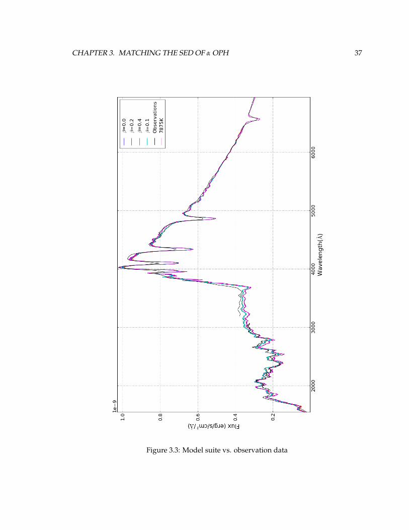
Figure 3.3 compares the SEDs of the four rotating models with the observations in the UV
and visible regions. Both the synthetic data and the measured data were filtered with a
boxcar filter of 50A of bandwidth and the distance of 14.6pc has been used to obtain the
CLIC fluxes.
All four models agree fairly well when compared with the observations, similar to the
CHAPTER 3. MATCHING THE SED OF α OPH 35
Table 3.1Properties of models considered
Model ID Veq Mass Luminosity Teq Req Rpole/Req Tpole/Teq β
(km s−1) (M�) (L�) (K) (R�)V229p3 229.3 2.1975 32.58 7570. 3.101 0.838 1.176 0V224 224. 2.20 32.60 7571. 3.101 0.838 1.179 0.1V219 219. 2.05 32.54 7569. 3.102 0.838 1.184 0.2V209p95 209.95 2.11 32.38 7569. 3.099 0.838 1.196 0.4
result we obtained for V236 Xc25 (Deupree et al. (2012)). From the figure it is clear that it
is difficult to detect sizeable differences between the uniform model and the others which
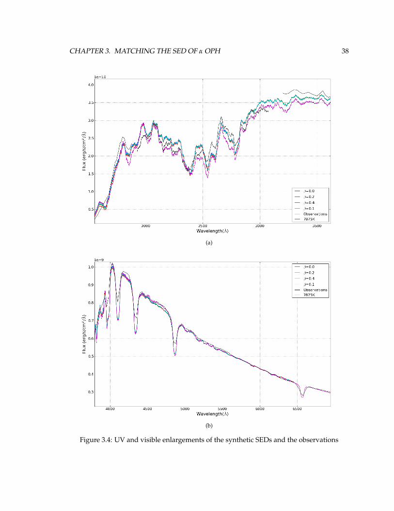
have different angular momentum distributions in their interior. Enlarged views of the UV
and the visible regions are shown on Figure 3.4a and 3.4b respectively. A quantitative test
was done to compare how well the rotational models fit the data compared to the spherical
model that best fit the observations (a non-rotating CLIC computed model with Te f f =
7875K). To quantify the comparison in the ultraviolet, we computed the the difference
between the observed flux and the computed fluxes every sampled point in the IUE dataset
from 1174A − 1878A and every 10A for the IUE dataset from 1900A − 3200A and then
calculated the standard deviation for these differences for each of the two IUE data sets.
The 10A sampling of the second IUE dataset produces more than a hundred points to
include in the calculation and is comparable to the sampling in the far UV dataset. To
make the comparison in the visual part of the spectrum the magnitude of the difference in
the fluxes was computed every 25A, which was the digitization frequency of the observed
data. The four rotating models are all close to each other, so for the sake of the comparison
with the spherical counterpart, only V229p3 was used.
CHAPTER 3. MATCHING THE SED OF α OPH 36
The fit to the data in the visible is about the same as that of the 7875 K effective temper-
ature model; they agree to within 1%. In the UV the standard deviation of the difference
between the observations and the rotating model was five times smaller compared to the
7875 K model for the far-ultraviolet data set (1174A− 1878A), although comparison of Fig-
ures 3.3 and 3.4 show that neither fits the SED perfectly. Each model is identified by its
β parameter, characterizing the amount of differential rotation included. We note that the
far-ultraviolet data set does not have the prominent peak at about 1600A that all rotating
models and the spherical model possess. This plays a role in the far-ultraviolet error com-
parison, making no model particularly good in the shortest wavelengths of this spectral
region. For the second IUE ultraviolet data set (1900A− 3200A), the rotating model SED
still fits better than the spherical model, having an average difference 35% smaller. Al-
though this better agreement with the observations for the rotating model SED provides
some validation both for the rotating models themselves and of the numerical approach of
integrating the localized surface temperatures and gravities over the surface to obtain the
observed flux, the uncertainty associated with these IUE observations hinders the possibil-
ity to pick one model as best-fit.
Figure 3.4a does show some differences among the SEDs for the different rotating mod-
els, but they are so small that hardly any conclusion can be drawn about the actual internal
angular momentum distribution of α Oph from just the SED, at least from the range chosen.
In light of the small differences between the rotating models and even the spherical
case considered, something that one might ask is how much does every latitudinal zone
contribute to the flux at each wavelength and how does it change with the inclination at
CHAPTER 3. MATCHING THE SED OF α OPH 37
Figure 3.3: Model suite vs. observation data
CHAPTER 3. MATCHING THE SED OF α OPH 38
(a)
(b)
Figure 3.4: UV and visible enlargements of the synthetic SEDs and the observations
CHAPTER 3. MATCHING THE SED OF α OPH 39
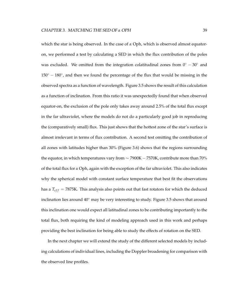
which the star is being observed. In the case of α Oph, which is observed almost equator-
on, we performed a test by calculating a SED in which the flux contribution of the poles
was excluded. We omitted from the integration colatitudinal zones from 0◦ − 30◦ and
150◦ − 180◦, and then we found the percentage of the flux that would be missing in the
observed spectra as a function of wavelength. Figure 3.5 shows the result of this calculation
as a function of inclination. From this ratio it was unexpectedly found that when observed
equator-on, the exclusion of the pole only takes away around 2.5% of the total flux except
in the far ultraviolet, where the models do not do a particularly good job in reproducing
the (comparatively small) flux. This just shows that the hottest zone of the star’s surface is
almost irrelevant in terms of flux contribution. A second test omitting the contribution of
all zones with latitudes higher than 30% (Figure 3.6) shows that the regions surrounding
the equator, in which temperatures vary from∼ 7900K− 7570K, contribute more than 70%
of the total flux for α Oph, again with the exception of the far ultraviolet. This also indicates
why the spherical model with constant surface temperature that best fit the observations
has a Te f f = 7875K. This analysis also points out that fast rotators for which the deduced
inclination lies around 40◦ may be very interesting to study. Figure 3.5 shows that around
this inclination one would expect all latitudinal zones to be contributing importantly to the
total flux, both requiring the kind of modeling approach used in this work and perhaps
providing the best inclination for being able to study the effects of rotation on the SED.
In the next chapter we will extend the study of the different selected models by includ-
ing calculations of individual lines, including the Doppler broadening for comparison with
the observed line profiles.
CHAPTER 3. MATCHING THE SED OF α OPH 40
Figure 3.5: Percentage of flux lost from the V229p3 model when the polar region is ex-cluded from the calculation. We set the polar region to be between 0◦− 30◦, and 150◦− 180◦
in latitude.
CHAPTER 3. MATCHING THE SED OF α OPH 41
Figure 3.6: Percentage of flux subtracted from the V229p3 model when a region of 60◦ fromthe pole is excluded from the CLIC integration.
Chapter 4
Lines
It was effectively impossible to determine which rotation law fits what we observe from α
Oph better by comparing only the full SED because the difference were so small. However,
it is conceivable that studying individual spectral lines could provide a better discriminant
of the rotation law. We thus used the same set of models as in the SED analysis to look at
differences in several line profiles between these models and the observations of α Oph.
Potentially, these comparison plots could identify a model with a certain internal angular
momentum distribution as the best fit.
CLIC has the ability to synthesize individual spectral lines including all rotational ef-
fects. There is no need to invoke any limb or gravity darkening law because the atmo-
spheric and internal model construction of the star provide the necessary data to calculate
the real effect in the line profile. Unlike SED calculations, in “line mode” CLIC includes
the Doppler effect of rotation as well. We began by searching for prominent lines in the
observed ultraviolet and visual spectra of α Oph. Once a line was selected, PHOENIX
42
CHAPTER 4. LINES 43
provided the identification of every absorption feature, including the element name and
ionization stage. With all this information however, the identification of lines (particularly
in the UV part of the spectra) became a challenge. As expected, iron dominated most of
the SED absorption features between 1500 and 3000A, with most lines being blended. Five
lines were selected in this wavelength range by visual inspection for comparison with the
IUE observations. The selection was based on their absorption strength and how many
elements were responsible for each one of them. We wanted to study lines that were pro-
duced only by one element, hence containing only the Doppler broadening in their profile,
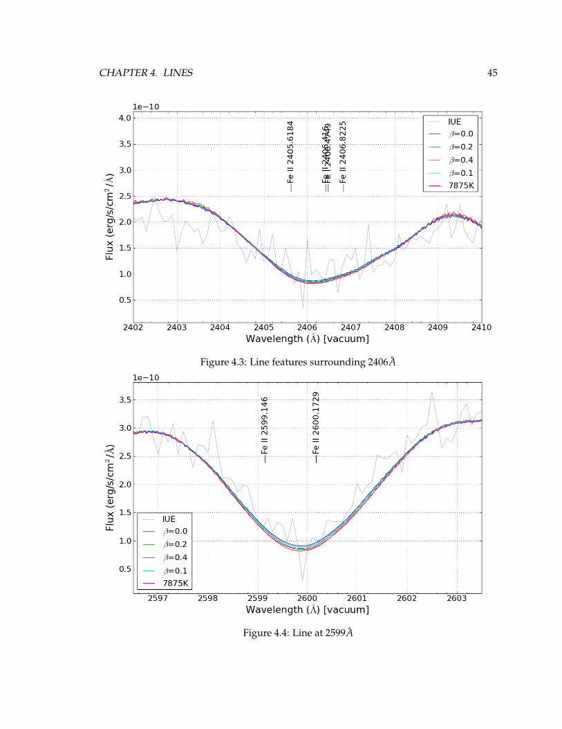
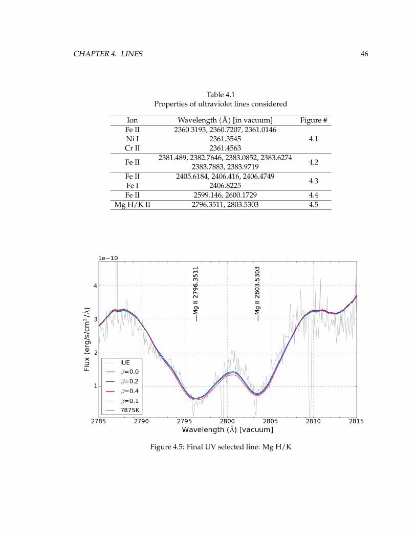
but this proved to be almost impossible with the exception of three cases in the UV, a FeII
line at 2599A and the Mg H/K lines at 2799A and 2801A. The rest of the line features
selected have various elements as responsible members of the absorption. A summarized
list with all the spectral lines considered is given in Table 4.1 and the corresponding com-
parison plots are shown in Figures 4.1 to 4.5. As in the study of the SED, we included the
observed spectrum and the spectra computed for the models in Table 3.1. We have also cal-
culated with CLIC the line profiles of the best fit spherical model of Te f f = 7875K assuming
the rotational velocities of the uniform rotating model to include the Doppler broadening
effect. This was the only rotational effect included in the spherical model.
From the complete SED analysis we know that the continuum for our models does not
perfectly match the averaged IUE continuum, but here what we wish to focus on is how the
different angular momentum distributions would affect the line profiles themselves and
how they will compare with the observations. With this in mind, for each line we matched
the continuum surrounding the line by multiplying the computed flux by a constant. This
CHAPTER 4. LINES 44
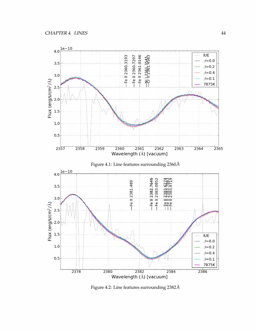
Figure 4.1: Line features surrounding 2360A
Figure 4.2: Line features surrounding 2382A
CHAPTER 4. LINES 45
Figure 4.3: Line features surrounding 2406A
Figure 4.4: Line at 2599A
CHAPTER 4. LINES 46
Table 4.1Properties of ultraviolet lines considered
Ion Wavelength (A) [in vacuum] Figure #Fe II 2360.3193, 2360.7207, 2361.0146
4.1Ni I 2361.3545Cr II 2361.4563
Fe II2381.489, 2382.7646, 2383.0852, 2383.6274
4.22383.7883, 2383.9719
Fe II 2405.6184, 2406.416, 2406.47494.3
Fe I 2406.8225Fe II 2599.146, 2600.1729 4.4
Mg H/K II 2796.3511, 2803.5303 4.5
Figure 4.5: Final UV selected line: Mg H/K
CHAPTER 4. LINES 47
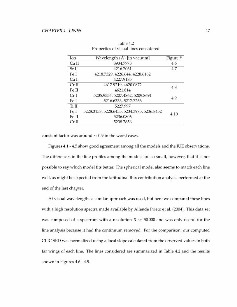
Table 4.2Properties of visual lines considered
Ion Wavelength (A) [in vacuum] Figure #Ca II 3934.7773 4.6Sr II 4216.7061 4.7Fe I 4218.7329, 4226.644, 4228.6162Ca I 4227.9185Cr II 4617.9219, 4620.0872
4.8Fe II 4621.814Cr I 5205.9556, 5207.4862, 5209.8691
4.9Fe I 5216.6333, 5217.7266Ti II 5227.997
4.10Fe I 5228.3158, 5228.6455, 5234.3975, 5236.8452Fe II 5236.0806Cr II 5238.7856
constant factor was around ∼ 0.9 in the worst cases.
Figures 4.1 - 4.5 show good agreement among all the models and the IUE observations.
The differences in the line profiles among the models are so small, however, that it is not
possible to say which model fits better. The spherical model also seems to match each line
well, as might be expected from the latitudinal flux contribution analysis performed at the
end of the last chapter.
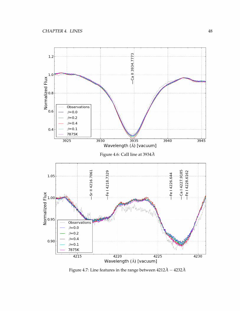
At visual wavelengths a similar approach was used, but here we compared these lines
with a high resolution spectra made available by Allende Prieto et al. (2004). This data set
was composed of a spectrum with a resolution R ' 50 000 and was only useful for the
line analysis because it had the continuum removed. For the comparison, our computed
CLIC SED was normalized using a local slope calculated from the observed values in both
far wings of each line. The lines considered are summarized in Table 4.2 and the results
shown in Figures 4.6 - 4.9.
CHAPTER 4. LINES 48
Figure 4.6: CaII line at 3934A
Figure 4.7: Line features in the range between 4212A− 4232A
CHAPTER 4. LINES 49
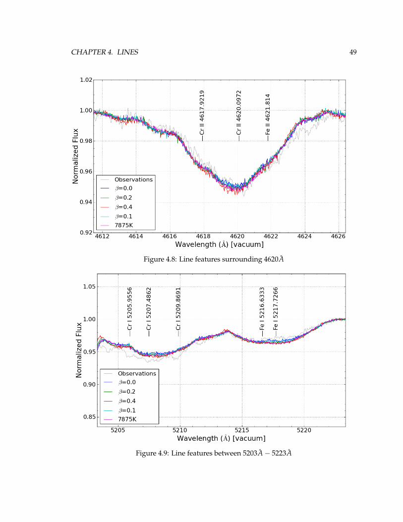
Figure 4.8: Line features surrounding 4620A
Figure 4.9: Line features between 5203A− 5223A
CHAPTER 4. LINES 50
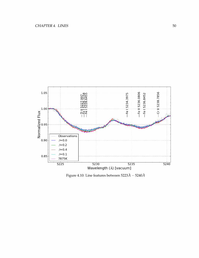
Figure 4.10: Line features between 5223A− 5240A
CHAPTER 4. LINES 51
The plots show that the agreement between line profiles in the models and the observa-
tions continues in the visible. Small differences can be seen in some cases (e.g. Figure 4.9).
For this particular case it is unlikely that that problem is in the iron abundance because we
match other iron lines rather well (e.g. Figure 4.4).
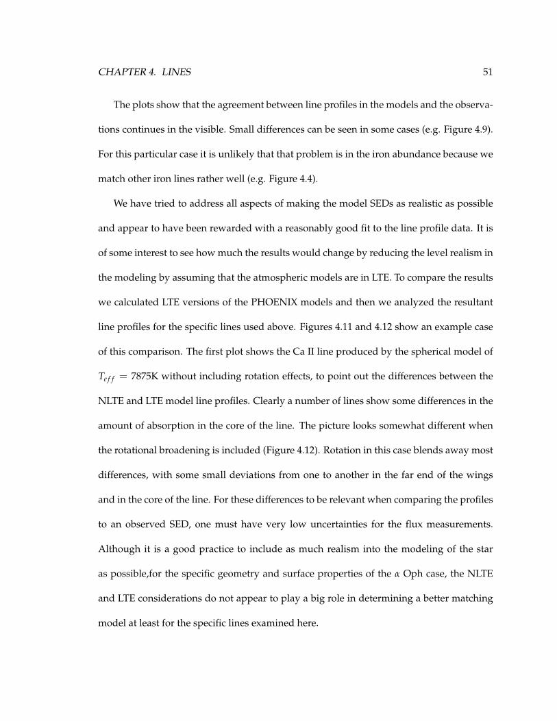
We have tried to address all aspects of making the model SEDs as realistic as possible
and appear to have been rewarded with a reasonably good fit to the line profile data. It is
of some interest to see how much the results would change by reducing the level realism in
the modeling by assuming that the atmospheric models are in LTE. To compare the results
we calculated LTE versions of the PHOENIX models and then we analyzed the resultant
line profiles for the specific lines used above. Figures 4.11 and 4.12 show an example case
of this comparison. The first plot shows the Ca II line produced by the spherical model of
Te f f = 7875K without including rotation effects, to point out the differences between the
NLTE and LTE model line profiles. Clearly a number of lines show some differences in the
amount of absorption in the core of the line. The picture looks somewhat different when
the rotational broadening is included (Figure 4.12). Rotation in this case blends away most
differences, with some small deviations from one to another in the far end of the wings
and in the core of the line. For these differences to be relevant when comparing the profiles
to an observed SED, one must have very low uncertainties for the flux measurements.
Although it is a good practice to include as much realism into the modeling of the star
as possible,for the specific geometry and surface properties of the α Oph case, the NLTE
and LTE considerations do not appear to play a big role in determining a better matching
model at least for the specific lines examined here.
CHAPTER 4. LINES 52
Figure 4.11: Line profile comparison between the best-fit spherical atmospheric model inNLTE and the model in LTE. The lines have not been rotationally broadened.
CHAPTER 4. LINES 53
Figure 4.12: Broadened line profile comparison between the best-fit spherical atmosphericmodel in NLTE and the nodel in LTE
Chapter 5
Conclusions
The goal of this work was to compare the SEDs and absorption line profiles of theoretical
stellar models that included slightly different internal angular momentum distributions
with the observed SED and line profiles of the rapidly rotating, δ Scuti star, α Oph. This
star is an interesting case for study because many of its surface properties (inclination,
oblateness, temperature difference between pole and equator) have been deduced through
interferometry, so the degrees of freedom in the stellar model generation are greatly re-
duced. The asteroseismic observations make α Oph a good test probe of detailed models
of rotating stars.
We have already presented a first attempt of matching the SED with a uniformly rotat-
ing model (Deupree et al. 2012), achieving a good fit to observations. This fit was also better
than that of a spherical model with the deduced effective temperature of the star. However,
one would expect for a star as evolved as α Oph (expected to be in relatively late core hy-
drogen burning) that uniform rotation is not the most likely rotation law. While there is no
54
CHAPTER 5. CONCLUSIONS 55
reason to believe that the rotation law remains conservative because the stellar core proba-
bly rotates somewhat more rapidly than the outer layers, we have approximated plausible
rotation rates by three conservative differentially rotating models in which the material
closer to the polar axis rotates more rapidly than the material farther away. All models
matched the interferometric oblateness, although the surface shapes at mid latitudes were
slightly different. The non-LTE stellar atmosphere and spectrum synthesis code PHOENIX
was used to generate a grid of plane-parallel stellar atmospheres which covered the full
range of effective temperature and effective gravity values at all latitudes for all the mod-
els of α Oph. Finally, the intensity integrator code CLIC was used to calculate SEDs and
absorption line profiles from the ROTORC models for comparison with available observa-
tions of α Oph. One of the advantages of the procedure followed here is that there is no
need to include any limb or gravity darkening law into account because the atmospheric
and internal model construction of the star provide the necessary data to calculate the real
effect on the SED and line profile.
We selected a well-exposed pair of IUE spectra and also an OAO2 dataset that covered
the ultraviolet spectrum from 1150A to 3200A. The IUE had good resolution but a fairly
high standard deviation for each flux measurement, while the OAO2 had a small standard
deviation but a relatively low resolution. After filtering the IUE data with a 50A wide
boxcar filter, both agree within uncertainties in some, but not all, wavelength regions, but
it is not possible to select one as better than the other without having more observations.
We chose to compare our results with the higher resolved IUE data set to be able to compare
the line profiles. We were able to fit the observed SEDs fairly well with our model SEDs in
CHAPTER 5. CONCLUSIONS 56
both the UV and the visual, and the line profile fits to the data were generally quite good.
The SED comparison showed that the four selected ROTORC models with different
internal angular momentum distributions produce SEDs which are very close to each other,
and it is very hard to distinguish any one model from the others. Each of the four models
provide a reasonable fit to the observed SEDs in both the ultraviolet and visual parts of the
spectrum. They also show that for a star that is differentially rotating following equation
2.1 with values of β = 0.1− 0.4, it is almost impossible to say which model resembles more
closely the real internal rotational profile of α Oph. We also found that by observing the star
equator-on, most of the flux contribution comes from latitudes around the equator even
though the equatorial region is noticeably cooler than the higher latitudes. An exclusion of
a 30◦ latitude zone around the pole removes only∼ 2.5% of the total flux for all wavelength
regions studied except those in the far ultraviolet where the total flux is comparatively
small. This analysis shows that a very interesting case to study would be a rapidly rotating
star observed to be inclined at around 40◦, a configuration in which the visible surface of
both the pole and the equator would play an important role in the observed SED.
We extended the analysis of the same set of models by considering individual line pro-
files. The selection of each line was done by visual inspection of both the synthetic SEDs
and the observations. We looked for prominent features that if possible were composed
of just one element. The PHOENIX code provided the identification of each line. Vertical
scaling was required in some of the models because the observed and modeled continua
were not always perfectly matched, as was seen in the SED comparison for all the models
with respect to the observations. The scaling factor departed from unity by about 10% in
CHAPTER 5. CONCLUSIONS 57
the worst cases. After the continuum was adjusted, the lines calculated with CLIC agreed
well with the observational data and, once again, the differences between each model in
the suite were too small to definitely point to a single model as the one which provided the
best fit.
It is thus difficult to determine a best-fit β parameter just from the calculated SED and
individual lines for these low differential rotation regimes. One last test for this suite of
models, beyond the scope of this work, would be to consider their oscillation properties
and how well they compare with the MOST data for α Oph. This might shed light on a
preferred model that describes better the possible internal configuration on the star.
A interesting future case of study would be the historically important photometric
standard star, Vega, which was discovered to be rapidly rotating from the anomalous flat-
bottomed appearance of many of its weak metal lines, which could only be explained by
model of a star seen nearly pole-on (i ∼ 5◦) and rotating at around 245 km/s at the equator
(Gulliver et al. 1991, 1994). More recently, Aufdenberg et al. (2006) studied Vega interfer-
ometrically with the CHARA array and found values of i = 4.7◦ ± 0.3◦ and an equatorial
velocity of (270± 15)km/s by fitting rotating models that included gravity darkening ap-
proximations. We could potentially provide a better constraint on the properties of Vega
by applying the method followed in this work for α Oph, with the advantage that in Vega’s
case the amount of observational data available is quite large and of better quality. Thought
to have an inclination of ∼ 57◦, Altair presents another interesting case (Monnier et al.
2007). For this inclination, both the polar and equatorial regions would be expected to con-
tribute significantly to the flux. Such a case might provide a better test of both the rotating
CHAPTER 5. CONCLUSIONS 58
models and the approach used. van Belle (2012) presents a catalog of 354 new possible
rapid rotating targets that can be resolved interferometrically with current instrumenta-
tion, suggesting that there will be many opportunities to apply our method and maybe
help understand the physics of the interior of rotating stars.

Bibliography
Abt, H. A., Levato, H., & Grosso, M. 2002, The Astrophysical Journal, 573, 359
Abt, H. A. & Morrell, N. I. 1995, The Astrophysical Journal Supplement Series, 99, 135
Allen, C. W. 1973, Astrophysical Quantities, 3rd edn.
Allende Prieto, C., Barklem, P. S., Lambert, D. L., & Cunha, K. 2004, Astronomy and Astro-
physics, 420, 183
Aufdenberg, J. P., Merand, A., du Foresto, V. C., et al. 2006, The Astrophysical Journal, 645,
664
Bautista, M. A., Romano, P., & Pradhan, A. K. 1998, The Astrophysical Journal Supplement
Series, 118, 259
Bernacca, P. L. & Perinotto, M. 1970, Contr. Oss. Astrof. Padova in Asiago
Blackwell, D. E. & Lynas-Gray, A. E. 1998, Astronomy and Astrophysics Supplement Series,
129, 505
Bodenheimer, P. 1971, The Astrophysical Journal, 167, 153
59
BIBLIOGRAPHY 60
Breger, M. 2000, Delta Scuti and Related Stars, 210
Burnashev, V. 1985, Abastumanskaya Astrofiz. Obs. Bull., 59
Carciofi, A. C., Domiciano de Souza, A., Magalhaes, A. M., Bjorkman, J. E., & Vakili, F.
2008, The Astrophysical Journal, 676, L41
Carroll, J. A. 1928, Monthly Notices of the Royal Astronomical Society, 88, 548
Carroll, J. A. 1933, Monthly Notices of the Royal Astronomical Society, 93, 478
Che, X., Monnier, J. D., Zhao, M., et al. 2011, The Astrophysical Journal, 732, 68
Claret, A. 2003, Astronomy and Astrophysics, 406, 623
Clement, M. J. 1974, The Astrophysical Journal, 194, 709
Clement, M. J. 1978, The Astrophysical Journal, 222, 967
Clement, M. J. 1979, The Astrophysical Journal, 230, 230
Code, A. D. & Meade, M. R. 1979, The Astrophysical Journal Supplement Series, 39, 195
Collins, G. W. 1963, The Astrophysical Journal, 138, 1134
Collins, G. W. & Truax, R. J. 1995, The Astrophysical Journal, 439, 860
Collins, G. W., Truax, R. J., & Cranmer, S. R. 1991, The Astrophysical Journal Supplement
Series, 77, 541
Crawford, I. 2001, Monthly Notices of the Royal Astronomical Society, 327, 841
BIBLIOGRAPHY 61
Demarque, P., Guenther, D. B., Li, L. H., Mazumdar, A., & Straka, C. W. 2007, Astrophysics
and Space Science, 316, 31
Deupree, R. G. 1990, The Astrophysical Journal, 357, 175
Deupree, R. G. 1995, The Astrophysical Journal, 439, 357
Deupree, R. G. 1998, The Astrophysical Journal, 499, 340
Deupree, R. G. 2011, The Astrophysical Journal, 742, 9
Deupree, R. G., Castaneda, D., Pena, F., & Short, C. I. 2012, The Astrophysical Journal, 753,
20
Domiciano de Souza, A., Kervella, P., Jankov, S., et al. 2003, Astronomy and Astrophysics,
407, L47
Drawin, H. W. 1961, Zeitschrift fur Physik, 164, 513
Eggenberger, P., Meynet, G., Maeder, A., et al. 2007, Astrophysics and Space Science, 316,
43
Endal, A. S. & Sofia, S. 1976, The Astrophysical Journal, 210, 184
Endal, A. S. & Sofia, S. 1978, The Astrophysical Journal, 220, 279
Erspamer, D. & North, P. 2003, Astronomy and Astrophysics, 398, 1121
Espinosa Lara, F. 2010, Astrophysics and Space Science, 328, 291
Faulkner, J., Roxburgh, I. W., & Strittmatter, P. A. 1968, The Astrophysical Journal, 151, 203
BIBLIOGRAPHY 62
Fremat, Y., Zorec, J., Hubert, A.-M., & Floquet, M. 2005, Astronomy and Astrophysics, 440,
305
Gatewood, G. 2005, The Astronomical Journal, 130, 809
Gillich, A. 2007, Master’s Thesis, Saint Mary’s University, Halifax, Nova Scotia
Gillich, A., Deupree, R. G., Lovekin, C. C., Short, C. I., & Toque, N. 2008, The Astrophysical
Journal, 683, 441
Gray, R. O., Graham, P. W., & Hoyt, S. R. 2001, The Astronomical Journal, 121, 2159
Gulliver, A. F., Adelman, S. J., Cowley, C. R., & Fletcher, J. M. 1991, The Astrophysical
Journal, 380, 223
Gulliver, A. F., Hill, G., & Adelman, S. J. 1994, The Astrophysical Journal, 429, L81
Hauschildt, P. H. & Baron, E. 1999, J. Comput. Appl. Math., 109
Hinkley, S., Monnier, J. D., Oppenheimer, B. R., et al. 2011, The Astrophysical Journal, 726,
104
Jackson, S. 1970, The Astrophysical Journal, 161, 579
Jackson, S., MacGregor, K. B., & Skumanich, A. 2004, The Astrophysical Journal, 606, 1196
Jackson, S., MacGregor, K. B., & Skumanich, A. 2005, The Astrophysical Journal Supple-
ment Series, 156, 245
Johnson, H. L. & Harris, D. L. 1954, The Astrophysical Journal, 120, 196
BIBLIOGRAPHY 63
Johnson, H. L. & Knuckles, C. F. 1957, The Astrophysical Journal, 126, 113
Johnson, H. L., Mitchell, R. I., Iriarte, B., & Wisniewski, W. Z. 1966, Communications of the
Lunar and Planetary Laboratory, 4
Kanaan, S., Meilland, A., Stee, P., et al. 2008, Astronomy and Astrophysics, 486, 785
Kervella, P., Domiciano de Souza, A., Kanaan, S., et al. 2009, Astronomy and Astrophysics,
493, L53
Kippenhahn, R. 1977, Astronomy and Astrophysics, 58, 267
Kippenhahn, R., Meyer-Hofmeister, E., & Thomas, H. C. 1970, Astronomy and Astro-
physics, 5
Kippenhahn, R. & Thomas, H. 1970, Stellar Rotation
Kurucz, R. 1994, Atomic Data for Fe and Ni (Cambridge: SAO)
Kurucz, R. L. & Bell, B. 1995, Atomic Line List (Cambridge: SAO)
Linnell, A. P. & Hubeny, I. 1994, The Astrophysical Journal, 434, 738
Lovekin, C. 2005, Master’s Thesis, Saint Mary’s University, Halifax, Nova Scotia
Lovekin, C. C., Deupree, R. G., & Short, C. I. 2006, The Astrophysical Journal, 643, 460
Lucy, L. B. 1967, Zeitschrift fur Astrophysik, 65
MacGregor, K. B., Jackson, S., Skumanich, A., & Metcalfe, T. S. 2007, The Astrophysical
Journal, 663, 560
BIBLIOGRAPHY 64
Maeder, A. 1999, Astronomy and Astrophysics, 347, 185
Maeder, A. & Peytremann, E. 1970, Astronomy and Astrophysics, 7, 120
Malagnini, M. L. & Morossi, C. 1990, Astronomy and Astrophysics Supplement Series
(ISSN 0365-0138), 85, 1015
Mathisen, R. 1984, Photo Cross Sections for Stellar Atmosphere Calculations: Compilation
of References and Data (Oslo: Univ. Oslo)
McAlister, H. A., ten Brummelaar, T. A., Gies, D. R., et al. 2005, The Astrophysical Journal,
628, 439
Monaghan, F. F. & Roxburgh, I. W. 1965, Monthly Notices of the Royal Astronomical Soci-
ety, 131
Monnier, J. D., Townsend, R. H. D., Che, X., et al. 2010, The Astrophysical Journal, 725,
1192
Monnier, J. D., Zhao, M., Pedretti, E., et al. 2007, Science (New York, N.Y.), 317, 342
Ostriker, J. P. & Mark, J. W.-K. 1968, The Astrophysical Journal, 151, 1075
Paturel, G., Petit, C., Prugniel, P., et al. 2003, Astronomy and Astrophysics, 412, 45
Reilman, R. F. & Manson, S. T. 1979, The Astrophysical Journal Supplement Series, 40, 815
Reiners, A. 2003, Astronomy and Astrophysics, 408, 707
Roxburgh, I. W., Griffith, J. S., & Sweet, P. A. 1965, Zeitschrift fur Astrophysik, 61
BIBLIOGRAPHY 65
Royer, F., Grenier, S., Baylac, M.-O., Gı¿œmez, A. E., & Zorec, J. 2002, Astronomy and
Astrophysics, 393, 897
Sackmann, I.-J. & Anand, S. P. S. 1970, The Astrophysical Journal, 162, 105
Seaton, M. J., Yan, Y., Mihalas, D., & Pradhan, A. K. 1994, Monthly Notices of the Royal
Astronomical Society, 266
Shajn, G. & Struve, O. 1929, Monthly Notices of the Royal Astronomical Society, 89, 222
Short, C. I., Hauschildt, P. H., & Baron, E. 1999, The Astrophysical Journal, 525, 375
Slettebak, A. 1949, The Astrophysical Journal, 110, 498
Slettebak, A., Kuzma, T. J., & Collins, G. W. 1980, The Astrophysical Journal, 242, 171
Townsend, R. H. D., Owocki, S. P., & Howarth, I. D. 2004, Monthly Notices of the Royal
Astronomical Society, 350, 189
Uesuga, A. & Fukuda, I. 1970, MnKyo, 33, 205
van Belle, G. T. 2012, The Astronomy and Astrophysics Review, 20, 51
van Belle, G. T., Ciardi, D. R., Thompson, R. R., Akeson, R. L., & Lada, E. A. 2001, The
Astrophysical Journal, 559, 1155
Vinicius, M. M. F., Zorec, J., Leister, N. V., & Levenhagen, R. S. 2006, Astronomy and Astro-
physics, 446, 643
von Zeipel, H. 1924, Monthly Notices of the Royal Astronomical Society, 84, 665

BIBLIOGRAPHY 66
Xu, Y., Li, Z.-P., Deng, L.-C., & Xiong, D.-R. 2002, Chinese Journal of Astronomy &
Astrophysics, 2, 441
Zhao, M., Monnier, J. D., Pedretti, E., et al. 2009, The Astrophysical Journal, 701, 209