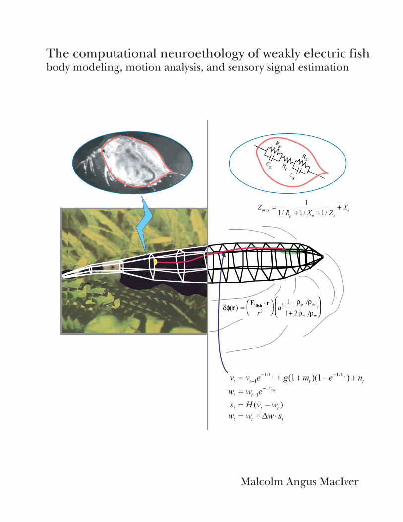
δφ(r) =Efish ⋅r

r3

a3

1− ρp /ρw

1+ 2ρp /ρw

Rs

RsCs

Cs

Ri

ttt wvHs −= )(tt eww w= −−

/11

t

tttt nemgevv vv +−++= −−− )1)(1( /1/1

1tt

ttt swww ⋅∆+=

The computational neuroethology of weakly electric fishbody modeling, motion analysis, and sensory signal estimation

Malcolm Angus MacIver

Zprey = 11/ Rp +1/ Xp +1/ Zs

+ Xs

µV Spikes/s

A B

Time

t = 333 ms

t = 167 ms

t = 0 ms

t = -167 ms

Detection

Transdermal Potential Change Afferent Firing Rate Change

8

10

6

4

2

0

5

10

0

-5

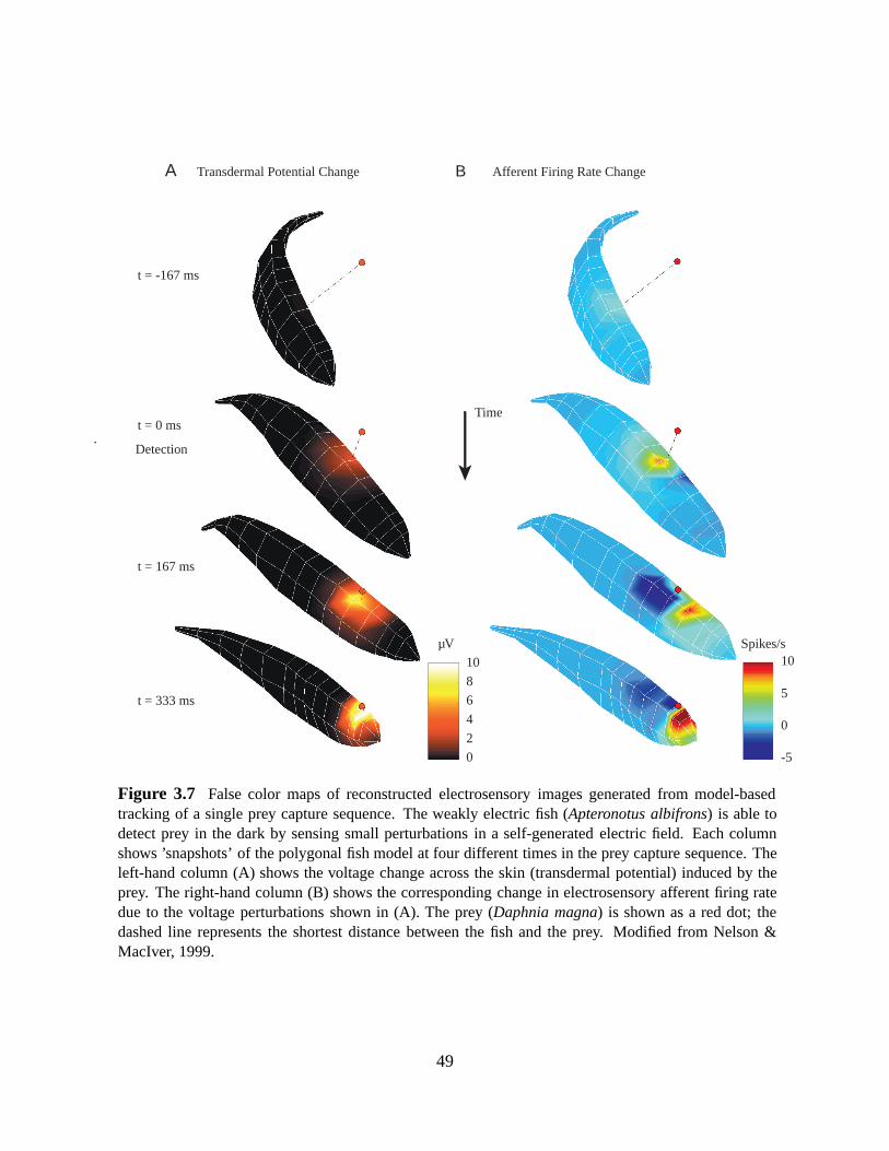
Figure 3.7 False color maps of reconstructed electrosensory images generated from model-basedtracking of a single prey capture sequence. The weakly electricfish (Apteronotus albifrons) is able todetect prey in the dark by sensing small perturbations in a self-generated electricfield. Each columnshows’snapshots’ of the polygonalfish model at four different times in the prey capture sequence. Theleft-hand column (A) shows the voltage change across the skin (transdermal potential) induced by theprey. The right-hand column (B) shows the corresponding change in electrosensory afferentfiring ratedue to the voltage perturbations shown in (A). The prey (Daphnia magna) is shown as a red dot; thedashed line represents the shortest distance between thefish and the prey. Modified from Nelson &MacIver, 1999.

49

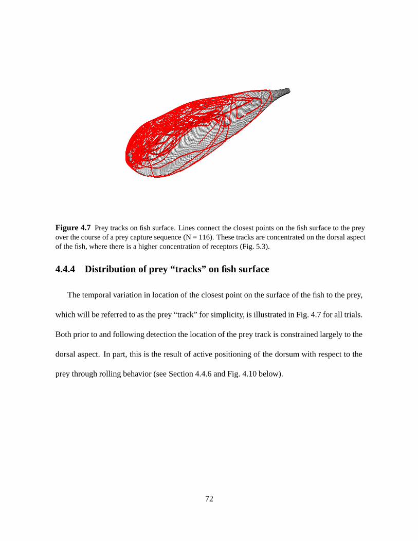
Figure 4.7 Prey tracks onfish surface. Lines connect the closest points on thefish surface to the preyover the course of a prey capture sequence (N = 116). These tracks are concentrated on the dorsal aspectof thefish, where there is a higher concentration of receptors (Fig. 5.3).

4.4.4 Distribution of prey “tracks” on fish surface

The temporal variation in location of the closest point on the surface of thefish to the prey,

which will be referred to as the prey“track” for simplicity, is illustrated in Fig. 4.7 for all trials.

Both prior to and following detection the location of the prey track is constrained largely to the

dorsal aspect. In part, this is the result of active positioning of the dorsum with respect to the

prey through rolling behavior (see Section 4.4.6 and Fig. 4.10 below).

72

0

1

2

3

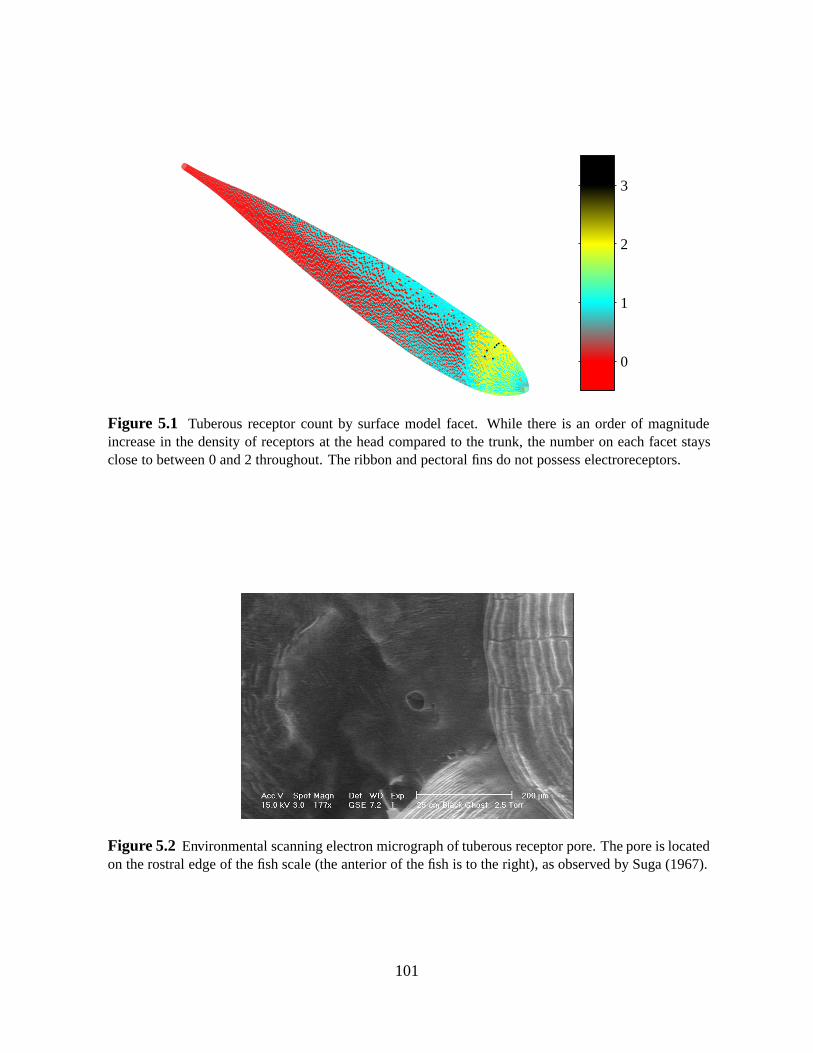
Figure 5.1 Tuberous receptor count by surface model facet. While there is an order of magnitudeincrease in the density of receptors at the head compared to the trunk, the number on each facet staysclose to between 0 and 2 throughout. The ribbon and pectoralfins do not possess electroreceptors.

Figure 5.2 Environmental scanning electron micrograph of tuberous receptor pore. The pore is locatedon the rostral edge of thefish scale (the anterior of thefish is to the right), as observed by Suga (1967).

101

15

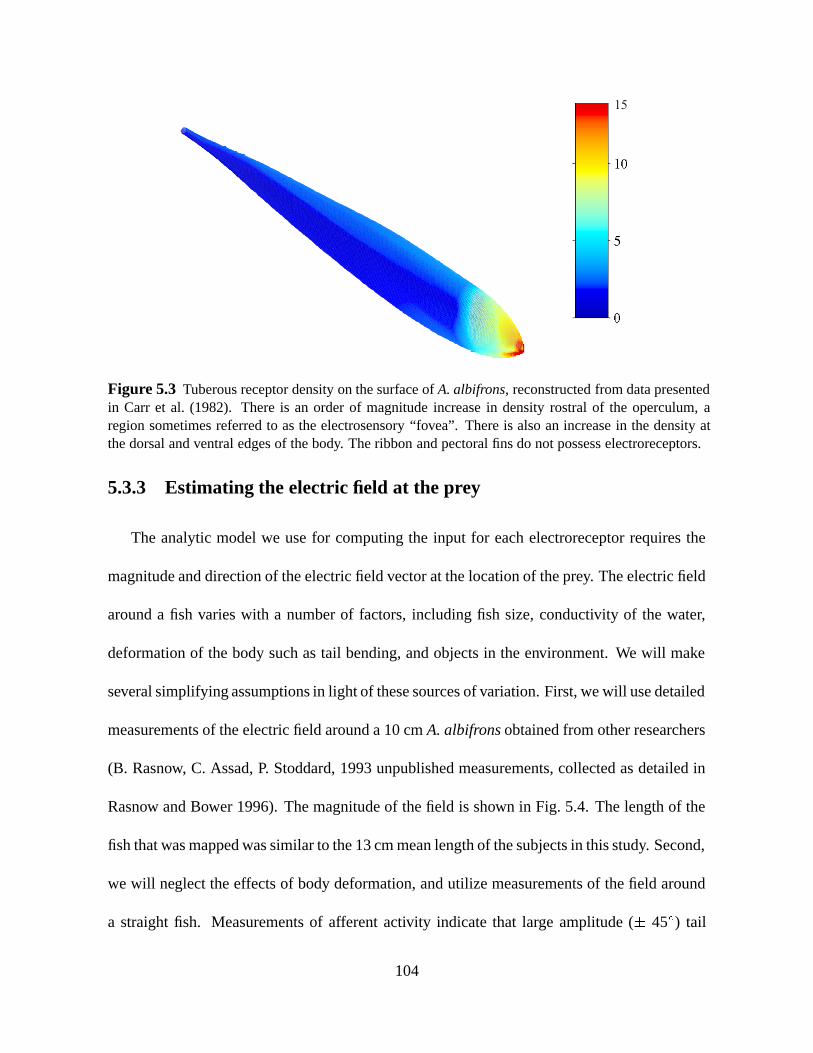
Figure 5.3 Tuberous receptor density on the surface ofA. albifrons, reconstructed from data presentedin Carr et al. (1982). There is an order of magnitude increase in density rostral of the operculum, aregion sometimes referred to as the electrosensory “fovea”. There is also an increase in the density atthe dorsal and ventral edges of the body. The ribbon and pectoral fins do not possess electroreceptors.

5.3.3 Estimating the electric field at the prey

The analytic model we use for computing the input for each electroreceptor requires the

magnitude and direction of the electric field vector at the location of the prey. The electric field

around a fish varies with a number of factors, including fish size, conductivity of the water,

deformation of the body such as tail bending, and objects in the environment. We will make

several simplifying assumptions in light of these sources of variation. First, we will use detailed

measurements of the electric field around a 10 cmA. albifrons obtained from other researchers

(B. Rasnow, C. Assad, P. Stoddard, 1993 unpublished measurements, collected as detailed in

Rasnow and Bower 1996). The magnitude of the field is shown in Fig. 5.4. The length of the

fish that was mapped was similar to the 13 cm mean length of the subjects in this study. Second,

we will neglect the effects of body deformation, and utilize measurements of the field around

a straight fish. Measurements of afferent activity indicate that large amplitude ( 45Æ) tail

104

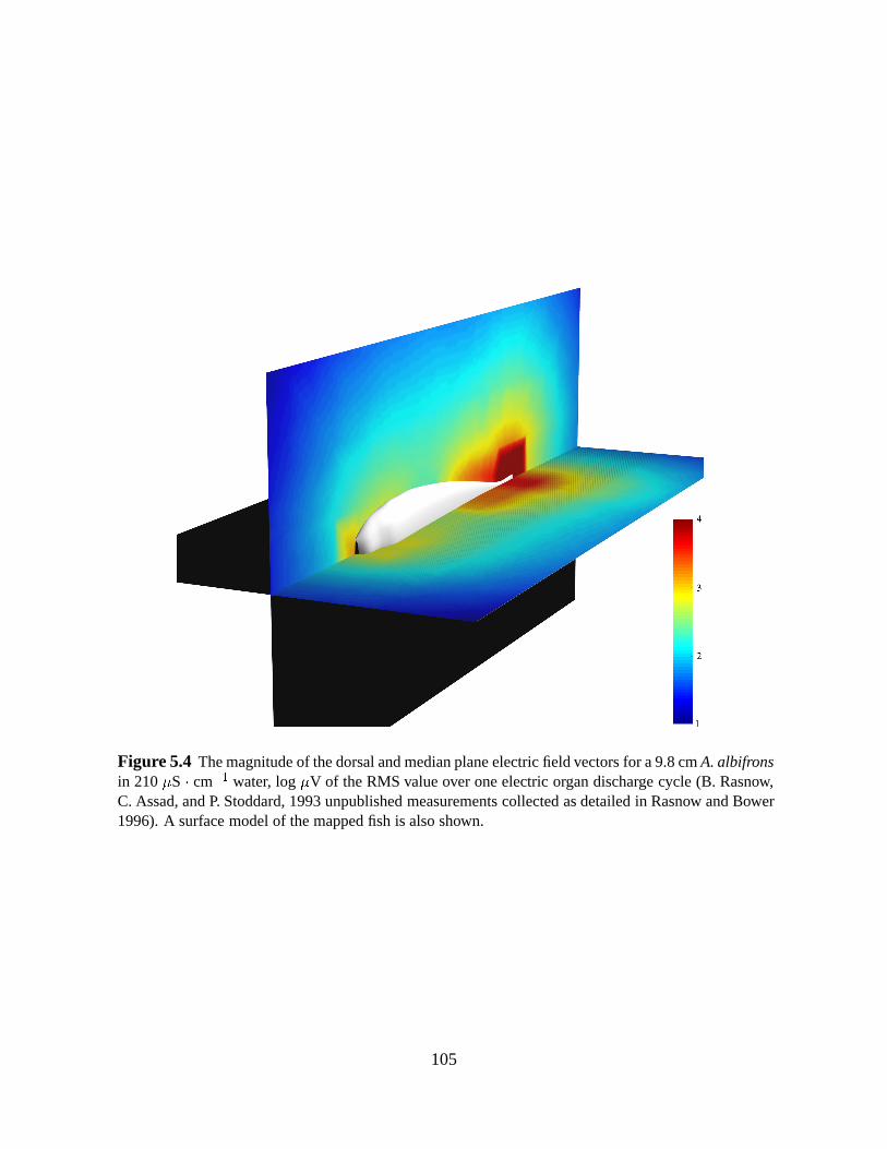
Figure 5.4 The magnitude of the dorsal and median plane electricfield vectors for a 9.8 cmA. albifronsin 210S cm1 water, logV of the RMS value over one electric organ discharge cycle (B. Rasnow,C. Assad, and P. Stoddard, 1993 unpublished measurements collected as detailed in Rasnow and Bower1996). A surface model of the mappedfish is also shown.

105

5.4 Results

5.4.1 Prey impedance

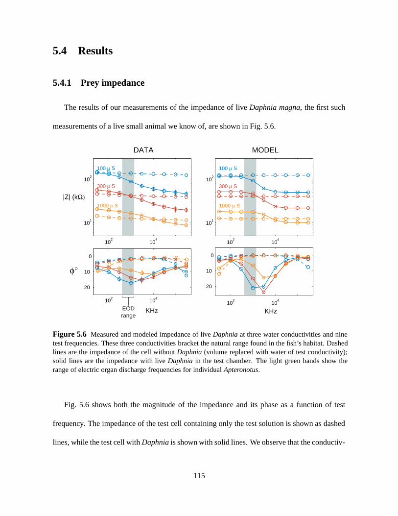
The results of our measurements of the impedance of liveDaphnia magna, thefirst such

measurements of a live small animal we know of, are shown in Fig. 5.6.

102

104

101

102

102

104

20

10

0

φ°

100 µ S

300 µ S

KHz

|Z| (kΩ)

KHz

102

104

101

102

102 104

20

10

0

freq (Hz)

100 µ S

300 µ S

1000 µ S 1000 µ S

EODrange

MODELDATA

Figure 5.6 Measured and modeled impedance of liveDaphnia at three water conductivities and ninetest frequencies. These three conductivities bracket the natural range found in thefish’s habitat. Dashedlines are the impedance of the cell withoutDaphnia (volume replaced with water of test conductivity);solid lines are the impedance with liveDaphnia in the test chamber. The light green bands show therange of electric organ discharge frequencies for individualApteronotus.

Fig. 5.6 shows both the magnitude of the impedance and its phase as a function of test

frequency. The impedance of the test cell containing only the test solution is shown as dashed

lines, while the test cell withDaphnia is shown with solid lines. We observe that the conductiv-

115

1000S, the highest value used in these measurements, he found thatfish were unable to make

discriminations on the basis of capacitance; he hypothesized that this was due to a reduction in

EOD amplitude at high conductivities (the EOD becomes effectively shorted at higher conduc-

tivity). We can see from Fig. 5.6 that the extent of the phase lag withDaphnia in the cell also

decreases with increasing conductivity of the external milieu. This may thus contribute to the

failure to discriminate capacitance in high conductivity water.

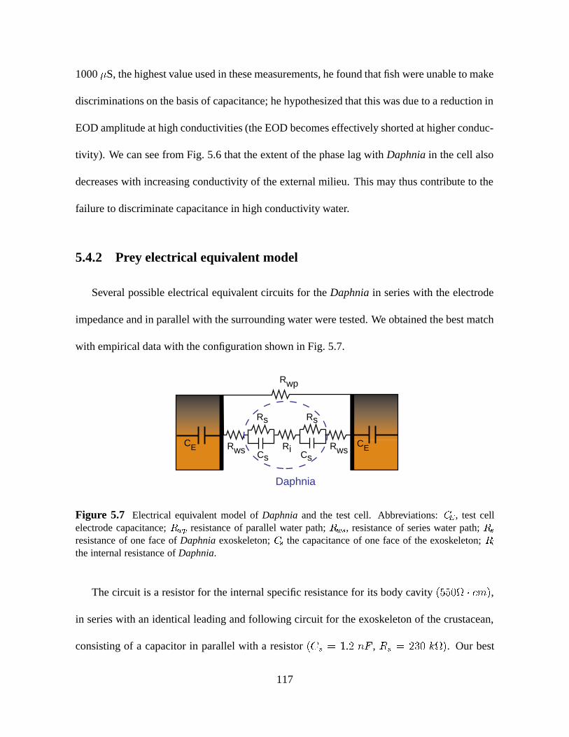
5.4.2 Prey electrical equivalent model

Several possible electrical equivalent circuits for theDaphnia in series with the electrode

impedance and in parallel with the surrounding water were tested. We obtained the best match

with empirical data with the configuration shown in Fig. 5.7.

Rwp

RwsRws

Rs Rs

Cs CsRi

CE CE

Daphnia

Figure 5.7 Electrical equivalent model ofDaphnia and the test cell. Abbreviations:CE, test cellelectrode capacitance;Rwp resistance of parallel water path;Rws, resistance of series water path;Rs

resistance of one face ofDaphnia exoskeleton;Cs the capacitance of one face of the exoskeleton;Rithe internal resistance ofDaphnia.

The circuit is a resistor for the internal specific resistance for its body cavity(550 cm),

in series with an identical leading and following circuit for the exoskeleton of the crustacean,

consisting of a capacitor in parallel with a resistor(Cs = 1:2 nF , Rs = 230 k). Our best

117

Tuberous Ampullary Lateral Line

No Treatment

24 Hr 0.1 mM Co++

1 Wk 0.1 mM Co++

Tuberous

gain, Hz/mV gain, Hz/mV response power, db

N = 18

0 1000 2000 30000

5

10

N = 12

0 1000 2000 30000

5

10

15

N = 8

0 1000 2000 30000

5

10

N = 9

0 20 40 600

1

2

3

N = 6

0 20 40 600

5

10

N = 9

0 20 40 600

5

10

N = 99

0 1000 2000 3000 40000

10

20

30

N = 16

0 1000 2000 3000 40000

5

10

N = 18

0 1000 2000 3000 40000

5

10

nu

mb

er o

f u

nit

sn

um

ber

of

un

its

nu

mb

er o

f u

nit

s

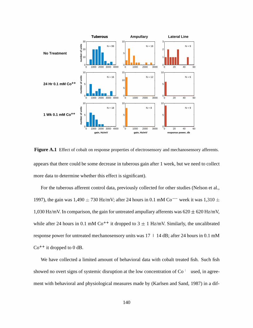
Figure A.1 Effect of cobalt on response properties of electrosensory and mechanosensory afferents.

appears that there could be some decrease in tuberous gain after 1 week, but we need to collect

more data to determine whether this effect is significant).

For the tuberous afferent control data, previously collected for other studies (Nelson et al.,

1997), the gain was 1,490 730 Hz/mV; after 24 hours in 0.1 mM Co++ week it was 1,310

1,030 Hz/mV. In comparison, the gain for untreated ampullary afferents was 620 620 Hz/mV,

while after 24 hours in 0.1 mM Co++ it dropped to 3 1 Hz/mV. Similarly, the uncalibrated

response power for untreated mechanosensory units was 17 14 dB; after 24 hours in 0.1 mM

Co++ it dropped to 0 dB.

We have collected a limited amount of behavioral data with cobalt treated fish. Such fish

showed no overt signs of systemic disruption at the low concentration of Co++ used, in agree-

ment with behavioral and physiological measures made by (Karlsen and Sand, 1987) in a dif-

140

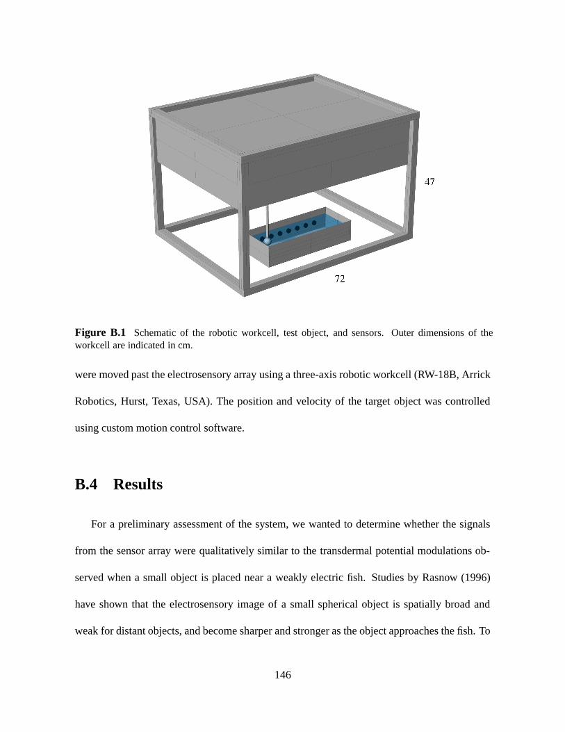
Figure B.1 Schematic of the robotic workcell, test object, and sensors. Outer dimensions of theworkcell are indicated in cm.

were moved past the electrosensory array using a three-axis robotic workcell (RW-18B, Arrick

Robotics, Hurst, Texas, USA). The position and velocity of the target object was controlled

using custom motion control software.

B.4 Results

For a preliminary assessment of the system, we wanted to determine whether the signals

from the sensor array were qualitatively similar to the transdermal potential modulations ob-

served when a small object is placed near a weakly electric fish. Studies by Rasnow (1996)

have shown that the electrosensory image of a small spherical object is spatially broad and

weak for distant objects, and become sharper and stronger as the object approaches the fish. To

146