The Central Curve in Linear ProgrammingThe Central Curve in Linear Programming Cynthia Vinzant, UC...
59
The Central Curve in Linear Programming Cynthia Vinzant, UC Berkeley → joint work with Jes´ us De Loera and Bernd Sturmfels Cynthia Vinzant, UC Berkeley The Central Curve in Linear Programming
Transcript of The Central Curve in Linear ProgrammingThe Central Curve in Linear Programming Cynthia Vinzant, UC...
The Central Curve in Linear Programming
Cynthia Vinzant, UC Berkeley
→
joint work with Jesus De Loera and Bernd Sturmfels
Cynthia Vinzant, UC Berkeley The Central Curve in Linear Programming

The Central Path of a Linear Program
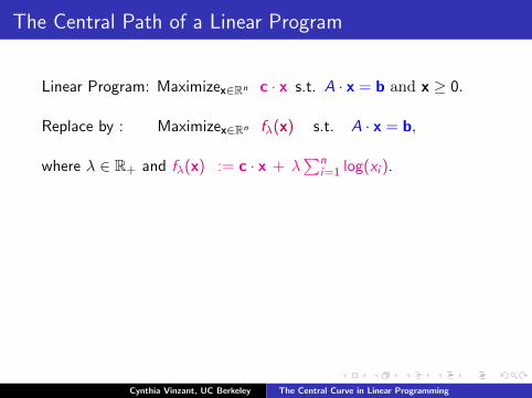
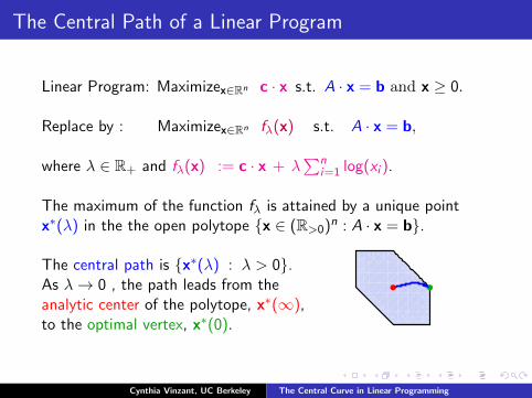
Linear Program: Maximizex∈Rn c · x s.t. A · x = b and x ≥ 0.
Replace by : Maximizex∈Rn fλ(x) s.t. A · x = b,
where λ ∈ R+ and fλ(x) := c · x + λ∑n
i=1 log(xi ).
The maximum of the function fλ is attained by a unique pointx∗(λ) in the the open polytope {x ∈ (R>0)n : A · x = b}.
The central path is {x∗(λ) : λ > 0}.As λ→ 0 , the path leads from theanalytic center of the polytope, x∗(∞),to the optimal vertex, x∗(0).
Cynthia Vinzant, UC Berkeley The Central Curve in Linear Programming
The Central Path of a Linear Program
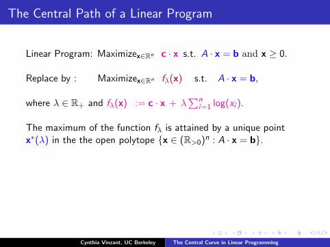
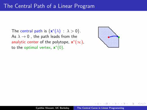
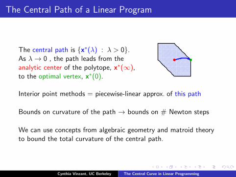
The central path is {x∗(λ) : λ > 0}.As λ→ 0 , the path leads from theanalytic center of the polytope, x∗(∞),to the optimal vertex, x∗(0).
Interior point methods = piecewise-linear approx. of this path
Bounds on curvature of the path → bounds on # Newton steps
We can use concepts from algebraic geometry and matroid theoryto bound the total curvature of the central path.
Cynthia Vinzant, UC Berkeley The Central Curve in Linear Programming
The Central Path of a Linear Program
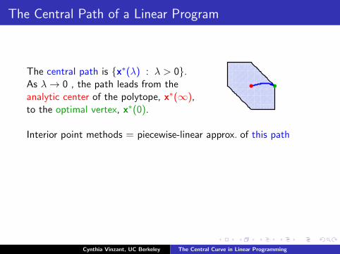
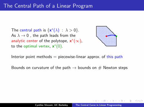
The central path is {x∗(λ) : λ > 0}.As λ→ 0 , the path leads from theanalytic center of the polytope, x∗(∞),to the optimal vertex, x∗(0).
Interior point methods = piecewise-linear approx. of this path
Bounds on curvature of the path → bounds on # Newton steps
We can use concepts from algebraic geometry and matroid theoryto bound the total curvature of the central path.
Cynthia Vinzant, UC Berkeley The Central Curve in Linear Programming
The Central Curve
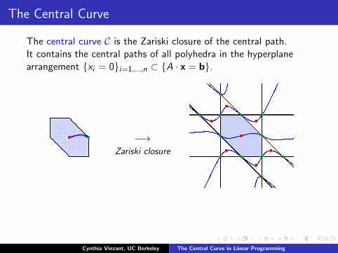
The central curve C is the Zariski closure of the central path.It contains the central paths of all polyhedra in the hyperplanearrangement {xi = 0}i=1,...,n ⊂ {A · x = b}.
−→Zariski closure
Goal: Study the nice algebraic geometry of this curveand its applications to the linear program
Cynthia Vinzant, UC Berkeley The Central Curve in Linear Programming
The Central Curve
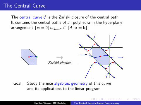
The central curve C is the Zariski closure of the central path.It contains the central paths of all polyhedra in the hyperplanearrangement {xi = 0}i=1,...,n ⊂ {A · x = b}.
−→Zariski closure
Goal: Study the nice algebraic geometry of this curveand its applications to the linear program
Cynthia Vinzant, UC Berkeley The Central Curve in Linear Programming

History and Contributions
Motivating Question: What is the maximum total curvature of thecentral path given the size of the matrix A?
Deza-Terlaky-Zinchenko (2008) make continuous Hirsch conjectureConjecture: The total curvature of the central path is at most O(n).
Bayer-Lagarias (1989) study the central path as an algebraic object andsuggest the problem of identifying its defining equations.
Dedieu-Malajovich-Shub (2005) apply differential and algebraic geometryto bound the total curvature of the central path.
Our contribution is to use results from algebraic geometry and matroid
theory to find defining equations of the central curve and refine bounds
on its degree and total curvature.
Cynthia Vinzant, UC Berkeley The Central Curve in Linear Programming
Outline
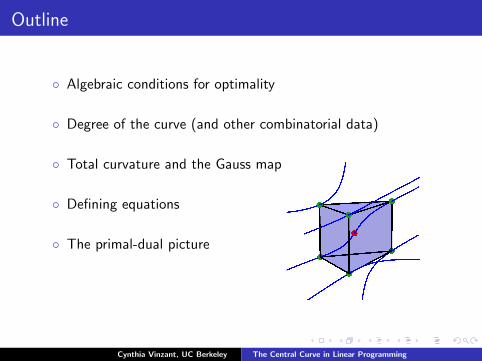
◦ Algebraic conditions for optimality
◦ Degree of the curve (and other combinatorial data)
◦ Total curvature and the Gauss map
◦ Defining equations
◦ The primal-dual picture
Cynthia Vinzant, UC Berkeley The Central Curve in Linear Programming

Some details
Here we assume that . . .
1) A is a d × n matrix of rank-d (possibly very special), and
2) c ∈ Rn and b ∈ Rd are generic.
(This ensures that the central curve is irreducible and nonsingular.)
Cynthia Vinzant, UC Berkeley The Central Curve in Linear Programming
Algebraic Conditions for Optimality
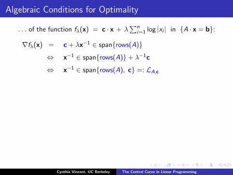
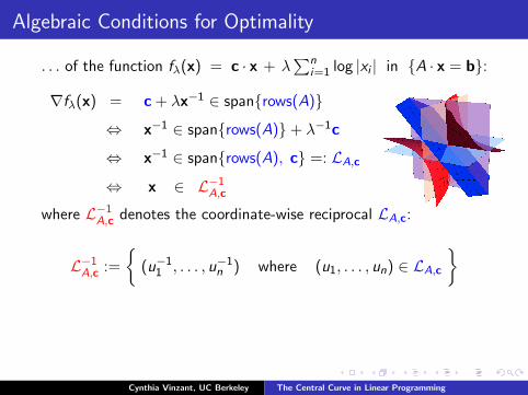
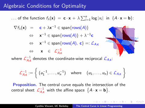
. . . of the function fλ(x) = c · x + λ∑n
i=1 log |xi | in {A · x = b}:
∇fλ(x) = c + λx−1 ∈ span{rows(A)}
⇔ x−1 ∈ span{rows(A)}+ λ−1c
⇔ x−1 ∈ span{rows(A), c} =: LA,c⇔ x ∈ L−1A,c
where L−1A,c denotes the coordinate-wise reciprocal LA,c:
L−1A,c :=
{(u−11 , . . . , u−1n ) where (u1, . . . , un) ∈ LA,c
}Proposition. The central curve equals the intersection of the
central sheet L−1A,c with the affine space{A · x = b
}.
Cynthia Vinzant, UC Berkeley The Central Curve in Linear Programming
Algebraic Conditions for Optimality
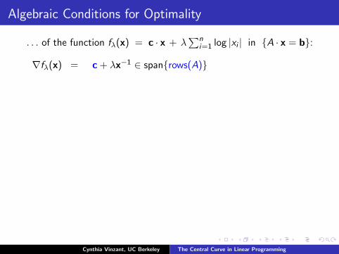
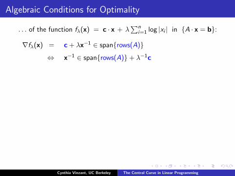
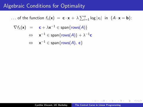
. . . of the function fλ(x) = c · x + λ∑n
i=1 log |xi | in {A · x = b}:
∇fλ(x) = c + λx−1 ∈ span{rows(A)}
⇔ x−1 ∈ span{rows(A)}+ λ−1c
⇔ x−1 ∈ span{rows(A), c}
=: LA,c⇔ x ∈ L−1A,c
where L−1A,c denotes the coordinate-wise reciprocal LA,c:
L−1A,c :=
{(u−11 , . . . , u−1n ) where (u1, . . . , un) ∈ LA,c
}Proposition. The central curve equals the intersection of the
central sheet L−1A,c with the affine space{A · x = b
}.
Cynthia Vinzant, UC Berkeley The Central Curve in Linear Programming
Algebraic Conditions for Optimality
. . . of the function fλ(x) = c · x + λ∑n
i=1 log |xi | in {A · x = b}:
∇fλ(x) = c + λx−1 ∈ span{rows(A)}
⇔ x−1 ∈ span{rows(A)}+ λ−1c
⇔ x−1 ∈ span{rows(A), c} =: LA,c
⇔ x ∈ L−1A,c
where L−1A,c denotes the coordinate-wise reciprocal LA,c:
L−1A,c :=
{(u−11 , . . . , u−1n ) where (u1, . . . , un) ∈ LA,c
}Proposition. The central curve equals the intersection of the
central sheet L−1A,c with the affine space{A · x = b
}.
Cynthia Vinzant, UC Berkeley The Central Curve in Linear Programming
Algebraic Conditions for Optimality
. . . of the function fλ(x) = c · x + λ∑n
i=1 log |xi | in {A · x = b}:
∇fλ(x) = c + λx−1 ∈ span{rows(A)}
⇔ x−1 ∈ span{rows(A)}+ λ−1c
⇔ x−1 ∈ span{rows(A), c} =: LA,c⇔ x ∈ L−1A,c
where L−1A,c denotes the coordinate-wise reciprocal LA,c:
L−1A,c :=
{(u−11 , . . . , u−1n ) where (u1, . . . , un) ∈ LA,c
}
Proposition. The central curve equals the intersection of thecentral sheet L−1A,c with the affine space
{A · x = b
}.
Cynthia Vinzant, UC Berkeley The Central Curve in Linear Programming
Algebraic Conditions for Optimality
. . . of the function fλ(x) = c · x + λ∑n
i=1 log |xi | in {A · x = b}:
∇fλ(x) = c + λx−1 ∈ span{rows(A)}
⇔ x−1 ∈ span{rows(A)}+ λ−1c
⇔ x−1 ∈ span{rows(A), c} =: LA,c⇔ x ∈ L−1A,c
where L−1A,c denotes the coordinate-wise reciprocal LA,c:
L−1A,c :=
{(u−11 , . . . , u−1n ) where (u1, . . . , un) ∈ LA,c
}Proposition. The central curve equals the intersection of the
central sheet L−1A,c with the affine space{A · x = b
}.
Cynthia Vinzant, UC Berkeley The Central Curve in Linear Programming
Level sets of the cost function
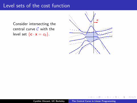
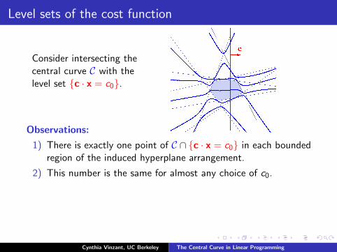
Consider intersecting thecentral curve C with thelevel set {c · x = c0}.
Observations:
1) There is exactly one point of C ∩ {c · x = c0} in each boundedregion of the induced hyperplane arrangement.
2) This number is the same for almost any choice of c0.
Claim: The points C ∩ {c · x = c0} are the analytic centers of thehyperplane arrangement {xi = 0}i∈[n] in {A · x = b, c · x = c0}.
Cynthia Vinzant, UC Berkeley The Central Curve in Linear Programming
Level sets of the cost function
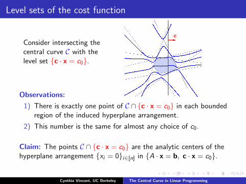
Consider intersecting thecentral curve C with thelevel set {c · x = c0}.
Observations:
1) There is exactly one point of C ∩ {c · x = c0} in each boundedregion of the induced hyperplane arrangement.
2) This number is the same for almost any choice of c0.
Claim: The points C ∩ {c · x = c0} are the analytic centers of thehyperplane arrangement {xi = 0}i∈[n] in {A · x = b, c · x = c0}.
Cynthia Vinzant, UC Berkeley The Central Curve in Linear Programming
Level sets of the cost function and analytic centers
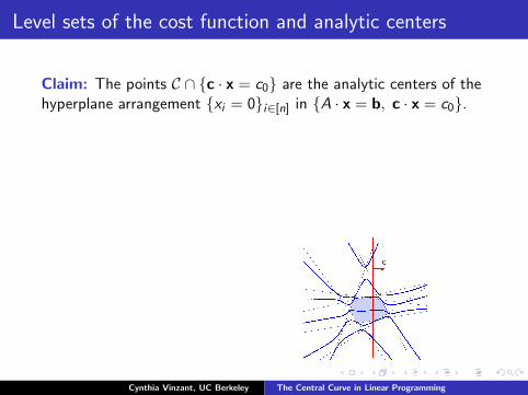
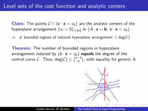
Claim: The points C ∩ {c · x = c0} are the analytic centers of thehyperplane arrangement {xi = 0}i∈[n] in {A · x = b, c · x = c0}.
⇒ # bounded regions of induced hyperplane arrangement ≤ deg(C)
Theorem: The number of bounded regions in hyperplanearrangement induced by {c · x = c0} equals the degree of thecentral curve C. Thus, deg(C) ≤
(n−1d
), with equality for generic A.
For matroid enthusiasts,
this number is the absolute value
of the Mobius invariant of(Ac
).
Cynthia Vinzant, UC Berkeley The Central Curve in Linear Programming
Level sets of the cost function and analytic centers
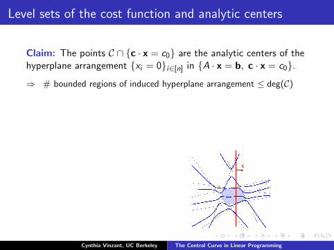
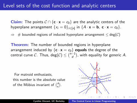
Claim: The points C ∩ {c · x = c0} are the analytic centers of thehyperplane arrangement {xi = 0}i∈[n] in {A · x = b, c · x = c0}.
⇒ # bounded regions of induced hyperplane arrangement ≤ deg(C)
Theorem: The number of bounded regions in hyperplanearrangement induced by {c · x = c0} equals the degree of thecentral curve C. Thus, deg(C) ≤
(n−1d
), with equality for generic A.
For matroid enthusiasts,
this number is the absolute value
of the Mobius invariant of(Ac
).
Cynthia Vinzant, UC Berkeley The Central Curve in Linear Programming
Level sets of the cost function and analytic centers
Claim: The points C ∩ {c · x = c0} are the analytic centers of thehyperplane arrangement {xi = 0}i∈[n] in {A · x = b, c · x = c0}.
⇒ # bounded regions of induced hyperplane arrangement ≤ deg(C)
Theorem: The number of bounded regions in hyperplanearrangement induced by {c · x = c0} equals the degree of thecentral curve C. Thus, deg(C) ≤
(n−1d
), with equality for generic A.
For matroid enthusiasts,
this number is the absolute value
of the Mobius invariant of(Ac
).
Cynthia Vinzant, UC Berkeley The Central Curve in Linear Programming
Combinatorial data
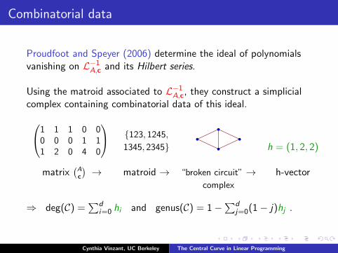
Proudfoot and Speyer (2006) determine the ideal of polynomialsvanishing on L−1A,c and its Hilbert series.
Using the matroid associated to L−1A,c, they construct a simplicialcomplex containing combinatorial data of this ideal.
1 1 1 0 00 0 0 1 11 2 0 4 0
{123, 1245,
1345, 2345} h = (1, 2, 2)
matrix(Ac
)→ matroid → “broken circuit” → h-vector
complex
⇒ deg(C) =∑d
i=0 hi and genus(C) = 1−∑d
j=0(1− j)hj .
Cynthia Vinzant, UC Berkeley The Central Curve in Linear Programming
Combinatorial data
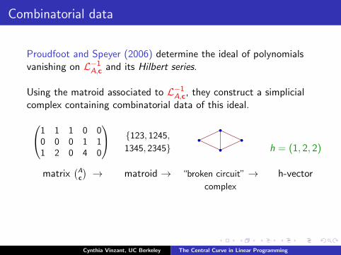
Proudfoot and Speyer (2006) determine the ideal of polynomialsvanishing on L−1A,c and its Hilbert series.
Using the matroid associated to L−1A,c, they construct a simplicialcomplex containing combinatorial data of this ideal.
1 1 1 0 00 0 0 1 11 2 0 4 0
{123, 1245,
1345, 2345} h = (1, 2, 2)
matrix(Ac
)→ matroid → “broken circuit” → h-vector
complex
⇒ deg(C) =∑d
i=0 hi and genus(C) = 1−∑d
j=0(1− j)hj .
Cynthia Vinzant, UC Berkeley The Central Curve in Linear Programming

Total Curvature
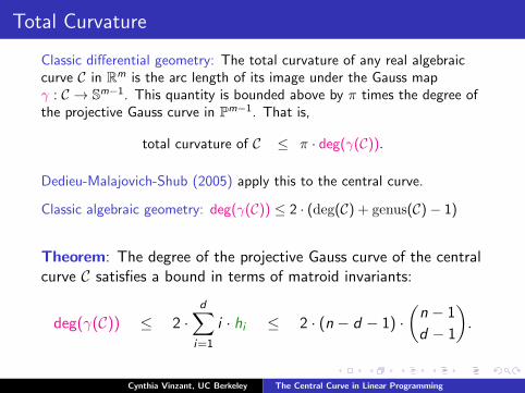
Classic differential geometry: The total curvature of any real algebraiccurve C in Rm is the arc length of its image under the Gauss mapγ : C → Sm−1. This quantity is bounded above by π times the degree ofthe projective Gauss curve in Pm−1. That is,
total curvature of C ≤ π · deg(γ(C)).
Dedieu-Malajovich-Shub (2005) apply this to the central curve.
Classic algebraic geometry: deg(γ(C)) ≤ 2 · (deg(C) + genus(C)− 1)
Theorem: The degree of the projective Gauss curve of the centralcurve C satisfies a bound in terms of matroid invariants:
deg(γ(C)) ≤ 2 ·d∑
i=1
i · hi ≤ 2 · (n − d − 1) ·(n − 1
d − 1
).
Cynthia Vinzant, UC Berkeley The Central Curve in Linear Programming

Total Curvature
Classic differential geometry: The total curvature of any real algebraiccurve C in Rm is the arc length of its image under the Gauss mapγ : C → Sm−1. This quantity is bounded above by π times the degree ofthe projective Gauss curve in Pm−1. That is,
total curvature of C ≤ π · deg(γ(C)).
Dedieu-Malajovich-Shub (2005) apply this to the central curve.
Classic algebraic geometry: deg(γ(C)) ≤ 2 · (deg(C) + genus(C)− 1)
Theorem: The degree of the projective Gauss curve of the centralcurve C satisfies a bound in terms of matroid invariants:
deg(γ(C)) ≤ 2 ·d∑
i=1
i · hi ≤ 2 · (n − d − 1) ·(n − 1
d − 1
).
Cynthia Vinzant, UC Berkeley The Central Curve in Linear Programming
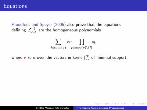
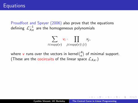
Equations
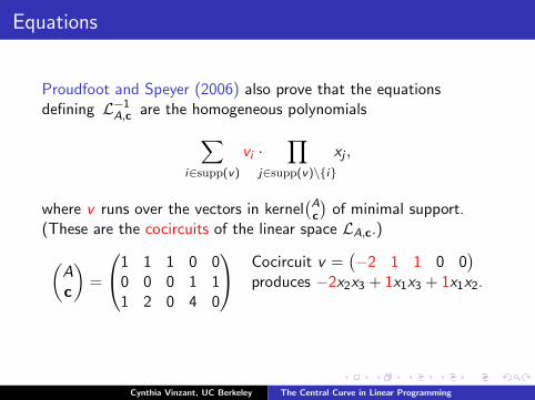
Proudfoot and Speyer (2006) also prove that the equationsdefining L−1A,c are the homogeneous polynomials∑
i∈supp(v)
vi ·∏
j∈supp(v)\{i}
xj ,
where v runs over the vectors in kernel(Ac
)of minimal support.
(These are the cocircuits of the linear space LA,c.)
(Ac
)=
1 1 1 0 00 0 0 1 11 2 0 4 0
Cocircuit v =(−2 1 1 0 0
)produces −2x2x3 + 1x1x3 + 1x1x2.
Cynthia Vinzant, UC Berkeley The Central Curve in Linear Programming
Equations
Proudfoot and Speyer (2006) also prove that the equationsdefining L−1A,c are the homogeneous polynomials∑
i∈supp(v)
vi ·∏
j∈supp(v)\{i}
xj ,
where v runs over the vectors in kernel(Ac
)of minimal support.
(These are the cocircuits of the linear space LA,c.)
(Ac
)=
1 1 1 0 00 0 0 1 11 2 0 4 0
Cocircuit v =(−2 1 1 0 0
)produces −2x2x3 + 1x1x3 + 1x1x2.
Cynthia Vinzant, UC Berkeley The Central Curve in Linear Programming
Example
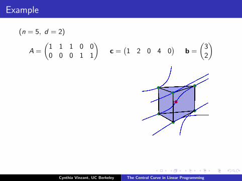
(n = 5, d = 2)
A =
(1 1 1 0 00 0 0 1 1
)c =
(1 2 0 4 0
)b =
(32
)
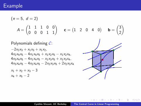
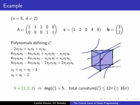
Polynomials defining C:
−2x2x3 + x1x3 + x1x2,4x2x4x5 − 4x1x4x5 + x1x2x5 − x1x2x4,4x3x4x5 − 4x1x4x5 − x1x3x5 + x1x3x4,4x3x4x5 − 4x2x4x5 − 2x2x3x5 + 2x2x3x4
x1 + x2 + x3 − 3
x4 + x5 − 2
h = (1, 2, 2) ⇒ deg(C) = 5, total curvature(C) ≤ 12π
(≤ 16π)
Cynthia Vinzant, UC Berkeley The Central Curve in Linear Programming
Example
(n = 5, d = 2)
A =
(1 1 1 0 00 0 0 1 1
)c =
(1 2 0 4 0
)b =
(32
)Polynomials defining C:
−2x2x3 + x1x3 + x1x2,4x2x4x5 − 4x1x4x5 + x1x2x5 − x1x2x4,4x3x4x5 − 4x1x4x5 − x1x3x5 + x1x3x4,4x3x4x5 − 4x2x4x5 − 2x2x3x5 + 2x2x3x4
x1 + x2 + x3 − 3
x4 + x5 − 2
h = (1, 2, 2) ⇒ deg(C) = 5, total curvature(C) ≤ 12π
(≤ 16π)
Cynthia Vinzant, UC Berkeley The Central Curve in Linear Programming
Example
(n = 5, d = 2)
A =
(1 1 1 0 00 0 0 1 1
)c =
(1 2 0 4 0
)b =
(32
)Polynomials defining C:
−2x2x3 + x1x3 + x1x2,4x2x4x5 − 4x1x4x5 + x1x2x5 − x1x2x4,4x3x4x5 − 4x1x4x5 − x1x3x5 + x1x3x4,4x3x4x5 − 4x2x4x5 − 2x2x3x5 + 2x2x3x4
x1 + x2 + x3 − 3
x4 + x5 − 2
h = (1, 2, 2) ⇒ deg(C) = 5, total curvature(C) ≤ 12π (≤ 16π)
Cynthia Vinzant, UC Berkeley The Central Curve in Linear Programming

Duality
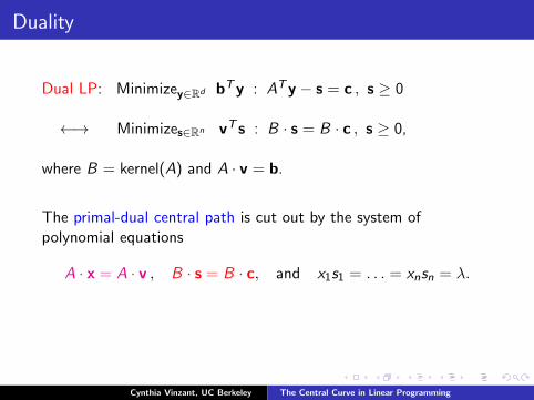
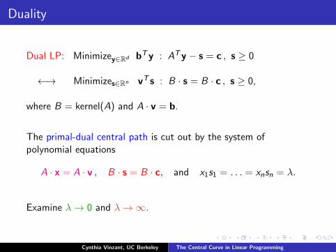
Dual LP: Minimizey∈Rd bTy : ATy − s = c , s ≥ 0
←→ Minimizes∈Rn vT s : B · s = B · c , s ≥ 0,
where B = kernel(A) and A · v = b.
The primal-dual central path is cut out by the system ofpolynomial equations
A · x = A · v , B · s = B · c, and x1s1 = . . . = xnsn = λ.
Examine λ→ 0 and λ→∞.
Cynthia Vinzant, UC Berkeley The Central Curve in Linear Programming
Duality
Dual LP: Minimizey∈Rd bTy : ATy − s = c , s ≥ 0
←→ Minimizes∈Rn vT s : B · s = B · c , s ≥ 0,
where B = kernel(A) and A · v = b.
The primal-dual central path is cut out by the system ofpolynomial equations
A · x = A · v , B · s = B · c, and x1s1 = . . . = xnsn = λ.
Examine λ→ 0 and λ→∞.
Cynthia Vinzant, UC Berkeley The Central Curve in Linear Programming
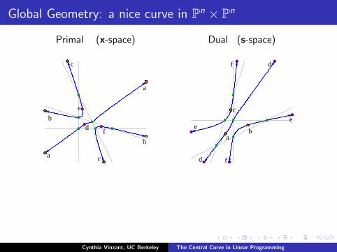
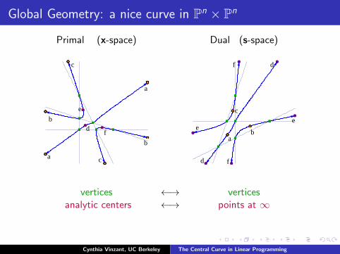
Global Geometry: a nice curve in Pn × Pn
Primal (x-space) Dual (s-space)
a
b
b
a
c
c
f
e
de
e
f d
fd
b
c
a
vertices ←→ verticesanalytic centers ←→ points at ∞
points at ∞ ←→ analytic centers
Cynthia Vinzant, UC Berkeley The Central Curve in Linear Programming
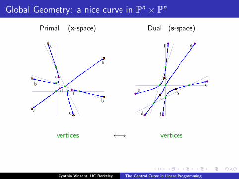
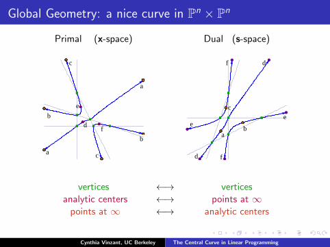
Global Geometry: a nice curve in Pn × Pn
Primal (x-space) Dual (s-space)
a
b
b
a
c
c
f
e
de
e
f d
fd
b
c
a
vertices ←→ vertices
analytic centers ←→ points at ∞points at ∞ ←→ analytic centers
Cynthia Vinzant, UC Berkeley The Central Curve in Linear Programming
Global Geometry: a nice curve in Pn × Pn
Primal (x-space) Dual (s-space)
a
b
b
a
c
c
f
e
de
e
f d
fd
b
c
a
vertices ←→ verticesanalytic centers ←→ points at ∞
points at ∞ ←→ analytic centers
Cynthia Vinzant, UC Berkeley The Central Curve in Linear Programming
Global Geometry: a nice curve in Pn × Pn
Primal (x-space) Dual (s-space)
a
b
b
a
c
c
f
e
de
e
f d
fd
b
c
a
vertices ←→ verticesanalytic centers ←→ points at ∞
points at ∞ ←→ analytic centers
Cynthia Vinzant, UC Berkeley The Central Curve in Linear Programming
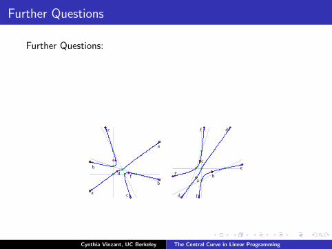
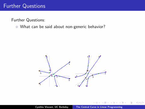
Further Questions
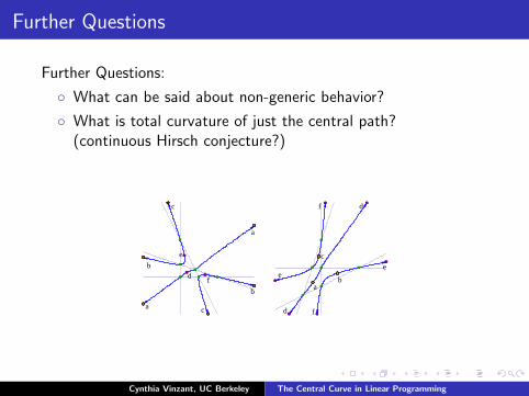
Further Questions:
◦ What can be said about non-generic behavior?
◦ What is total curvature of just the central path?(continuous Hirsch conjecture?)
◦ Extensions to semidefinite and hyperbolic programs?
a
b
b
a
c
c
f
e
de
e
f d
fd
b
c
a
Thanks!
Cynthia Vinzant, UC Berkeley The Central Curve in Linear Programming
Further Questions
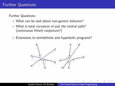
Further Questions:
◦ What can be said about non-generic behavior?
◦ What is total curvature of just the central path?(continuous Hirsch conjecture?)
◦ Extensions to semidefinite and hyperbolic programs?
a
b
b
a
c
c
f
e
de
e
f d
fd
b
c
a
Thanks!
Cynthia Vinzant, UC Berkeley The Central Curve in Linear Programming
Further Questions
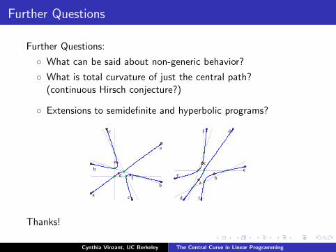
Further Questions:
◦ What can be said about non-generic behavior?
◦ What is total curvature of just the central path?(continuous Hirsch conjecture?)
◦ Extensions to semidefinite and hyperbolic programs?
a
b
b
a
c
c
f
e
de
e
f d
fd
b
c
a
Thanks!
Cynthia Vinzant, UC Berkeley The Central Curve in Linear Programming
Further Questions
Further Questions:
◦ What can be said about non-generic behavior?
◦ What is total curvature of just the central path?(continuous Hirsch conjecture?)
◦ Extensions to semidefinite and hyperbolic programs?
a
b
b
a
c
c
f
e
de
e
f d
fd
b
c
a
Thanks!
Cynthia Vinzant, UC Berkeley The Central Curve in Linear Programming