The Calderon problem with partial data

Mikko SaloUniversity of Jyvaskyla

Harmonic analysis & PDEConference in honor of Carlos Kenig

Chicago, September 20, 2014

fiFinnish Centre of Excellence

in Inverse Problems Research

Calderon problem

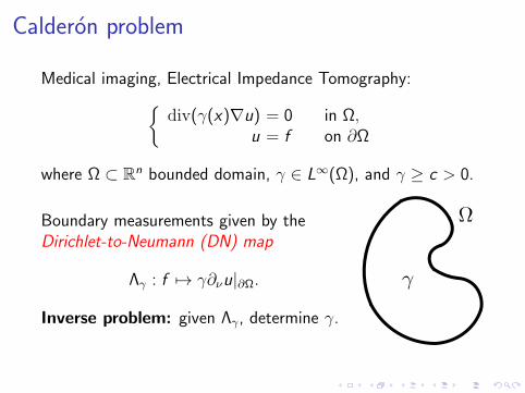
Medical imaging, Electrical Impedance Tomography:

div(γ(x)∇u) = 0 in Ω,

u = f on ∂Ω

where Ω ⊂ Rn bounded domain, γ ∈ L∞(Ω), and γ ≥ c > 0.

Boundary measurements given by theDirichlet-to-Neumann (DN) map

Λγ : f 7→ γ∂νu|∂Ω.

Inverse problem: given Λγ, determine γ.

Calderon problem

Model case of inverse boundary problems for elliptic equations(Schrodinger, Maxwell, elasticity).

Related to:

optical tomography

inverse scattering

travel time tomography and boundary rigidity

hybrid imaging methods

invisibility

Calderon’s approach

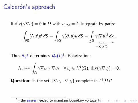
If div(γ∇u) = 0 in Ω with u|∂Ω = f , integrate by parts:

∫

∂Ω

(Λγf )f dS =

∫

∂Ω

γ(∂νu)u dS =

∫

Ω

γ|∇u|2 dx

︸ ︷︷ ︸

=:Qγ(f )

.

Thus Λγf determines Qγ(f )1. Polarization:

Λγ !

∫

Ω

γ∇u1 · ∇u2 ∀ uj ∈ H1(Ω), div(γ∇uj) = 0.

Question: is the set ∇u1 · ∇u2 complete in L1(Ω)?

1=the power needed to maintain boundary voltage f

Calderon’s approach

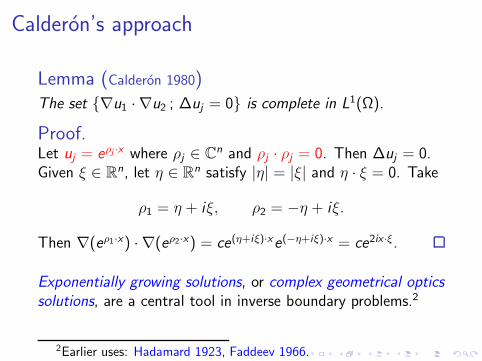
Lemma (Calderon 1980)The set ∇u1 · ∇u2 ; ∆uj = 0 is complete in L1(Ω).

Proof.Let uj = eρj ·x where ρj ∈ C

n and ρj · ρj = 0. Then ∆uj = 0.Given ξ ∈ Rn, let η ∈ Rn satisfy |η| = |ξ| and η · ξ = 0. Take

ρ1 = η + iξ, ρ2 = −η + iξ.

Then ∇(eρ1·x) · ∇(eρ2·x) = ce(η+iξ)·xe(−η+iξ)·x = ce2ix ·ξ.

Exponentially growing solutions, or complex geometrical opticssolutions, are a central tool in inverse boundary problems.2

2Earlier uses: Hadamard 1923, Faddeev 1966.

Calderon problem

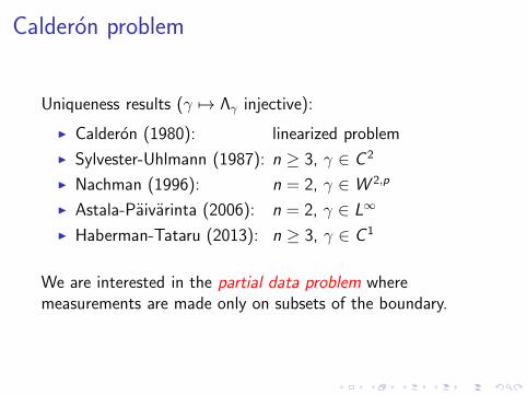
Uniqueness results (γ 7→ Λγ injective):

Calderon (1980): linearized problem

Sylvester-Uhlmann (1987): n ≥ 3, γ ∈ C 2

Nachman (1996): n = 2, γ ∈ W 2,p

Astala-Paivarinta (2006): n = 2, γ ∈ L∞

Haberman-Tataru (2013): n ≥ 3, γ ∈ C 1

We are interested in the partial data problem wheremeasurements are made only on subsets of the boundary.

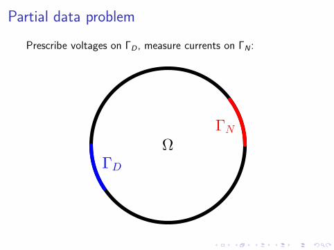
Partial data problem

Prescribe voltages on ΓD , measure currents on ΓN :

Partial data problem

Particular case (local data problem): ΓD = ΓN = Γ.

Uniqueness known for arbitrary open Γ ⊂ ∂Ω

if n = 2

for piecewise real-analytic conductivities if n ≥ 3.

Open in general if n ≥ 3. This talk will survey known results.

Partial data problem

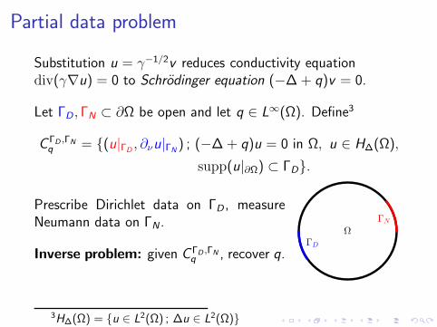
Substitution u = γ−1/2v reduces conductivity equationdiv(γ∇u) = 0 to Schrodinger equation (−∆+ q)v = 0.

Let ΓD , ΓN ⊂ ∂Ω be open and let q ∈ L∞(Ω). Define3

C ΓD ,ΓNq = (u|ΓD , ∂νu|ΓN ) ; (−∆+ q)u = 0 in Ω, u ∈ H∆(Ω),

supp(u|∂Ω) ⊂ ΓD.

Prescribe Dirichlet data on ΓD , measureNeumann data on ΓN .

Inverse problem: given C ΓD ,ΓNq , recover q.

3H∆(Ω) = u ∈ L2(Ω) ; ∆u ∈ L2(Ω)

Partial data problem

Four main approaches for uniqueness:

1. Carleman estimates (Kenig-Sjostrand-Uhlmann 2007)

2. Reflection approach (Isakov 2007)

3. 2D case (Imanuvilov-Uhlmann-Yamamoto 2010)

4. Linearized case (Dos Santos-Kenig-Sjostrand-Uhlmann 2009)

The first two approaches apply when n ≥ 3. Other results:

piecewise analytic conductivities (Kohn-Vogelius)

other equations (Dos Santos et al, Chung, Chung-S-Tzou)

stability (Heck-Wang, Caro-Dos Santos-Ruiz)

numerics (Garde-Knudsen, Hamilton-Siltanen)

Strategy of proof

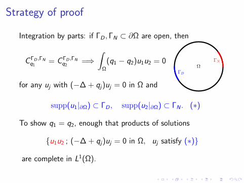
Integration by parts: if ΓD , ΓN ⊂ ∂Ω are open, then

C ΓD ,ΓNq1

= C ΓD ,ΓNq2

=⇒

∫

Ω

(q1 − q2)u1u2 = 0

for any uj with (−∆+ qj)uj = 0 in Ω and

supp(u1|∂Ω) ⊂ ΓD , supp(u2|∂Ω) ⊂ ΓN . (∗)

To show q1 = q2, enough that products of solutions

u1u2 ; (−∆+ qj)uj = 0 in Ω, uj satisfy (∗)

are complete in L1(Ω).

Strategy of proof

Use special complex geometrical optics solutions

u ≈ e±τϕa, (−∆+ q)u = 0, supp(u|∂Ω) ⊂ ΓD,N .

Here τ > 0 is a large parameter. Want to show that

limτ→∞

u1u2 dense in L1(Ω).

take u1 ≈ eτϕa1, u2 ≈ e−τϕa2 to kill exponential growthof limτ→∞ u1u2

correct approximate solution u0 = e±τϕa to exact solutionu = e±τϕ(a + r) by solving (−∆+ q)e±τϕ(a + r) = 0

possible if ϕ is a limiting Carleman weight

Strategy of proof

Condition for a limiting Carleman weight ϕ, ∇ϕ 6= 0:

‖v‖L2(Ω) ≤C

τ‖e±τϕ∆e∓τϕv‖L2(Ω), v ∈ C∞

c (Ω), τ ≫ 1.

Results from Dos Santos-Kenig-S-Uhlmann (2009):

conformally invariant condition

if n ≥ 3, only six basic forms for ϕ:

x1, log |x |,x1|x |2

, arctanx2x1, . . . .

if n = 2, any harmonic function is OK

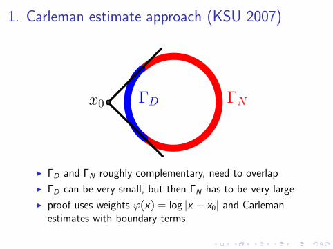
1. Carleman estimate approach (KSU 2007)

ΓD and ΓN roughly complementary, need to overlap

ΓD can be very small, but then ΓN has to be very large

proof uses weights ϕ(x) = log |x − x0| and Carlemanestimates with boundary terms

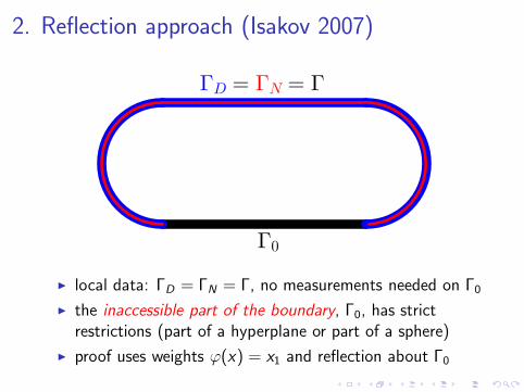
2. Reflection approach (Isakov 2007)

local data: ΓD = ΓN = Γ, no measurements needed on Γ0 the inaccessible part of the boundary, Γ0, has strict

restrictions (part of a hyperplane or part of a sphere)

proof uses weights ϕ(x) = x1 and reflection about Γ0

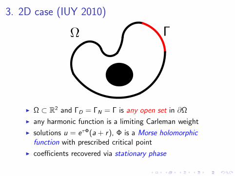
3. 2D case (IUY 2010)

Ω ⊂ R2 and ΓD = ΓN = Γ is any open set in ∂Ω

any harmonic function is a limiting Carleman weight

solutions u = eτΦ(a + r), Φ is a Morse holomorphicfunction with prescribed critical point

coefficients recovered via stationary phase

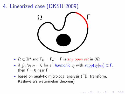
4. Linearized case (DKSU 2009)

Ω ⊂ Rn and ΓD = ΓN = Γ is any open set in ∂Ω

if∫

Ωfu1u2 = 0 for all harmonic uj with supp(uj |∂Ω) ⊂ Γ,

then f = 0 near Γ

based on analytic microlocal analysis (FBI transform,Kashiwara’s watermelon theorem)

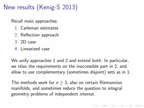
New results (Kenig-S 2013)

Recall main approaches:

1. Carleman estimates

2. Reflection approach

3. 2D case

4. Linearized case

We unify approaches 1 and 2 and extend both. In particular,we relax the requirements on the inaccessible part in 2, andallow to use complementary (sometimes disjoint) sets as in 1.

The methods work for n ≥ 3, also on certain Riemannianmanifolds, and sometimes reduce the question to integralgeometry problems of independent interest.

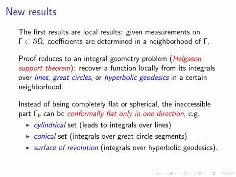
New results

The first results are local results: given measurements onΓ ⊂ ∂Ω, coefficients are determined in a neighborhood of Γ.

Proof reduces to an integral geometry problem (Helgasonsupport theorem): recover a function locally from its integralsover lines, great circles, or hyperbolic geodesics in a certainneighborhood.

Instead of being completely flat or spherical, the inaccessiblepart Γ0 can be conformally flat only in one direction, e.g.

cylindrical set (leads to integrals over lines)

conical set (integrals over great circle segments)

surface of revolution (integrals over hyperbolic geodesics).

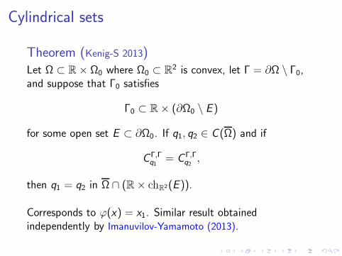
Cylindrical sets

Theorem (Kenig-S 2013)Let Ω ⊂ R× Ω0 where Ω0 ⊂ R2 is convex, let Γ = ∂Ω \ Γ0,and suppose that Γ0 satisfies

Γ0 ⊂ R× (∂Ω0 \ E )

for some open set E ⊂ ∂Ω0. If q1, q2 ∈ C (Ω) and if

C Γ,Γq1

= C Γ,Γq2

,

then q1 = q2 in Ω ∩ (R× chR2(E )).

Corresponds to ϕ(x) = x1. Similar result obtainedindependently by Imanuvilov-Yamamoto (2013).

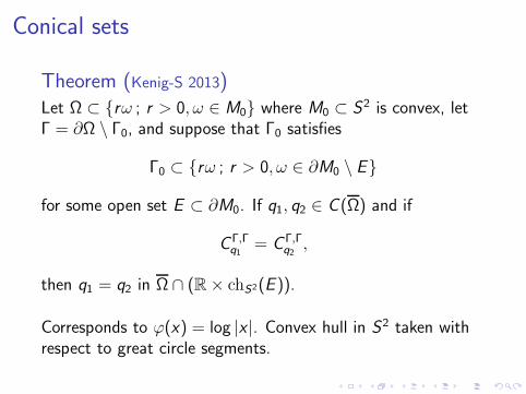
Conical sets

Theorem (Kenig-S 2013)Let Ω ⊂ rω ; r > 0, ω ∈ M0 where M0 ⊂ S2 is convex, letΓ = ∂Ω \ Γ0, and suppose that Γ0 satisfies

Γ0 ⊂ rω ; r > 0, ω ∈ ∂M0 \ E

for some open set E ⊂ ∂M0. If q1, q2 ∈ C (Ω) and if

C Γ,Γq1

= C Γ,Γq2

,

then q1 = q2 in Ω ∩ (R× chS2(E )).

Corresponds to ϕ(x) = log |x |. Convex hull in S2 taken withrespect to great circle segments.

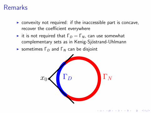
Remarks

convexity not required: if the inaccessible part is concave,recover the coefficient everywhere

it is not required that ΓD = ΓN , can use somewhatcomplementary sets as in Kenig-Sjostrand-Uhlmann

sometimes ΓD and ΓN can be disjoint

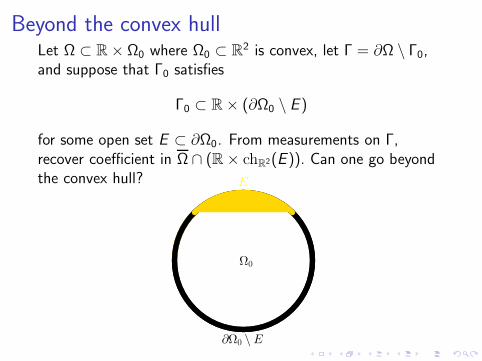
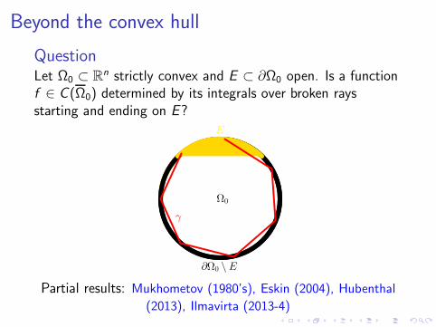
Beyond the convex hullLet Ω ⊂ R× Ω0 where Ω0 ⊂ R2 is convex, let Γ = ∂Ω \ Γ0,and suppose that Γ0 satisfies

Γ0 ⊂ R× (∂Ω0 \ E )

for some open set E ⊂ ∂Ω0. From measurements on Γ,recover coefficient in Ω ∩ (R× chR2(E )). Can one go beyondthe convex hull?

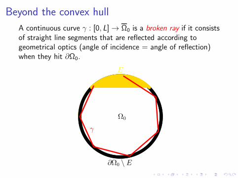
Beyond the convex hull

A continuous curve γ : [0, L] → Ω0 is a broken ray if it consistsof straight line segments that are reflected according togeometrical optics (angle of incidence = angle of reflection)when they hit ∂Ω0.

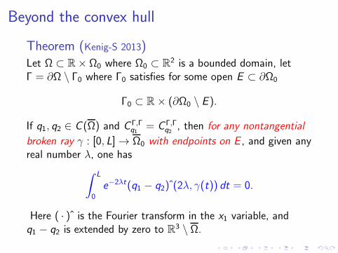
Beyond the convex hull

Theorem (Kenig-S 2013)Let Ω ⊂ R× Ω0 where Ω0 ⊂ R2 is a bounded domain, letΓ = ∂Ω \ Γ0 where Γ0 satisfies for some open E ⊂ ∂Ω0

Γ0 ⊂ R× (∂Ω0 \ E ).

If q1, q2 ∈ C (Ω) and C Γ,Γq1

= C Γ,Γq2

, then for any nontangential

broken ray γ : [0, L] → Ω0 with endpoints on E , and given anyreal number λ, one has

∫ L

0

e−2λt(q1 − q2) (2λ, γ(t)) dt = 0.

Here ( · ) is the Fourier transform in the x1 variable, andq1 − q2 is extended by zero to R3 \ Ω.

Beyond the convex hull

QuestionLet Ω0 ⊂ Rn strictly convex and E ⊂ ∂Ω0 open. Is a functionf ∈ C (Ω0) determined by its integrals over broken raysstarting and ending on E?

Partial results: Mukhometov (1980’s), Eskin (2004), Hubenthal

(2013), Ilmavirta (2013-4)

Components of proof

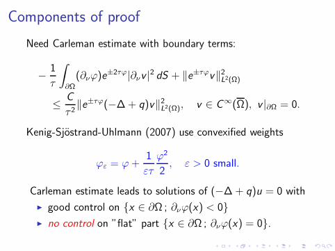
Need Carleman estimate with boundary terms:

−1

τ

∫

∂Ω

(∂νϕ)e±2τϕ|∂νv |

2 dS + ‖e±τϕv‖2L2(Ω)

≤C

τ 2‖e±τϕ(−∆+ q)v‖2L2(Ω), v ∈ C∞(Ω), v |∂Ω = 0.

Kenig-Sjostrand-Uhlmann (2007) use convexified weights

ϕε = ϕ+1

ετ

ϕ2

2, ε > 0 small.

Carleman estimate leads to solutions of (−∆+ q)u = 0 with

good control on x ∈ ∂Ω ; ∂νϕ(x) < 0

no control on ”flat” part x ∈ ∂Ω ; ∂νϕ(x) = 0.

Components of proof

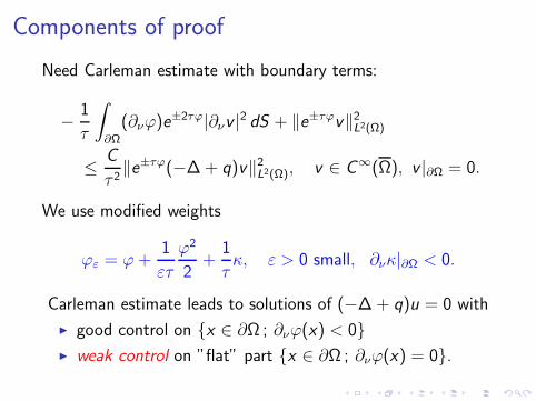
Need Carleman estimate with boundary terms:

−1

τ

∫

∂Ω

(∂νϕ)e±2τϕ|∂νv |

2 dS + ‖e±τϕv‖2L2(Ω)

≤C

τ 2‖e±τϕ(−∆+ q)v‖2L2(Ω), v ∈ C∞(Ω), v |∂Ω = 0.

We use modified weights

ϕε = ϕ+1

ετ

ϕ2

2+

1

τκ, ε > 0 small, ∂νκ|∂Ω < 0.

Carleman estimate leads to solutions of (−∆+ q)u = 0 with

good control on x ∈ ∂Ω ; ∂νϕ(x) < 0

weak control on ”flat” part x ∈ ∂Ω ; ∂νϕ(x) = 0.

Components of proof

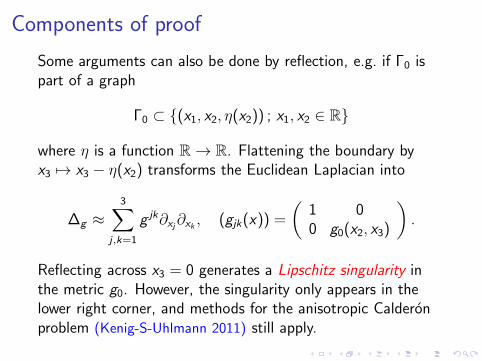
Some arguments can also be done by reflection, e.g. if Γ0 ispart of a graph

Γ0 ⊂ (x1, x2, η(x2)) ; x1, x2 ∈ R

where η is a function R → R. Flattening the boundary byx3 7→ x3 − η(x2) transforms the Euclidean Laplacian into

∆g ≈

3∑

j ,k=1

g jk∂xj∂xk , (gjk(x)) =

(1 00 g0(x2, x3)

)

.

Reflecting across x3 = 0 generates a Lipschitz singularity inthe metric g0. However, the singularity only appears in thelower right corner, and methods for the anisotropic Calderonproblem (Kenig-S-Uhlmann 2011) still apply.

Components of proof

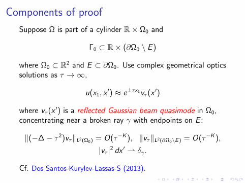
Suppose Ω is part of a cylinder R× Ω0 and

Γ0 ⊂ R× (∂Ω0 \ E )

where Ω0 ⊂ R2 and E ⊂ ∂Ω0. Use complex geometrical optics

solutions as τ → ∞,

u(x1, x′) ≈ e±τx1vτ (x

′)

where vτ (x′) is a reflected Gaussian beam quasimode in Ω0,

concentrating near a broken ray γ with endpoints on E :

‖(−∆− τ 2)vτ‖L2(Ω0) = O(τ−K), ‖vτ‖L2(∂Ω0\E) = O(τ−K ),

|vτ |2 dx ′ δγ .

Cf. Dos Santos-Kurylev-Lassas-S (2013).

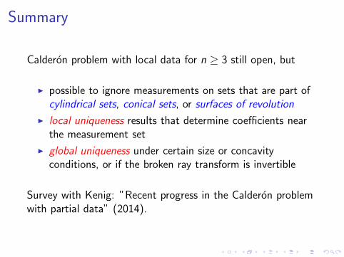
Summary

Calderon problem with local data for n ≥ 3 still open, but

possible to ignore measurements on sets that are part ofcylindrical sets, conical sets, or surfaces of revolution

local uniqueness results that determine coefficients nearthe measurement set

global uniqueness under certain size or concavityconditions, or if the broken ray transform is invertible

Survey with Kenig: ”Recent progress in the Calderon problemwith partial data” (2014).

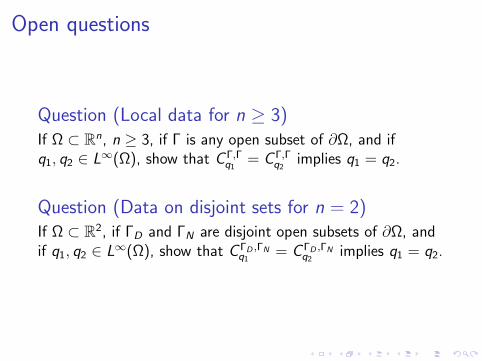
Open questions

Question (Local data for n ≥ 3)If Ω ⊂ Rn, n ≥ 3, if Γ is any open subset of ∂Ω, and ifq1, q2 ∈ L∞(Ω), show that C Γ,Γ

q1= C Γ,Γ

q2implies q1 = q2.

Question (Data on disjoint sets for n = 2)If Ω ⊂ R2, if ΓD and ΓN are disjoint open subsets of ∂Ω, andif q1, q2 ∈ L∞(Ω), show that C ΓD ,ΓN

q1= C ΓD ,ΓN

q2implies q1 = q2.