The ablative Hele-Shaw model for ICF flows - Inria · Plan Introduction Quasi-isobar model...

Hugues Egly,B. D. and R.

Sentis

The ablative Hele-Shaw model for ICF flows

Hugues Egly, B. D. and R. Sentis

April 2009

The ablative Hele-Shaw model for ICF flows p. 1 / 17

Plan

Introduction

Quasi-isobarmodel

Hele-Shawmodel :uvort = 0

The ablativeHele-Shawmodel

Conclusion

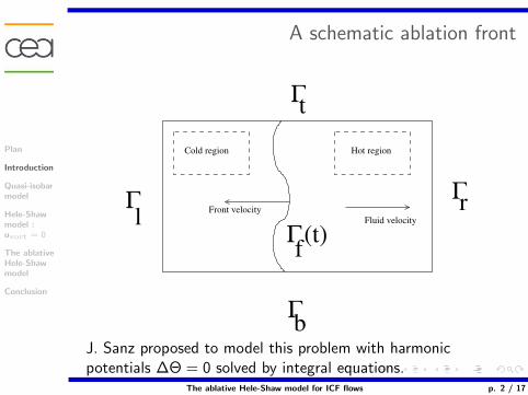
A schematic ablation front

Fluid velocityFront velocity

Cold region Hot region

Γ

Γ

Γ

Γb

r

t

lΓ (t)f

J. Sanz proposed to model this problem with harmonicpotentials ∆Θ = 0 solved by integral equations.


Plan

Introduction

Quasi-isobarmodel



Conclusion

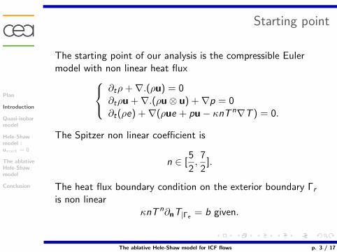
Starting point

The starting point of our analysis is the compressible Eulermodel with non linear heat flux

∂tρ +∇.(ρu) = 0∂tρu +∇.(ρu⊗ u) +∇p = 0∂t(ρe) +∇(ρue + pu− κnT n∇T ) = 0.

The Spitzer non linear coefficient is

n ∈ [5

2,7

2].

The heat flux boundary condition on the exterior boundary Γr

is non linearκnT n∂nT|Γe

= b given.


Plan

Introduction

Quasi-isobarmodel



Conclusion

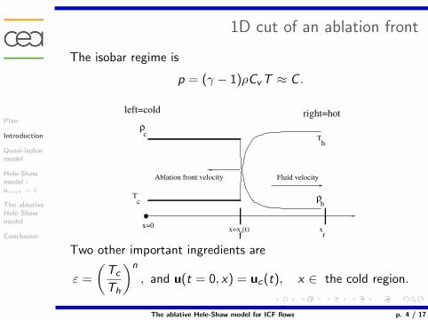
1D cut of an ablation front

The isobar regime is

p = (γ − 1)ρCvT ≈ C .

Fluid velocityAblation front velocity

x=0 x=x (t)f

xr

Tc

ρc

ρ

Th

h

left=cold right=hot

Two other important ingredients are

ε =

(Tc

Th

)n

, and u(t = 0, x) = uc(t), x ∈ the cold region.


Plan

Introduction

Quasi-isobarmodel



Conclusion

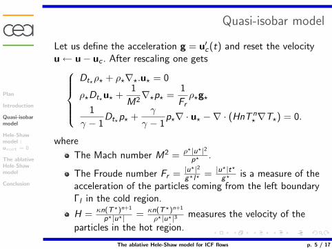
Quasi-isobar model

Let us define the acceleration g = u′c(t) and reset the velocityu← u− uc . After rescaling one gets

Dt?ρ? + ρ?∇?.u? = 0

ρ?Dt?u? +1

M2∇?p? =

1

Frρ?g?

1

γ − 1Dt?p? +

γ

γ − 1p?∇ · u? −∇ · (HnT n

?∇T?) = 0.

where

The Mach number M2 = ρ?|u?|2p? .

The Froude number Fr = |u?|2g?l? = |u?|t?

g? is a measure of theacceleration of the particles coming from the left boundaryΓl in the cold region.

H = κn(T?)n+1

p?|u?| = κn(T?)n+1

ρ?|u?|3 measures the velocity of the

particles in the hot region.


Plan

Introduction

Quasi-isobarmodel



Conclusion

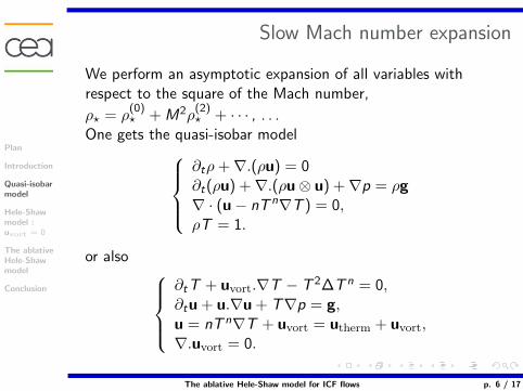
Slow Mach number expansion

We perform an asymptotic expansion of all variables withrespect to the square of the Mach number,

ρ? = ρ(0)? + M2ρ

(2)? + · · · , . . .

One gets the quasi-isobar model∂tρ +∇.(ρu) = 0∂t(ρu) +∇.(ρu⊗ u) +∇p = ρg∇ · (u− nT n∇T ) = 0,ρT = 1.

or also ∂tT + uvort.∇T − T 2∆T n = 0,∂tu + u.∇u + T∇p = g,u = nT n∇T + uvort = utherm + uvort,∇.uvort = 0.


Plan

Introduction

Quasi-isobarmodel



Conclusion

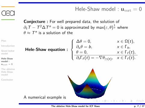
Hele-Shaw model : uvort = 0

Conjecture : For well prepared data, the solution of

∂tT − T 2∆T n = 0 is approximated by max(ε, θ)1n where

θ ≈ T n is a solution of the

Hele-Shaw equation :

∆θ = 0, x ∈ Ω(t),∂nθ = b, x ∈ Γh,θ = 0, x ∈ Γf (t),

∂tΓf (t) = −∇θ|γ(t), x ∈ Γf (t).

A numerical example is


Plan

Introduction

Quasi-isobarmodel



Conclusion

Main idea of the 1D proof

Set Θ = T n. Then ∂t

(1

Θ1n

)+ ∂xxΘ = 0. Progressive waves are

defined by Θ = Θ(x + vt). The generating Kull’s function isthe progressive wave with v = 1 and Θ(−∞) = 1

K ′(x) = 1− K− 1n (x), normalisation K (0) =

(n + 2

n + 1

)n

≈ e.

Set T =(εK

(x−x0+vt

ε

)) 1n . Then (T n)(−∞) = ε

1n ,

(T n)′(+∞) = v and ε1n ∂tT − T 2∂xxT

n = 0.

n(T )’=v

y

T

ε1/n

v


Plan

Introduction

Quasi-isobarmodel



Conclusion

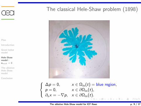
The classical Hele-Shaw problem (1898)

∆p = 0, x ∈ Ωin(t) = blue region,p = 0, x ∈ ∂Ωin(t),∂nx = −∇p, x ∈ ∂Ωin(t).


Plan

Introduction

Quasi-isobarmodel



Conclusion

Numerical result in 2D

We use a Finite Element Method for the Poisson equation, andmarkers for the front. The markers move accordingly to theHele-Shaw model.

0

0.2

0.4

0.6

0.8

1

0 0.2 0.4 0.6 0.8 1

t=0

t=0.06

Solution numeriqueSolution analytique

0.26

0.28

0.3

0.32

0.34

0.36

0.38

0.4

0.42

0 0.01 0.02 0.03 0.04 0.05 0.06

R(t

)

temps

solution numeriquesolution analytique

Grid 65*65 points. 65 markers are used to discretizeΓint(t) = Γf (t). On the left Γint(t). On the right t 7→ r(t).


Plan

Introduction

Quasi-isobarmodel



Conclusion

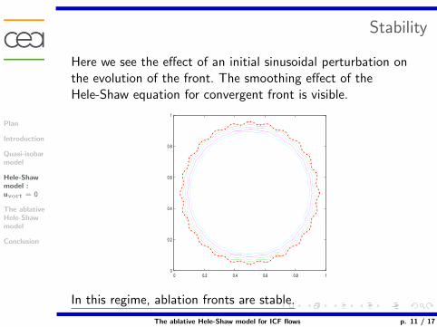
Stability

Here we see the effect of an initial sinusoidal perturbation onthe evolution of the front. The smoothing effect of theHele-Shaw equation for convergent front is visible.

0

0.2

0.4

0.6

0.8

1

0 0.2 0.4 0.6 0.8 1

In this regime, ablation fronts are stable.


Plan

Introduction

Quasi-isobarmodel



Conclusion

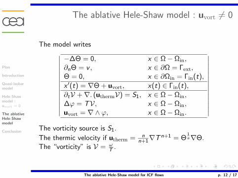
The ablative Hele-Shaw model : uvort 6= 0

The model writes∣∣∣∣∣∣∣∣∣∣∣∣∣∣

−∆Θ = 0, x ∈ Ω− Ωin,∂nΘ = v , x ∈ ∂Ω = Γext,Θ = 0, x ∈ ∂Ωin = Γin(t),

x ′(t) = ∇Θ + uvort, x(t) ∈ Γin(t),

∂tV +∇. (uthermV) = S1, x ∈ Ω− Ωin,∆ϕ = TV, x ∈ Ω− Ωin,uvort = ∇∧ ϕ, x ∈ Ω− Ωin.

∣∣∣∣∣∣∣∣∣∣∣∣∣∣The vorticity source is S1.

The thermic velocity if utherm = nn+1∇T n+1 = Θ

1n∇Θ.

The “vorticity” is V = ωT .


Plan

Introduction

Quasi-isobarmodel



Conclusion

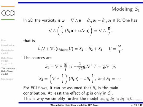
Modeling S1

In 2D the vorticity is ω = ∇∧ u = ∂x1u2 − ∂x2u1 ∈ R. One has

∇∧(

1

T(∂tu + u.∇u)

)= ∇∧ g

T,

that is

∂tV +∇. (uthermV) = S1 + S2 + S3, V =ω

T.

The sources are

S1 = ∇∧ g

T≈ − 1

T 2g.∇⊥T = g.∇⊥ρ,

S2 =

(∇∧ 1

T

)(∂tu)− ω∂t

1

T, and S3 = · · ·

For FCI flows, it can be assumed that S1 is the maincontribution. At least the effect of g is only in S1.This is why we simplify further the model using S2 ≈ S3 ≈ 0.


Plan

Introduction

Quasi-isobarmodel



Conclusion

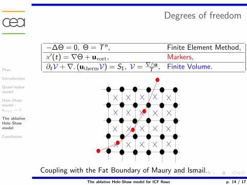
Degrees of freedom

∣∣∣∣∣∣−∆Θ = 0, Θ = T n, Finite Element Method,

x ′(t) = ∇Θ + uvort, Markers,

∂tV +∇. (uthermV) = S1, V = ∇∧uT , Finite Volume.

∣∣∣∣∣∣

Coupling with the Fat Boundary of Maury and Ismail.


Plan

Introduction

Quasi-isobarmodel



Conclusion

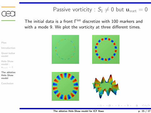
Passive vorticity : S1 6= 0 but uvort = 0

The initial data is a front Γint discretize with 100 markers andwith a mode 9. We plot the vorticity at three different times.


Plan

Introduction

Quasi-isobarmodel



Conclusion

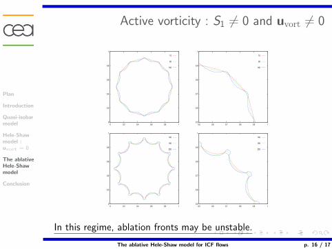
Active vorticity : S1 6= 0 and uvort 6= 0

0

0.2

0.4

0.6

0.8

1

0 0.2 0.4 0.6 0.8 1

10

80

140

0.5

0.6

0.7

0.8

0.9

1

0.5 0.6 0.7 0.8 0.9 1

10

80

140

0

0.2

0.4

0.6

0.8

1

0 0.2 0.4 0.6 0.8 1

140

180

220

0.5

0.6

0.7

0.8

0.9

1

0.5 0.6 0.7 0.8 0.9 1

140

180

220

In this regime, ablation fronts may be unstable.


Plan

Introduction

Quasi-isobarmodel



Conclusion

Conclusion

• We have derived the ablative Hele-Shaw model for ICF flows∣∣∣∣∣∣∣∣∣∣∣∣∣∣

−∆Θ = 0, x ∈ Ωext(t) = Ω− Ωin(t),∂nΘ = v , x ∈ ∂Ω = Γext,Θ = 0, x ∈ ∂Ωin(t) = Γin(t),

x ′(t) = ∇Θ + uvort, x(t) ∈ Γin(t).

∂tV +∇. (uthermV) = ∇∧ gT , x ∈ Ω− Ωin,

∆ϕ = TV, x ∈ Ω− Ωin,uvort = ∇∧ ϕ, x ∈ Ω− Ωin.

∣∣∣∣∣∣∣∣∣∣∣∣∣∣• Plenty of open problems.• See H. Egly PhD thesis for more numerical results.• Cf the Web page of Howison (Ociam, Oxford) for somehistorical references about Hele-Shaw (and also with freshscience) : “Mr Hele-Shaw (inv. of the variable pitch propeller)worked on the propeller of the cruisers of her gracious majesty”.


The ablative Hele-Shaw model for ICF flows - Inria · Plan Introduction Quasi-isobar model...

Documents

Transcript of The ablative Hele-Shaw model for ICF flows - Inria · Plan Introduction Quasi-isobar model...