Testing the Responses of Three PSF Fitting Methods

Meridith Joyce

John Marriner

Fermilab

August 10, 2012

ABSTRACT

We present an analysis of prototype code designed to fit point-spread functions to

point-like astronomical objects appearing in images taken by DECam, or the Dark

Energy Camera. We test three methods, each of which yields a maximum likelihood

estimate for a different likelihood function. We call these methods Poisson likelihood,

χ2 with background error, and χ2 with data error, and describe their differences mathe-

matically. Each is used to construct a fit involving up to four parameters characterizing

the raw pixel data. We measure biases in the signal and background levels under a

variety of conditions. We test the variance and error estimate of the fits as a function

of signal strength, outline areas of sensitivity, and demonstrate the effects of incomplete

or inaccurate information on the Poisson fit. We conclude that the Poisson likelihood

fitting method is best, as it is successful in all circumstances under which the χ2 series

are, and displays other favorable attributes where the others do not.

1. Introduction

One of the most important astronomical measurements is a precise determination of the flux of

a distant object. Because observations have significant measurement errors, parameter estimation

techniques are used to obtain measurements of the flux. One of the applications of photometry is

to provide the best estimator of the brightness of astronomical objects that can be determined from

images of the sky. One approach to this problem is aperture photometry, in which the brightness

of an object is measured by counting photons in a given region of an image after performing

background-subtraction. This method is robust because it is insensitive to the shape of the object

or its position. However, it is more sensitive to statistical errors. For bright objects, this method

is effective, but it is weak statistically, or inefficient, and therefore less precise for faint objects.

Another method is PSF photometry. The ”point-spread function,” or PSF, describes the response

of an imaging system when measuring point-like objects. On a digitized image, a point-like object is

observed as an array of pixels that forms a 2-dimensional peak around the center of the source; e.g.

the point of light is ”smeared out,” or spread statistically, over a larger region. When we investigate

faint stars, which are effectively point sources, the more efficient PSF photometry is preferable, but

– 2 –

requires attention to the shape and location of the center, which can introduce errors. If the star

is faint, the position is uncertain and the estimate for the flux will be biased. We expect a bias in

flux when the position is fit because the displacement from the center can only be positive, since

it is measured radially. We develop computer code that simulates observations and uses variations

on a mathematical function known as the ”likelihood function” (see §2) used to estimate up to four

parameters characterizing data. We analyze the precision and bias of the program when applied

to simulated data. We derive the mathematical techniques and test three fitting methods: Poisson

likelihood, chi-squared with background error, and chi-squared with data error, in four parameter

systems. We describe the numerical methods used in constructing the fits in section 2 and present

graphical comparisons of the methods in sections 4 and 5. We demonstrate where biases and other

errors occur and comment on the effectiveness of each method under various parameter systems and

fitting options. We conclude that the Poisson likelihood fitting method is accurate in the largest

range of conditions and produces a bias consistent with zero in all cases where there is sufficient

signal level.

2. Numerical Methods

We describe the mathematics behind the PSF and our fitting methods.

In an image, we assume an observation of a grid of N×N pixels, where the pixels are numbered

from 1 toN2 and the ith pixel observation is ni photoelectrons. The ni are not integer values because

of readout noise, and each observation is equal to the average number of photons n̄i plus statistical

fluctuations. We further assume that there is a point-spread function (PSF) that describes the

distribution of light from a point source that is known with negligible error and is given by the

function P(x,y). We model the average number of photo-electrons by

n̄i = AP (xi − sx, yi − sy) +B (1)

where A is the amplitude of the source (amount of signal), B is the level of background counts,

and sx and sy give the centering of the PSF.

We can estimate the parameters A, B, sx, and sy by finding the values that maximize a

likelihood function. We consider two possible approximations to the likelihood function. The first

form assumes that the ni follow a chi-squared distribution with error σi (which is approximately

true when the ni are large). The likelihood is

L = e(−χ2/2) (2)

−2 ln(L) = χ2 (3)

=N2∑i=1

[ n̄iσi

]2. (4)

– 3 –

We implement two fitting techniques based on maximizing this form, and we refer to them as

”χ2 with data error” (shortened to ”χ2 data” in figures) and ”χ2 with background error” (shortened

to ”χ2 bkg” in figures) henceforth. The difference between them emerges with selection of the error

term σi. One obvious possibility is to approximate σi =√ni, but σi is not the true error because

of statistical fluctuations in the data. This is the χ2 data approach. Another common technique

is to set the σi to be some constant, say σi = B. This is the χ2 background approach. This latter

choice is not a very good estimate of the actual errors, but the maximum likelihood is insensitive to

the values of the σi and the technique works quite well. A more accurate method would be to set

σi =√n̄i, but this has the technical disadvantage of placing the fit parameters in the denominator

of the function being minimized, making the fit non-linear. However, if we fit for the PSF shift

parameters sx and sy, the fit is non-linear anyway, so the disadvantage is slight.

Instead of pursuing the option of σi =√n̄i, we examine a new approach that should be more

general. This alternative form is based on Poisson statistics.

L =

N2∏i=1|

e−n̄in̄ini!

(5)

ln(L) =N2∑i=1

−n̄i + ln n̄i − ni lnni + ni (6)

where we have used Stirling’s approximation

lnn! ≈ n lnn− n (7)

. We name the technique based on maximizing this variant ”Poisson likelihood,” and refer to it as

such subsequently. It can be shown that the Poisson likelihood is equivalent to setting σi =√n̄i in

Equation 4, when n̄i is large. A disadvantage of the Poisson likelihood method is that the non-linear

fit for parameters A and B requires iterative techniques, even when sx and sy are not being fit.

In general, the background will be smooth and the value of B can be estimated from pixels

outside the N × N grid. We can express this information as a prior on B in either the case of

Equation 4 or Equation 6 by adding an additional term

−2 ln(L′) = −2 ln(L) +(B −BP )2

σ2B

(8)

where BP represents the prior knowledge of B and σB the uncertainty.

3. Implementation

We choose to simulate a 25x25 pixel grid of observations. For most of our tests, the simulated

point source is centered on the grid, but we consider situations in which it is not, so the fit can adjust

– 4 –

for this in these cases by varying parameters sx and sy. We construct a PSF on a similar 51x51 grid,

and the PSF is shifted by sx and sy using Lanczos interpolation in the process of fitting for sx and

sy. The PSF is shifted, scaled, and interpolated to match the data. We implement routines that

construct a series of simulated observations based on point-like objects using the PSF, but with

added errors due to photon statistics and readnoise. We compare the numbers generated by these

functions to ”true value” parameters A, B, sx and sy which were used to generate the simulated

observations. Our nominal values correspond approximately to DECam exposures of 100 seconds

in the g-band, and are given by A = 1062, B = 742, sx = 0 and sy = 0. These numbers roughly

translate to expecting a detectable signal, moderate background noise, and known centering of the

PSF. We use a set of control variables to manipulate the conditions and type of fit. We track

the discrepancy between the ”true fit,” a preexisting correct answer determined by which values

are selected for A,B, sx and sy, and the fit generated by the computer. Reasons for discrepancies

between them include low signal, high background noise, and incorrectly centering the PSF.

We run all simulations in one of four possible parameter systems. We use the variable n to

denote which set of parameters is being fit. The first case, denoted by n = 1, involves fitting only

for A (signal only), the second, n = 2, fits for A and B (signal and background), the third, n = 3,

fits for A, sx and sy (signal and position), and the fourth, n = 4, fits for A, B, sx and sy (signal,

background, and position). If a parameter is not being fit, it is held at its fixed true value, which

for B is 742 and for sx and sy is 0. Every parameter system involves A, so it is never automatically

forced to a default value. Additionally, we experiment with forced errors and dependence on prior

information.

In the main program, a series of arrays is filled with statistical quantities describing a routine’s

computation. Routines written elsewhere are called to construct data and a Gaussian fit (PSF)

to that data from the values assigned to A, etc. by the user at onset. Choosing a fitting method

corresponds to choosing the way in which the computer will attempt to minimize the difference

between the data it generates and the fit it constructs. Two of the options for the fitting method, χ2

background and χ2 data, are based on the likelihood maximization function described in equation

(4). The other, Poisson likelihood, is described in equations (5) and (6) . The method we call

”χ2 data” is a χ2 minimization routine that takes into account error in the generated data; χ2

background is another minimization routine, but takes into account error in the signal background

instead. We are interested in assessing the comparative accuracy of these three methods, and do

so in the Comparison of Methods section. There we also highlight the advantages of the Poisson-

likelihood method.

The majority of data is presented as a function of the signal level, parameter A. We collect

biases, RMS values, and mean error estimates by calculating fits over a range of A values. We do

this by looping over a list of regularly-incremented values and assigning each one, in turn, to A,

and generating a new set of fit statistics for each outcome. If we are interested in the fit output for

various levels of background noise, we will increment B, and so forth. For a given set of fits, the

parameter NTRIALS controls the computational accuracy of the fit, which is the number of trials

– 5 –

run for a given set of fitting conditions. In other words, it is the number of trials used in computing

a single data point on the figures that follow. ”Trial” here is a statistical term, meaning a single set

of pseudo-randomly generated numbers, extracted from either a Poisson or Gaussian curve centered

at the true parameter value, used in computing the fit. NTRIALS is set to either 1000 or 10,000 for

all data shown below, meaning that at least 1000 statistical trials were computed per data point.

A set of fit values for A through sx, as well as biases, errors, RMS values, and other statistical

information, is collected for each trial, averaged over the number of trials, and these averages are

taken to be the best estimate of the fit information given a particular set of parameters. Using

multiple computations based on numbers near the intended values, taken from a distribution of

our selection and weighted by the likelihood of their occurrence, gives statistical robustness to the

outcome and serves to better simulate true astronomical data, which can be distorted by a plethora

of environmental and technological factors. It is important to note the difference between NTRIALS

and the statistic we call ”ntrials,” which is a measure of the number of attempted fits that succeed

for a given run. It is possible that a fit to the data will fail to converge, and if this happens, it is

a failed trial. The ratio ntrials:NTRIALS gives the percentage of trials that were successful. All

of the data shown below was computed under conditions that produced a 95% or better success

rate. The second fit-manipulating parameter, which we call ”sigma” (denoted as σP inEquation8,

dictates whether or not prior knowledge, e.g. a pr-existing input, is used in fitting for parameter

B. The σp value is a way of controlling the level of fluctuation from a known input permitted to

occur. A small, positive σp value requires the program to fit B with very little fluctuation from the

true value of B. A large, positive σp value lowers the impact prior knowledge of B has on the fit,

and a negative σp value dictates that no prior knowledge of B be used in fitting B.

4. Comparison of Methods

We compare the three fitting methods through an analysis of the bias, variance, and error

estimate for each of the parameter systems. We show the variance and bias in A as a function of A

for each fitting method for the 1, 2, 3, and 4-parameter cases. Additionally, we present plots of the

RMS and error estimates against A for all methods. Deeper analysis of the Poisson case, such as

its behavior in a small signal region, is given. NTRIALS values for subsequent figures range from

1000 to 10,000, and a σp of either 0.1 or -1 (heavy or no prior on B, respectively) is given where

relevant, i.e. for the 2- and 4-parameter systems. The initial value of B is supplied by the calling

program and is normally set to the true value of B = 742. NTRIALS and σp are invariant for the

data sets on each figure.

– 6 –

4.1. Bias

The bias is defined in our program as the true value of a parameter subtracted from the fit’s

calculation of that parameter; e.g. we define the bias in A as

fit.A−A (9)

where ”fit.A” is the element of the array containing the computed value of A. Biases will depend

on which parameters are being fit and which values have priors on them or not. We cover several

combinations.

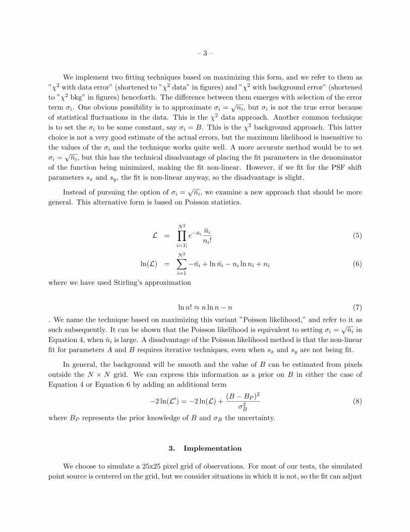
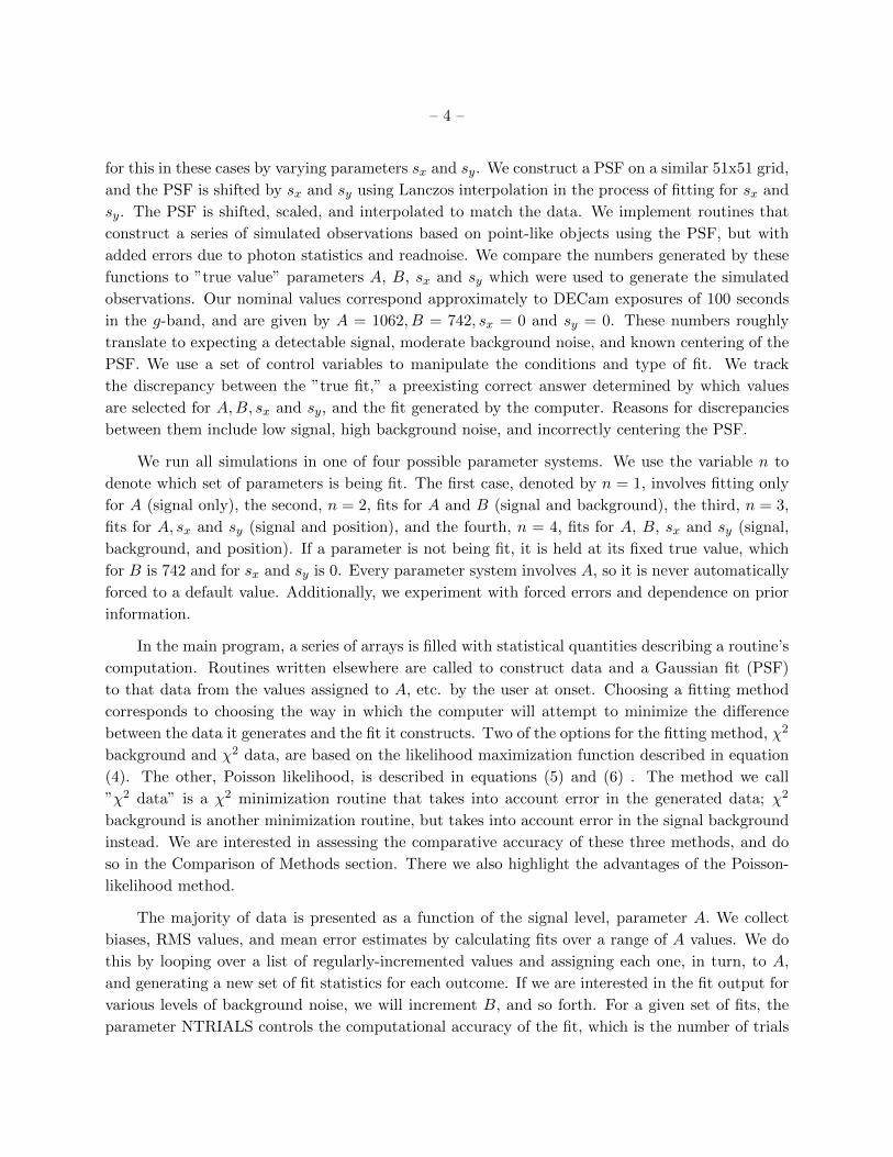
Bias in A as a function of A is plotted in Figures 1 and 2. Figure 1a depicts the parameter

system that fits for A, and Figure 1b shows the system that fits for both A and B. Figures 2a

and 2b show the fits for the system including A, sx, and sy, and the system including all four

parameters, respectively. Each grid shows the three fitting methods: Poisson likelihood as the

dotted series, χ2 with data error as triangles, and χ2 with background error as asterisks. The χ2 fit

with data error shows a large bias in the 1, and 3- parameter systems. The χ2 data fit may show

a slight positive bias in the 2-parameter case, but the bias is significantly smaller in magnitude in

the 2 and 4 parameter cases than in the 1 or 3 parameter cases. In all but the n = 1 and n = 3

cases, the bias in the χ2 data fit worsens as A increases. We observe that in all cases, the Poisson

likelihood and χ2 fit with background error are consistent with zero bias.

The difference in the severity of the biasing of the χ2 data fit between the 1 and 3 versus 2

and 4- parameter systems is due to the fact that the even-numbered parameter systems fit for B

and the others do not. Clearly the χ2 data fit is inherently biased, but fitting for B decreases the

negative effect.

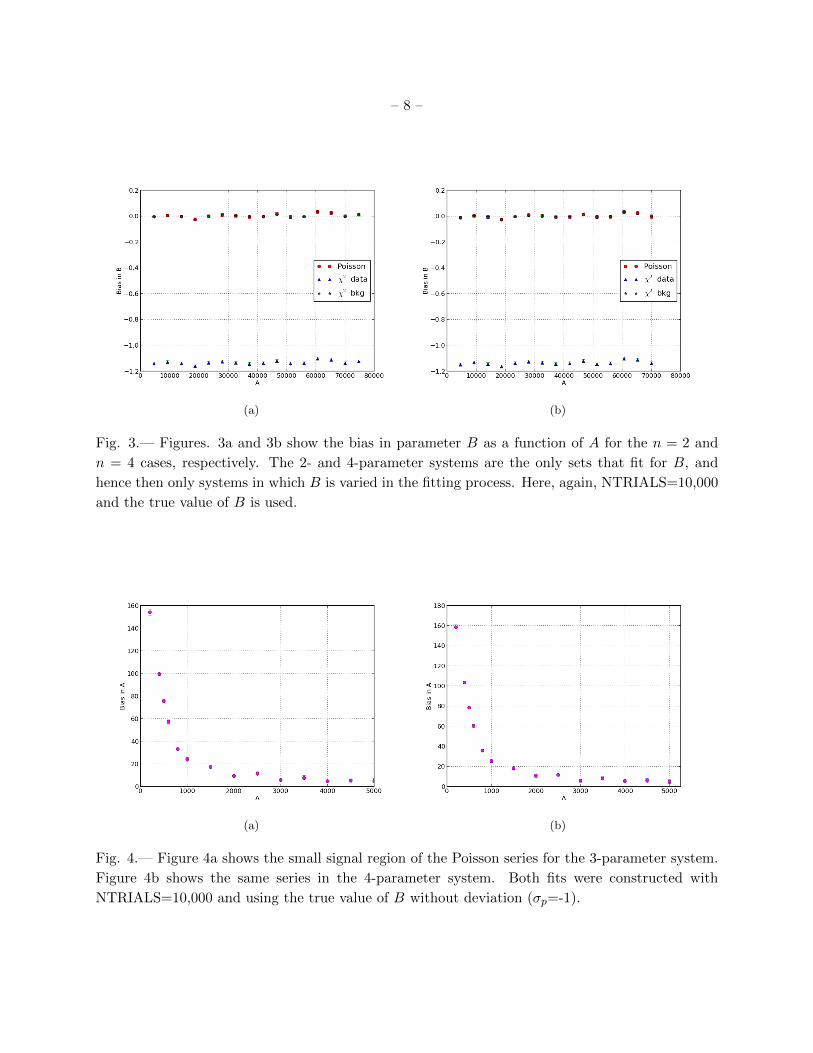
We measure the bias in B as a function of A for the 2- and 4-parameter systems (as these are

the only systems in which a fit for B is calculated). Figure 3a shows the three fits for n = 2, and

Figure 3b for n = 4. In both systems, the Poisson and χ2 background error fits are consistent with

zero bias in B. The χ2 data error fit shows a negative bias in both cases.

At A = 0, we expect the majority of the fitting trials to fail when the centering of the PSF is

being computed (sx and sy are being fit), as there is no signal from which to determine the center

of the PSF. For this reason, we do not include data at zero for any of the fits or systems, though a

fit could be computed in any parameter systems where sx and sy are not being fit. In Figure 4, we

show the Poisson likelihood fit in the small signal regions for the 3 and 4-parameter systems with

denser sampling over the 0-5000 range. We find that as signal strength increases, the bias decays

toward zero. All methods show similarly increasing bias decreasing signal strength The biasing in

low-signal regions is anticipated because it is harder to fit for position with small signal, and the

position error is always positive because it is measured radially.

Figure 5 shows another measure of the biases in parameters A and B, this time as a function

background prior, BP . Recall that the purpose of BP is to force an estimate of the background

– 7 –

(a) (b)

Fig. 1.— Figure 1a shows the bias in A of the 1-parameter model, which fits only for A, as a

function of A. Figure 1b shows the bias in A as a function of A in the 2-parameter model, which

fits for both A and B.

(a) (b)

Fig. 2.— Figure 2a shows the bias in A as a function of A for the 3-parameter model, which fits

for A, sx, and sy. Figure 2b shows the same, for the 4-parameter model, which encompasses fits

for A, B, sx, and sy. The series are labeled as above.

– 8 –

(a) (b)

Fig. 3.— Figures. 3a and 3b show the bias in parameter B as a function of A for the n = 2 and

n = 4 cases, respectively. The 2- and 4-parameter systems are the only sets that fit for B, and

hence then only systems in which B is varied in the fitting process. Here, again, NTRIALS=10,000

and the true value of B is used.

(a) (b)

Fig. 4.— Figure 4a shows the small signal region of the Poisson series for the 3-parameter system.

Figure 4b shows the same series in the 4-parameter system. Both fits were constructed with

NTRIALS=10,000 and using the true value of B without deviation (σp=-1).

– 9 –

level (parameter B) in calculating the fit (refer to equation 8). In these plots, we set A and B to

their true values (1062 and 742, respectively) and investigate how the bias in fitting these varies

over a range of background estimates. The graphs indicate that as BP approaches the true value

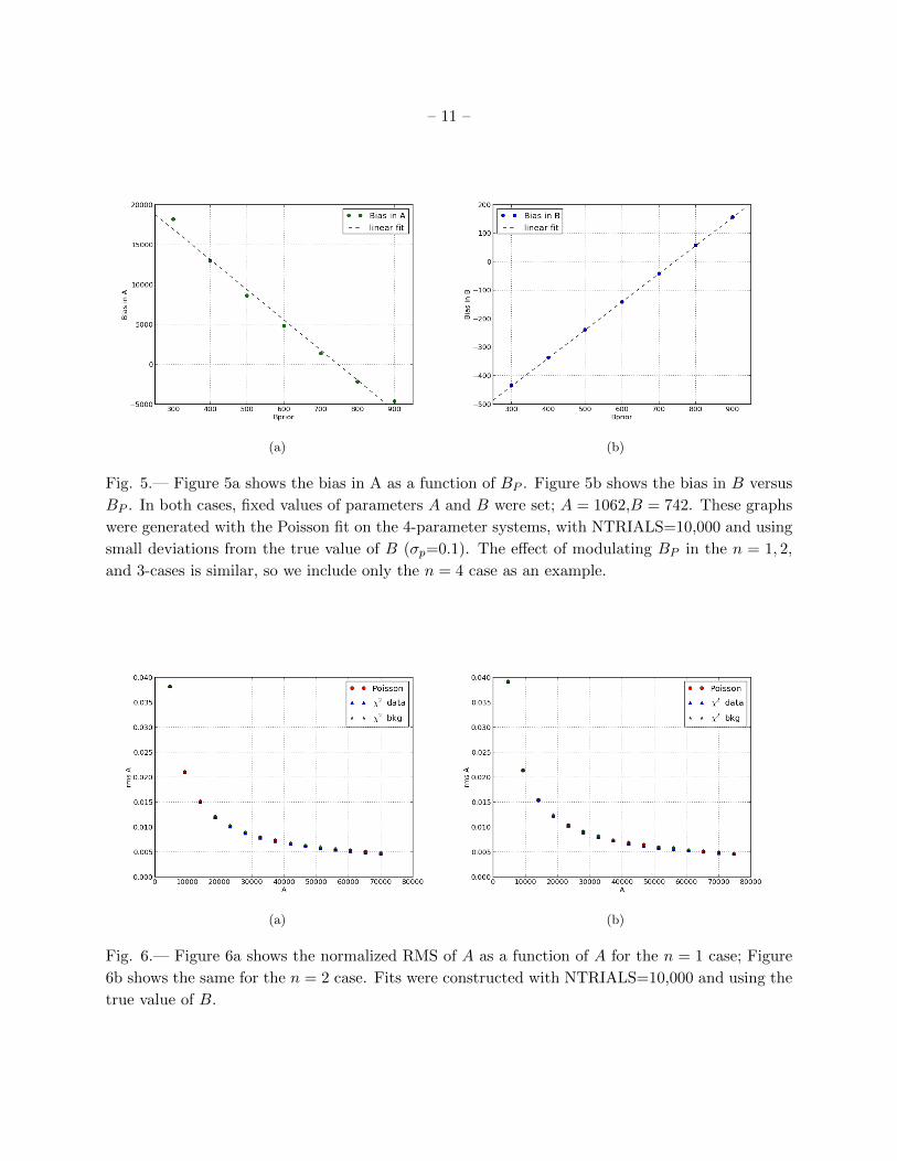
of B, the biases in both A and B approach zero. For both 5a and 5b we provide linear fits of the

bias curves. In 5a, we note that the curve displays non-linear features, but for the small range we

are considering, a linear approximation suffices. The function describing the linear fit is given by

f(x) = −37.8x+ 28246 (10)

. The important feature of this equation is the slope, which describes the ratio of error between BPand A. With magnitude of approximately 1:40, we determine that an error of 0.1 in BP corresponds

to an error of approximately 4 in A. Understanding this effect enables a correction formula to be

used, if the error in BP is known or can be estimated.

In Figure 5b, the linear fit is given by

f(x) = 0.986x− 731.3, (11)

and we are again primarily concerned with the slope. We expect the slope to be unity, as forcing a

prior on B intrinsically changes the value computed for B, since the computer must use the prior.

The difference between whatever value is used for BP and the true value of B will be exactly the

bias in B. We conclude that the biases in both A and B depend on BP and vanishl as the true

background level is approached.

4.2. Variance

The variance of a parameter is an indication of the amount of fluctuation between trials, or

”spread” of the data. The variance in A is defined mathematically as the RMS value for each data

point. The RMS is given by √Σ

x2i

ntrial− x̄2, (12)

where xi represents once instance of the bias, or difference between the true value of a parameter and

its computed value, x̄ represents the average value of the bias, and ntrial is the number of successful

fits. Figure 6 shows the variance in A divided by A, or normalized variance, as a function of A for

the n = 1 and n = 2 cases, and Figure 7 shows the same for the n = 3 and n = 4 cases. While

the variance curves are nearly identical for all fits and parameter systems, plotting a subtracted

curve reveals a difference between the fits. While the differences are statistically significant, they

are negligible, occurring on a scale 3 orders of magnitude smaller than scale on which the curves

are presented.

A peak value ranging between 0.35 and 0.40 occurs at the first sampled point for each fit in each

parameter system, whereafter the variance decays with increased signal strength. Less fluctuation

– 10 –

with improved signal strength is anticipated, though the variance decays much more slowly than

the bias.

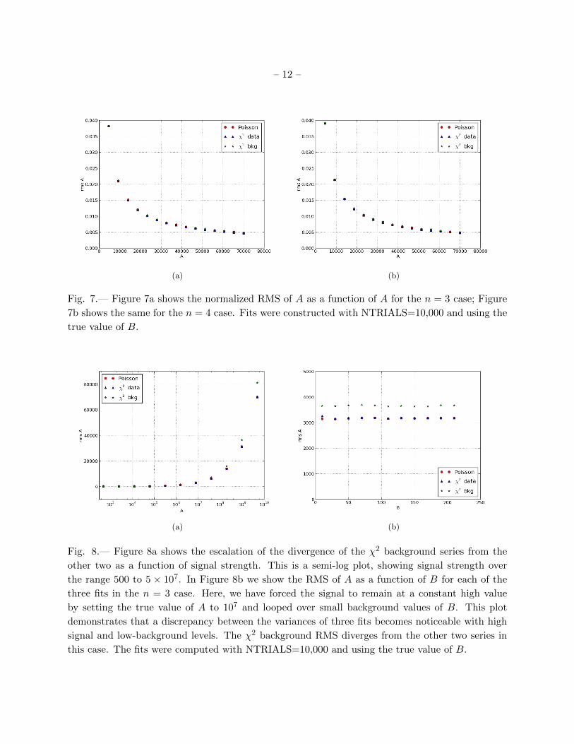
Figures 8a and 8b provide additional details on the fits. Figure 8a highlights the divergence

of the χ2 background series from the Poisson likelihood and χ2 data series as signal strength is

increased to very high values. This plot is logarithmic in the x-axis, and shows the behavior of all

three fits for the n = 3 case for signal strengths up to A = 5× 107. In Figure 8a, the background

level is set at B = 742. In Figure 8b, we examine a region with high signal strength (A = 107)

and low bias, which serves to contrast the previous scenarios, in which the signal-to-bias ratio was

much lower. If we compare this RMS plot to the one constructed for the n = 3 case in Figure 7, we

see that the high signal case does not show a decay and displays a discrepancy between the three

fitting methods, most noticeably in the χ2 background series. In the typical signal range used in

earlier figures, we see that the RMSs of the three fits align nearly identically, and decay toward

zero. We note that in this case (figures 8(a) and 8(b)), the true value of B was set to 742. In

the high signal series, the RMS is much larger, meaning there is a much higher variance among

the data points, and that the fits behave distinctly. The Poisson and χ2 with data error series do

not align to within minute discrepancy, as is the case in the normal signal range, and the χ2 with

background error series demonstrates a much higher variance over the given range of background

levels. In figures 6 and 7, we varied A and kept B at its true value, whereas in Figure 8b, the

background level is varied over a range of small values, and the signal is high. Despite the different

plotting schemes, it is easy to see that the fits behave differently in the two situations. We see that

the χ2 fit with background error behaves most unfavorably of the three under these conditions,

and that the Poisson fit works just as well as, but not significantly better than, the traditional χ2

fitting method with data error.

4.3. Error Estimate

In addition, we collected measurements of the error estimate of each fit as a function of A.

The fit estimates parameter errors based on the input image data. More generally, each parameter

in the likelihood or minimization routine has an associated uncertainty. The error estimate is

calculated by summing the square of the fit error on each parameter for each iteration, dividing by

the number of successful fits (ntrials), and taking the square root of that value. The error estimate

is based on the errors of each input to the fitting routines; it is not related to the true values.

The square of the error associated with each of A, B, sx, and sy is recorded along the diagonal

of a covariance matrix. The total error of the fit is calculated from the errors on each relevant

constituent in the matrix (A and B for n = 2, and so forth). This value is recorded for each data

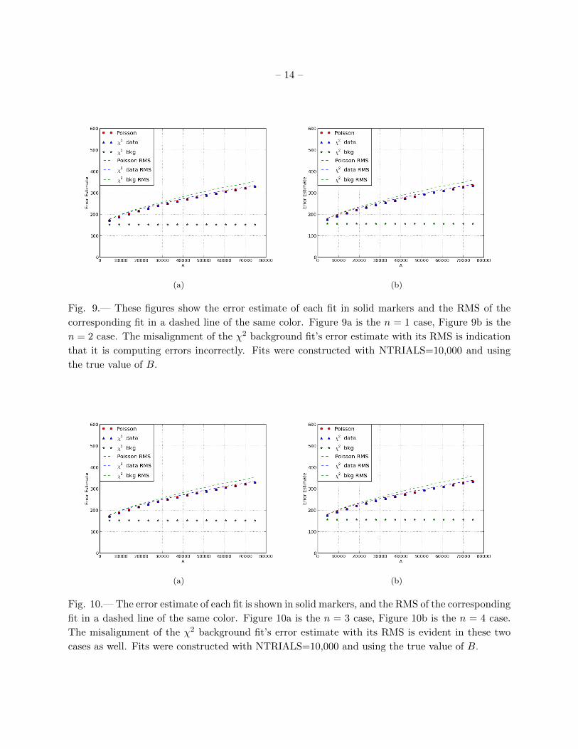
point. Figures 9 (n = 1, 2 cases) and 10 (n = 3, 4 cases) show the error estimate versus A for

each parameter system. The most noticeable observation is the constancy of the χ2 background

series in all four cases. While the error estimates in the Poisson and data error series increase with

signal strength, the background error series remains fixed at an error estimate lower than is ever

– 11 –

(a) (b)

Fig. 5.— Figure 5a shows the bias in A as a function of BP . Figure 5b shows the bias in B versus

BP . In both cases, fixed values of parameters A and B were set; A = 1062,B = 742. These graphs

were generated with the Poisson fit on the 4-parameter systems, with NTRIALS=10,000 and using

small deviations from the true value of B (σp=0.1). The effect of modulating BP in the n = 1, 2,

and 3-cases is similar, so we include only the n = 4 case as an example.

(a) (b)

Fig. 6.— Figure 6a shows the normalized RMS of A as a function of A for the n = 1 case; Figure

6b shows the same for the n = 2 case. Fits were constructed with NTRIALS=10,000 and using the

true value of B.

– 12 –

(a) (b)

Fig. 7.— Figure 7a shows the normalized RMS of A as a function of A for the n = 3 case; Figure

7b shows the same for the n = 4 case. Fits were constructed with NTRIALS=10,000 and using the

true value of B.

(a) (b)

Fig. 8.— Figure 8a shows the escalation of the divergence of the χ2 background series from the

other two as a function of signal strength. This is a semi-log plot, showing signal strength over

the range 500 to 5 × 107. In Figure 8b we show the RMS of A as a function of B for each of the

three fits in the n = 3 case. Here, we have forced the signal to remain at a constant high value

by setting the true value of A to 107 and looped over small background values of B. This plot

demonstrates that a discrepancy between the variances of three fits becomes noticeable with high

signal and low-background levels. The χ2 background RMS diverges from the other two series in

this case. The fits were computed with NTRIALS=10,000 and using the true value of B.

– 13 –

reached by either of the other series because the error in the χ2 background series does not depend

on signal strength. The explanation for this behavior is that the χ2 background fit estimates the

error values incorrectly, except when A = 0, highlighting an obvious problem in this choice of fit.

This explanation is substantiated by the series that show the RMS, without normalization by A,

as dashed curves next to the error estimate series for each fit. In all of these figures, we see that

the RMS of the χ2 background series follows a curve very similar to those of the Poisson and χ2

data fits, whereas the actual error estimate is low and does not display any curvature. This shows

that the χ2 background series does not compute the error correctly. If it did, its error estimate and

RMS would be nearly the same, as they are in the case of the other two fits. The χ2 background fit

computes the error incorrectly because the fit uses a background estimate σi (see §2), which results

in a flat error estimate despite increased signal. The error estimate should increase with increased

signal, a behavior that the Poisson and χ2 data fits both demonstrate.

4.4. Discussion

The standard statistical indicators examined here – bias, variance, and error estimate – show

that the fit based on Poisson statistics is a superior method to either of the χ2 fits. In measures

of bias, the Poisson fit yields biases consistent with zero for both A and B as a function of signal

strength when sx and sy are fit. This is not true of the χ2 data method. In measures of variance, all

three fits behave similarly, with the exception of the high signal range, in which the χ2 background

fit diverges and shows a higher variance than the other two. In measures of the error estimate,

the χ2 background fit fails to fit the errors, and hence does not provide any reliable measure. The

Poisson and χ2 data fits show the same behavior. From these graphical analyses, we glean that

the fit based on Poisson statistics is more efficient and reliable, as it succeeds in every one of these

statistical categories, unlike either of the χ2 methods. We conclude that the Poisson method is

best for fitting the PSF.

5. Sensitivity to Data and Error Model

Having analyzed the Poisson fitting method under typical conditions alongside that of the χ2

methods and concluded that it is the best fitting routine, we include more detailed analysis of the

Poisson likelihood fitting method and highlight its sensitivities. We concentrate on the behavior of

the Poisson likelihood method, but note that the other methods should behave similarly.

5.1. Sensitivity to PSF

Figure 11 maps the behavior of the Poisson fit with the true value of A held at its standard

value of 1062. but with the true value of B set to a series of values incremented over multiplication

– 14 –

(a) (b)

Fig. 9.— These figures show the error estimate of each fit in solid markers and the RMS of the

corresponding fit in a dashed line of the same color. Figure 9a is the n = 1 case, Figure 9b is the

n = 2 case. The misalignment of the χ2 background fit’s error estimate with its RMS is indication

that it is computing errors incorrectly. Fits were constructed with NTRIALS=10,000 and using

the true value of B.

(a) (b)

Fig. 10.— The error estimate of each fit is shown in solid markers, and the RMS of the corresponding

fit in a dashed line of the same color. Figure 10a is the n = 3 case, Figure 10b is the n = 4 case.

The misalignment of the χ2 background fit’s error estimate with its RMS is evident in these two

cases as well. Fits were constructed with NTRIALS=10,000 and using the true value of B.

– 15 –

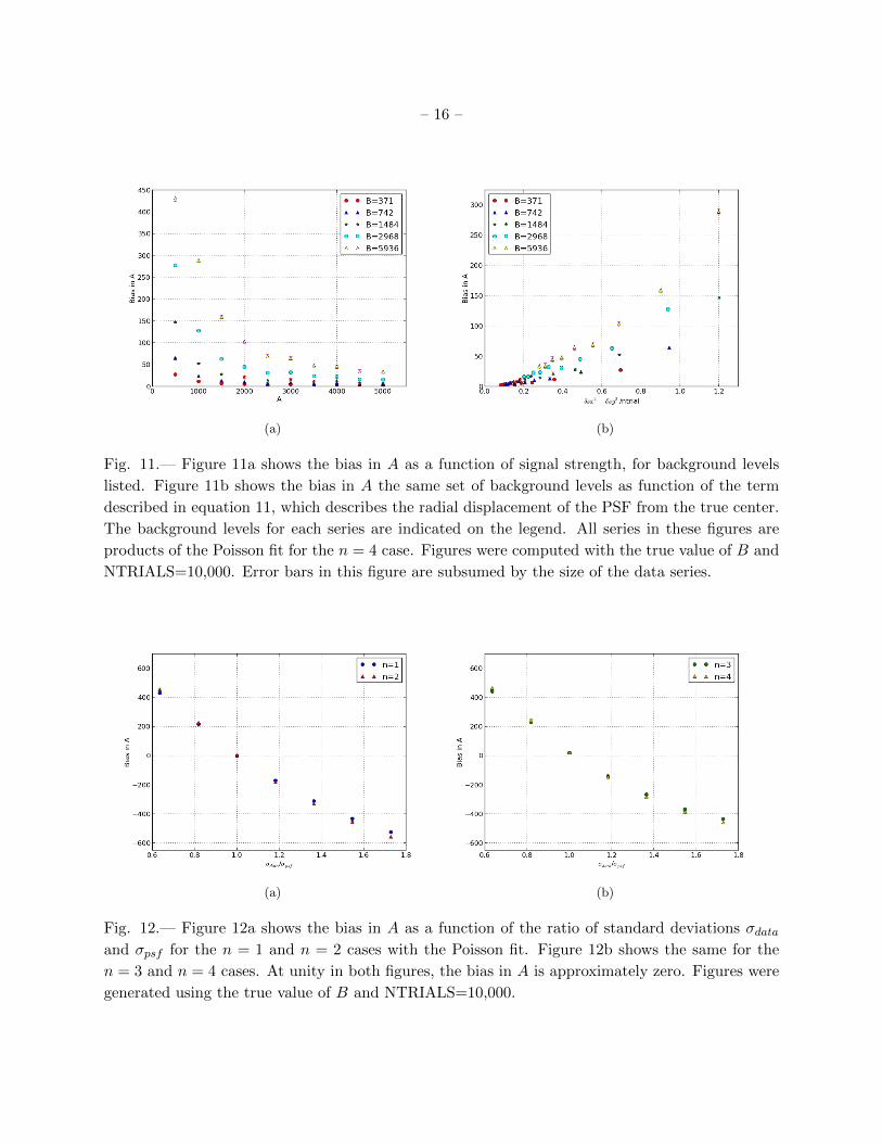
by two, beginning with B = 371 and extended to B = 5936. We plot the bias in A for each of these

B values as a function of the term

δsx2 + δsy2

ntrial, (13)

which is a composition of three variables that are tracked in the construction of the fit: ntrial,

which logs the number of fits that succeed, and δsx and δsy, which are the error estimates of the

position. Note that displacement can only be positive, since the center is taken at sx = sy = 0.

Figure 11a shows the bias in A as a function of signal strength for a series of B background

levels ranging from half of the true B value to 8× the true B value. This is shown in the small

signal region A = 500 to A = 5000. We see negative effects here for the higher B levels, and

note that although the series decay for every B value, the bias is larger when B is large. Figure

11b indicates that as the radial error estimate increases from zero, the bias in A increases rapidly.

Because an error in centering the PSF will affect the bias, the dependence on the error estimate is

expected. The figure also demonstrates that with higher background level, the bias is stronger and

increases more rapidly.

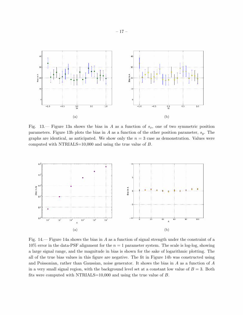
Two more behaviors we investigate for the Poisson likelihood fit are shown in Figure 14. The

first, Figure 14a, is relevant to measures of sensitivity to the PSF. The bias’s response to a 10%

misalignment error between the standard deviation of the data curve and the standard deviation

of the PSF is shown in Figure 14a. We have forced the incongruity by setting the ratio of the

standard deviations (see explanation of Figure 12) to 1.1 by holding σdata at 1.7303 pixels, 10%

wider than σpsf . The plot demonstrates that this has a drastic effect on the bias in signal, and

that the negative effect worsens with increased signal strength. Note that Figure 14a shows signal

strength A on a log scale, extending into the very high signal region. Note also that the magnitude

of the bias in A, rather than the true bias in A, is shown; this is for the sake of log-log capability,

and all true biases shown in 14a are negative. This simply means that the routine underestimated

(rather than overestimated) the value of A; the size of the discrepancy is most important. The

curve in 14a is non-linear, but a correction formula could still be computed and would be a powerful

tool for correcting the biasing if a misalignment error were known preemptively. It is often the case,

however, that a misalignment error is not known ahead of time.

We explore the Poisson fit’s sensitivity to the wrong PSF in Figure 12, where we show the bias

in A as a function of a ratio between two standard deviations, or widths of the Gaussians, from

the fictitious data set and the fake PSF, respectively. The one representing the fake data set is

called σdata, and the one representing the fake fit is called σpsf . In the standard fits, this ratio is

taken to be to unity. In this plot, we vary the ratio between approximately 0.5 and 1.5 by changing

the standard deviation of the fake data only; the sigma value of the fake PSF is held constantly

at 1.573 pixels. The behavior of the Poisson fit over this range is shown for the n = 1, 2, 3, and 4

cases in Figure 12. Note first that where the ratio approaches unity, the signal bias approaches zero

in all cases. We see a slightly curved, downward trend as the ratio increases in all four parameter

– 16 –

(a) (b)

Fig. 11.— Figure 11a shows the bias in A as a function of signal strength, for background levels

listed. Figure 11b shows the bias in A the same set of background levels as function of the term

described in equation 11, which describes the radial displacement of the PSF from the true center.

The background levels for each series are indicated on the legend. All series in these figures are

products of the Poisson fit for the n = 4 case. Figures were computed with the true value of B and

NTRIALS=10,000. Error bars in this figure are subsumed by the size of the data series.

(a) (b)

Fig. 12.— Figure 12a shows the bias in A as a function of the ratio of standard deviations σdataand σpsf for the n = 1 and n = 2 cases with the Poisson fit. Figure 12b shows the same for the

n = 3 and n = 4 cases. At unity in both figures, the bias in A is approximately zero. Figures were

generated using the true value of B and NTRIALS=10,000.

– 17 –

(a) (b)

Fig. 13.— Figure 13a shows the bias in A as a function of sx, one of two symmetric position

parameters. Figure 13b plots the bias in A as a function of the other position parameter, sy. The

graphs are identical, as anticipated. We show only the n = 3 case as demonstration. Values were

computed with NTRIALS=10,000 and using the true value of B.

(a) (b)

Fig. 14.— Figure 14a shows the bias in A as a function of signal strength under the constraint of a

10% error in the data-PSF alignment for the n = 1 parameter system. The scale is log-log, showing

a large signal range, and the magnitude in bias is shown for the sake of logarithmic plotting. The

all of the true bias values in this figure are negative. The fit in Figure 14b was constructed using

and Poissonian, rather than Gaussian, noise generator. It shows the bias in A as a function of A

in a very small signal region, with the background level set at a constant low value of B = 3. Both

fits were computed with NTRIALS=10,000 and using the true value of B.

– 18 –

systems, indicating that where the standard deviation of the fake data is less than that of the

fake PSF, there is positive biasing, and as σdata increases compared to σpsf and surpasses it, the

biasing shifts negatively and increases in severity. In all four cases, the biasing appears nearly anti-

symmetric across the unity point, with similar magnitude as the ratio is shifted in either direction

away from 1. We note that the n = 1 and n = 3 cases appear nearly identical, as well as the n = 2

and n = 4 cases. This is explicable in terms of whether or not the background level is being fit.

5.2. Sensitivity to Position

Another important aspect of the fitting response is the interpolation of the PSF. As a test of

PSF interpolation, we include measures of the bias in A as a function of position parameters sx and

sy for the relevant parameter systems (3 and 4) in Figure 13. Parameters sx and sy are symmetric

measures of the horizontal and vertical displacement of the PSF. We vary sx (sy) over a range of

-1.0 to 1.0, imitating at most a one-pixel offset to the right or left. What we find is that the bias in

A does not change from its value at sx = sy = 0, which we had already known from earlier plots,

as a function of either position parameter- the bias of approximately 20 remains constant when the

center of the PSF is shifted up to one pixel in either direction. The bias in A looks the same in

Figures 13a and 13b, as sx and sy are symmetric and control the same aspect of the PSF’s location.

5.3. Sensitivity to Error Model

The final figure, Figure 14b, reflects the Poisson likelihood fit’s response to the error model.

Figure 14b shows a first glimpse of the effects of altering the noise generator. For every other data

set presented here, we have added noise taken from a Gaussian distribution to the signals. In 14b,

we take the noise from a Poisson distribution instead. First analysis of a very small signal region,

with low background, reveals that changing from a Gaussian to Poissonian generator produces no

adverse effects in the bias in A, at least to within two standard deviations. Consistency with zero

bias could be shown definitively with an NTRIALS value of 100,000 rather than 10,000, but this

is computationally taxing, and we suspect that the noise generator will not negatively affect the

biasing.

6. Conclusions

We have demonstrated that the fitting method based on Poisson statistics works as well as

or better than the χ2 methods. It is efficient in more circumstances than either of the other two

methods, and shows statistical robustness in measurements of biasing, the variance, and the error

estimate. The Poisson fit is highly effective by all three of these standards, whereas neither the χ2

data nor χ2 background fit is optimally functional in all of these respects. We have shown that the

– 19 –

Poisson fit is susceptible to distortions in the small signal region, when the background estimate is

off, or when the centering of the PSF is off. We suggest that the fitting method based on Poisson

statistics would be a better substitute for traditional χ2 fitting methods, and advocate its use in

PSF photometry.

Further work could include deeper analysis of the quirks of the Poisson likelihood fit, finding

correction formulas for well-understood biasing behaviors, and more thorough investigation into

the benefits of a Poissonian noise generator.

A. Linearized Equations

The maximum likelihood can be found by setting the derivatives of its logarithm to zero

−2∂ lnL∂αk

= 0, (A1)

and solving for the four fit parameters αk = A,B, sx, sy. We solve the equations by linearization

and iteration. This assumes that we have starting values that are sufficiently close to the solution

that the process converges to the proper solution.

The logarithm of the likelihood can be expanded in a Taylor series as follows:

lnL(αm) = lnL(α) +∂ lnL∂αk

(α)δαk +1

2

∂2 lnL∂αk∂αl

(α)δαkδαl, (A2)

where αm represents the parameters at maximum and the sum over l and m is implied. Since the

likelihood only depends implicitly on the parameters αk through the function n̄i(αk), the derivatives

can be written as∂ lnL∂αk

=d lnLdn̄i

∂n̄i∂αk

(A3)

and∂2 lnL∂αl∂αk

=d2 lnLdn̄i

2

∂n̄i∂αk

∂n̄i∂αl

+d lnLdn̄i

∂2n̄i∂αk∂αl

. (A4)

and the sum over i (all the pixels) is implied. The explicit formulae for the derivatives are:

∂n̄i∂A

= P (xi − sx, yi − sy), (A5)

∂n̄i∂B

= 1, (A6)

∂n̄i∂sx

= −∂P∂x

(xi − sx, yi − sy), (A7)

∂n̄i∂sy

= −∂P∂y

(xi − sx, yi − sy). (A8)

– 20 –

B. Solution of the Equations

Near the peak of the likelihood the second derivatives of the logarithm of the likelihood should

be a positive definite, symmetric matrix. The first term in Equation (A4) has this property but the

second term, in general, does not. We find that including that term does not significantly improve

the rate of convergence and, in fact, increase the number of cases that fail to converge. For that

reason, we determine the step to be taken at each iteration by solving the linear equations

N2∑i=1

(4∑l=1

d2 lnLdn̄i

2

∂n̄i∂αk

∂n̄i∂αl

+d lnLdn̄i

∂n̄i∂αk

)= 0 (B1)

where the sum over N2 pixels and the 4 fit parameters is now shown explicitly. The derivatives are

evaluated as the current value of the parameters αk and the solution for the δαk are the incremental

changes to the current values.

Initial values are taken to be sx = sy = 0 for the position. The initial background level

(B) is given to the fit. In practice, it might be determined by a non-local analysis of the image

background. The initial value for the signal (A) is estimated from the pixel data near the assumed

peak (sx = sy = 0).

This solution of Equation (B1) does not guarantee that the updated parameters will result in

an increased value of the likelihood function, but in most cases taking a smaller step will result in

an increase. For each iteration, the likelihood function is checked to see if the new values of the

αk result in an increase. If so, the step is accepted and the fit proceeds with the next iteration.

If not, the step size is decreased by a factor of two, and the likelihood functions is checked with

the reduced step size. If the likelihood still does not increase the step size is reduced repeatedly

by factors of 2 until the likelihood does increase or until the maximum number of cut steps has

been reached. When the maximum number of cut steps (nominally 7) has been reached, the fit is

flagged as a failure.

The fit is iterated successively until convergence is achieved. The test for convergence is that

the change in the logarithm of the likelihood function is small (nominally 1× 10−4). If the fit does

not converge in a maximum number of iterations (nominally 20), the fit is flagged as a failure.

The major source of difficulty when performing the fit arises from the uncertainty in deter-

mining the position when the signal is weak and statistical fluctuations disguise the true position

of the peak. In such cases the step size for the position parameters can be very large, but the logic

of cutting steps is applied so that the there is a maximum position change for each step (nominally

1 pixel). If successive iterations move the centroid too far (nominally more than 3 pixels), the fit

is flagged as a failure. A lesser concern is that a fit iteration may result in n̄i > 0, a value that can

not be accommodated in the Poisson formulation of the likelihood. The cut step mechanism is also

applied to force n̄i > 0 for all i.