Tesi di Dottorato - units.it › ... › 1 › Cilento_PhD.pdf · 20 K. In 1957 Bardeen, Cooper and...
202
Universit ` a degli Studi di Trieste Scuola di dottorato in Fisica XXIV Ciclo del Dottorato di Ricerca in Fisica Tesi di Dottorato Non-equilibrium phase diagram of Bi 2 Sr 2 Y 0.08 Ca 0.92 Cu 2 O 8+δ cuprate superconductors revealed by ultrafast optical spectroscopy Federico Cilento Responsabile del Dottorato di Ricerca: Prof. Paolo Camerini Relatore e Supervisore: Prof. Fulvio Parmigiani Anno Accademico 2010/2011
Transcript of Tesi di Dottorato - units.it › ... › 1 › Cilento_PhD.pdf · 20 K. In 1957 Bardeen, Cooper and...
Universita degli Studi di Trieste
Scuola di dottorato in Fisica
XXIV Ciclo del Dottorato di Ricerca in Fisica
Tesi di Dottorato
Non-equilibrium phase diagram ofBi2Sr2Y0.08Ca0.92Cu2O8+δ cuprate
superconductors revealed by ultrafastoptical spectroscopy
Federico Cilento
Responsabile del Dottorato di Ricerca:
Prof. Paolo Camerini
Relatore e Supervisore:
Prof. Fulvio Parmigiani
Anno Accademico 2010/2011
Contents
Table of contents i
1 Introduction 11.1 Introduction . . . . . . . . . . . . . . . . . . . . . . . . . . . . . 11.2 Overview . . . . . . . . . . . . . . . . . . . . . . . . . . . . . . 4
2 Superconductivity with High Critical Temperature 92.1 Introduction . . . . . . . . . . . . . . . . . . . . . . . . . . . . . 92.2 Electronic properties of copper-oxide based superconductors . . 92.3 Models for the phase diagram . . . . . . . . . . . . . . . . . . . 152.4 The Electron-Boson coupling in HTSC . . . . . . . . . . . . . . 172.5 Bi2212 Crystal Structure . . . . . . . . . . . . . . . . . . . . . . 21
2.5.1 The Yttrium-doped Bi2212 . . . . . . . . . . . . . . . . 23
3 Equilibrium Spectroscopy 273.1 Introduction . . . . . . . . . . . . . . . . . . . . . . . . . . . . . 273.2 The dielectric function ǫ(ω) . . . . . . . . . . . . . . . . . . . . 273.3 Optical Properties . . . . . . . . . . . . . . . . . . . . . . . . . 283.4 Drude and Lorentz dielectric functions . . . . . . . . . . . . . . 303.5 Extended Drude Model . . . . . . . . . . . . . . . . . . . . . . . 31
3.5.1 Extended Drude Model in the case of weak electron-phonon coupling . . . . . . . . . . . . . . . . . . . . . . 33
3.5.2 Extended Drude Model in the case of strong electron-phonon coupling . . . . . . . . . . . . . . . . . . . . . . 35
3.5.3 Extended Drude Model in the case of a non-constantdensity of states . . . . . . . . . . . . . . . . . . . . . . . 36
3.5.4 Generalization of the electron-phonon coupling functionα2F (Ω) . . . . . . . . . . . . . . . . . . . . . . . . . . . 37
3.6 Useful Sum Rules and Spectral Weight in High-Tc . . . . . . . . 383.7 Y-Bi2212 Static Dielectric Functions Analysis . . . . . . . . . . 43
3.7.1 Equilibrium Optical Properties of Optimally Doped Y-Bi2212 at T=300 K: the Glue Function . . . . . . . . . . 45
i
CONTENTS
3.7.2 Equilibrium Optical Properties of Optimally Doped Y-Bi2212 at T=100 K: role of the Gap . . . . . . . . . . . 48
3.7.3 Equilibrium Optical Properties of Optimally Doped Y-Bi2212 at T=20 K . . . . . . . . . . . . . . . . . . . . . 49
4 Non-Equilibrium Physics of HTSC 55
4.1 Introduction . . . . . . . . . . . . . . . . . . . . . . . . . . . . . 55
4.2 Pump-Probe experiments and QP dynamics in HTSC . . . . . . 56
4.3 Determining the Electron-Boson coupling by pump-probe . . . . 64
4.3.1 The Two-Temperature Model . . . . . . . . . . . . . . . 65
4.3.2 The Three-Temperature Model . . . . . . . . . . . . . . 69
4.3.3 A generalized Three-Temperature Model . . . . . . . . . 73
4.3.4 Modeling the absorbed power density . . . . . . . . . . . 76
4.4 Differential Model for the Dielectric Function . . . . . . . . . . . 79
5 Time-Resolved Spectroscopy 85
5.1 Introduction . . . . . . . . . . . . . . . . . . . . . . . . . . . . . 85
5.2 Motivations . . . . . . . . . . . . . . . . . . . . . . . . . . . . . 85
5.3 Time-resolved basics: background, sources, useful definitionsand beam diagnostic . . . . . . . . . . . . . . . . . . . . . . . . 87
5.3.1 Beam Parameters . . . . . . . . . . . . . . . . . . . . . . 93
5.4 The one-color pump-probe technique . . . . . . . . . . . . . . . 95
5.5 Toward the time resolved spectroscopy . . . . . . . . . . . . . . 96
5.6 Tunable-Probe Pump-Probe Setup . . . . . . . . . . . . . . . . 97
5.7 Supercontinuum-Probe Pump-Probe Setup . . . . . . . . . . . . 101
5.8 The characterization of a supercontinuum pulse . . . . . . . . . 108
5.8.1 Pulse characterization through a VO2 thin film solidstate switch . . . . . . . . . . . . . . . . . . . . . . . . . 109
5.8.2 Pulse characterization through two-photon absorption inZnSe and ZnS . . . . . . . . . . . . . . . . . . . . . . . . 113
5.8.3 Pulse characterization through XFROG technique . . . . 116
5.9 Cryostat System . . . . . . . . . . . . . . . . . . . . . . . . . . 119
6 Electron-boson coupling in the normal state 121
6.1 Introduction . . . . . . . . . . . . . . . . . . . . . . . . . . . . . 121
6.2 Time-resolved optical spectroscopy at T=300 K . . . . . . . . . 121
6.3 Ultrafast thermalization with bosonic excitations . . . . . . . . 124
6.4 Dynamics of the energy transfer to bosonic excitations . . . . . 126
6.5 Simultaneous spectral and temporal analysis . . . . . . . . . . . 129
6.6 The bosonic glue and Tc . . . . . . . . . . . . . . . . . . . . . . 132
6.7 Limits of the N-temperature model and uncertainty in the de-termination of λ . . . . . . . . . . . . . . . . . . . . . . . . . . . 133
6.8 Conclusions . . . . . . . . . . . . . . . . . . . . . . . . . . . . . 138
ii
CONTENTS
7 Excitation-dependence of the bosonic glue in the pseudogapphase 1397.1 Introduction . . . . . . . . . . . . . . . . . . . . . . . . . . . . . 1397.2 Time-resolved spectroscopic measurements at T=100 K . . . . . 1407.3 Pump-induced heating of the bosonic excitations . . . . . . . . . 1427.4 Excitation dependance of the Bosonic Glue . . . . . . . . . . . . 1457.5 Conclusions . . . . . . . . . . . . . . . . . . . . . . . . . . . . . 153
8 The Phase Diagram from Non-Equilibrium Spectroscopy 1578.1 Introduction . . . . . . . . . . . . . . . . . . . . . . . . . . . . . 1578.2 Time-resolved optical spectroscopy at T=20 K . . . . . . . . . . 1588.3 Transient reflectivity in the superconducting phase . . . . . . . 1608.4 Discontinuity of the dynamics at optimal doping . . . . . . . . . 1668.5 Onset of the signal from the temperature dependent glue function1698.6 Overdoped side of the phase diagram . . . . . . . . . . . . . . . 1728.7 The Non-Equilibrium phase diagram . . . . . . . . . . . . . . . 172
9 Conclusions 175
Bibliography 179
List of publications 195
Ringraziamenti 197
iii

CONTENTS
iv
Chapter 1Introduction
1.1 Introduction
100 years after K. Onnes observed the superconductivity phenomenon in Mer-cury [142], this phase of matter remains one of the most fascinating, mysterious,debated and intriguing problems in the condensed matter physics. From itsdiscovery and for many decades, little progressess have been made, and themaximum transition temperature to the superconducting state was set around20 K. In 1957 Bardeen, Cooper and Schrieffer formulated the BCS theory, ca-pable to explain the physical behavior and the microscopic mechanisms behindthese conventional superconductors. Only in 1986 Bednorz and Muller [21] dis-covered that layered copper oxide compounds could sustain superconductivityat unsuspectedly high temperatures (∼30 K). Soon after, the critical temper-ature Tc of these doped copper oxide-based compounds exceded the boilingtemperature of the liquid nitrogen and soon after it raised singnificantly above100 K. For this reason these materials are nowadays known as high temperaturesuperconductors (HTSCs). Among high temperature superconductors, beyondcuprates, other superconducting families exist: pnictides and calchogenides(Iron based superconductors, discovered in 2006 [103]), Fullerenes (Cs3C60 hasTc=38 K), Heavy Fermion Systems (UPt3) and Organic Superconductors. Theterm high-temperature in this classification refers mainly to the unconventionalphysics beyond them, rather than to the actual Tc, that is often lower thanthat of conventional superconductors. Within this thesis work, however, theterm high temperature superconductors / superconductivity will be referredto cuprates. The high transition temperature of cuprates cannot be explainedin the frame of the BCS theory and today, 25 years later, a comprehensivemicroscopic theory capable to explain the phenomenon of superconductivityin copper-oxide based superconductors is still lacking. This despite the hugeefforts of the scientific community to solve this intriguing problem. Nowadays,more than 100.000 scientific papers related to the superconductivity has beenpublished since 1911, and new interesting experimental findings are paving the
1
1. Introduction
road to the knowledge of the HTSCs physics.Following a novel approach started about 10 years ago, my PhD thesis facesthe high-temperature superconductivity problem from the perspective of non-equilibrium physics.High-temperature superconductors obey to the general electro-dynamics phe-nomenology of the conventional superconductors, but the microscopic mecha-nisms that give rise to the superconducting state remain an open question.Before discussing this problem, let me remind here that the key breakthroughin understanding the mechanism leading to superconductivity was obtainedby L. Cooper in 1956 [40]. An intuitive and over-simplified picture can begained by considering that an electron moving through a crystal lattice at-tracts the positively charged ions, while a second electron can feel a surplusof positive charge from which it is attracted. If the the attractive potential islarger than the Coulomb repulsive potential between the two electrons, then anelectron-electron effective attractive interaction is established. Electrons arethus coupled, forming bound pairs known as Cooper Pairs (CPs). In BCS sys-tems, the pairing is mediatd by phonons (i.e., lattice vibrations). To gain thelowest energy state, the two paired electrons must have opposite spin (S=0).This pairing mechanism has the characteristic of transforming a fermionic par-ticles system into a bosonic particle system obeying to a different distributionstatistic. The main result is that an infinite number of particles can occupythe same quantum state. This state is the key element of the superconduc-tivity in condensed matter. In BCS theory, the pairing process and the pairscondensation into a collective state (the superconductive state) extending overmacroscopic dimensions are simultaneous effects, to some extents similar tothe condensation of bosons in a ground state characterized by a wavefunctionextending over macroscopic dimensions, i.e., a wavefunction with a phase co-herent over macroscopic lenghtscales.The phase transition to the superconducting state, occurring at the character-istic temperature Tc, is accompanied by an energy gain for the system, andan energy gap, ∆, opens between the occupied and the unoccupied electronicstates. This is the so-called superconducting gap, and its magnitude is equal tothe pair binding energy. ∆ is of the order of few meV in BCS superconductors[175]. The energy difference between the normal and the superconductive phaseis termed condensation energy, and is proportional to N(EF )∆
2 (N(EF ) beingthe density of states at the Fermi Energy). In BCS superconductors, where thepairing is mediated by phonons, the gap is isotropic in the k-space, showingan s-wave like symmetry and a magnitude that depends on the temperature,being zero at T=Tc, and maximum at T=0. The ∆(T ) value is governed bythe so-called ’gap equation’.Instead, for HTSC it is not clear the nature and the origin of the micro-scopic mechanism leading to an attractive interaction among electrons, to formCooper Pairs. The phonon mediated attraction, alone, seems not enough tojustify such high critical temperatures. The point is whether phonons are in-
2
1.1. Introduction
volved in the pairing mechanism together with other mediators, or whether thepairing is purely mediated by a bosonic glue of electronic origin. It must bepointed out that, in contrast to BCS superconductors, HTSCs show a pairinggap with a d-wave like symmetry [49].In order to clarify the microscopic mechanisms leading to high-temperature su-perconductivity in cuprates, a huge effort has been done in these last decades,using mostly spectroscopies in the frequency domain or other probes at equilib-rium. These studies have produced several important information but leavingthe main physics behind the HTCS phenomenon unveiled. Only in this lastdecade, spectroscopies in the time domain have been considered to study thesuperconducting phase transition out of equilibrium with the aim of identify-ing, through different lifetimes, mechanisms having close energy scales. In par-ticular, these experiments started by considering that in copper-oxyde basedsuperconductors it exists a clear interplay between high (few eV) and low(few meV) energy scale physics, as evidenced by the spectral weight transferbetween interband and intraband spectral regions observed by conventionaloptical measurements. This behavior, which has only recently been addressed[80], is typical of HTSC, whereas it is absent in conventional superconductors,where the spectral weight removed from the gap spectral region is enterelyrecovered by the condensate contribution at zero frequency.In addition, for HTSC also the normal state is not completely understood. Infact, the ground state is a non-Fermi Liquid. HTSC are strongly correlatedelectronic materials, and the strong electronic correlations make them charge-transfer insulators, when undoped.The nature of the pseudogap phase and of the phase diagram of HTSCs (thatprobably can only be understood together), are the very elusive aspects.Therefore, here I am going to face the problem of high temperature super-conductivity by a non-equilibrium approach, using the ultrafast optical pump-probe technique, in the time and frequency domain. The scope is to disentanglethe electronic dynamics from the thermal dynamics, since the first happens ontimescales much shorter than thermal heating, being the latter related to thephonons thermalization.In the recent past, the all-optical pump-probe technique, though powerful inproviding information about the temporal dynamics of the excitations under-lying the different physical phases under scrutiny, failed to address the micro-scopic mechanism at the origin of the observed signals and dynamics. The mainreason being the lack of energy resolution. Usually, pump-probe measurementshave been performed at fixed energy (1.55 eV, i.e., 800 nm, the fundamentalof conventional Ti:Sapphire lasers). The knowledge of the dynamics at onlyone wavelength is not sufficient to explore the microscopic mechanisms at theorigin of the time-resolved optical signal. With this thesis work, I tried toovercome this limit.In fact, an important part of my research has been devoted to develop differ-ent pump-probe setups, in which the monochromatic probe has been replaced
3
1. Introduction
by broadband or tunable probe pulses. This novel technique will be termedtime-resolved spectroscopy.This technique allows revealing the quasiparticles dynamics with a spectralresolution typical of the conventional optical spectroscopies. Therefore, theseexperiments unlocked the gate to observe the time evolution of the dielectricfunction in the 0.5-2.2 eV spectral range, with a temporal resolution of ∼100fs. The information that can be extracted from such kind of measurements aremuch more with respect to that achieved by the conventional, one-color timeresolved approach.Thanks to the richness of the non-equilibrium spectroscopic information ob-tained, I have been able to characterize the three most important phases com-posing the phase diagram of a copper-oxide based high-temperature supercon-ductor, i.e., the normal state, the pseudogap phase, and the superconductingphase. As a result, an all-optical formulation, based on non-equilibrium spec-troscopic measurements, of the phase diagram of a hole-doped copper oxidebased superconductor, has been proposed.
1.2 Overview
My PhD thesis work tackles some open questions in the field of unconven-tional superconductivity in cuprates. The results I obtained come from the ex-perimental evidences emerged by probing different Y-Bi2212 superconductingsamples (Bi2Sr2Y0.08Ca0.92Cu2O8+δ, being δ the doping) in the normal, pseu-dogap and superconducting phases, by the novel time-resolved spectroscopytechnique I developed. Each phase is characterized by a peculiar time-resolvedoptical signal in the time and energy domains. In particular, the followingpoints have been addressed:
• The mechanisms leading to electron pairing and to the formation ofCooper Pairs in HTSCs are object of debate since long time. I analyzedthe problem of electron-boson coupling in HTSCs starting from the ex-perimental evidences of time-resolved spectroscopy in the normal state ofY-Bi2212. A clear indication is that electrons are strongly coupled withbosonic excitations of electronic origin, characterized by a small specificheat. The simultaneous analysis of experimental data in both the timeand the energy domains revealed that the subset of bosonic excitationsof electronic origin can account, alone, for the high critical temperatureof the material. This finding suggests that pairing in HTSC is mainly ofelectronic origin. Possible candidates for the bosons of electronic originare antiferromagnetic spin flucutations or current loops.
• The pseudogap phase is the most elusive phase of the HTSC phase dia-gram. Here, by the novel non-equilibrium spectroscopic approach, I dis-entangled the various effects taking place in this phase, when the systemis brought out of equilibrium by an ultrashort laser pulse. In particular,
4
1.2. Overview
three contributions have been revealed: a thermal heating, a filling ofthe gap in the density of states, and an intensity-dependent modificationof the electron-boson coupling. These effects helps in the interpretationof the nature of the pseudogap. In particular, the fact that the pseu-dogap is indeed one phase, with relative long-range order, is argued bythe evidence of a magnetic excitation mode which originates and coupleswith electron at temperature T ∗, which scales with doping. This T ∗ linedelimits a region of p-T space in which the electron-boson coupling istemperature-dependent.
• In HTSCs, in contrast to BCS superconductors, an interplay betweenphysics at very different energy scales, namely, the one related to thecondensate formation, and the one related to interband transitions, hasbeen revealed by static spectroscopies. Nevertheless, the origin of thisinterplay remained elusive. Here, thanks to the non-equilibrium approachand the spectroscopic information, I have been able to reveal the originof such interplay. In particular, I demonstrated that two high-energyoptical transitions, at 1.5 and 2 eV, are modified by the condensateformation. This finding is precluded to equilibrium techniques, sincethermal heating effects overwhelm the small contibution to the signaloriginating from the condensate formation. Moreover, I revealed that thespectral weight transfer from interband transitions to low-energy scales,accounts for a direct, superconductivity-induced carriers kinetic energygain in the underdoped side of the phase diagram, which changes in aBCS-like, superconductivity-induced carriers kinetic energy loss in theoverdoped side of the phase diagram. This change happens close to theoptimal doping level required to attain the maximum Tc.
• Different scenarios exist in the literature about the phase diagram of anHigh-Tc. In this respect, our findings regarding i) a T ∗ line delimitinga region with temperature-dependent electron-boson coupling, and ii)a different direction for the superconductivity-induced spectral weighttransfer from high- to low-energy scales, changing exactly at the optimaldoping level, suggest that the phase diagram of an High-Tc is governedby a quantum critical point at T=0, inside the superconducting dome.
Finally, I briefly summarize the content of the chapters:
• Chapter 2 contains an overview of the basic physics and of the main openquestions in the field of HTSCs. In particular, the different scenarios forthe copper-oxide-based compounds phase diagrams are discussed.
• Chapter 3 contains a short review of the equilibrium optical propertiesof HTSCs. The relevant models for the dielectric function are discussed,with particular emphasis on the formalisms of the Extended Drude model(EDM). The main focus is the interpretation of the equilibrium opticalproperties of cuprate superconductors.
5
1. Introduction
• Chapter 4 reports on the non-equilibrium physics of HTSCs. The estab-lished results in the field of time-resolved optics on cuprates are brieflyreviewed. The models commonly used to interpret the non-equilibriumdynamics in metals and superconductors in the normal state, namely, thetwo/three temperature models, are analyzed in detail. Finally, the noveldifferential dielectric function approach, that is at the base of this work,being used to interpret all the experimental evidences, is formulated andcommented.
• Chapter 5 describes the different time-resolved setups developed to per-form non-equilibrium measurements. The steps toward the implementa-tion of the spectral resolution in addition to conventional time-resolvedmeasurements are presented. In particular, two complementary setups,based respectively on a visible supercontinuum probe pulse and on an in-frared tunable probe pulse, are described in detail. Time-resolved opticalspectroscopy is presented. Finally, a section aimed at the description ofthe various methods developed for the characterization of the ultrashortwhite light pulses concludes this chapter.
• Chapter 6 describes the results of the non-equilibrium spectroscopic tech-nique in the normal state of Y-Bi2212 superconductors. The unambigu-ous experimental evidence is that, after a time shorter than the electron-phonon thermalization, the observed time-resolved optical signal in theenergy domain is only explained by a scenario in which electrons are al-ready thermalized with some bosonic degrees of freedom, having a smallspecific heat and a strong coupling with the electrons. The transientspectral response is interpreted within the differential dielectric functionapproach. Through a model constraining the temporal and spectral evo-lution of the time-resolved optical signal, I proved that the couplingstrenght and spectral distribution of these modes is compatible withbosons of electronic origin. This boson subset, alone, justifies the highcritical temperature of the compound. This suggests that the pairing incuprates is mainly of electronic origin.
• Chapter 7 reports on the interpretation of the transient spectral signalobserved in the pseudogap phase of cuprates. Here I argue that severalspectral contributions, arising from different physical mechanisms, addto produce the observed signal. By disentangling them, I proved thatbeyond a thermal contribution arising from the simple heating of thesystem, a transient modification of the glue function and an impulsiveclosing of the pseudogap gap are enough to reproduce the observed signal.In the pseudogap, the electron-boson coupling is fluence-dependent.
• Chapter 8 reports on the experimental evidences of time-resolved spec-troscopy in the superconducting phase of Y-Bi2212. The spectrally andtemporally resolved measurements clearly demonstrate that below Tc,
6
1.2. Overview
two high-energy interband oscillators (at 1.5 and 2 eV) are entangledwith the superconducting condensate formation: the interplay betweenhigh- and low-energy physics in cuprates is confirmed; moreover, its ori-gin has been revealed. An important result is that the modification ofthe high-energy states accounts for a superconductivity-induced carriersdirect kinetic energy gain, in the underdoped side of the phase diagram,evolving toward a BCS-like carriers kinetic energy loss on the overdopedside of the phase diagram. The transition happens close to the optimaldoping level. This information, together with the knowledge of the on-set temperature of the temperature-dependent electron-boson coupling,lead us to argue that the High-Tc phase diagram is characterized by aquantum critical point at T=0, inside the superconducting dome. Thecritical line of such phase diagram delimits a region in which the gluefunction acquires a temperature dependence.
• Chapter 9 finally contains the conclusion of this thesis work, summarizesthe most important results and delineates the perspective of this work,with emphasis on the questions that need a further clarification.
7

1. Introduction
8
Chapter 2Superconductivity with HighCritical Temperature
2.1 Introduction
In this chapter I will briefly describe the electronic structure of copper-oxidebased superconductors, that leads to many phenomena, such as the supercon-ductivity at high critical temperature and the pseudogap phenomenon. I willpresent the leading models and scenarios for the pseudogap phase and the pro-posed phase diagram of these compounds, which will be relevant in supportingour experimental findings. I will then introduce the formalisms developed to re-late the superconducting critical temperature Tc to the electron-boson couplingstrength, λ. This chapter ends with a description of the physical properties ofBi2Sr2CaCu2O8+δ (also termed as Bi2212), and in particular of the Yttriumsubstituted compound Y-Bi2212, which is the compound investigated in thiswork.
2.2 Electronic properties of copper-oxide based
superconductors
After 25 years have passed since the discovery of high temperature supercon-ductivity in cuprates [21], no consensus has been reached yet on its physicalorigin. This is due mainly to a lack of understanding of the state of matter fromwhich the superconductivity arises [140]. In optimally (OP) and underdoped(UD) materials, the ground state exhibits a pseudogap at temperatures largecompared to the superconducting transition temperature Tc [186, 83]. On thecontrary, overdoped (OD) materials do not exhibit a pseudogap. The physicalorigin of the pseudogap behavior, and whether it constitutes a distinct phaseof matter is still an open question.
9
2. Superconductivity with High Critical Temperature
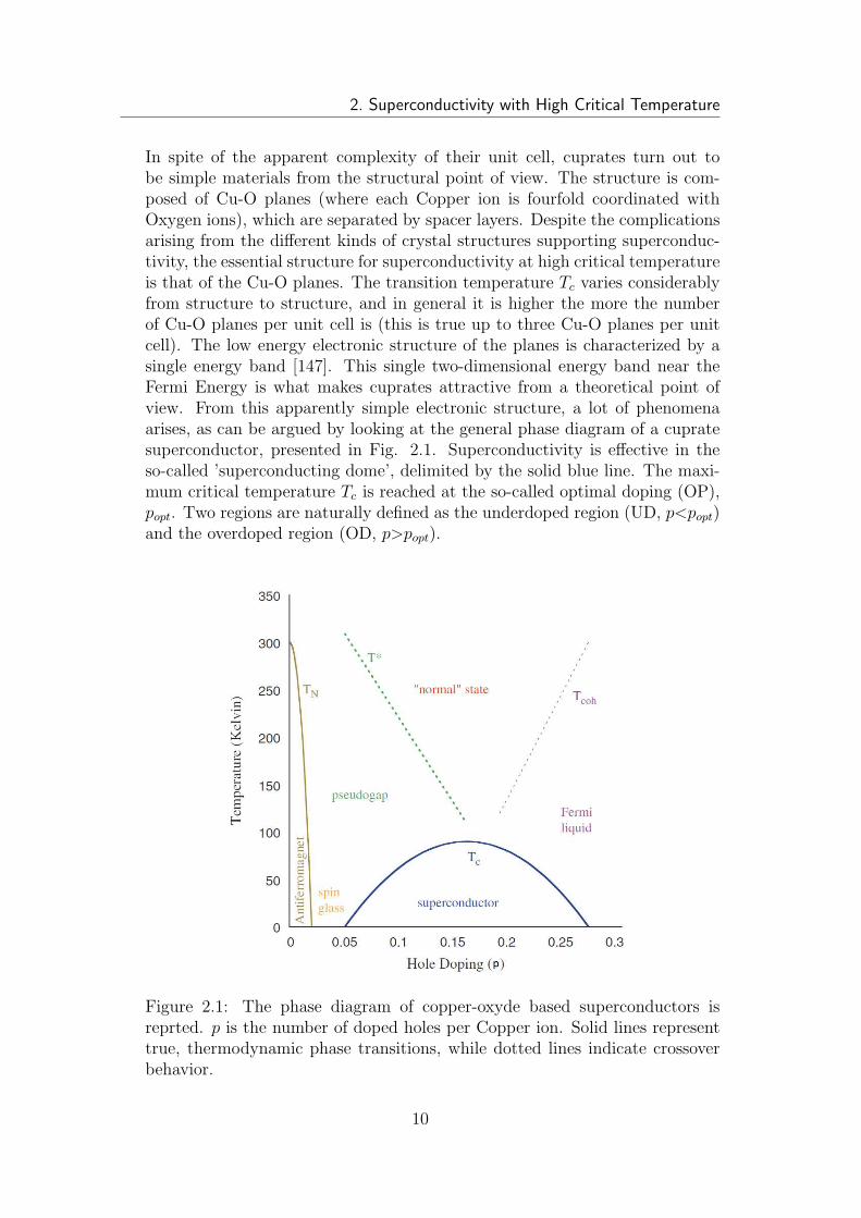
In spite of the apparent complexity of their unit cell, cuprates turn out tobe simple materials from the structural point of view. The structure is com-posed of Cu-O planes (where each Copper ion is fourfold coordinated withOxygen ions), which are separated by spacer layers. Despite the complicationsarising from the different kinds of crystal structures supporting superconduc-tivity, the essential structure for superconductivity at high critical temperatureis that of the Cu-O planes. The transition temperature Tc varies considerablyfrom structure to structure, and in general it is higher the more the numberof Cu-O planes per unit cell is (this is true up to three Cu-O planes per unitcell). The low energy electronic structure of the planes is characterized by asingle energy band [147]. This single two-dimensional energy band near theFermi Energy is what makes cuprates attractive from a theoretical point ofview. From this apparently simple electronic structure, a lot of phenomenaarises, as can be argued by looking at the general phase diagram of a cupratesuperconductor, presented in Fig. 2.1. Superconductivity is effective in theso-called ’superconducting dome’, delimited by the solid blue line. The maxi-mum critical temperature Tc is reached at the so-called optimal doping (OP),popt. Two regions are naturally defined as the underdoped region (UD, p<popt)and the overdoped region (OD, p>popt).
Figure 2.1: The phase diagram of copper-oxyde based superconductors isreprted. p is the number of doped holes per Copper ion. Solid lines representtrue, thermodynamic phase transitions, while dotted lines indicate crossoverbehavior.
10
2.2. Electronic properties of copper-oxide based superconductors
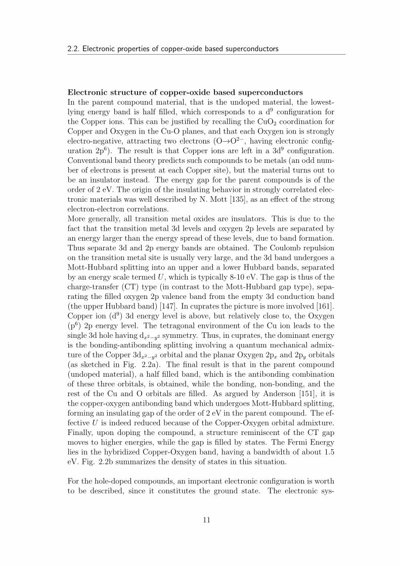
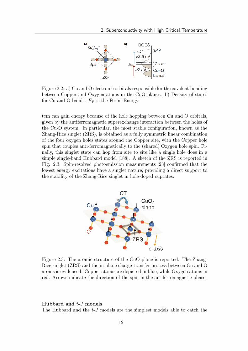
Electronic structure of copper-oxide based superconductorsIn the parent compound material, that is the undoped material, the lowest-lying energy band is half filled, which corresponds to a d9 configuration forthe Copper ions. This can be justified by recalling the CuO2 coordination forCopper and Oxygen in the Cu-O planes, and that each Oxygen ion is stronglyelectro-negative, attracting two electrons (O→O2−, having electronic config-uration 2p6). The result is that Copper ions are left in a 3d9 configuration.Conventional band theory predicts such compounds to be metals (an odd num-ber of electrons is present at each Copper site), but the material turns out tobe an insulator instead. The energy gap for the parent compounds is of theorder of 2 eV. The origin of the insulating behavior in strongly correlated elec-tronic materials was well described by N. Mott [135], as an effect of the strongelectron-electron correlations.More generally, all transition metal oxides are insulators. This is due to thefact that the transition metal 3d levels and oxygen 2p levels are separated byan energy larger than the energy spread of these levels, due to band formation.Thus separate 3d and 2p energy bands are obtained. The Coulomb repulsionon the transition metal site is usually very large, and the 3d band undergoes aMott-Hubbard splitting into an upper and a lower Hubbard bands, separatedby an energy scale termed U , which is typically 8-10 eV. The gap is thus of thecharge-transfer (CT) type (in contrast to the Mott-Hubbard gap type), sepa-rating the filled oxygen 2p valence band from the empty 3d conduction band(the upper Hubbard band) [147]. In cuprates the picture is more involved [161].Copper ion (d9) 3d energy level is above, but relatively close to, the Oxygen(p6) 2p energy level. The tetragonal environment of the Cu ion leads to thesingle 3d hole having dx2−y2 symmetry. Thus, in cuprates, the dominant energyis the bonding-antibonding splitting involving a quantum mechanical admix-ture of the Copper 3dx2−y2 orbital and the planar Oxygen 2px and 2py orbitals(as sketched in Fig. 2.2a). The final result is that in the parent compound(undoped material), a half filled band, which is the antibonding combinationof these three orbitals, is obtained, while the bonding, non-bonding, and therest of the Cu and O orbitals are filled. As argued by Anderson [151], it isthe copper-oxygen antibonding band which undergoes Mott-Hubbard splitting,forming an insulating gap of the order of 2 eV in the parent compound. The ef-fective U is indeed reduced because of the Copper-Oxygen orbital admixture.Finally, upon doping the compound, a structure reminiscent of the CT gapmoves to higher energies, while the gap is filled by states. The Fermi Energylies in the hybridized Copper-Oxygen band, having a bandwidth of about 1.5eV. Fig. 2.2b summarizes the density of states in this situation.
For the hole-doped compounds, an important electronic configuration is worthto be described, since it constitutes the ground state. The electronic sys-
11
2. Superconductivity with High Critical Temperature
Figure 2.2: a) Cu and O electronic orbitals responsible for the covalent bondingbetween Copper and Oxygen atoms in the CuO planes. b) Density of statesfor Cu and O bands. EF is the Fermi Energy.
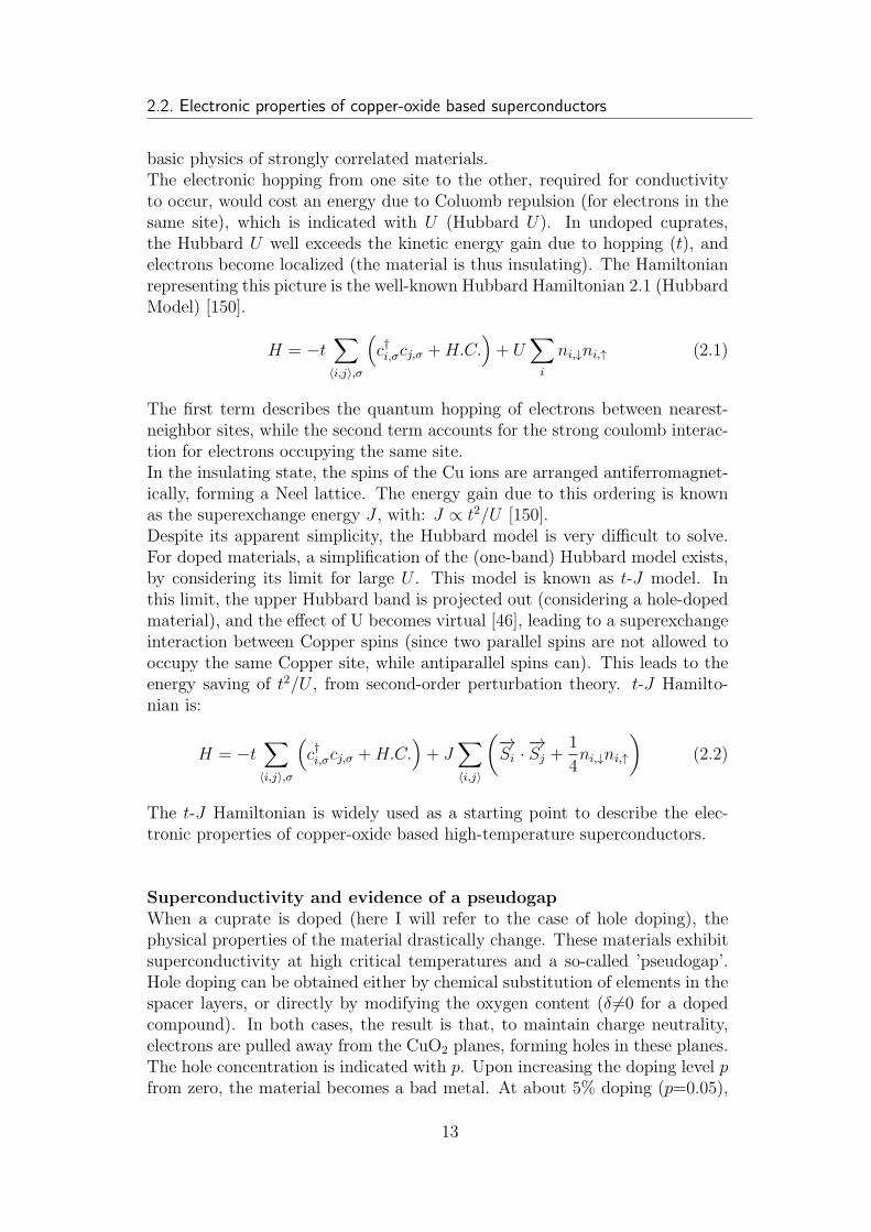
tem can gain energy because of the hole hopping between Cu and O orbitals,given by the antiferromagnetic superexchange interaction between the holes ofthe Cu-O system. In particular, the most stable configuration, known as theZhang-Rice singlet (ZRS), is obtained as a fully symmetric linear combinationof the four oxygen holes states around the Copper site, with the Copper holespin that couples anti-ferromagnetically to the (shared) Oxygen hole spin. Fi-nally, this singlet state can hop from site to site like a single hole does in asimple single-band Hubbard model [188]. A sketch of the ZRS is reported inFig. 2.3. Spin-resolved photoemission measurements [23] confirmed that thelowest energy excitations have a singlet nature, providing a direct support tothe stability of the Zhang-Rice singlet in hole-doped cuprates.
Figure 2.3: The atomic structure of the CuO plane is reported. The Zhang-Rice singlet (ZRS) and the in-plane charge-transfer process between Cu and Oatoms is evidenced. Copper atoms are depicted in blue, while Oxygen atoms inred. Arrows indicate the direction of the spin in the antiferromagnetic phase.
Hubbard and t-J modelsThe Hubbard and the t-J models are the simplest models able to catch the
12
2.2. Electronic properties of copper-oxide based superconductors
basic physics of strongly correlated materials.The electronic hopping from one site to the other, required for conductivityto occur, would cost an energy due to Coluomb repulsion (for electrons in thesame site), which is indicated with U (Hubbard U). In undoped cuprates,the Hubbard U well exceeds the kinetic energy gain due to hopping (t), andelectrons become localized (the material is thus insulating). The Hamiltonianrepresenting this picture is the well-known Hubbard Hamiltonian 2.1 (HubbardModel) [150].
H = −t∑
〈i,j〉,σ
(
c†i,σcj,σ +H.C.)
+ U∑
i
ni,↓ni,↑ (2.1)
The first term describes the quantum hopping of electrons between nearest-neighbor sites, while the second term accounts for the strong coulomb interac-tion for electrons occupying the same site.In the insulating state, the spins of the Cu ions are arranged antiferromagnet-ically, forming a Neel lattice. The energy gain due to this ordering is knownas the superexchange energy J , with: J ∝ t2/U [150].Despite its apparent simplicity, the Hubbard model is very difficult to solve.For doped materials, a simplification of the (one-band) Hubbard model exists,by considering its limit for large U . This model is known as t-J model. Inthis limit, the upper Hubbard band is projected out (considering a hole-dopedmaterial), and the effect of U becomes virtual [46], leading to a superexchangeinteraction between Copper spins (since two parallel spins are not allowed tooccupy the same Copper site, while antiparallel spins can). This leads to theenergy saving of t2/U , from second-order perturbation theory. t-J Hamilto-nian is:
H = −t∑
〈i,j〉,σ
(
c†i,σcj,σ +H.C.)
+ J∑
〈i,j〉
(−→Si ·
−→Sj +
1
4ni,↓ni,↑
)
(2.2)
The t-J Hamiltonian is widely used as a starting point to describe the elec-tronic properties of copper-oxide based high-temperature superconductors.
Superconductivity and evidence of a pseudogapWhen a cuprate is doped (here I will refer to the case of hole doping), thephysical properties of the material drastically change. These materials exhibitsuperconductivity at high critical temperatures and a so-called ’pseudogap’.Hole doping can be obtained either by chemical substitution of elements in thespacer layers, or directly by modifying the oxygen content (δ 6=0 for a dopedcompound). In both cases, the result is that, to maintain charge neutrality,electrons are pulled away from the CuO2 planes, forming holes in these planes.The hole concentration is indicated with p. Upon increasing the doping level pfrom zero, the material becomes a bad metal. At about 5% doping (p=0.05),
13
2. Superconductivity with High Critical Temperature
a superconducting state emerges at low temperatures. The Tc rapidly in-creases with further doping, reaching a maximum value at about 16% doping(p=0.16), termed the optimal doping (OP) level. Further doping makes Tc
to fall to zero, at about 25% doping (p=0.25). Increasing doping further, thematerial becomes an ordinary metal.
The superconducting ground state is isomorphic with that of the BCS the-ory [13, 14], since it consists of a condensate composed of Cooper Pairs [40].The main difference is the symmetry of the gap. In the original BCS theory,the pairs have an s-wave symmetry. On the contrary, the cuprate pairing gaphas a d-wave symmetry (the superconducting gap is no more isotropic in k-space, but it is maximum in the antinodal direction of the Brillouin zone (ΓM),and zero in the nodal direction (ΓY) of the Brillouin zone), as demonstrated byseveral experiments [45, 32]. This fact led to the speculation that the pairingin the cuprates has a different origin from that of conventional superconductors.
Since superconductivity is an instability of the normal state, to understand itsorigin it is mandatory to understand the nature of the normal state from whichit arises. For cuprates, this is where the real controversy begins [140, 137]. In-deed, measurements of the spin response of cuprates below the optimal dopinglevel revealed a reduction in the imaginary part of the low frequency dynamicspin susceptibility, at a temperature larger than Tc [186]. Other magneticsusceptibility measurements [50] showed a suppression of the uniform staticsusceptibility at temperatures significantly higher than Tc. Similar evidenceshas been revealed by the decrease of the spin-lattice relaxation rate in NMR ex-periments on underdoped cuprates [18], and anomalies revealed by tunnellingexperiments [130, 172], c-axis optical conductivity [149], specific heat exper-iments [119] and angle-resolved photoemission experiments [177] have beenreported. On the contrary, this kind of depressions occur in conventional su-perconductors only at Tc. The quenching of these magnetic susceptibilitiesindicates that a sort of pre-pairing is taking place. This also implies the open-ing of an energy gap in the density of states, as evidenced by ARPES studies[49]. In cuprates, the temperature at which these quenching phenomenon be-gin is termed T ∗, while no additional anomaly at Tc are shown: a quenchinganalogous to spin singlet formation of conventional superconductors does notset in at Tc, but at T
∗. In particular, T ∗ increases upon reducing the doping,on the contrary to what happens for Tc. Quenching sets in at higher temper-atures as the Charge-Transfer insulating phase is approached.
This point constitutes the main open question in the HTSC field. No con-sensus exists about the relation existing among the ’spin gap’ or pseudogapand the superconducting phase [89, 137, 173]. By analogy with the conven-tional superconductors case, one possibility is that the pseudogap is also asso-ciated with spin singlet formation. This would indicate a sort of pre-pairing of
14
2.3. Models for the phase diagram
electrons. In this scenario, the pseudogap is thought to be a ’friend’ of super-conductivity [137]. On the contrary, since any instability typically results inan energy gap, and such an energy gap leads by definition to a depression ofthe electronic density of states, some feel the pseudogap does not necessarilyimply spin singlet formation. In these scenarios, the pseudogap is thought assomething unrelated with the phenomenon of superconductivity, or somethingwhich impedes the superconductivity formation (superconductivity ’foe’) [137].
The understanding of the pseudogap phenomenon is intimately connected tothe understanding of the whole phase diagram of the material: each theory forthe phase diagram predicts a different nature for the pseudogap phenomenon.The next section will be devoted to the presentation of the most releveantschemes for the copper-oxide based superconductor phase diagram.
2.3 Models for the phase diagram
The critical parameter that determines the properties of a copper-oxygen basedsuperconductor is the concentration of holes (p) in the Copper-Oxygen planes.The phase diagram obtained by modifying p has been sketched in Fig. 2.1,in the p-T (doping-temperature) parameters space. The UD region is char-acterized by the enigmatic pseudogap phase. This paragraph is aimed to thedescription of the most relevant models for this phase [89, 173].
The models reported in the literature design two main scenarios [137].The first one involves preformed Cooper pairs at temperature T<T ∗, whichbecome phase coherent only for T<Tc. An important theory pointing into thisdirection is contained in a work by Emery and Kivelson [70]. In this theory,the loss of coherence of the condensate at T>Tc is explained in terms of phasefluctuations that, due to the low density of the superconducting carriers ascompared to the standard 3D BCS superconductors, destroy the long rangeorder without breaking the Cooper Pairs. Another theory supporting this firstscenario is based on the notion of spin-charge separation [114, 133]. A singlehole is described as a bound state of a fermionic particle, called spinon, carry-ing only the spin, and a bosonic particle, called holon, carrying only the charge.In strongly correlated electron systems, this dual nature of the charge carriersbecomes more evident, with spinons and holons behaving like independent par-tieles. In a mean-field description, spinons pair together forming a gap in thespin excitation spectrum, interpreted as the pseudogap, while holons undergoBose-Einstein condensation at Tc, making the system superconductive.The opposite scenario is that in which the pseudogap is considered as a phase,characterized by an hidden order, in competition with superconductivity [33,181]. Various candidates for this order have been proposed. In particular,stripe and antiferromagnetic order, d-density wave order (DDW), or currentloops, all break a particular symmetry of the system.
15
2. Superconductivity with High Critical Temperature
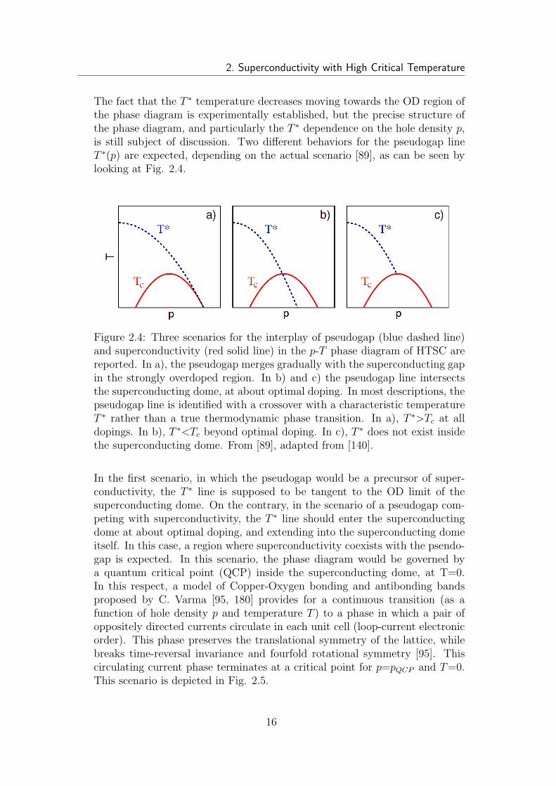
The fact that the T ∗ temperature decreases moving towards the OD region ofthe phase diagram is experimentally established, but the precise structure ofthe phase diagram, and particularly the T ∗ dependence on the hole density p,is still subject of discussion. Two different behaviors for the pseudogap lineT ∗(p) are expected, depending on the actual scenario [89], as can be seen bylooking at Fig. 2.4.
Figure 2.4: Three scenarios for the interplay of pseudogap (blue dashed line)and superconductivity (red solid line) in the p-T phase diagram of HTSC arereported. In a), the pseudogap merges gradually with the superconducting gapin the strongly overdoped region. In b) and c) the pseudogap line intersectsthe superconducting dome, at about optimal doping. In most descriptions, thepseudogap line is identified with a crossover with a characteristic temperatureT ∗ rather than a true thermodynamic phase transition. In a), T ∗>Tc at alldopings. In b), T ∗<Tc beyond optimal doping. In c), T ∗ does not exist insidethe superconducting dome. From [89], adapted from [140].
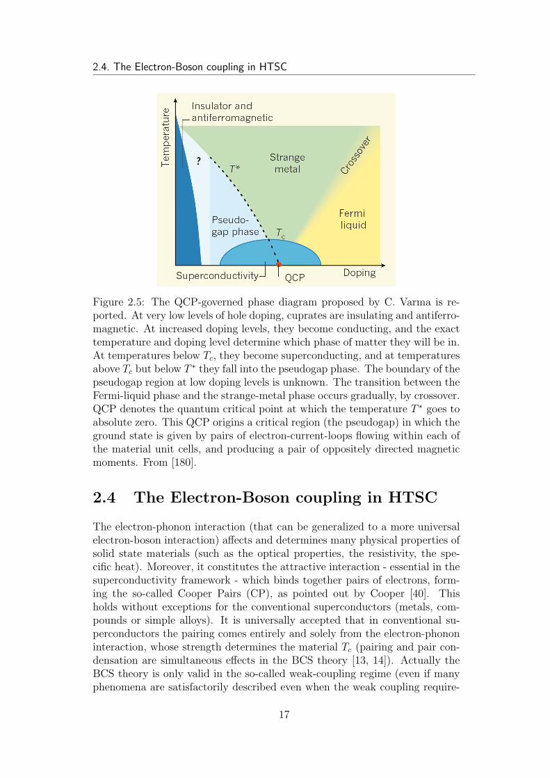
In the first scenario, in which the pseudogap would be a precursor of super-conductivity, the T ∗ line is supposed to be tangent to the OD limit of thesuperconducting dome. On the contrary, in the scenario of a pseudogap com-peting with superconductivity, the T ∗ line should enter the superconductingdome at about optimal doping, and extending into the superconducting domeitself. In this case, a region where superconductivity coexists with the psendo-gap is expected. In this scenario, the phase diagram would be governed bya quantum critical point (QCP) inside the superconducting dome, at T=0.In this respect, a model of Copper-Oxygen bonding and antibonding bandsproposed by C. Varma [95, 180] provides for a continuous transition (as afunction of hole density p and temperature T ) to a phase in which a pair ofoppositely directed currents circulate in each unit cell (loop-current electronicorder). This phase preserves the translational symmetry of the lattice, whilebreaks time-reversal invariance and fourfold rotational symmetry [95]. Thiscirculating current phase terminates at a critical point for p=pQCP and T=0.This scenario is depicted in Fig. 2.5.
16
2.4. The Electron-Boson coupling in HTSC
Figure 2.5: The QCP-governed phase diagram proposed by C. Varma is re-ported. At very low levels of hole doping, cuprates are insulating and antiferro-magnetic. At increased doping levels, they become conducting, and the exacttemperature and doping level determine which phase of matter they will be in.At temperatures below Tc, they become superconducting, and at temperaturesabove Tc but below T ∗ they fall into the pseudogap phase. The boundary of thepseudogap region at low doping levels is unknown. The transition between theFermi-liquid phase and the strange-metal phase occurs gradually, by crossover.QCP denotes the quantum critical point at which the temperature T ∗ goes toabsolute zero. This QCP origins a critical region (the pseudogap) in which theground state is given by pairs of electron-current-loops flowing within each ofthe material unit cells, and producing a pair of oppositely directed magneticmoments. From [180].
2.4 The Electron-Boson coupling in HTSC
The electron-phonon interaction (that can be generalized to a more universalelectron-boson interaction) affects and determines many physical properties ofsolid state materials (such as the optical properties, the resistivity, the spe-cific heat). Moreover, it constitutes the attractive interaction - essential in thesuperconductivity framework - which binds together pairs of electrons, form-ing the so-called Cooper Pairs (CP), as pointed out by Cooper [40]. Thisholds without exceptions for the conventional superconductors (metals, com-pounds or simple alloys). It is universally accepted that in conventional su-perconductors the pairing comes entirely and solely from the electron-phononinteraction, whose strength determines the material Tc (pairing and pair con-densation are simultaneous effects in the BCS theory [13, 14]). Actually theBCS theory is only valid in the so-called weak-coupling regime (even if manyphenomena are satisfactorily described even when the weak coupling require-
17
2. Superconductivity with High Critical Temperature
ment is violated). Its generalization to the strong-coupling regime case is dueto Eliashberg [69, 134, 126], but the main features of the theory remains thesame. Usually, the origin of the net attractive interaction which forms the CPis termed glue. In the BCS theory and its extensions, the glue is given byphonons.Electron-phonon interaction is thus an essential topic to be investigated in theframework of high-temperature superconductivity, to highlight differences orsimilarity with respect to the BCS case. Upon determining the electron-phononcoupling strength in High-Tc materials, it is possible to point out whether thematerial is in the weak or strong coupling regime, and possibly whether otherbosons contribute (entirely or cooperatively) to the pairing. Indeed, no consen-sus has been reached yet on the nature of the (bosonic) glue in the High-Tc: astrong debate is on whether the pairing is due to phonons [44, 56, 113, 120, 167],spin fluctuations [2, 35, 162], or both (bosons of phononic or electronic origin).Many techniques have been exploited to measure the electron-phonon couplingconstant, both in metals and superconductors. Nevertheless, the obtained re-sults are contrasting. Among these techniques, which probe the equilibriumproperties of the material, I may cite ARPES, inelastic neutron scattering, tun-neling spectroscopy, optical conductivity. Extracting information from thesestatic, equilibrium measurements is a task of high difficulty, since complex pro-cedures of data inversion are needed. Reverting to the time-resolved point ofview, the electron-phonon coupling strength can be derived in a straightfor-ward way, instead. The non-equilibrium approach revealed the more direct wayof extracting these information, since it allows to access the temporal domain:the timescale of the return-to-equilibrium of an excited system of electrons andphonons is related (see section 4.3.1) to the electron-phonon coupling strenght.The first experimental results taking advantage of the temporal resolution aredated 1990 for studies with optical measurements [25, 24] and 2007 for studieswith (time-resolved) ARPES [145]. A common model (some alternative mod-els are reported in [96, 75]) employed to extract the electron-phonon couplingis the Two-Temperatures model (and its evolution to the three temperaturesmodel, in the case of strongly correlated systems and anisotropic systems),developed by Anisimov (1974) [10] and Allen (1987) [7]. This model will bedescribed in detail in Chapter 4 (section 3), together with its evolutions. Now,a few words are worth to be spent about the definition of the electron-phononcoupling strength and its relation with the material Tc.
The theory of strong coupling superconductivity is based on the Green’s-function method of the many-body theory, with the theory of strong couplingwhich is a generalization of the theory of normal metals, by Migdal (1957) [126].Some important quantities enter the theory. F (Ω), being Ω the phonon fre-quency, is the phonon density of states (PDOS), which constitutes the phononsspectrum. α2(Ω) is the phonon-frequency-dependent electron-phonon interac-tion. A very common quantity for the theory is the temperature independent,
18
2.4. The Electron-Boson coupling in HTSC
material dependent product α2(Ω)F (Ω), which enters in the definition of the(frequency integrated) electron-phonon coupling constant λ. The expressionα2(Ω)F (Ω) is usually called ’the glue function’. λ represents an effective cou-pling:
λ = 2
∫ ∞
0
α2(Ω)F (Ω)Ω−1dΩ (2.3)
λ is the same as λ 〈Ω0〉, being λ 〈Ωn〉 the moments of α2(Ω)F (Ω), appearingin the superconductivity theory:
λ⟨
Ω0⟩
= 2
∫ ∞
0
[
α2(Ω)F (Ω)Ω−1]
ΩndΩ
Often, a characteristic phonon frequency Ω is defined, as an average overα2(Ω)F (Ω). Following the literature, at least three possibilities are reported:”linear” (Dynes), ”quadratic” (Kresin−Wolf), ”log” (Allen−Dynes, Carbotte):
Ω = 〈Ω〉, Ω = 〈Ω2〉1/2, Ω = 〈ln(Ω)〉. From simple comparison with the BCS-limit case and for the better agreement with the data, the best choice for themean phonon frequency will turn out to be the ”log” one.The mean values come from the expression:
〈f(Ω)〉 = 2
λ
∫ ∞
0
[
α2(Ω)F (Ω)Ω−1]
f(Ω)dΩ
thus:
〈Ω〉 = 2
λ
∫ ∞
0
α2(Ω)F (Ω)dΩ ≡ 2A
λ
⟨
Ω2⟩
=2
λ
∫ ∞
0
α2(Ω)F (Ω)ΩdΩ
〈ln(Ω)〉 = 2
λ
∫ ∞
0
α2(Ω)F (Ω) ln(Ω)dΩ
Expressions for Tc = Tc(λ)The electron-phonon coupling constant λ is an important parameter because itenters the (approximate) expressions determining the material’s Tc, in the var-ious coupling strength formalisms. The problem arises since a correct explicitexpression for Tc depends on the strength of the coupling, thus some limitingcases are analyzed.I start with the weak-coupling regime (λ 6 0.3), in which the BCS theory fullyholds. The BCS result actually reads:
kBTc ≈ 1.13~ΩD exp(−1/N(0)V )
where N(0)V = (λ− µ∗) (λ > µ∗).The net attractive pairing potential V is proportional to an attractive part,
19
2. Superconductivity with High Critical Temperature
λ (originating from the electron-phonon interaction) and a repulsive part, µ∗
(originating from electron-electron Coulomb interaction). In the above formu-lae, N(0) is the density of states (per spin) at the Fermi Energy, and ΩD is theDebye frequency (or a typical phonon frequency) of the material. The BCStheory assumes the coupling is with just one phonon mode (with Ω = ΩD):following the derivation of the above formula, one argues that the correct ex-pression for the mean value Ω is given by the log-average:
Ω = 〈ln(Ω)〉 (2.4)
and that, by definition, in the BCS theory it holds: Ω = ΩD.The above BCS relation indicates that in general Tc is much smaller than thematerial Debye frequency, ΩD. Even in many metallic, conventional supercon-ductors, it turns out that λ is not in the weak-coupling regime (1.4 in Pb, 1.6in Hg), so that new theories should be developed.For larger values of λ (λ . 1.5), i.e., in the strong coupling regime, the re-lation Tc vs λ is given by the famous McMillan formula [125] (later modifiedand improved by Dynes [62] and by Allen&Dynes [8]), which derives from theEliashberg theory:
kBTc ≈~Ω
1.2exp
( −1.04(1 + λ)
λ− µ∗(1 + 0.62λ)
)
(2.5)
This relation reduces to the BCS one in the weak coupling limit, λ ≪ 1. Itshould be noted that in the above expression the coefficients 1/1.2, 1.04, 0.62are the result of a fitting procedure of a more general expression to data fromreal materials: this expression is thus ’semi-phenomenological’.Finally, if the coupling constant λ is large (λ > 1.5), McMillan equation stopsbeing satisfactory, and one should use different expressions for the critical tem-perature Tc (indeed, McMillan equation leads to a saturation of Tc for λ → ∞,while the exact result does not: the effect of a maximum Tc is an artifact ofthe approximations done, and is not intrinsic to the Eliashberg theory fromwhich it follows). A comprehensive review of these relations can be foundin [110, 28]. The conclusion is that, if the material is characterized by largevalues of Ω and λ, it can have a very high Tc. This can be the case whensome high-energy boson-exchange mechanism are operative, as it is the casein copper-oxide based superconductors. Regarding the fact of achieving largevalues of the electron-phonon coupling constant λ, the problem is related tothe framework of lattice or other instabilities, which are not accounted for bythe superconductivity theories. λ cannot increase indefinitely, indeed the lat-tice would surely reach a point when it is no longer stable because of the verylarge electron-phonon interaction, eventually leading to polaron formation. Atpresent, there is no universally accepted and quantitative stability criterion[28].Up to now, I considered for the glue function the expression α2(Ω)F (Ω), indi-cating the frequency dependent electron-phonon interaction. The glue function
20
2.5. Bi2212 Crystal Structure
can be generalized to include other possible scattering mechanisms / channelsfor the electrons, for example, with spin fluctuations, charge fluctuations orloop currents. The coupling between electrons and spin fluctuations is indi-cated in a similar manner as: I2(Ω)χ(Ω). Thus, the total glue can be writtenas: Π(Ω) = α2(Ω)F (Ω) + I2(Ω)χ(Ω) + .... In this framework, λ assumes themore general meaning of an electron-boson coupling constant. A strong debateexists on whether the electron-phonon interaction alone can provide the highcritical temperatures typical of the cuprate superconductors [110].Considering the total glue function Π(Ω) as a source of pairing for electronsis the ultimate step for the coupling theories which propose bosonic ’media-tors’ for the formation of Cooper Pairs. It must be noted that these theories,which consider a ”retarded” attraction mediated by the exchange of bosonicexcitations forming the bosonic glue, and not the only ones that have been pro-posed. They are set against the theories for which the pairing comes directlyby the (”non-retarded”) Coulomb interaction, without the need of mediators[151, 9, 146].The presented approximate relations for Tc = Tc(λ, Ω) are of paramount im-portance since they relate the material Tc to average values of the quantityΠ(Ω), i.e., λ and Ω. In section 4.3 I will present some models which allowto estimate, from time-resolved pump-probe measurements, the parameter λ.The valuse for λ obtained by measurements in the time-domain can be com-pared to the values obtained by relation 2.3, which integrates the total GlueFunction Π(Ω) obtained from static optical measurements (section 3.7.2).
2.5 Bi2212 Crystal Structure
Bi2Sr2Cam−1CumO2m+4+δ, often abbreviated with BSCCO (Bismuth-Strontium-Calcium-Copper-Oxyde) to highlight the chemical elements it contains, is oneof the most important members of the high critical temperature copper oxidebased (cuprate) superconductors. In the above formula, m indicates the num-ber of Copper-Oxygen (Cu-O2) planes in the conventional unit cell of the ma-terial, while δ indicates the doping level, obtained through modification of theOxygen concentration. In the BSCCO compound, the variation of the Oxygenstoichiometry δ results in an effective hole-doping mechanism. Cuprates arecharacterized by a layered structure, with Cu-O2 planes separated by spacerlayers that act as charge reservoirs.Among the more than 20 distinct phases in which the BSCCO compound canbe synthetized, differing for the stoichiometric ratios and the growing process,only three show high temperature superconductivity properties. They are indi-cated with Bi2201 (the one-plane Copper-Oxygen compound, having Tcmax=20K), Bi2212 (the two-planes Copper-Oxygen compound, having Tcmax=90 K),and Bi2223 (the three-planes Copper-Oxygen compound, having Tcmax=110K). The main difference between the three compound resides only in the num-ber m of Cu-O planes contained in the conventional unit cell.
21
2. Superconductivity with High Critical Temperature
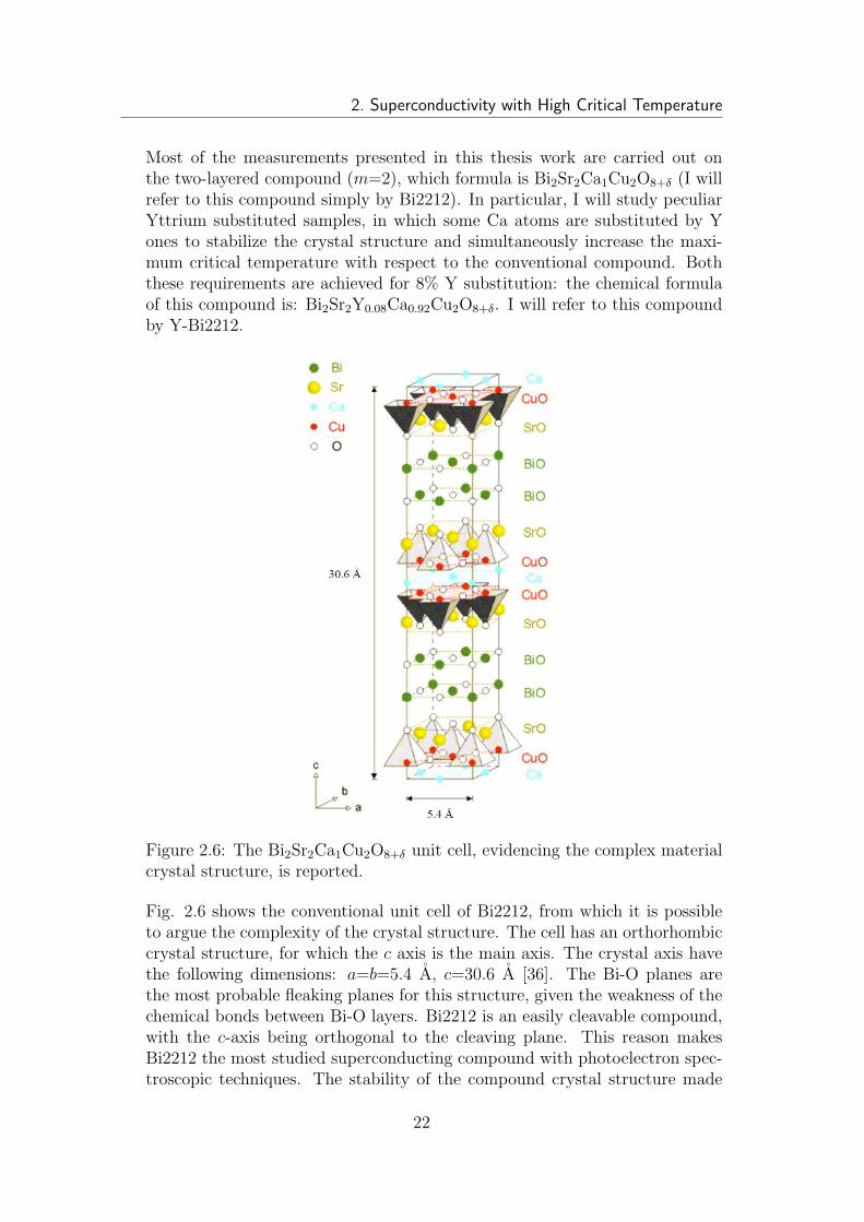
Most of the measurements presented in this thesis work are carried out onthe two-layered compound (m=2), which formula is Bi2Sr2Ca1Cu2O8+δ (I willrefer to this compound simply by Bi2212). In particular, I will study peculiarYttrium substituted samples, in which some Ca atoms are substituted by Yones to stabilize the crystal structure and simultaneously increase the maxi-mum critical temperature with respect to the conventional compound. Boththese requirements are achieved for 8% Y substitution: the chemical formulaof this compound is: Bi2Sr2Y0.08Ca0.92Cu2O8+δ. I will refer to this compoundby Y-Bi2212.
Figure 2.6: The Bi2Sr2Ca1Cu2O8+δ unit cell, evidencing the complex materialcrystal structure, is reported.
Fig. 2.6 shows the conventional unit cell of Bi2212, from which it is possibleto argue the complexity of the crystal structure. The cell has an orthorhombiccrystal structure, for which the c axis is the main axis. The crystal axis havethe following dimensions: a=b=5.4 A, c=30.6 A [36]. The Bi-O planes arethe most probable fleaking planes for this structure, given the weakness of thechemical bonds between Bi-O layers. Bi2212 is an easily cleavable compound,with the c-axis being orthogonal to the cleaving plane. This reason makesBi2212 the most studied superconducting compound with photoelectron spec-troscopic techniques. The stability of the compound crystal structure made
22
2.5. Bi2212 Crystal Structure
this compound one of the most studied in general, together with the YBCOcopper oxide based superconductor. Bi-O planes are also the planes in whichthe extra Oxygen atoms due to the doping modify the hole concentration. Thedoping content δ strongly affects the physical properties of BSCCO. Indeed, forδ = 0, this compound is an antiferromagnetic charge transfer insulator. It isonly for δ > 0 that the system becomes a (bad) metal. Moreover, it is only forδ > δc, being δc a critical doping level, that the system undergoes the supercon-ducting transition, when cooled. The superconductivity then disappears if amaximum doping level, indicated with δl, is crossed. Thus, superconductivityexists only for a limited range of doping concentrations, namely δc 6 δ 6 δl.The doping level for which the compound exhibits its maximum critical tem-perature, Tcmax, is called optimal doping level, δopt. δopt=0.16 in Bi2212.
The critical temperature is related to the oxygen doping level p by the phe-nomenological formula [148]:
Tc(p) = Tcmax
[
1− 82.6(p− 0.16)2]
(2.6)
being Tcmax=96 K for our compound.
All cuprates are known for their high anisotropic properties. As an exam-ple of this, I may cite the electrical resistivity of Bi2212, equal to ρc ≈2 Ω·cmalong the c axis and equal to ρab ≈10−4 Ω·cm in the ab plane [43]. In the super-conducting phase, both ρc and ρab drop below the measurability level. Similaranisotropy properties can be found in the thermical conductivity properties.The coherence length, with ξab ≈30ξc [55], is the manifestation of the materialanisotropy in the superconducting phase.
The values of the electronic and lattice specific heats for these samples, thatwill be employed in the following chapters of this thesis, has been taken from[94, 118]. For simulations involving the specific heat of the Bi2212 compound(like those reported in Chapters 4, 6, 7, 8), it is important to remember thatone Bi2212 mole contains NA=6.022·1023 Bi2212 molecules, with every Bi2212molecule composed of 15 atoms (2 Bismuth, 2 Strontium, 1 Calcium, 2 Copper,8 Oxygen). The volume of one Bi2212 primitive cell equals 223 A3, while itsdenisty equals 6.56 g/cm3, corresponding to 891.15 g/mol.
2.5.1 The Yttrium-doped Bi2212
In Bi2Sr2CaCu2O8+δ, cation disorder at the Sr crystallographic site strongly af-fects the maximum attainable value for Tc [68]. By minimizing Sr site disorderat the expense of Ca site disorder, it has been demonstrated that the Tc of the
23
2. Superconductivity with High Critical Temperature
two-layered Bismuth-based material can be increased up to 96 K. In particular,this important advance has been achieved by growing a compound in whichCa has been substituted by Y, namely: Bi2Sr2YyCa1−yCu2O8+δ. Tc,max=96K has been obtained for y=0.08 (i.e., for 8% Y substitution). The chemicalformula for this compound is: Bi2Sr2Y0.08Ca0.92Cu2O8+δ (Y-Bi2212). Substi-tution of Y for Ca also helps to enforce Bi:Sr stoichiometry, which reduceschemical inhomogeneities. Moreover, this compound is as easy to prepare asordinary, nonstoichiometric Bi2212. For our purposes it is worth to note thatthe electronic properties of this compound are similar to those of the mostknown Bi2212.
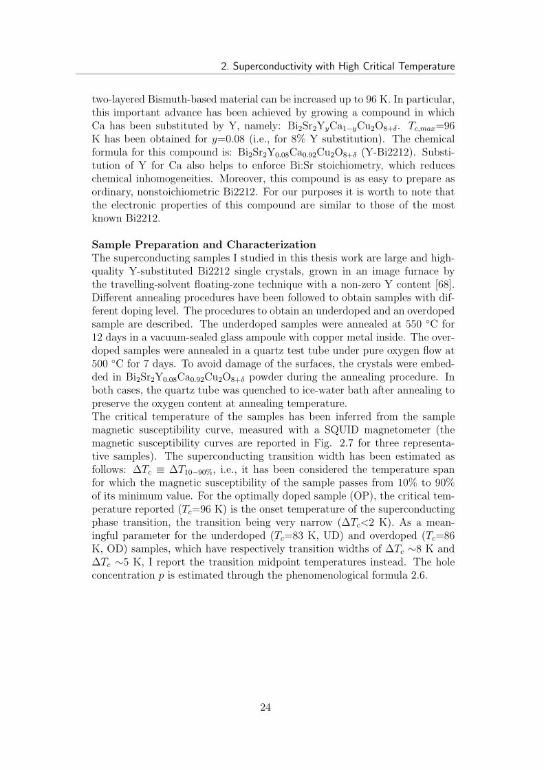
Sample Preparation and CharacterizationThe superconducting samples I studied in this thesis work are large and high-quality Y-substituted Bi2212 single crystals, grown in an image furnace bythe travelling-solvent floating-zone technique with a non-zero Y content [68].Different annealing procedures have been followed to obtain samples with dif-ferent doping level. The procedures to obtain an underdoped and an overdopedsample are described. The underdoped samples were annealed at 550 C for12 days in a vacuum-sealed glass ampoule with copper metal inside. The over-doped samples were annealed in a quartz test tube under pure oxygen flow at500 C for 7 days. To avoid damage of the surfaces, the crystals were embed-ded in Bi2Sr2Y0.08Ca0.92Cu2O8+δ powder during the annealing procedure. Inboth cases, the quartz tube was quenched to ice-water bath after annealing topreserve the oxygen content at annealing temperature.The critical temperature of the samples has been inferred from the samplemagnetic susceptibility curve, measured with a SQUID magnetometer (themagnetic susceptibility curves are reported in Fig. 2.7 for three representa-tive samples). The superconducting transition width has been estimated asfollows: ∆Tc ≡ ∆T10−90%, i.e., it has been considered the temperature spanfor which the magnetic susceptibility of the sample passes from 10% to 90%of its minimum value. For the optimally doped sample (OP), the critical tem-perature reported (Tc=96 K) is the onset temperature of the superconductingphase transition, the transition being very narrow (∆Tc<2 K). As a mean-ingful parameter for the underdoped (Tc=83 K, UD) and overdoped (Tc=86K, OD) samples, which have respectively transition widths of ∆Tc ∼8 K and∆Tc ∼5 K, I report the transition midpoint temperatures instead. The holeconcentration p is estimated through the phenomenological formula 2.6.
24
2.5. Bi2212 Crystal Structure
Figure 2.7: The magnetic susceptibility curves for threeBi2Sr2Y0.08Ca0.92Cu2O8+δ samples are reported. The number of dopedholes per Copper ion, p, is: p=0.128 for the UD sample, p=0.16 for the OPsample, p=0.197 for the OD sample.
25
2. Superconductivity with High Critical Temperature
26
Chapter 3Equilibrium Spectroscopy
3.1 Introduction
This chapter reports the description of the static optical properties of HTSC.I’ll start with a review of the definitions and models which I will exploit in thesubsequent chapters of this work. In particular, the main focus will be about arecently developed version of the Extended Drude formalism, which takes intoaccount the presence of a gap in the density of states (non-constant densityof states). A brief review of the relationships among optical properties and ofthe important sum rules will follow. Finally, the results of the model fitting tothe experimental dielectric functions of Y-Bi2212 at T=300 K, T=100 K andT=20 K will be illustrated. The first case allowed us to extract the materialbosonic glue, while data at T=100 K allows to discuss the role of a non-constantdensity of states.
3.2 The dielectric function ǫ(ω)
The dielectric function, ǫ(ω), is a material-dependent complex function de-scribing, in the frequency domain, the response of a material to an externally
applied electric field−→E (ω):
−→D(ω) = ǫ(ω)
−→E (ω), being
−→D(ω) the effective elec-
tric field (also known as displacement field),−→D(ω) = ǫ0
−→E (ω) +
−→P (ω). Here
ǫ0 is the vacuum permittivity (ǫ0=8.85·10−12 F/m), and−→P (ω) the (material
dependent) polarization. ω is the frequency of the electric field. ǫ(ω) is aresponse function, since it relates the characteristic response of a system tothe externally applied stimulus. Being a response function, it is causal, in thesense that no effect can occur before the cause. As we will see, this intuitiverequirement brings very important results. In one sense, the dielectric functionestablishes the link between the macroscopic world and the microscopic one.From the macroscopic point of view, starting from ǫ(ω), all the optical prop-erties can be calculated (see section 3.3). In particular, the reflectivity R(ω),
27
3. Equilibrium Spectroscopy
the transmissivity T(ω), the complex index of refraction n(ω), the complexoptical conductivity σ(ω) and the penetration depth α(ω) can be all inferredfrom ǫ(ω). From the microscopic point of view, ǫ(ω) is related to the opti-cal electronic transitions in the material, that depend on the specific materialband structure. As a consequence, a detailed knowledge of this function wouldprovide unique information about the underlying electronic properties of thematerials.A detailed description of the key concepts to interpret the electronic opticalproperties of solids can be found in [185, 59], together with notions on theexperimental techniques, the principles of spectroscopy, and the measurementconfigurations. In the field of equilibrium optical spectroscopy, among themost important experimental works in which the optical properties of noblemetals and transition metal oxydes are measured and interpreted, I can cite[65, 66, 67, 39, 155]. A review of the electrodynamics of copper-oxyde-basedhigh-temperature superconductors can be found in [15], while a recent reviewof the optical properties of strongly correlated electron materials is [16].In principle, the dielectric function ǫ(ω) can be determined from first principles(with the exact electronic structure calculation, but this is the case only forvery simple materials [121]), it can be determined with calculations using Den-sity Functional Theory (DFT), for metals, or Dynamical Mean Field Theory(DMFT), for strongly correlated systems, or, finally, it can be modeled, as itis very often the case. Sections 3.4 and 3.5 are enterely devoted to providean accurate description of the models developed to this aim, and that are themost often used in the literature [15, 16, 179, 90]. An accurate reproductionof the experimentally measured equilibrium dielectric function of Y-Bi2212 byusing these models constituted the preliminary task of my work. Results ofthis analysis are presented in section 3.7.
3.3 Optical Properties
In this section I report some useful expressions relating the dielectric functionǫ(ω) = ǫ1(ω) + iǫ2(ω) to other optical quantities of interest:
• The refraction index n(ω) = n1(ω) + in2(ω) of a non-magnetic materialis:
n(ω) =√
ǫ(ω) (3.1)
• The optical conductivity σ(ω) = σ1(ω) + iσ2(ω) is:
σ(ω) = iω
4π(ǫ(ω)− 1) (3.2)
28
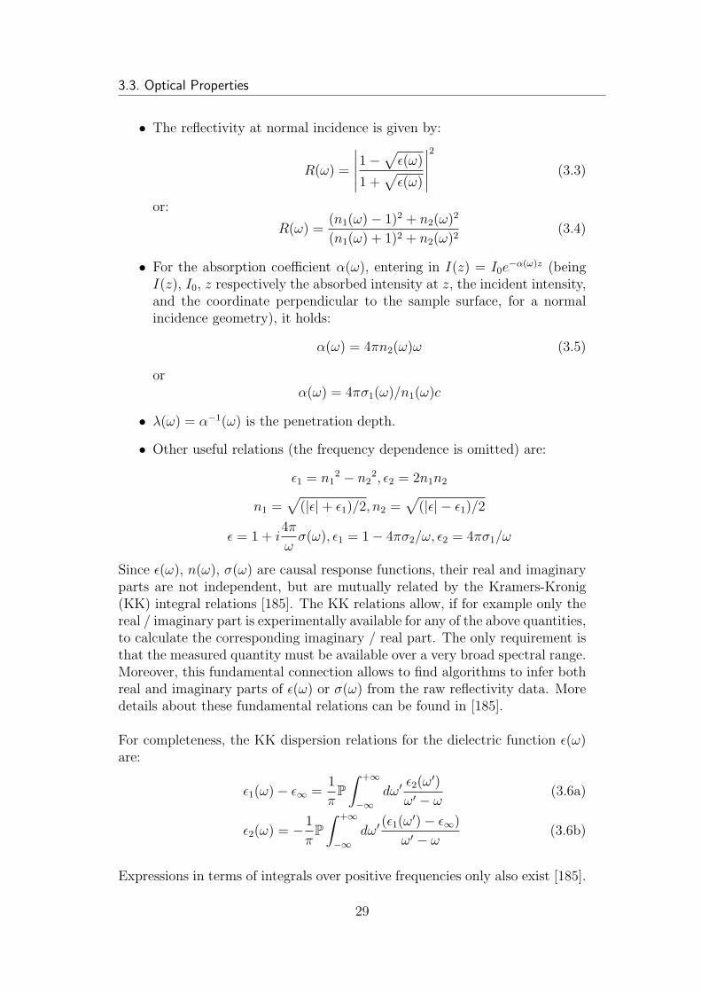
3.3. Optical Properties
• The reflectivity at normal incidence is given by:
R(ω) =
∣
∣
∣
∣
∣
1−√
ǫ(ω)
1 +√
ǫ(ω)
∣
∣
∣
∣
∣
2
(3.3)
or:
R(ω) =(n1(ω)− 1)2 + n2(ω)
2
(n1(ω) + 1)2 + n2(ω)2(3.4)
• For the absorption coefficient α(ω), entering in I(z) = I0e−α(ω)z (being
I(z), I0, z respectively the absorbed intensity at z, the incident intensity,and the coordinate perpendicular to the sample surface, for a normalincidence geometry), it holds:
α(ω) = 4πn2(ω)ω (3.5)
orα(ω) = 4πσ1(ω)/n1(ω)c
• λ(ω) = α−1(ω) is the penetration depth.
• Other useful relations (the frequency dependence is omitted) are:
ǫ1 = n12 − n2
2, ǫ2 = 2n1n2
n1 =√
(|ǫ|+ ǫ1)/2, n2 =√
(|ǫ| − ǫ1)/2
ǫ = 1 + i4π
ωσ(ω), ǫ1 = 1− 4πσ2/ω, ǫ2 = 4πσ1/ω
Since ǫ(ω), n(ω), σ(ω) are causal response functions, their real and imaginaryparts are not independent, but are mutually related by the Kramers-Kronig(KK) integral relations [185]. The KK relations allow, if for example only thereal / imaginary part is experimentally available for any of the above quantities,to calculate the corresponding imaginary / real part. The only requirement isthat the measured quantity must be available over a very broad spectral range.Moreover, this fundamental connection allows to find algorithms to infer bothreal and imaginary parts of ǫ(ω) or σ(ω) from the raw reflectivity data. Moredetails about these fundamental relations can be found in [185].
For completeness, the KK dispersion relations for the dielectric function ǫ(ω)are:
ǫ1(ω)− ǫ∞ =1
πP
∫ +∞
−∞
dω′ ǫ2(ω′)
ω′ − ω(3.6a)
ǫ2(ω) = − 1
πP
∫ +∞
−∞
dω′ (ǫ1(ω′)− ǫ∞)
ω′ − ω(3.6b)
Expressions in terms of integrals over positive frequencies only also exist [185].
29
3. Equilibrium Spectroscopy
3.4 Drude and Lorentz dielectric functions
The most common models for reproducing a generic dielectric function are theclassical Lorentz and Drude models. The Lorentz model is applicable to insu-lators, while the Drude model is applicable to free electron metals. They candescribe respectively the effect of optical transitions on the optical properties,for direct interband transitions (transitions for which the final state of an elec-tron lies in a different band, but with no change in the k-vector) and intrabandtransitions (transitions in the same band; in particular, the conduction band).These classical models, describing the response to an external electric field−→E (ω) of a bound or a free electron in a solid, have a simple derivation. Theidea at their base, in an intuitive and classical picture, is to describe the elec-tronic response to an electric field with an harmonic oscillator, for an electronin an atom or solid. The electron with mass m and charge e, when immersed inan electric field E(t) =
∫∞
−∞E(ω)e−iωtdω, is subject to a driving force −eE(ω).
The restoring force is modeled through Hooke’s law: −mω20r. Here ω0 is not
the electron binding energy in the atom / solid, but rather the energy differ-ence of an allowed optical transition. In the Drude model, ω0 = 0, since thereexist no threshold for absorption, for a conduction electron in a free electronmetal. Finally, the electron is subject to a viscous damping (representing anenergy loss mechanism arising from various scattering mechanisms) modeledas: −mγ(dr/dt). This damping term is responsible for the fact that the in-duced polarizability is complex, thus it differs in phase from the driving field,at all frequencies. In the case of a nearly free electron metal (Drude model),γ = 1/τ , being τ the mean free time between collisions, originated from the or-dinary scattering of electrons with impurities and phonons, which is the samescattering mechanism determining the value and temperature-dependence ofthe electrical resistivity. Solving the motion equation, and and calculating the
polarization−→P (ω), the dielectric functions for the Lorentz (ǫL(ω)) and Drude
(ǫD(ω)) models result. They can be written as:
ǫL(ω) = 1 +ωp
2
(ω02 − ω2)− iγω
=
[
1 + ωp2 (ω0
2 − ω2)
(ω02 − ω2)2 + γ2ω2
]
+
+ i
[
ωp2 γω
(ω02 − ω2)2 + γ2ω2
] (3.7)
ǫD(ω) = 1− ωp2
ω2 + iγω=
[
1− ωp2 1
ω2 + γ2
]
+ i
[
ωp2 γ/ω
ω2 + γ2
]
(3.8)
where ωp is the oscillator plasma frequency, defined as follows: ωp2 = 4πNe2/m.
In a realistic situation, the two models must be used simultaneously: the Drudemodel reproduces the low-energy side of the dielectric function, associated tothe metallic behavior; the Lorentz model reproduces the high-energy part ofthe dielectric function, associated to interband transitions. Usually, a cut-off
30
3.5. Extended Drude Model
frequency, ωc, is defined as the frequency at the crossing of the two behaviors.This choice is arbitrary and lead to some debate, since the tail of the Drudecontribution extends well beyond ωc. In doped cuprates, this cutoff is usuallyplaced at about 10000 cm−1, i.e., 1.25 eV [138]. Thus, in general, a modeldielectric function comprises both kinds of oscillators; moreover, often a sumof different Lorentz oscillators is considered, to take into account the fact thatmany optical transitions from discrete bands or levels can be allowed. Theresulting model dielectric function ǫ(ω) is written as:
ǫ(ω) = ǫD(ω) +m∑
i=1
ǫLi(ω) = ǫ1(ω) + iǫ2(ω) (3.9)
where i labels the allowed interband transitions. ǫ1(ω) and ǫ2(ω) are:
ǫ1(ω) = ǫ∞ − ωp02 1
ω2 + γ02+
m∑
i=1
ωpi2 (ω0i
2 − ω2)
(ω0i2 − ω2)2 + γi2ω2
(3.10)
ǫ2(ω) = ωp02 γ0/ω
ω2 + γ02+
m∑
i=1
ωpi2 γiω
(ω0i2 − ω2)2 + γi2ω2
(3.11)
In ǫ1(ω), ǫ∞ takes into account the effect of high-energy interband transitions,which are usually not included in the model. Ideally, if one would include allthe possible interband transitions, it would result: ǫ∞=1.While the Lorentz model is widely used to reproduce the interband transitionsin a variety of materials, the Drude model fails in reproducing the low-energyoptical behavior in systems where a strong electron-boson interaction is present[6, 5, 105]. The conventional Drude model is strictly valid only for simple met-als, having a constant density of states at EF and a frequency-independentscattering time τ (the impurity scattering). To interpret the low-energy opti-cal properties of strongly correlated materials, in which quasiparticles stronglyinteract with bosonic excitations (phonons or other bosonic excitations of elec-tronic origin) or a gap in the density of states opens [166], an extended formal-ism has been developed by Allen [6, 5], namely, the Extended Drude Model(EDM). On its basis the optical properties of strongly correlated materials aretoday successfully interpreted [15, 16]. In the next section the EDM in itsvarious forms will be discussed.
3.5 Extended Drude Model
Unless a very simple metallic material is considered, in which conduction bandelectrons are almost non-interacting with phonons, the Drude model revealsits limits in correctly reproducing the optical properties. Within the Drudemodel, the effect of band structure is accounted for by considering an effective
31
3. Equilibrium Spectroscopy
mass m∗ instead of the bare electron mass m in the expression of the plasmafrequency, while the scattering from impurities is accounted for by the damp-ing term γ, which I will now rename as γimp.When the electrons are interacting with some bosonic excitations (electron-boson interaction), characterized by a typical spectral distribution, the scat-tering process and the electron lifetime become strongly frequency-dependent.Sources of electron-boson interaction can be the electron-phonon coupling (ei-ther anisotropic, with prefential, strongly coupled modes, or with the wholelattice), or an interaction with bosons of electronic origin, namely, antiferro-magnetic spin fluctuations [2, 35, 141] or current loops [180]. This effect isparticularly severe in strongly correlated systems and cuprates, where part ofthe total electron-boson interaction is thought to be the source of couplingfor the electrons forming pairs, in the scenario in which the attractive interac-tion is ’retarded’, i.e., mediated by virtual bosonic excitations in the solid [127].
This physics is included in the EDM, which considers the novel sources of scat-tering, and accounts for a frequency-dependent scattering rate and the renor-malization of the electron effective mass due to the interaction. In a metallicsystem, the physical processes responsible for renormalization of electroniclifetimes and effective masses, are included in the description of the opticalproperties in a phenomenologic way, by replacing the frequency-independentscattering time τ (where τ−1 = γ) with a complex and frequency-dependentscattering time, τ(ω), given by:
τ−1 ⇒ τ−1(ω) = τ−1(ω)− iωλ(ω)
where λ(ω) = m∗
m− 1.
The quantities τ−1(ω) and 1+ λ(ω) describe the frequency-dependent scatter-ing rate and the mass-enhancement of the electronic excitations, which are dueto many-body interactions. The quantity τ−1(ω) is equivalently termed opticalself-energy, Σopt(ω, T ), or memory function, M(ω, T ) (we explicit the tempera-ture dependence). In the literature, the definition of M(ω, T ) is not univoque.In particular, the most common definitions are: M(ω, T ) = τ−1(ω) [15, 132,174], M(ω, T ) = iM(ω, T ) = iτ−1(ω) [179, 16], or finally −2Σopt(ω, T ) =
M(ω, T ) [91, 92]. To avoid confusion, in the following I will use the first defi-nition, with:
M(ω, T ) = M1(ω, T ) + iM2(ω, T ) = 1/τ(ω, T ) + iωλ(ω, T )
In this case, the dielectric function ǫD(ω, T ) is given by:
32
3.5. Extended Drude Model
ǫD(ω, T ) = 1− ωp2
ω(ω + i/τ(ω, T ))= 1− ωp
2
ω(ω + iM(ω, T ))=
= 1− ωp2
ω(ω(1 + λ(ω, T )) + i/τ(ω, T ))
(3.12)
In terms of the optical conductivity σ(ω, T ), which is most often used in theliterature, one obtains:
σD(ω, T ) =1
4π
ωp2
1/τ(ω, T )− iω=
1
4π
ωp2
M(ω, T )− iω=
=1
4π
ωp2
1/τ(ω, T )− iω(1 + λ(ω, T ))
(3.13)
This can be rewritten in the conventional Drude form as:
σ(ω, T ) =1
4π
ω∗2p (ω, T )
1/τ ∗(ω, T )− iω
after introducing the renormalized scattering time and plasma frequency:1/τ ∗(ω, T ) = 1/τ(ω, T )[1 + λ(ω, T )], ω∗2
p (ω, T ) = ω2p/[1 + λ(ω, T )].
The following relations holds, which indicates that 1/τ(ω, T ) and 1 + λ(ω, T )are Kramers-Kronig related:
1/τ(ω) =ω2p
4πRe
(
1
σ(ω)
)
1 + λ(ω) = −ω2p
4π
1
ωIm
(
1
σ(ω)
)
After having illustrated the phenomenology at the base of the EDM, I focus onthe microscopic scattering mechanisms at the basis of τ(ω). In the following,various versions of the formalism, which differs in the way the complex andfrequency dependent scattering time τ(ω) is expressed, are briefly described.
3.5.1 Extended Drude Model in the case of weak electron-phonon coupling
The EDM form illustrated in this section is the first derived version, as pro-posed by Allen in 1971 [6], to describe the far-infrared optical properties inmetals characterized by a non-negligible, though weak, electron-phonon inter-action. The aim of the work was to stimulate a debate about the differencesin the optical behavior of normal and supeconducting materials. In fact, itwill be soon clear how from this theory the electron-phonon coupling functioncan be extracted. The first applications of this theory [5] allowed to correctlyinterpret the departures of NiSb and NiAs intraband optical spectra from the
33
3. Equilibrium Spectroscopy
conventional Drude behavior. Allen original theory, valid in the limit T → 0,was later generalized for finite T by Shulga [167]. The theory valid for weakelectron-phonon coupling was derived within second order perturbation theory.This theory accounts for the additional photon absorption, with respect to aconventional metal, arising from second order processes involving the creationof both a phonon and an electron-hole pair. This approach is equivalent to afirst iteration of the collision term in the Holstein-type Boltzmann equation,and is not as accurate as the full solution of the Boltzmann equation [6].
Within these approximations, the memory function M(ω, T ) can be written asa convolution integral between a transport spectral function, α2
trF (Ω), and aKernel function, K
(
ω2πT
, Ω2πT
)
, which describes the thermal dependence of thephononic excitations coupled with the electrons:
M(ω, T ) = −2
∫ ∞
0
α2trF (Ω)K
(
ω
2πT,
Ω
2πT
)
dΩ (3.14)
where the (material independent) Kernel function writes:
K(x, y) =i
y+
y − x
x[Ψ(1− ix+ iy)−Ψ(1 + iy)]
+
y + x
x[Ψ(1− ix− iy)−Ψ(1− iy)]
(3.15)
where Ψ(z) are the Digamma functions, x = ω/2πT , y = Ω/2πT .The quantity α2
trF (Ω) is related to the transport properties of the material.In 1999 Marsiglio [122] found a method to directly determine α2
trF (Ω) fromspectroscopic data, with an inversion procedure:
α2trF (Ω) =
1
2π
ω2p
4π
d2
dω2Re
(
1
σ(ω)
)
It must be pointed out that the quantity α2trF (Ω) is different from the more
conventional α2F (Ω).Within the weak-coupling formalism, extended to finite temperatures, the tem-perature and frequency-dependent scattering time τ(ω, T ) is written as:
1
τ(ω, T ) =
π
ω
∫ ∞
0
dΩα2trF (Ω)
[
2ωcoth
(
Ω
2T
)
− (ω + Ω)coth
(
ω + Ω
2T
)
+
+(ω − Ω)coth
(
ω − Ω
2T
)
+ γimp
]
(3.16)
I numericaaly verified this model being KK consistent.
34
3.5. Extended Drude Model
3.5.2 Extended Drude Model in the case of strong electron-phonon coupling
In the case of strong electron-phonon coupling, the Extended Drude formalismis derived starting from the Holstein theory for normal metals, which is themost complete theory for metals. Considering the Kubo formula and usingcomplex diagrammatic techniques to evaluate the electron and phonon ther-mal Green’s functions, if one omits vertex corrections (Migdal approximation),the Memory function M(ω, T ) results:
iM(ω, T ) + ω
ω=
∫ +∞
−∞
f(ξ, T )− f(ξ + ω, T )
ω + Σ∗(ξ, T )− Σ(ξ + ω, T ) + iγimp
dξ
−1
(3.17)
M(ω, T ) = −iω
∫ +∞
−∞
f(ξ, T )− f(ξ + ω, T )
ω + Σ∗(ξ, T )− Σ(ξ + ω, T ) + iγimp
dξ
−1
+iω (3.18)
where f is the Fermi-Dirac distribution, Σ(ω, T ) and Σ∗(ω, T ) respectively theelectron and hole self-energies. These are obtained averaging Σ(ω, k, T ) overthe Fermi surface and assuming a constant density of states at EF .The optical self energy M(ω, T ) and the one-particle electronic self-energyΣ(ω, T ) (averaged over the Fermi surface) have the same analytical proper-ties. However, they are conceptually different quantities. Σ(ω, T ) is a quantitymeasured by a photoemission experiment, since this technique probes the sin-gle particle excitations of the (N-1) particle system, which can be describedin terms of the spectral function and the single particle self energy. On thecontrary, an optical experiment looks at the particle-hole excitations of an Nparticle system, and gives information about the joint particle-hole density ofstates.The electron self-energy Σ(ω, T ) is calculated through a convolution integralbetween the coupling function α2F (Ω) and a kernel function L(ω,Ω, T ), in thefollowing way:
Σ(ω, T ) =
∫ ∞
0
α2F (Ω)L(ω,Ω, T )dΩ (3.19)
The kernel function L(ω,Ω, T ) in this formalism is written as:
L(ω,Ω, T ) =
∫[
n(Ω′) + f(Ω)
Ω− ω + Ω′ + iδ+
1 + n(Ω′)− f(Ω)
Ω− ω − Ω′ − iδ
]
dΩ′ (3.20)
n(Ω) being the Bose-Einstein distribution. The integral can be calculated an-alytically, and results in:
L(ω,Ω, T ) = −2πi
[
n(Ω, T ) +1
2
]
+Ψ
(
1
2+ i
Ω− Ω′
2πT
)
−Ψ
(
1
2− i
Ω + Ω′
2πT
)
(3.21)
35
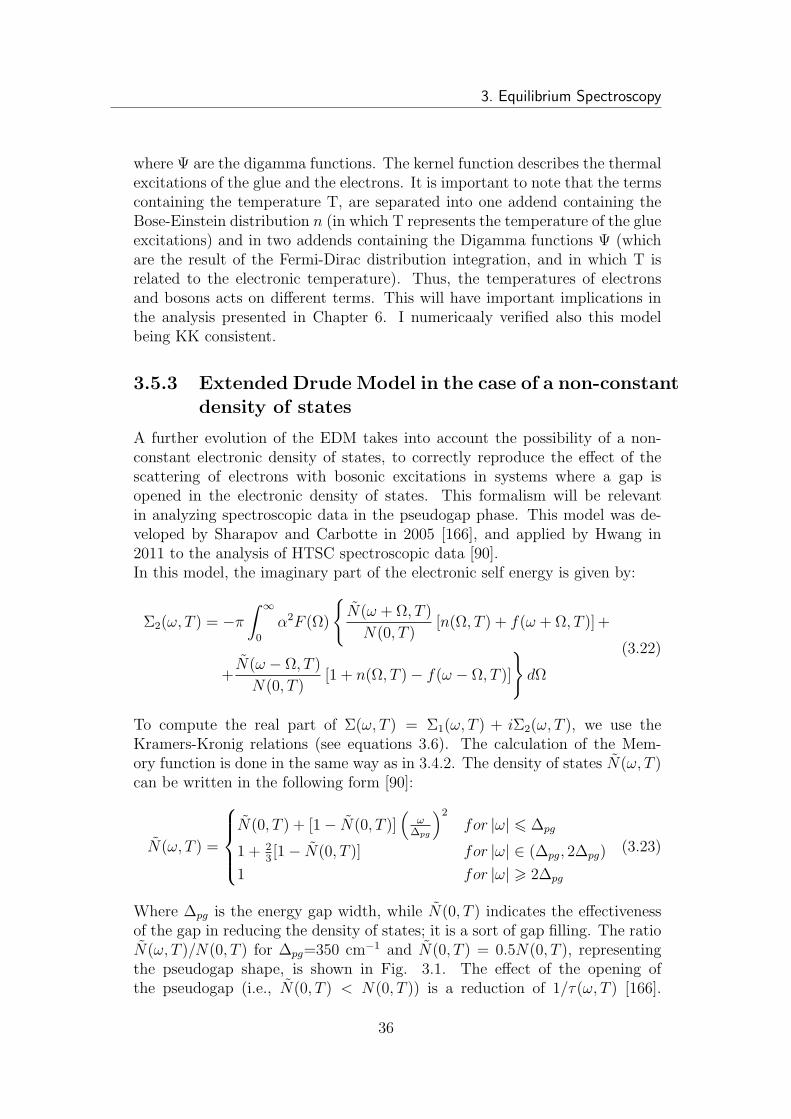
3. Equilibrium Spectroscopy
where Ψ are the digamma functions. The kernel function describes the thermalexcitations of the glue and the electrons. It is important to note that the termscontaining the temperature T, are separated into one addend containing theBose-Einstein distribution n (in which T represents the temperature of the glueexcitations) and in two addends containing the Digamma functions Ψ (whichare the result of the Fermi-Dirac distribution integration, and in which T isrelated to the electronic temperature). Thus, the temperatures of electronsand bosons acts on different terms. This will have important implications inthe analysis presented in Chapter 6. I numericaaly verified also this modelbeing KK consistent.
3.5.3 Extended Drude Model in the case of a non-constantdensity of states
A further evolution of the EDM takes into account the possibility of a non-constant electronic density of states, to correctly reproduce the effect of thescattering of electrons with bosonic excitations in systems where a gap isopened in the electronic density of states. This formalism will be relevantin analyzing spectroscopic data in the pseudogap phase. This model was de-veloped by Sharapov and Carbotte in 2005 [166], and applied by Hwang in2011 to the analysis of HTSC spectroscopic data [90].In this model, the imaginary part of the electronic self energy is given by:
Σ2(ω, T ) = −π
∫ ∞
0
α2F (Ω)
N(ω + Ω, T )
N(0, T )[n(Ω, T ) + f(ω + Ω, T )] +
+N(ω − Ω, T )
N(0, T )[1 + n(Ω, T )− f(ω − Ω, T )]
dΩ
(3.22)
To compute the real part of Σ(ω, T ) = Σ1(ω, T ) + iΣ2(ω, T ), we use theKramers-Kronig relations (see equations 3.6). The calculation of the Mem-ory function is done in the same way as in 3.4.2. The density of states N(ω, T )can be written in the following form [90]:
N(ω, T ) =
N(0, T ) + [1− N(0, T )](
ω∆pg
)2
for |ω| 6 ∆pg
1 + 23[1− N(0, T )] for |ω| ∈ (∆pg, 2∆pg)
1 for |ω| > 2∆pg
(3.23)
Where ∆pg is the energy gap width, while N(0, T ) indicates the effectivenessof the gap in reducing the density of states; it is a sort of gap filling. The ratioN(ω, T )/N(0, T ) for ∆pg=350 cm−1 and N(0, T ) = 0.5N(0, T ), representingthe pseudogap shape, is shown in Fig. 3.1. The effect of the opening ofthe pseudogap (i.e., N(0, T ) < N(0, T )) is a reduction of 1/τ(ω, T ) [166].
36
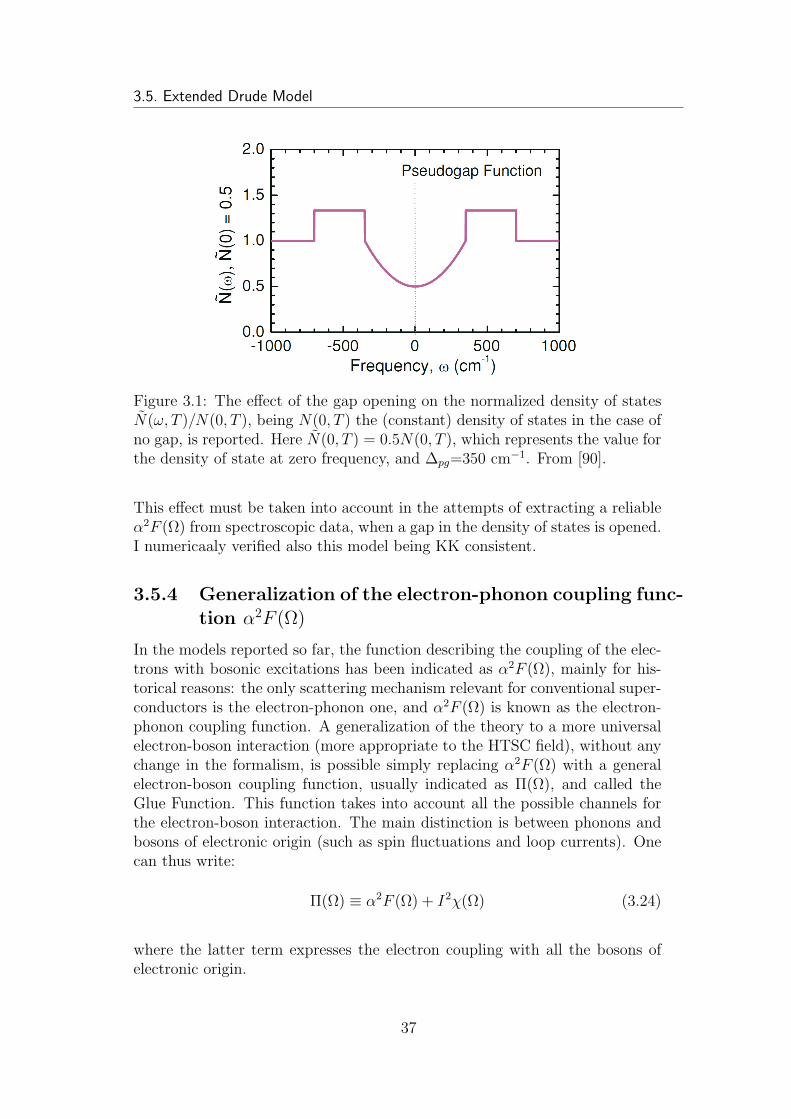
3.5. Extended Drude Model
Figure 3.1: The effect of the gap opening on the normalized density of statesN(ω, T )/N(0, T ), being N(0, T ) the (constant) density of states in the case ofno gap, is reported. Here N(0, T ) = 0.5N(0, T ), which represents the value forthe density of state at zero frequency, and ∆pg=350 cm−1. From [90].
This effect must be taken into account in the attempts of extracting a reliableα2F (Ω) from spectroscopic data, when a gap in the density of states is opened.I numericaaly verified also this model being KK consistent.
3.5.4 Generalization of the electron-phonon coupling func-tion α2F (Ω)
In the models reported so far, the function describing the coupling of the elec-trons with bosonic excitations has been indicated as α2F (Ω), mainly for his-torical reasons: the only scattering mechanism relevant for conventional super-conductors is the electron-phonon one, and α2F (Ω) is known as the electron-phonon coupling function. A generalization of the theory to a more universalelectron-boson interaction (more appropriate to the HTSC field), without anychange in the formalism, is possible simply replacing α2F (Ω) with a generalelectron-boson coupling function, usually indicated as Π(Ω), and called theGlue Function. This function takes into account all the possible channels forthe electron-boson interaction. The main distinction is between phonons andbosons of electronic origin (such as spin fluctuations and loop currents). Onecan thus write:
Π(Ω) ≡ α2F (Ω) + I2χ(Ω) (3.24)
where the latter term expresses the electron coupling with all the bosons ofelectronic origin.
37
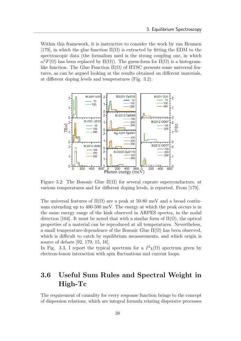
3. Equilibrium Spectroscopy
Within this framework, it is instructive to consider the work by van Heumen[179], in which the glue function Π(Ω) is extracted by fitting the EDM to thespectroscopic data (the formalism used is the strong coupling one, in whichα2F (Ω) has been replaced by Π(Ω)). The guess-form for Π(Ω) is a histogram-like function. The Glue Function Π(Ω) of HTSC presents some universal fea-tures, as can be argued looking at the results obtained on different materials,at different doping levels and temperatures (Fig. 3.2).
Figure 3.2: The Bosonic Glue Π(Ω) for several cuprate superconductors, atvarious temperatures and for different doping levels, is reported. From [179].
The universal features of Π(Ω) are a peak at 50-80 meV and a broad contin-uum extending up to 400-500 meV. The energy at which the peak occurs is inthe same energy range of the kink observed in ARPES spectra, in the nodaldirection [104]. It must be noted that with a similar form of Π(Ω), the opticalproperties of a material can be reproduced at all temperatures. Nevertheless,a small temperature-dependence of the Bosonic Glue Π(Ω) has been observed,which is difficult to catch by equilibrium measurements, and which origin issource of debate [92, 179, 15, 16].In Fig. 3.3, I report the typical spectrum for a I2χ(Ω) spectrum given byelectron-boson interaction with spin fluctuations and current loops.
3.6 Useful Sum Rules and Spectral Weight in
High-Tc
The requirement of causality for every response function brings to the conceptof dispersion relations, which are integral formula relating dispersive processes
38
3.6. Useful Sum Rules and Spectral Weight in High-Tc
Figure 3.3: a) A typical I2χ(Ω) spectrum for spin fluctuations, measured byinelastic neutron scattering on a YBCO sample, is reported. From [47]. b)A typical I2χ(Ω) spectrum (here labeled as Eliashberg coupling function) forthe magnetic excitation modes of the current loop ground state is reported. Itis extracted from ARPES data on a slightly under-doped Bi2212 compound.The angle indicates the direction of the cut in the Brillouin zone along whichdata are extracted; it is measured from the Y Γ direction. From [34].
to absorption ones (causality requires that absorption and dispersion processesbe intimately related, and cannot be considered as independent). The realand imaginary parts of the dielectric function ǫ(ω) or of the refraction indexn(ω) are thus related by a dispersion relation, expressed through the Kramers-Kronig integral relations. However, these relations hold for the real and theimaginary parts of any response function (see equations 3.6).Starting from these relations, it is possible to derive useful sum rules, the mostimportant of which is the so-called f -sum rule (or global oscillator strengthsum rule):
∫ ∞
0
ωǫ2(ω)dω =π
2ω2p (3.25)
where ωp is the dressed plasma frequency of the system, i.e.: ωp2 = 4πNe2
m,
being N the total density of electrons participating to the interaction with theelectromagnetic wave.Sum rules indicate conserved quantities, that is, quantities that do no changeunder a change, for example, of temperature. Analyzing the left hand side ofeq. 3.n, it turns out that N must be a conserved quantity.From this sum rule, the concept of spectral weight (SW) follows straightfor-wardly: It is defined by:
SW ≡∫ ∞
0
σ1(ω)dω =1
8ω2p (3.26)
SW is by definition a conserved quantity.
39
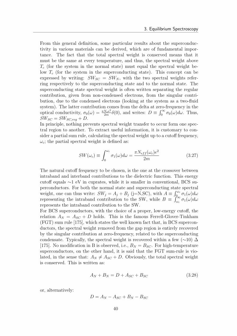
3. Equilibrium Spectroscopy
From this general definition, some particular results about the superconduc-tivity in various materials can be derived, which are of fundamental impor-tance. The fact that the total spectral weight is conserved means that itmust be the same at every temperature, and thus, the spectral weight aboveTc (for the system in the normal state) must equal the spectral weight be-low Tc (for the system in the superconducting state). This concept can beexpressed by writing: SWSC = SWN , with the two spectral weights refer-ring respectively to the superconducting state and to the normal state. Thesuperconducting state spectral weight is often written separating the regularcontribution, given from non-condensed electrons, from the singular contri-bution, due to the condensed electrons (looking at the system as a two-fluidsystem). The latter contribution comes from the delta at zero-frequency in theoptical conductivity, σ0(ω) =
πNse2
2mδ(0), and writes: D ≡
∫∞
0σ0(ω)dω. Thus,
SWSC = SWSC,reg +D.In principle, nothing prevents spectral weight transfer to occur form one spec-tral region to another. To extract useful information, it is customary to con-sider a partial sum rule, calculating the spectral weight up to a cutoff frequency,ωc; the partial spectral weight is defined as:
SW (ωc) ≡∫ ωc
0
σ1(ω)dω =πNeff (ωc)e
2
2m(3.27)
The natural cutoff frequency to be chosen, is the one at the crossover betweenintraband and interband contributions to the dielectric function. This energycutoff equals ∼1 eV in cuprates, while it is smaller in conventional, BCS su-perconductors. For both the normal state and superconducting state spectralweight, one can thus write: SWj = Aj + Bj (j=N,SC), with A ≡
∫ ωc
0σ1(ω)dω
representing the intraband contribution to the SW, while B ≡∫∞
ωcσ1(ω)dω
represents the intraband contribution to the SW.For BCS superconductors, with the choice of a proper, low-energy cutoff, therelation AN = ASC + D holds. This is the famous Ferrell-Glover-Tinkham(FGT) sum rule [175], which states the well known fact that, in BCS supercon-ductors, the spectral weight removed from the gap region is entirely recoveredby the singular contribution at zero-frequency, related to the superconductingcondensate. Typically, the spectral weight is recovered within a few (∼10) ∆[175]. No modification in B is observed, i.e., BN = BSC . For high-temperaturesuperconductors, on the other hand, it is said that the FGT sum-rule is vio-lated, in the sense that: AN 6= ASC +D. Obviously, the total spectral weightis conserved. This is written as:
AN + BN = D + ASC + BSC (3.28)
or, alternatively:
D = AN − ASC + BN − BSC
40
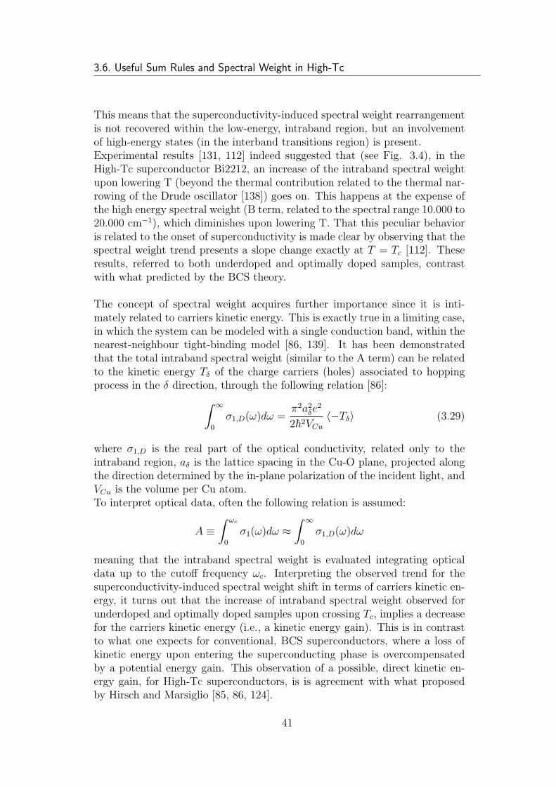
3.6. Useful Sum Rules and Spectral Weight in High-Tc
This means that the superconductivity-induced spectral weight rearrangementis not recovered within the low-energy, intraband region, but an involvementof high-energy states (in the interband transitions region) is present.Experimental results [131, 112] indeed suggested that (see Fig. 3.4), in theHigh-Tc superconductor Bi2212, an increase of the intraband spectral weightupon lowering T (beyond the thermal contribution related to the thermal nar-rowing of the Drude oscillator [138]) goes on. This happens at the expense ofthe high energy spectral weight (B term, related to the spectral range 10.000 to20.000 cm−1), which diminishes upon lowering T. That this peculiar behavioris related to the onset of superconductivity is made clear by observing that thespectral weight trend presents a slope change exactly at T = Tc [112]. Theseresults, referred to both underdoped and optimally doped samples, contrastwith what predicted by the BCS theory.
The concept of spectral weight acquires further importance since it is inti-mately related to carriers kinetic energy. This is exactly true in a limiting case,in which the system can be modeled with a single conduction band, within thenearest-neighbour tight-binding model [86, 139]. It has been demonstratedthat the total intraband spectral weight (similar to the A term) can be relatedto the kinetic energy Tδ of the charge carriers (holes) associated to hoppingprocess in the δ direction, through the following relation [86]:
∫ ∞
0
σ1,D(ω)dω =π2a2δe
2
2~2VCu
〈−Tδ〉 (3.29)
where σ1,D is the real part of the optical conductivity, related only to theintraband region, aδ is the lattice spacing in the Cu-O plane, projected alongthe direction determined by the in-plane polarization of the incident light, andVCu is the volume per Cu atom.To interpret optical data, often the following relation is assumed:
A ≡∫ ωc
0
σ1(ω)dω ≈∫ ∞
0
σ1,D(ω)dω
meaning that the intraband spectral weight is evaluated integrating opticaldata up to the cutoff frequency ωc. Interpreting the observed trend for thesuperconductivity-induced spectral weight shift in terms of carriers kinetic en-ergy, it turns out that the increase of intraband spectral weight observed forunderdoped and optimally doped samples upon crossing Tc, implies a decreasefor the carriers kinetic energy (i.e., a kinetic energy gain). This is in contrastto what one expects for conventional, BCS superconductors, where a loss ofkinetic energy upon entering the superconducting phase is overcompensatedby a potential energy gain. This observation of a possible, direct kinetic en-ergy gain, for High-Tc superconductors, is is agreement with what proposedby Hirsch and Marsiglio [85, 86, 124].
41
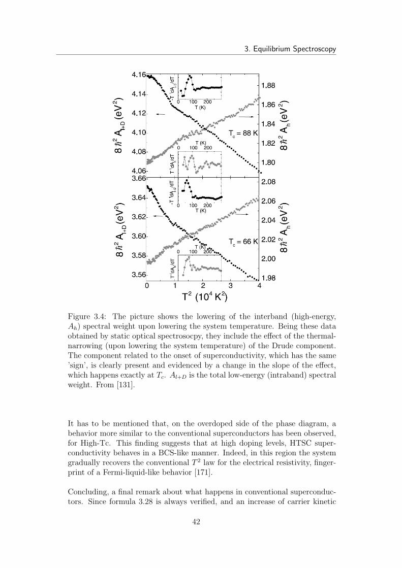
3. Equilibrium Spectroscopy
Figure 3.4: The picture shows the lowering of the interband (high-energy,Ah) spectral weight upon lowering the system temperature. Being these dataobtained by static optical spectrosocpy, they include the effect of the thermal-narrowing (upon lowering the system temperature) of the Drude component.The component related to the onset of superconductivity, which has the same’sign’, is clearly present and evidenced by a change in the slope of the effect,which happens exactly at Tc. Al+D is the total low-energy (intraband) spectralweight. From [131].
It has to be mentioned that, on the overdoped side of the phase diagram, abehavior more similar to the conventional superconductors has been observed,for High-Tc. This finding suggests that at high doping levels, HTSC super-conductivity behaves in a BCS-like manner. Indeed, in this region the systemgradually recovers the conventional T 2 law for the electrical resistivity, finger-print of a Fermi-liquid-like behavior [171].
Concluding, a final remark about what happens in conventional superconduc-tors. Since formula 3.28 is always verified, and an increase of carrier kinetic
42
3.7. Y-Bi2212 Static Dielectric Functions Analysis
energy upon lowering temperature below Tc directly follows from BCS the-ory, a slight transfer of spectral weight to high energies must happen. Thus,though experimentally undetectable, a small spectral weight transfer must ex-ist (a spectral weight transfer has never been observed in BCS superconductors,since it is proportional to the condensation energy [175], in tuurn proportionalto ∆2, which in BCS systems is of the order ∼1 meV [175]). In a certainsense, the FGT sum rule is strictly never true. FGT sum rule is indeed aphenomenological relation, and up to now no such spectral weight transfer hasbeen measured in conventional superconductors.
From equilibrium optical measurement, with the help of the illustrated sumrule, very important informations about the mechanisms driving the supercon-ducting transition in copper oxide based superconductors have been extracted[131, 179, 139, 138]. Anyway, these findings are not conclusive, in the senseof assigning these spectral weight shifts a clear physical origin. Moreover,the problem of the thermal narrowing of the Drude peak, upon lowering thetemperature, must be faced. Recently it has been demonstrated [138] that thetemperature dependence of the optical integral A ≡
∫ ωc
0σ1(ω)dω in the normal
state of the cuprates is due solely to a cutoff-dependent term that accounts forthe extension of the Drude peak beyond the upper bound ωc of the integral,rather than to a true sum-rule violation. This implies that the dominant con-tribution to the observed sum-rule violation in the normal state is only due tothe finite cutoff ωc and to a thermal effect.With the help of the recently developed time-resolved spectroscopic technique(see Chapter 5), we were able to clarify that the whole spectral weight trans-fer observed by static spectroscopies upon entering the superconducting phasecomes precisely from two high energy states (at 1.5 and 2 eV), and that a trendform a superconductivity induced kinetic energy gain in the underdoped sideof the phase diagram, to a BCS-like superconductivity induced kinetic energyloss in the overdoped side of the phase diagram, exists. More details can befound in Chapter 8. The time-resolution eliminates the problem of the finitecutoff ωc, being the electronic effects related to the condensate formation andthe thermal ones disentangled by their timescales.
3.7 Y-Bi2212 Static Dielectric Functions Anal-
ysis
In this conclusive paragraph I present the results of the fitting of the Lorentzand Extended Drude model dielectric function, with the proper formalism, tothe optimally doped Y-Bi2212 sample (Tc=96 K) dielectric function experi-mental data. I will treat singularly the cases of the optical properties for theY-Bi2212 sample in the normal state phase (T=300 K, section 3.7.1), in thepseudogap phase (T=100 K, section 3.7.2) and in the superconducting phase
43
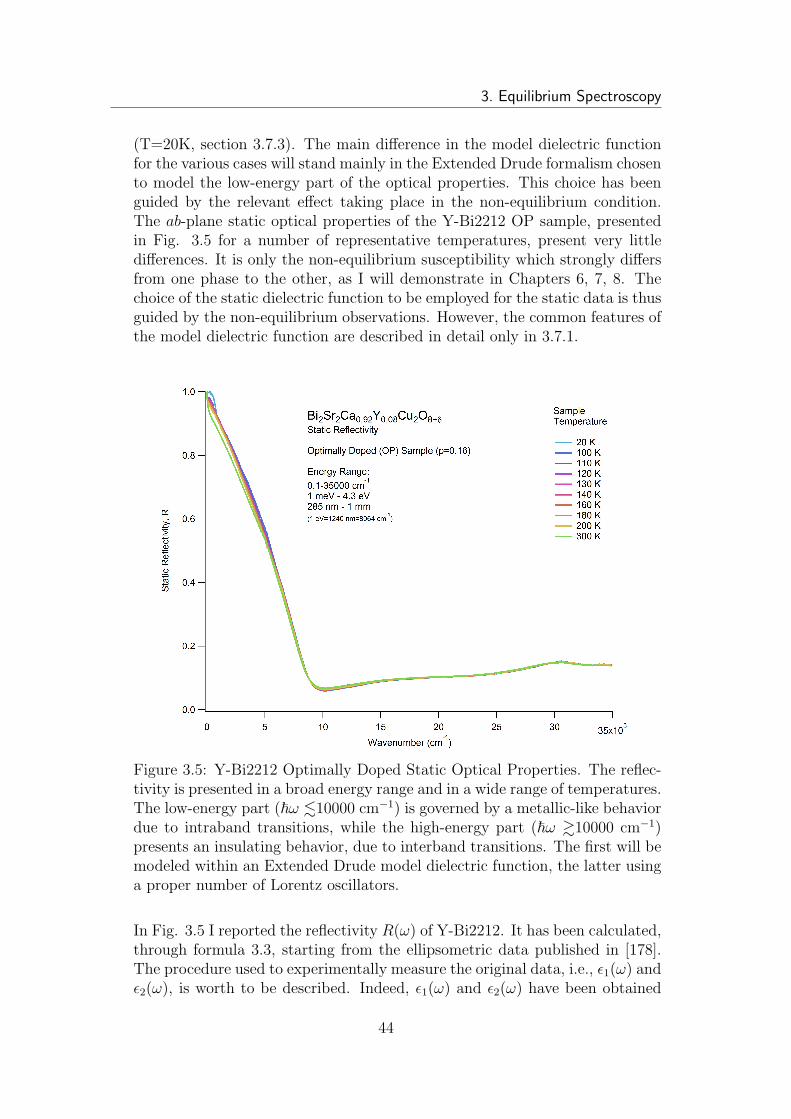
3. Equilibrium Spectroscopy
(T=20K, section 3.7.3). The main difference in the model dielectric functionfor the various cases will stand mainly in the Extended Drude formalism chosento model the low-energy part of the optical properties. This choice has beenguided by the relevant effect taking place in the non-equilibrium condition.The ab-plane static optical properties of the Y-Bi2212 OP sample, presentedin Fig. 3.5 for a number of representative temperatures, present very littledifferences. It is only the non-equilibrium susceptibility which strongly differsfrom one phase to the other, as I will demonstrate in Chapters 6, 7, 8. Thechoice of the static dielectric function to be employed for the static data is thusguided by the non-equilibrium observations. However, the common features ofthe model dielectric function are described in detail only in 3.7.1.
Figure 3.5: Y-Bi2212 Optimally Doped Static Optical Properties. The reflec-tivity is presented in a broad energy range and in a wide range of temperatures.The low-energy part (~ω .10000 cm−1) is governed by a metallic-like behaviordue to intraband transitions, while the high-energy part (~ω &10000 cm−1)presents an insulating behavior, due to interband transitions. The first will bemodeled within an Extended Drude model dielectric function, the latter usinga proper number of Lorentz oscillators.
In Fig. 3.5 I reported the reflectivity R(ω) of Y-Bi2212. It has been calculated,through formula 3.3, starting from the ellipsometric data published in [178].The procedure used to experimentally measure the original data, i.e., ǫ1(ω) andǫ2(ω), is worth to be described. Indeed, ǫ1(ω) and ǫ2(ω) have been obtained
44
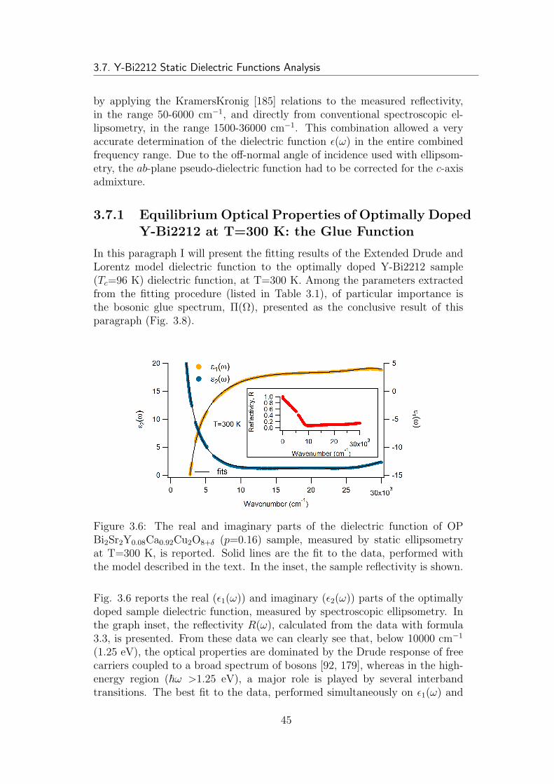
3.7. Y-Bi2212 Static Dielectric Functions Analysis
by applying the KramersKronig [185] relations to the measured reflectivity,in the range 50-6000 cm−1, and directly from conventional spectroscopic el-lipsometry, in the range 1500-36000 cm−1. This combination allowed a veryaccurate determination of the dielectric function ǫ(ω) in the entire combinedfrequency range. Due to the off-normal angle of incidence used with ellipsom-etry, the ab-plane pseudo-dielectric function had to be corrected for the c-axisadmixture.
3.7.1 Equilibrium Optical Properties of Optimally DopedY-Bi2212 at T=300 K: the Glue Function
In this paragraph I will present the fitting results of the Extended Drude andLorentz model dielectric function to the optimally doped Y-Bi2212 sample(Tc=96 K) dielectric function, at T=300 K. Among the parameters extractedfrom the fitting procedure (listed in Table 3.1), of particular importance isthe bosonic glue spectrum, Π(Ω), presented as the conclusive result of thisparagraph (Fig. 3.8).
Figure 3.6: The real and imaginary parts of the dielectric function of OPBi2Sr2Y0.08Ca0.92Cu2O8+δ (p=0.16) sample, measured by static ellipsometryat T=300 K, is reported. Solid lines are the fit to the data, performed withthe model described in the text. In the inset, the sample reflectivity is shown.
Fig. 3.6 reports the real (ǫ1(ω)) and imaginary (ǫ2(ω)) parts of the optimallydoped sample dielectric function, measured by spectroscopic ellipsometry. Inthe graph inset, the reflectivity R(ω), calculated from the data with formula3.3, is presented. From these data we can clearly see that, below 10000 cm−1
(1.25 eV), the optical properties are dominated by the Drude response of freecarriers coupled to a broad spectrum of bosons [92, 179], whereas in the high-energy region (~ω >1.25 eV), a major role is played by several interbandtransitions. The best fit to the data, performed simultaneously on ǫ1(ω) and
45
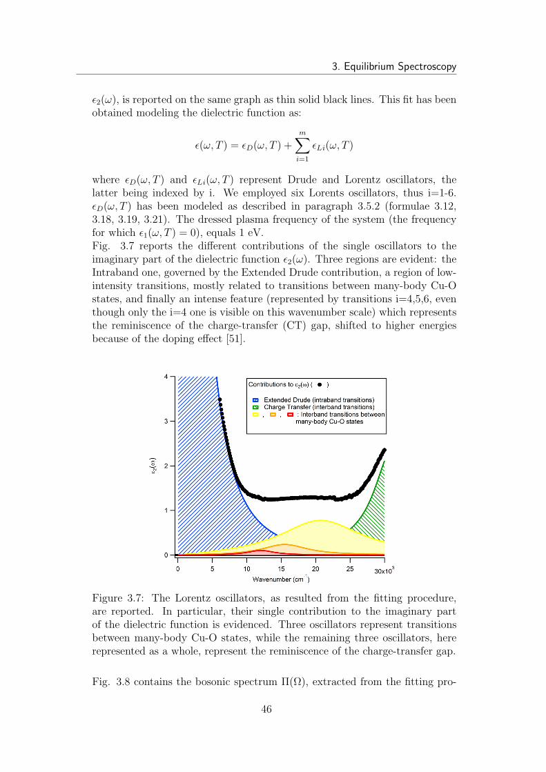
3. Equilibrium Spectroscopy
ǫ2(ω), is reported on the same graph as thin solid black lines. This fit has beenobtained modeling the dielectric function as:
ǫ(ω, T ) = ǫD(ω, T ) +m∑
i=1
ǫLi(ω, T )
where ǫD(ω, T ) and ǫLi(ω, T ) represent Drude and Lorentz oscillators, thelatter being indexed by i. We employed six Lorents oscillators, thus i=1-6.ǫD(ω, T ) has been modeled as described in paragraph 3.5.2 (formulae 3.12,3.18, 3.19, 3.21). The dressed plasma frequency of the system (the frequencyfor which ǫ1(ω, T ) = 0), equals 1 eV.Fig. 3.7 reports the different contributions of the single oscillators to theimaginary part of the dielectric function ǫ2(ω). Three regions are evident: theIntraband one, governed by the Extended Drude contribution, a region of low-intensity transitions, mostly related to transitions between many-body Cu-Ostates, and finally an intense feature (represented by transitions i=4,5,6, eventhough only the i=4 one is visible on this wavenumber scale) which representsthe reminiscence of the charge-transfer (CT) gap, shifted to higher energiesbecause of the doping effect [51].
Figure 3.7: The Lorentz oscillators, as resulted from the fitting procedure,are reported. In particular, their single contribution to the imaginary partof the dielectric function is evidenced. Three oscillators represent transitionsbetween many-body Cu-O states, while the remaining three oscillators, hererepresented as a whole, represent the reminiscence of the charge-transfer gap.
Fig. 3.8 contains the bosonic spectrum Π(Ω), extracted from the fitting pro-
46
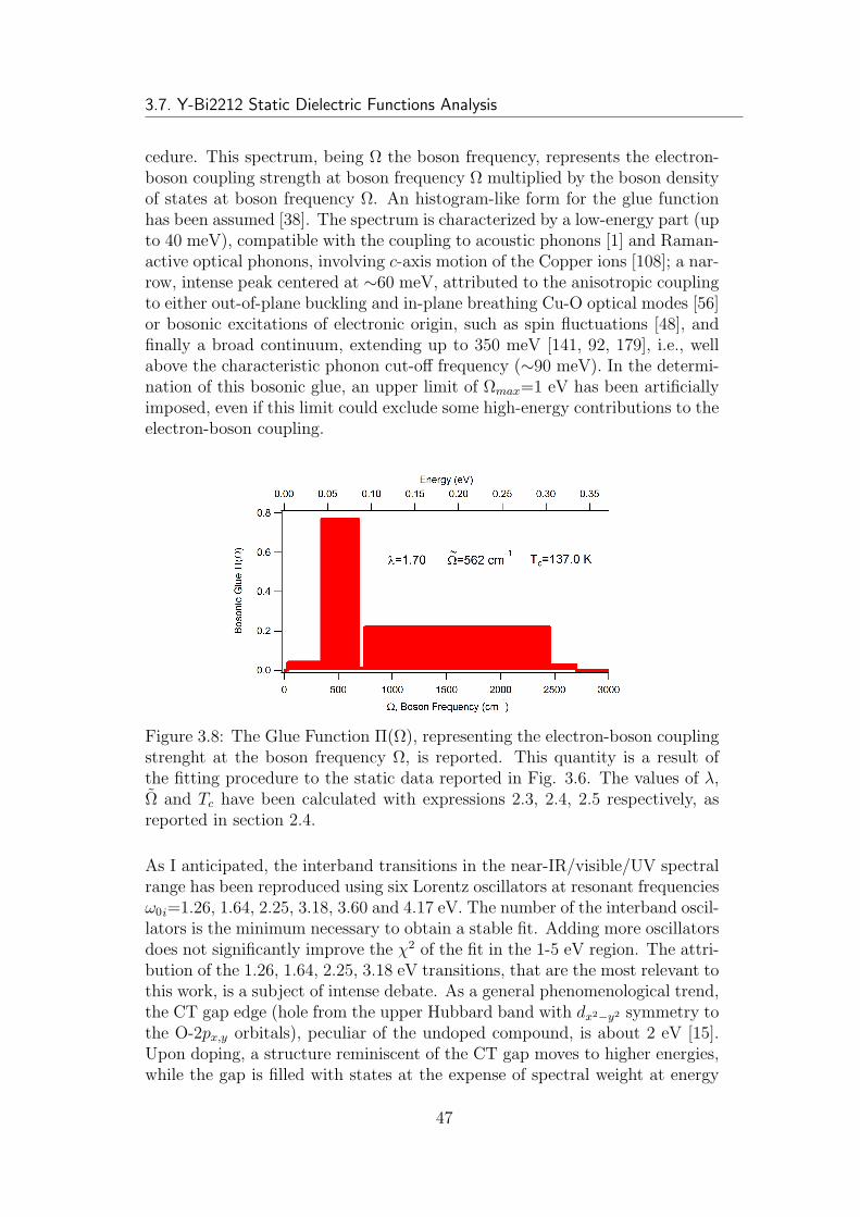
3.7. Y-Bi2212 Static Dielectric Functions Analysis
cedure. This spectrum, being Ω the boson frequency, represents the electron-boson coupling strength at boson frequency Ω multiplied by the boson densityof states at boson frequency Ω. An histogram-like form for the glue functionhas been assumed [38]. The spectrum is characterized by a low-energy part (upto 40 meV), compatible with the coupling to acoustic phonons [1] and Raman-active optical phonons, involving c-axis motion of the Copper ions [108]; a nar-row, intense peak centered at ∼60 meV, attributed to the anisotropic couplingto either out-of-plane buckling and in-plane breathing Cu-O optical modes [56]or bosonic excitations of electronic origin, such as spin fluctuations [48], andfinally a broad continuum, extending up to 350 meV [141, 92, 179], i.e., wellabove the characteristic phonon cut-off frequency (∼90 meV). In the determi-nation of this bosonic glue, an upper limit of Ωmax=1 eV has been artificiallyimposed, even if this limit could exclude some high-energy contributions to theelectron-boson coupling.
Figure 3.8: The Glue Function Π(Ω), representing the electron-boson couplingstrenght at the boson frequency Ω, is reported. This quantity is a result ofthe fitting procedure to the static data reported in Fig. 3.6. The values of λ,Ω and Tc have been calculated with expressions 2.3, 2.4, 2.5 respectively, asreported in section 2.4.
As I anticipated, the interband transitions in the near-IR/visible/UV spectralrange has been reproduced using six Lorentz oscillators at resonant frequenciesω0i=1.26, 1.64, 2.25, 3.18, 3.60 and 4.17 eV. The number of the interband oscil-lators is the minimum necessary to obtain a stable fit. Adding more oscillatorsdoes not significantly improve the χ2 of the fit in the 1-5 eV region. The attri-bution of the 1.26, 1.64, 2.25, 3.18 eV transitions, that are the most relevant tothis work, is a subject of intense debate. As a general phenomenological trend,the CT gap edge (hole from the upper Hubbard band with dx2−y2 symmetry tothe O-2px,y orbitals), peculiar of the undoped compound, is about 2 eV [15].Upon doping, a structure reminiscent of the CT gap moves to higher energies,while the gap is filled with states at the expense of spectral weight at energy
47
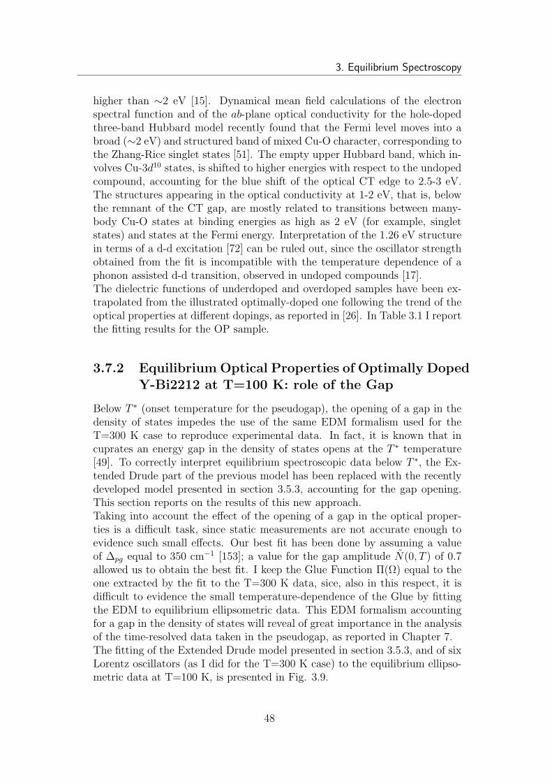
3. Equilibrium Spectroscopy
higher than ∼2 eV [15]. Dynamical mean field calculations of the electronspectral function and of the ab-plane optical conductivity for the hole-dopedthree-band Hubbard model recently found that the Fermi level moves into abroad (∼2 eV) and structured band of mixed Cu-O character, corresponding tothe Zhang-Rice singlet states [51]. The empty upper Hubbard band, which in-volves Cu-3d10 states, is shifted to higher energies with respect to the undopedcompound, accounting for the blue shift of the optical CT edge to 2.5-3 eV.The structures appearing in the optical conductivity at 1-2 eV, that is, belowthe remnant of the CT gap, are mostly related to transitions between many-body Cu-O states at binding energies as high as 2 eV (for example, singletstates) and states at the Fermi energy. Interpretation of the 1.26 eV structurein terms of a d-d excitation [72] can be ruled out, since the oscillator strengthobtained from the fit is incompatible with the temperature dependence of aphonon assisted d-d transition, observed in undoped compounds [17].The dielectric functions of underdoped and overdoped samples have been ex-trapolated from the illustrated optimally-doped one following the trend of theoptical properties at different dopings, as reported in [26]. In Table 3.1 I reportthe fitting results for the OP sample.
3.7.2 Equilibrium Optical Properties of Optimally DopedY-Bi2212 at T=100 K: role of the Gap
Below T ∗ (onset temperature for the pseudogap), the opening of a gap in thedensity of states impedes the use of the same EDM formalism used for theT=300 K case to reproduce experimental data. In fact, it is known that incuprates an energy gap in the density of states opens at the T ∗ temperature[49]. To correctly interpret equilibrium spectroscopic data below T ∗, the Ex-tended Drude part of the previous model has been replaced with the recentlydeveloped model presented in section 3.5.3, accounting for the gap opening.This section reports on the results of this new approach.Taking into account the effect of the opening of a gap in the optical proper-ties is a difficult task, since static measurements are not accurate enough toevidence such small effects. Our best fit has been done by assuming a valueof ∆pg equal to 350 cm−1 [153]; a value for the gap amplitude N(0, T ) of 0.7allowed us to obtain the best fit. I keep the Glue Function Π(Ω) equal to theone extracted by the fit to the T=300 K data, sice, also in this respect, it isdifficult to evidence the small temperature-dependence of the Glue by fittingthe EDM to equilibrium ellipsometric data. This EDM formalism accountingfor a gap in the density of states will reveal of great importance in the analysisof the time-resolved data taken in the pseudogap, as reported in Chapter 7.The fitting of the Extended Drude model presented in section 3.5.3, and of sixLorentz oscillators (as I did for the T=300 K case) to the equilibrium ellipso-metric data at T=100 K, is presented in Fig. 3.9.
48
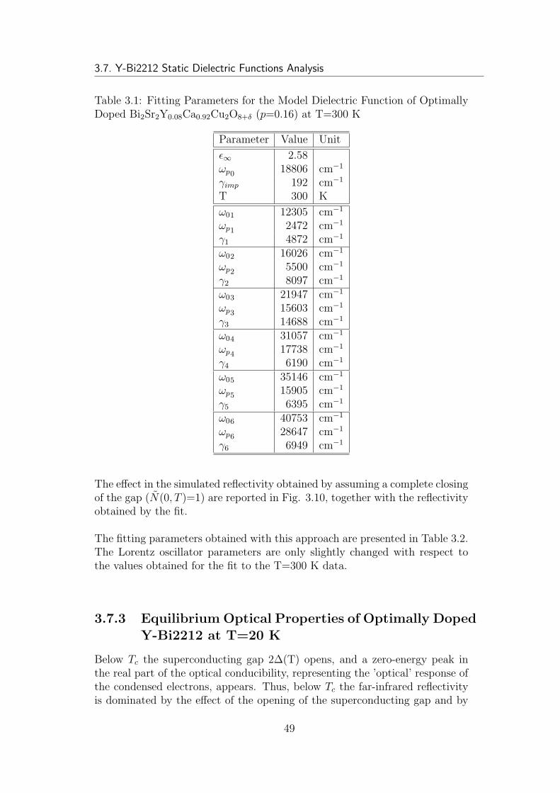
3.7. Y-Bi2212 Static Dielectric Functions Analysis
Table 3.1: Fitting Parameters for the Model Dielectric Function of OptimallyDoped Bi2Sr2Y0.08Ca0.92Cu2O8+δ (p=0.16) at T=300 K
Parameter Value Unit
ǫ∞ 2.58ωp0 18806 cm−1
γimp 192 cm−1
T 300 K
ω01 12305 cm−1
ωp1 2472 cm−1
γ1 4872 cm−1
ω02 16026 cm−1
ωp2 5500 cm−1
γ2 8097 cm−1
ω03 21947 cm−1
ωp3 15603 cm−1
γ3 14688 cm−1
ω04 31057 cm−1
ωp4 17738 cm−1
γ4 6190 cm−1
ω05 35146 cm−1
ωp5 15905 cm−1
γ5 6395 cm−1
ω06 40753 cm−1
ωp6 28647 cm−1
γ6 6949 cm−1
The effect in the simulated reflectivity obtained by assuming a complete closingof the gap (N(0, T )=1) are reported in Fig. 3.10, together with the reflectivityobtained by the fit.
The fitting parameters obtained with this approach are presented in Table 3.2.The Lorentz oscillator parameters are only slightly changed with respect tothe values obtained for the fit to the T=300 K data.
3.7.3 Equilibrium Optical Properties of Optimally DopedY-Bi2212 at T=20 K
Below Tc the superconducting gap 2∆(T) opens, and a zero-energy peak inthe real part of the optical conducibility, representing the ’optical’ response ofthe condensed electrons, appears. Thus, below Tc the far-infrared reflectivityis dominated by the effect of the opening of the superconducting gap and by
49
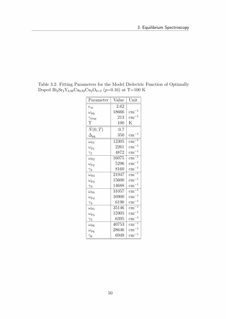
3. Equilibrium Spectroscopy
Table 3.2: Fitting Parameters for the Model Dielectric Function of OptimallyDoped Bi2Sr2Y0.08Ca0.92Cu2O8+δ (p=0.16) at T=100 K
Parameter Value Unit
ǫ∞ 2.62ωp0 18666 cm−1
γimp 213 cm−1
T 100 K
N(0, T ) 0.7∆pg 350 cm−1
ω01 12305 cm−1
ωp1 2261 cm−1
γ1 4872 cm−1
ω02 16075 cm−1
ωp2 5296 cm−1
γ2 8160 cm−1
ω03 21947 cm−1
ωp3 15600 cm−1
γ3 14688 cm−1
ω04 31057 cm−1
ωp4 16900 cm−1
γ4 6190 cm−1
ω05 35146 cm−1
ωp5 15905 cm−1
γ5 6395 cm−1
ω06 40753 cm−1
ωp6 28646 cm−1
γ6 6949 cm−1
50
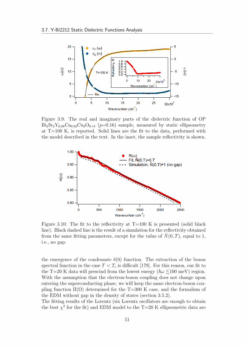
3.7. Y-Bi2212 Static Dielectric Functions Analysis
Figure 3.9: The real and imaginary parts of the dielectric function of OPBi2Sr2Y0.08Ca0.92Cu2O8+δ (p=0.16) sample, measured by static ellipsometryat T=100 K, is reported. Solid lines are the fit to the data, performed withthe model described in the text. In the inset, the sample reflectivity is shown.
Figure 3.10: The fit to the reflectivity at T=100 K is presented (solid blackline). Black dashed line is the result of a simulation for the reflectivity obtainedfrom the same fitting parameters, except for the value of N(0, T ), equal to 1,i.e., no gap.
the emergence of the condensate δ(0) function. The extraction of the bosonspectral function in the case T < Tc is difficult [179]. For this reason, our fit tothe T=20 K data will prescind from the lowest energy (~ω .100 meV) region.With the assumption that the electron-boson coupling does not change uponentering the superconducting phase, we will keep the same electron-boson cou-pling function Π(Ω) determined for the T=300 K case, and the formalism ofthe EDM without gap in the density of states (section 3.5.2).The fitting results of the Lorentz (six Lorentz oscillators are enough to obtainthe best χ2 for the fit) and EDM model to the T=20 K ellipsometric data are
51
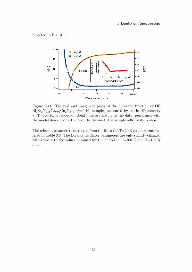
3. Equilibrium Spectroscopy
reported in Fig. 3.11.
Figure 3.11: The real and imaginary parts of the dielectric function of OPBi2Sr2Y0.08Ca0.92Cu2O8+δ (p=0.16) sample, measured by static ellipsometryat T=100 K, is reported. Solid lines are the fit to the data, performed withthe model described in the text. In the inset, the sample reflectivity is shown.
The relevant parameters extracted from the fit to the T=20 K data are summa-rized in Table 3.3. The Lorentz oscillator parameters are only slightly changedwith respect to the values obtained for the fit to the T=300 K and T=100 Kdata.
52
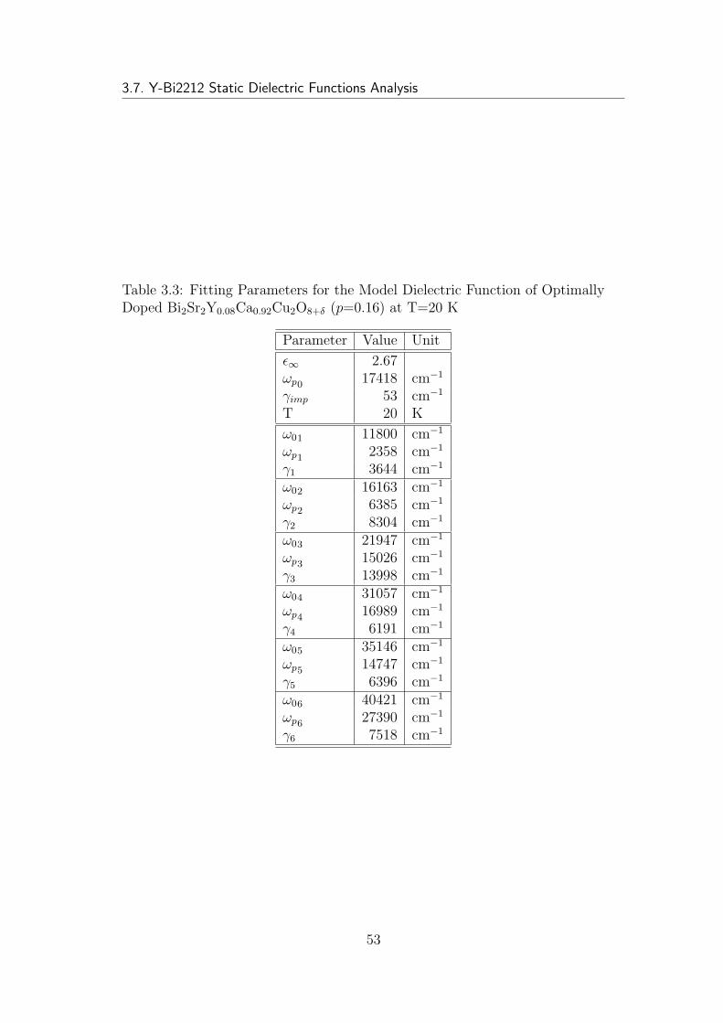
3.7. Y-Bi2212 Static Dielectric Functions Analysis
Table 3.3: Fitting Parameters for the Model Dielectric Function of OptimallyDoped Bi2Sr2Y0.08Ca0.92Cu2O8+δ (p=0.16) at T=20 K
Parameter Value Unit
ǫ∞ 2.67ωp0 17418 cm−1
γimp 53 cm−1
T 20 K
ω01 11800 cm−1
ωp1 2358 cm−1
γ1 3644 cm−1
ω02 16163 cm−1
ωp2 6385 cm−1
γ2 8304 cm−1
ω03 21947 cm−1
ωp3 15026 cm−1
γ3 13998 cm−1
ω04 31057 cm−1
ωp4 16989 cm−1
γ4 6191 cm−1
ω05 35146 cm−1
ωp5 14747 cm−1
γ5 6396 cm−1
ω06 40421 cm−1
ωp6 27390 cm−1
γ6 7518 cm−1
53
3. Equilibrium Spectroscopy
54
Chapter 4Non-Equilibrium Physics ofHTSC
4.1 Introduction
With this chapter I want to underline the importance of non-equilibriumphysics, in understanding some aspects which equilibrium physics cannot prop-erly address. In particular, emphasis will be directed to the information whichcan be gained from non-equilibrium, all-optical time-resolved measurements,based on ultrashort (∼100 fs) laser pulses.In the field of strongly correlated systems, the non-equilibrium physics canshed light on aspects which at equilibrium are masked and entangled, reveal-ing the true nature of the physical phases. This is achieved thanks to boththe temporal resolution of non-equilibrium techniques (which allows to accessto the time domain, in which different kinds of excitations are disentangled bytheir temporal dynamics) and the spectral resolution we have added (whichallows to access to the energy domain, in which the different effects are dis-entangled by their out-of-equilibrium spectral fingerprint). A phase of mattercan be characterized thanks to the knowledge of its own intrinsic susceptibility,i.e., its response to a light-induced perturbation, which can be ascribed eitherto thermal effects, or excited state absorptions, or linear modification of thestatic dielectric function. These different scenarios can indeed be revealed bytime-resolved optical measurements with spectral resolution, which are able toreveal the microscopic changes in the electronic structure, which happen ontimescales much faster than those typical of thermal phenomena. The spectralresolution is of paramount importance since it allows to relate a time-resolvedoptical signal in the energy domain to a peculiar modification of the dielectricfunction of the material, depending upon its electronic band structure. It isthe ability of non-equilibrium physics to temporally and spectrally disentanglethermal effects from electronic ones which allowed us to get new insights onthe HTSC physics, revealing the nature of the different phases of the phase
55
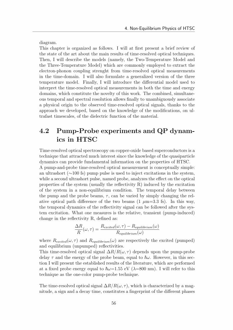
4. Non-Equilibrium Physics of HTSC
diagram.This chapter is organized as follows. I will at first present a brief review ofthe state of the art about the main results of time-resolved optical techniques.Then, I will describe the models (namely, the Two-Temperature Model andthe Three-Temperature Model) which are commonly employed to extract theelectron-phonon coupling strenght from time-resolved optical measurementsin the time-domain. I will also formulate a generalized version of the threetemperature model. Finally, I will introduce the differential model used tointerpret the time-resolved optical measurements in both the time and energydomains, which constitute the novelty of this work. The combined, simultane-ous temporal and spectral rosolution allows finally to unambiguously associatea physical origin to the observed time-resolved optical signals, thanks to theapproach we developed, based on the knowledge of the modifications, on ul-trafast timescales, of the dielectric function of the material.
4.2 Pump-Probe experiments and QP dynam-
ics in HTSC
Time-resolved optical spectroscopy on copper-oxide based superconductors is atechnique that attracted much interest since the knowledge of the quasiparticledynamics can provide fundamental information on the properties of HTSC.A pump-and-probe time-resolved optical measurement is conceptually simple:an ultrashort (∼100 fs) pump pulse is used to inject excitations in the system,while a second ultrashort pulse, named probe, analyzes the effect on the opticalproperties of the system (usually the reflectivity R) induced by the excitationof the system in a non-equilibrium condition. The temporal delay betweenthe pump and the probe beams, τ , can be varied by simply changing the rel-ative optical path difference of the two beams (1 µm=3.3 fs). In this way,the temporal dynamics of the reflectivity signal can be followed after the sys-tem excitation. What one measures is the relative, transient (pump-induced)change in the reflectivity R, defined as:
∆R
R(ω, τ) =
Rexcited(ω, τ)−Requilibrium(ω)
Requilibrium(ω)
where Rexcited(ω, τ) and Requilibrium(ω) are respectively the excited (pumped)and equilibrium (unpumped) reflectivities.This time-resolved optical signal ∆R/R(ω, τ) depends upon the pump-probedelay τ and the energy of the probe beam, equal to ~ω. However, in this sec-tion I will present the established results of the literature, which are performedat a fixed probe energy equal to ~ω=1.55 eV (λ=800 nm). I will refer to thistechnique as the one-color pump-probe technique.
The time-resolved optical signal ∆R/R(ω, τ), which is characterized by a mag-nitude, a sign and a decay time, constitutes a fingerprint of the different phases
56
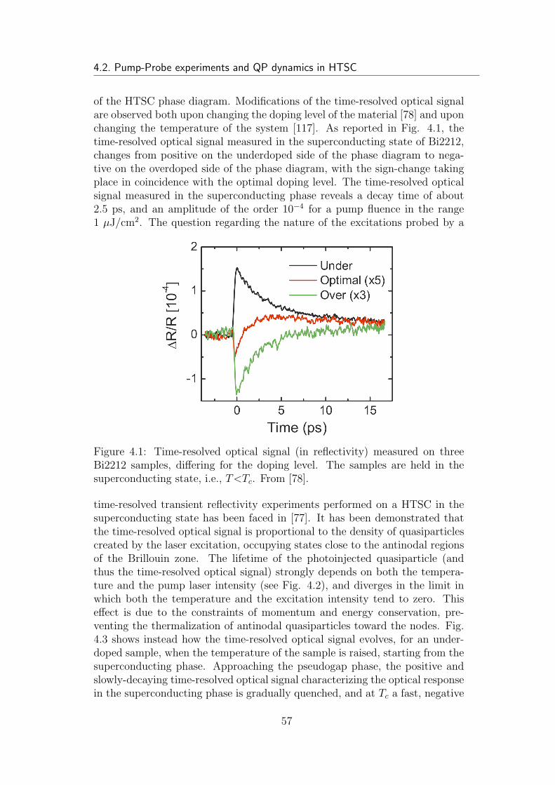
4.2. Pump-Probe experiments and QP dynamics in HTSC
of the HTSC phase diagram. Modifications of the time-resolved optical signalare observed both upon changing the doping level of the material [78] and uponchanging the temperature of the system [117]. As reported in Fig. 4.1, thetime-resolved optical signal measured in the superconducting state of Bi2212,changes from positive on the underdoped side of the phase diagram to nega-tive on the overdoped side of the phase diagram, with the sign-change takingplace in coincidence with the optimal doping level. The time-resolved opticalsignal measured in the superconducting phase reveals a decay time of about2.5 ps, and an amplitude of the order 10−4 for a pump fluence in the range1 µJ/cm2. The question regarding the nature of the excitations probed by a
Figure 4.1: Time-resolved optical signal (in reflectivity) measured on threeBi2212 samples, differing for the doping level. The samples are held in thesuperconducting state, i.e., T<Tc. From [78].
time-resolved transient reflectivity experiments performed on a HTSC in thesuperconducting state has been faced in [77]. It has been demonstrated thatthe time-resolved optical signal is proportional to the density of quasiparticlescreated by the laser excitation, occupying states close to the antinodal regionsof the Brillouin zone. The lifetime of the photoinjected quasiparticle (andthus the time-resolved optical signal) strongly depends on both the tempera-ture and the pump laser intensity (see Fig. 4.2), and diverges in the limit inwhich both the temperature and the excitation intensity tend to zero. Thiseffect is due to the constraints of momentum and energy conservation, pre-venting the thermalization of antinodal quasiparticles toward the nodes. Fig.4.3 shows instead how the time-resolved optical signal evolves, for an under-doped sample, when the temperature of the sample is raised, starting from thesuperconducting phase. Approaching the pseudogap phase, the positive andslowly-decaying time-resolved optical signal characterizing the optical responsein the superconducting phase is gradually quenched, and at Tc a fast, negative
57
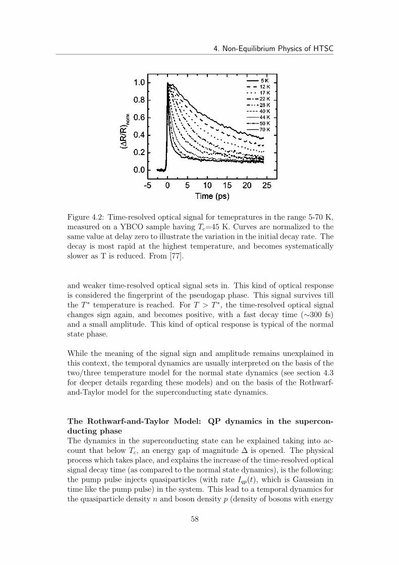
4. Non-Equilibrium Physics of HTSC
Figure 4.2: Time-resolved optical signal for temepratures in the range 5-70 K,measured on a YBCO sample having Tc=45 K. Curves are normalized to thesame value at delay zero to illustrate the variation in the initial decay rate. Thedecay is most rapid at the highest temperature, and becomes systematicallyslower as T is reduced. From [77].
and weaker time-resolved optical signal sets in. This kind of optical responseis considered the fingerprint of the pseudogap phase. This signal survives tillthe T ∗ temperature is reached. For T > T ∗, the time-resolved optical signalchanges sign again, and becomes positive, with a fast decay time (∼300 fs)and a small amplitude. This kind of optical response is typical of the normalstate phase.
While the meaning of the signal sign and amplitude remains unexplained inthis context, the temporal dynamics are usually interpreted on the basis of thetwo/three temperature model for the normal state dynamics (see section 4.3for deeper details regarding these models) and on the basis of the Rothwarf-and-Taylor model for the superconducting state dynamics.
The Rothwarf-and-Taylor Model: QP dynamics in the supercon-ducting phaseThe dynamics in the superconducting state can be explained taking into ac-count that below Tc, an energy gap of magnitude ∆ is opened. The physicalprocess which takes place, and explains the increase of the time-resolved opticalsignal decay time (as compared to the normal state dynamics), is the following:the pump pulse injects quasiparticles (with rate Iqp(t), which is Gaussian intime like the pump pulse) in the system. This lead to a temporal dynamics forthe quasiparticle density n and boson density p (density of bosons with energy
58
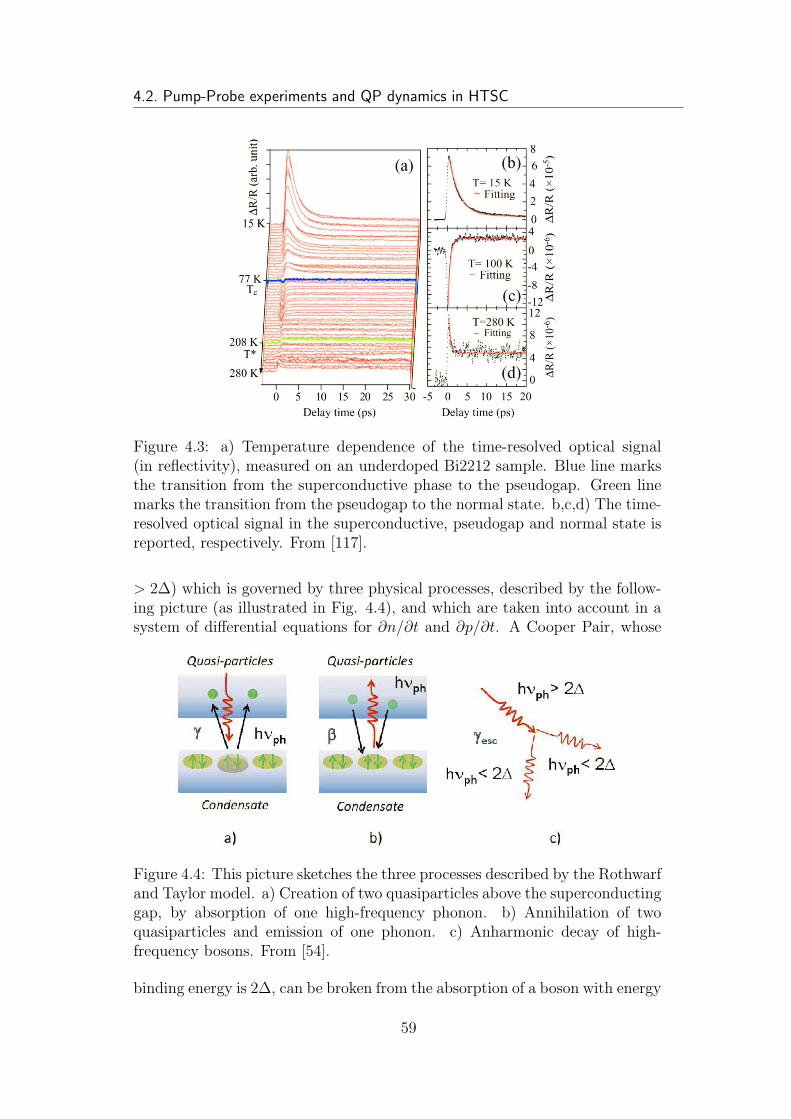
4.2. Pump-Probe experiments and QP dynamics in HTSC
Figure 4.3: a) Temperature dependence of the time-resolved optical signal(in reflectivity), measured on an underdoped Bi2212 sample. Blue line marksthe transition from the superconductive phase to the pseudogap. Green linemarks the transition from the pseudogap to the normal state. b,c,d) The time-resolved optical signal in the superconductive, pseudogap and normal state isreported, respectively. From [117].
> 2∆) which is governed by three physical processes, described by the follow-ing picture (as illustrated in Fig. 4.4), and which are taken into account in asystem of differential equations for ∂n/∂t and ∂p/∂t. A Cooper Pair, whose
Figure 4.4: This picture sketches the three processes described by the Rothwarfand Taylor model. a) Creation of two quasiparticles above the superconductinggap, by absorption of one high-frequency phonon. b) Annihilation of twoquasiparticles and emission of one phonon. c) Anharmonic decay of high-frequency bosons. From [54].
binding energy is 2∆, can be broken from the absorption of a boson with energy
59
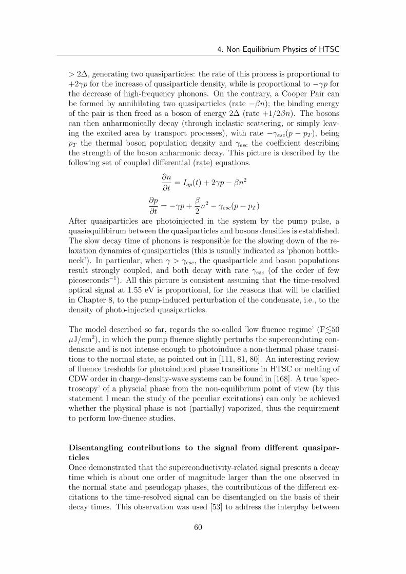
4. Non-Equilibrium Physics of HTSC
> 2∆, generating two quasiparticles: the rate of this process is proportional to+2γp for the increase of quasiparticle density, while is proportional to −γp forthe decrease of high-frequency phonons. On the contrary, a Cooper Pair canbe formed by annihilating two quasiparticles (rate −βn); the binding energyof the pair is then freed as a boson of energy 2∆ (rate +1/2βn). The bosonscan then anharmonically decay (through inelastic scattering, or simply leav-ing the excited area by transport processes), with rate −γesc(p − pT ), beingpT the thermal boson population density and γesc the coefficient describingthe strength of the boson anharmonic decay. This picture is described by thefollowing set of coupled differential (rate) equations.
∂n
∂t= Iqp(t) + 2γp− βn2
∂p
∂t= −γp+
β
2n2 − γesc(p− pT )
After quasiparticles are photoinjected in the system by the pump pulse, aquasiequilibirum between the quasiparticles and bosons densities is established.The slow decay time of phonons is responsible for the slowing down of the re-laxation dynamics of quasiparticles (this is usually indicated as ’phonon bottle-neck’). In particular, when γ > γesc, the quasiparticle and boson populationsresult strongly coupled, and both decay with rate γesc (of the order of fewpicoseconds−1). All this picture is consistent assuming that the time-resolvedoptical signal at 1.55 eV is proportional, for the reasons that will be clarifiedin Chapter 8, to the pump-induced perturbation of the condensate, i.e., to thedensity of photo-injected quasiparticles.
The model described so far, regards the so-called ’low fluence regime’ (F.50µJ/cm2), in which the pump fluence slightly perturbs the superconduting con-densate and is not intense enough to photoinduce a non-thermal phase transi-tions to the normal state, as pointed out in [111, 81, 80]. An interesting reviewof fluence tresholds for photoinduced phase transitions in HTSC or melting ofCDW order in charge-density-wave systems can be found in [168]. A true ’spec-troscopy’ of a physcial phase from the non-equilibrium point of view (by thisstatement I mean the study of the peculiar excitations) can only be achievedwhether the physical phase is not (partially) vaporized, thus the requirementto perform low-fluence studies.
Disentangling contributions to the signal from different quasipar-ticlesOnce demonstrated that the superconductivity-related signal presents a decaytime which is about one order of magnitude larger than the one observed inthe normal state and pseudogap phases, the contributions of the different ex-citations to the time-resolved signal can be disentangled on the basis of theirdecay times. This observation was used [53] to address the interplay between
60
4.2. Pump-Probe experiments and QP dynamics in HTSC
superconducting and pseudogap phases in YBCO crystals. In Fig. 4.5 therelaxation times associated to the different components of a multicomponentexponential fitting to the data are reported. This successful way of disentan-gling the different excitation contributions revealed a temperature independentpseudogap and a temperature-dependent superconducting gap, with BCS-liketemperature dependence. This also implies a possible coexistence of both gapsbelow Tc. The fact that the decay of the superconducting component divergesexactly at Tc can be explained on the basis of the Rothwarf and Taylor model:as the gap ∆ decreases approaching Tc, an increasing number of phonons canbreak Cooper Pairs, and this results in a huge number of quasiparticles. Thus aquasiequilibrium between quasiparticles and phonons establishes, which slowsdown the recombination dynamics, governed only by inelastic processes.
Figure 4.5: Relaxation times resulting from a two component fit of the time-resolved optical signal, on some YBCO samples, differing from the doping level.One component (squares) diverges exactly at T=Tc, while the other (circles)is temperature independent. From [53].
Pump-probe measurements in the THz region
61
4. Non-Equilibrium Physics of HTSC
In the superconducting phase, the signal observed at 1.55 eV is intimately re-lated to the low-energy physics associated to the superconducting condensate.This can be directly demonstrated by pump-probe measurements in which theprobe is a THz field (1 THz= 4.13 meV). In particular, in the THz range, theoptical conductivity is given by the formula [99] (within a two fluid model, forquasiparticle density ρQP and superfluid density ρS):
σ(ω) = ρQP1
1/τ − iω+ ρS
(
πδ(0) +i
ω
)
from which it is clear that the imaginary part σ2(ω) is proportional to thesuperconducting condensate density, at low frequencies (τ is the conventionalDrude scattering time).The THz probe thus directly accesses the superconducting condensate energyregion. Typically, this energy region is 0.1-3 THz, ie, 0.4-12 meV. Examplesof this kind of pump-probe measurements are reported in [12, 99]. The mea-sured THz relaxation dynamics is strikingly similar to that observed in thenear-infrared, as can be argued by looking at Fig. 4.6 (from [99]). Some differ-ence exist anyway with respect to the optical probing: while elastic scatteringwith large momentum transfer dominates transport properties of carriers, thetransient THz kinetics enables a sensitive measure of the inelastic quasiparticlerecombination.
Magnitude of the signal in the different phases of an HTSCThe fact that, in the visible spectral region, the observed transient reflectivitysignal magnitude in the superconducting state (of the order of 10−4 for fluencesof the order of 1 µJ/cm2) is at least one order of magnitude bigger than the oneobserved in the normal state and pseudogap phases, has been known by longtime [164] (see Fig. 4.7). A clear interpratation of this fact has been proposedonly recently [80]. Two scenarios were proposed to explain this experimentalevidence: the first consider the ∆R/R signal as due to an excited state ab-sorption, as it happens in metals and semiconductors. The second, instead,consider the ∆R/R signal as arising from a true (pump-induced) modificationof the band structure of the material, which involves a spectral weight shiftbetween high (in the near-IR) and low (condensate) energy scales (and whichjustifies the increase of the magnitude of the signal). In this scenario, the bandstructure at high energy is modified as a consequence of a partial quench ofthe energy gap, demonstrating an interplay between physics at very differentenergy scales. We ruled out the first scenario [80], as I explain in Chapter 8.
Beyond one-color optical pump-probe measurementsIn concluding this section, I want to remark how single-color measurements,though very powerful in characterizing the peculiar phase of the system and in
62
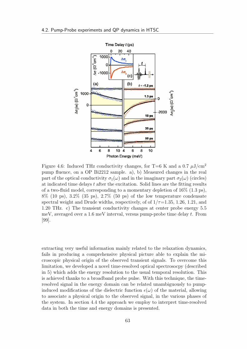
4.2. Pump-Probe experiments and QP dynamics in HTSC
Figure 4.6: Induced THz conductivity changes, for T=6 K and a 0.7 µJ/cm2
pump fluence, on a OP Bi2212 sample. a), b) Measured changes in the realpart of the optical conductivity σ1(ω) and in the imaginary part σ2(ω) (circles)at indicated time delays t after the excitation. Solid lines are the fitting resultsof a two-fluid model, corresponding to a momentary depletion of 16% (1.3 ps),8% (10 ps), 3.2% (35 ps), 2.7% (50 ps) of the low temperature condensatespectral weight and Drude widths, respectively, of of 1/τ=1.35, 1.26, 1.21, and1.20 THz. c) The transient conductivity changes at center probe energy 5.5meV, averaged over a 1.6 meV interval, versus pump-probe time delay t. From[99].
extracting very useful information mainly related to the relaxation dynamics,fails in producing a comprehensive physical picture able to explain the mi-croscopic physical origin of the observed transient signals. To overcome thislimitation, we developed a novel time-resolved optical spectrosocpy (describedin 5) which adds the energy resolution to the usual temporal resolution. Thisis achieved thanks to a broadband probe pulse. With this technique, the time-resolved signal in the energy domain can be related unambiguously to pump-induced modifications of the dielectric function ǫ(ω) of the material, allowingto associate a physical origin to the observed signal, in the various phases ofthe system. In section 4.4 the approach we employ to interpret time-resolveddata in both the time and energy domains is presented.
63
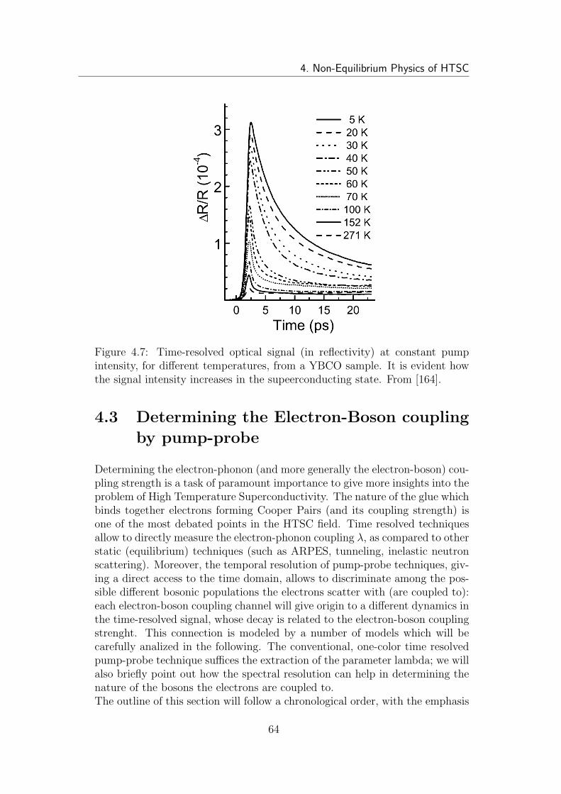
4. Non-Equilibrium Physics of HTSC
Figure 4.7: Time-resolved optical signal (in reflectivity) at constant pumpintensity, for different temperatures, from a YBCO sample. It is evident howthe signal intensity increases in the supeerconducting state. From [164].
4.3 Determining the Electron-Boson coupling
by pump-probe
Determining the electron-phonon (and more generally the electron-boson) cou-pling strength is a task of paramount importance to give more insights into theproblem of High Temperature Superconductivity. The nature of the glue whichbinds together electrons forming Cooper Pairs (and its coupling strength) isone of the most debated points in the HTSC field. Time resolved techniquesallow to directly measure the electron-phonon coupling λ, as compared to otherstatic (equilibrium) techniques (such as ARPES, tunneling, inelastic neutronscattering). Moreover, the temporal resolution of pump-probe techniques, giv-ing a direct access to the time domain, allows to discriminate among the pos-sible different bosonic populations the electrons scatter with (are coupled to):each electron-boson coupling channel will give origin to a different dynamics inthe time-resolved signal, whose decay is related to the electron-boson couplingstrenght. This connection is modeled by a number of models which will becarefully analized in the following. The conventional, one-color time resolvedpump-probe technique suffices the extraction of the parameter lambda; we willalso briefly point out how the spectral resolution can help in determining thenature of the bosons the electrons are coupled to.The outline of this section will follow a chronological order, with the emphasis
64
4.3. Determining the Electron-Boson coupling by pump-probe
on the experimental findings which motivated or supported the various models.In particular, I will start from the Two-Temperature Model (4.1), and then in-troduce the Three-Temperature Model (4.5), illustrating the reasons leading tothe formlation of this model. I will also formulate a novel, generalized versionof the three temperature model, in which a ’parallel’ coupling of electrons withall bosonic populations is taken into account (4.8). This model can be natu-rally extended to include more temperatures, one for each bosonic populationthe electrons scatter with. On this line, I will present the system of coupleddifferential equations for a four temperature model. With this model, formu-lated to explain the experimental evidences presented in 6, all the possiblescattering mechanisms which contributes to the total electron-boson pairing,which manifests in the glue function Π(Ω), are taken into account.
4.3.1 The Two-Temperature Model
In this section, the Two-Temperature Model (2TM) is described.The so-called ’Two-Temperature Model’ is the result of the theoretical workdone by Anisimov [10] and Allen [7]. The model interprets and describes theelectronic non-equilibrium dynamics excited in a material by an ultrashort(∼100 fs) laser light pulse. This model applies to metals and conventional,metallic superconductors. The formulation of this model was stimulated bythe development of new laser sources, producing ultrashort pulses in the psdomain. The first systematic experimental studies were those of Brorson [25],who measured λ in several metals.We can say that the two temperature model describes the physics of a pump-probe experiment carried on a solid state material, in which the electron-phonon scattering is directly observed in the time domain.The physical picture on which the model was developed is the following. Theenergy deposited in the system by the laser pulse is absorbed by electrons,which are instantaneously excited above the Fermi level. After a few fs,electron-electron scattering processes, on the 1-10 fs timescale [11], drive thethermalization of the electronic population at an elevated temperature Te > T0,T0 being the base temperature. On this timescale, the electrons are practicallydisentangled from the lattice: the electrons thus reach the maximum tempera-ture Te(0) determined mainly by their specific heat. On a longer timescale, theelectrons start to lose energy through electron-phonon scattering, and reacha common temperature with phonons. Finally, a much slower relaxation pro-cess - dominated by heat diffusion - makes the system return to the ambienttemperature T0. It is important to point out that the rate of return to lo-cal equilibrium is governed entirely by electron-phonon processes. The modelpresented assumes that diffusion driven by spatial inhomogeneities is negligi-ble; acceleration due to both external and internal fields is negligible, and noother collision processes are important. The most important requirement isthat electron-electron and phonon-phonon (anharmonic) processes are activein keeping the electronic and phononic distributions equal to the local equi-
65
4. Non-Equilibrium Physics of HTSC
librium distributions (respectively FD and BE) at the separated temperaturesTe(t) and Tl(t). The metal is looked as a two temperature system at everytime t.The phenomenologic system of coupled differential equations describing theevolution of the electronic and the lattice temperatures, as proposed by Anisi-mov in 1974 to describe the energy balance for a metal absorbing a laser pulse,is:
∂Te
∂t= − G
Ce
(Te − Tl) +p
Ce
(4.1a)
∂Tl
∂t=
G
Cl
(Te − Tl) (4.1b)
Where Te, Tl are the electronic and lattice (phonon) temperatures, respec-tively. G = γe−phCe is a coupling constant describing the coupling between theelectron and the phonon systems. γe−ph is a different way of expressing thecoupling constant, often found in the literaure [7]. Ce = γeTe is the electronicspecific heat, being γe the coefficient of the linear electronic specific heat. Cl
is the lattice specific heat. p is the absorbed power, with the same Gaussianprofile of the laser pulse. Both the specific heats and the laser power are ex-pressed per unit of volume.The solution of this system of equations indicates that the electronic tempera-ture evolution follows an exponential decay with time-constant τ = (γe−ph)
−1.It is worth to point out that this model was developed in order to describethe electron emission from metal surfaces exposed to picosecond laser pulses.It was found that for laser intensities beyond a critical value, the emissioncurrent is entirely due to thermoionic emission (while below threshold a com-petition between photoelectric emission and thermoionic emission exists). Thefirst attempt to measure the electron-lattice relaxation kinetics was done bymeasuring the thermoionic emission current, proportional to the electronictemperature.The relation between the experimentally measured τ and the key-quantity λ,expressing the electron-phonon coupling in the superconductivity theory, hasbeen first derived by Allen [7], though in a limit I will discuss in the following.The main result is that λ can be directly inferred from τ , once the electronictemperature Te and the mean phonon energy 〈~2ω2〉 are known. Allen’s for-mula is:
γe−ph =3λ〈~2ω2〉~πk2
BTe
(4.2)
thus:
G = γe−phγeTe =3γe~πk2
B
λ〈~2ω2〉
Te(0) can be easily evaluated starting from the pump laser energy delivered tothe electrons, and the electronic specific heat. This value, together with thevalue of Te(∞)=Tl(∞) (which can be estimated from the pump laser energy
66
4.3. Determining the Electron-Boson coupling by pump-probe
and the lattice specific heat), constitute the initial conditions to correctly solvethe differential system of equations (while Tl(0) = T0, being T0 the base systemtemperature). The mean phonon energy 〈~2ω2〉 is more difficult to evaluate;it can be taken from the literature (the phonon spectrum can be measuredby scattering techniques), or it can be approximated with ~
2ωD2/2 [24]. Since
Te(0) can be calculated, measuring τ allows to know the product λ〈~2ω2〉 with-out free parameters. For completeness, the experimentally extracted values ofλ range from 0.1 to 0.15 for non-superconducting metals (Au, Cu), to 0.25-0.4for very low-Tc (.1 K) superconductors (W, Ir, Ti, Zn), to 0.8-1 for the mostknown metallic superconductors (In, Sn, Hg, Pb, Nb), which are in the strong-coupling limit.Expression 4.2 predicts a direct proportionality between the decay time τ andthe electronic temperature Te. To understand in which limits this formula isapplicable, it is worth to follow a few steps, illustrating the approximationsused and the derivation of the same expression.The decay rate of the electron thermal energy (transferred to the phonon sys-tem) is given by:
∂Ee
∂t= 2πNcN(EF )
∫ ∞
0
dΩα2F (Ω)(~Ω)2 [N(Ω, Tl)−N(Ω, Te)] (4.3)
where Nc is the number of cells in the sample, N(EF ) is the density of states ofboth spins per unit cell, and N(Ω, Tj) are the BE distribution functions (j=e,l).The electronic energy for the system can be written as: Ee =
∑
k ǫkFk ≈E0 + 1/2γeT
2e (where Fk is the FD distribution, and E0 the system point-zero
energy, for the system at T = 0), while the electronic specific heat writes:γe=π2NcN(EF )k
2B/3.
Without any assumption regarding the actual spectrum of the electron-phononcoupling α2F (Ω), and remembering that λ 〈ω2〉 = 2
∫∞
0α2F (Ω)ΩdΩ, equation
4.3 can be rewritten as:
∂Ee
∂t= π~NcN(EF )λ
⟨
ω2⟩
kB(Tl − Te) + ... (4.4)
if a Taylor expansion of N(Ω, Tj) in terms of ~Ω/kBTj is carried out, in thehigh temperature limit, that is, when both Te and Tl are much higher thanthe phonon energy ~Ω.Finally, expression 4.4 can be recasted in the usual form ∂Te/∂t = γe−ph(Tl−Te)by using the definitions of EE and γe.Allen Formula 4.2 is thus strictly valid only when the system is considerablyheated by the pump pulse energy.
Relation between the optical signal and the temperature increments∆Te, ∆Tl
In the context of a pump-probe experiment, the pump-induced change of theelectronic temperature Te modifies the electronic distribution of the material,
67
4. Non-Equilibrium Physics of HTSC
being the electronic population described by a Fermi-Dirac statistic at an el-evated temperature Te. This effect can be monitored by a subsequent probepulse, which reflection or transmission is influenced by the change in the elec-tronic population of the material. More considerations about this point aredone at the end of this section.It must be emphasized that, for the optical pump-probe technique to be em-ployed to the study of the electron-phonon coupling, the induced changes inTj (j=e,l) must have an effect on the sample optical properties (reflectivity ortransmittivity), at the probe wavelength. In the more general form, the in-duced change in reflectivity will be sensitive to both variations in the electronictemperature (∆Te) and in the lattice one (∆Tl): ∆R/R = c1 ·∆Te + c2 ·∆Tl.The ratio c1/c2 is usually a free fitting parameter.Changes due to ∆Tl can come from band shifting arising from thermal strain.These lattice-temperature-induced reflectivity changes will decay on very longtimescales, determined by the rate at which the heat can diffuse away fromthe optically excited area. In this model Te and Tl remain at an elevated tem-perature with respect to T0, since the heat diffusion effect is not taken intoaccount. This is not a limitation, being the timescale of this effect of the orderof the ns.Changes induced by ∆Te instead are due to optical transition from/to stateswhich population is altered by the laser excitation; in particular, any transitioninvolving states near the Fermi level will be sensitive to Te. The idea is simple:the increase of the electronic population makes the tails of the Fermi distribu-tion smearing, opening states below the Fermi level for transitions. These newstates can then absorb probe photons, resulting in an increase of absorption.Alternatively, the promoted electrons of the Fermi distribution can be excitedto free states above the Fermi level, resulting in an absorption decrease. Theactual sign of the ∆R/R thus depends upon the material band structure.Overall, the relative induced change in reflectivity turns out to be very small,of the order of 10−4 to 10−6.
Limits of the Two-Temperature ModelHere I will state briefly the main limits of the 2TM, which call for an exten-sion of the model. The main criticism to this model stands in the possibilityto define the electronic temperature Te. Though the optical scattering rateτe−e is of the order 1-10 fs [11], indicating a very fast electron thermalization,recent photoemission experiments [145] found a small deviation of the actualnon-equilibrium electronic distribution with respect to a Fermi-Dirac statistics.The non-thermalized high-energy tail evidenced in [145], to whom the authorsdidn’t give much weight, is instead predicted (as shown in [75]) by exact cal-culations [96] taking into account the exact analytical solution of the integralBoltzmann equation, without the questionable assumption that electrons arein a quasiequilibrium with a time-dependent temperature. The electron-latticeralaxation rate within this formalism is: (τe−ph)
−1 = 3~λ 〈ω2〉 /2πkBTl. Apart
68
4.3. Determining the Electron-Boson coupling by pump-probe
the factor of ’2’ with respect to the 2TM result, more important is the de-pendence on Tl rather than Te, which justifies the experimental evidence thatthe relaxation rate is fluence-independent. A term of difficult evaluation is〈ω2〉, which is in general taken from the literature. The model by Kabanovet al. [96], which is applicable also when the electron-electron scattering timeis bigger than the electron-phonon scattering time (i.e., when τe−e>τe−ph), isthe natural model to be employed to interpret the findings described in [144],in which the apex oxygen vibration in YBCO turns out to be strongly excitedwithin 150 fs, demonstrating that the lattice absorbs a major portion of thepump energy before the quasiparticles are thermalized. The evidence of anultrafast electron-phonon coupling with peculiar phononic modes, evidencedin [144], and the observation of a double exponentially-decaying dynamicsin optical measurements on HTSC, are a strong evidence for an anisotropicelectron-phonon coupling, which cannot be accounted for by the 2TM. Thisobservation clearly invokes a further coupling term, which is accounted for bythe Three-Temperature Model.
4.3.2 The Three-Temperature Model
The Three-Temperature Model (3TM) was initially developed [145] as an ex-tended version of the two temperature model, to interpret recent new resultsobtained with the time-resolved ARPES technique. In particular, this modelwell reproduces the time-resolved dynamics observed in systems with a stronganisotropy of the electron-phonon interaction, due to phonon branches withdifferent coupling strength, which results in different timescales in the relax-ation dynamics. This is the case of strongly correlated materials, such as thecuprates.The experimental findings, on an optimally doped Bi2212 single crystal (atT=30K), are the following. A time-resolved ARPES experiment is concep-tually simple: the sample excitation is performed with 1.5 eV laser pulses(pump), while the photoelectrons are emitted thanks to a 6 eV probe beamwhich is delayed with respect to the former. Photoelectrons are collected andanalyzed with a time-of-flight (TOF) spectrometer. Time-resolved ARPES’directly’ probes the electronic temperature Te(t), which is inferred from thephotoelectron spectra (collected at the Fermi wavevector) at various pump-probe delays t. A fast thermalization for the electronic population is observed,since the electronic distribution converges to a Fermi Dirac distribution withinthe pump pulse duration (∼50 fs). This is due to a large electron-electroninteraction. The novelty of the data stands in the fact that the electronictemperature Te relaxes with two different timescales: a fast one (which relaxeswith an exponential decay with τα ≈110 fs) and a slow one (which decays withτβ ≈2 ps).The physical interpretation the authors gave was the following. After thefast electronic thermalization, the electronic population at the temperatureTe starts to relax transferring energy to a subset of strongly coupled (also
69
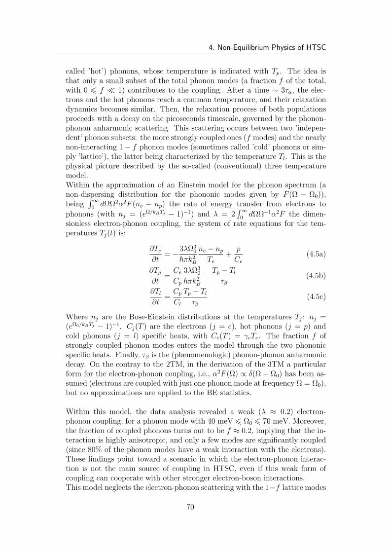
4. Non-Equilibrium Physics of HTSC
called ’hot’) phonons, whose temperature is indicated with Tp. The idea isthat only a small subset of the total phonon modes (a fraction f of the total,with 0 6 f ≪ 1) contributes to the coupling. After a time ∼ 3τα, the elec-trons and the hot phonons reach a common temperature, and their relaxationdynamics becomes similar. Then, the relaxation process of both populationsproceeds with a decay on the picoseconds timescale, governed by the phonon-phonon anharmonic scattering. This scattering occurs between two ’indepen-dent’ phonon subsets: the more strongly coupled ones (f modes) and the nearlynon-interacting 1− f phonon modes (sometimes called ’cold’ phonons or sim-ply ’lattice’), the latter being characterized by the temperature Tl. This is thephysical picture described by the so-called (conventional) three temperaturemodel.Within the approximation of an Einstein model for the phonon spectrum (anon-dispersing distribution for the phononic modes given by F (Ω − Ω0)),being
∫∞
0dΩΩ2α2F (ne − np) the rate of energy transfer from electrons to
phonons (with nj = (eΩ/kBTj − 1)−1) and λ = 2∫∞
0dΩΩ−1α2F the dimen-
sionless electron-phonon coupling, the system of rate equations for the tem-peratures Tj(t) is:
∂Te
∂t= −3λΩ3
0
~πk2B
ne − np
Te
+p
Ce
(4.5a)
∂Tp
∂t=
Ce
Cp
3λΩ30
~πk2B
− Tp − Tl
τβ(4.5b)
∂Tl
∂t=
Cp
Cl
Tp − Tl
τβ(4.5c)
Where nj are the Bose-Einstein distributions at the temperatures Tj: nj =(eΩ0/kBTj − 1)−1. Cj(T ) are the electrons (j = e), hot phonons (j = p) andcold phonons (j = l) specific heats, with Ce(T ) = γeTe. The fraction f ofstrongly coupled phonon modes enters the model through the two phononicspecific heats. Finally, τβ is the (phenomenologic) phonon-phonon anharmonicdecay. On the contray to the 2TM, in the derivation of the 3TM a particularform for the electron-phonon coupling, i.e., α2F (Ω) ∝ δ(Ω− Ω0) has been as-sumed (electrons are coupled with just one phonon mode at frequency Ω = Ω0),but no approximations are applied to the BE statistics.
Within this model, the data analysis revealed a weak (λ ≈ 0.2) electron-phonon coupling, for a phonon mode with 40 meV 6 Ω0 6 70 meV. Moreover,the fraction of coupled phonons turns out to be f ≈ 0.2, implying that the in-teraction is highly anisotropic, and only a few modes are significantly coupled(since 80% of the phonon modes have a weak interaction with the electrons).These findings point toward a scenario in which the electron-phonon interac-tion is not the main source of coupling in HTSC, even if this weak form ofcoupling can cooperate with other stronger electron-boson interactions.This model neglects the electron-phonon scattering with the 1−f lattice modes
70
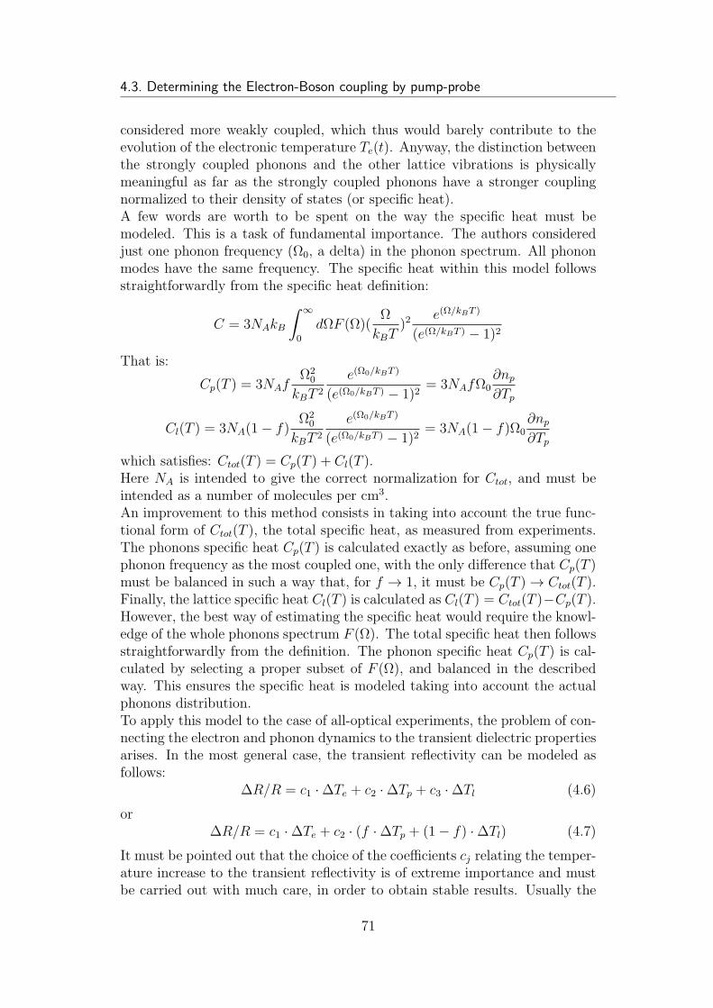
4.3. Determining the Electron-Boson coupling by pump-probe
considered more weakly coupled, which thus would barely contribute to theevolution of the electronic temperature Te(t). Anyway, the distinction betweenthe strongly coupled phonons and the other lattice vibrations is physicallymeaningful as far as the strongly coupled phonons have a stronger couplingnormalized to their density of states (or specific heat).A few words are worth to be spent on the way the specific heat must bemodeled. This is a task of fundamental importance. The authors consideredjust one phonon frequency (Ω0, a delta) in the phonon spectrum. All phononmodes have the same frequency. The specific heat within this model followsstraightforwardly from the specific heat definition:
C = 3NAkB
∫ ∞
0
dΩF (Ω)(Ω
kBT)2
e(Ω/kBT )
(e(Ω/kBT ) − 1)2
That is:
Cp(T ) = 3NAfΩ2
0
kBT 2
e(Ω0/kBT )
(e(Ω0/kBT ) − 1)2= 3NAfΩ0
∂np
∂Tp
Cl(T ) = 3NA(1− f)Ω2
0
kBT 2
e(Ω0/kBT )
(e(Ω0/kBT ) − 1)2= 3NA(1− f)Ω0
∂np
∂Tp
which satisfies: Ctot(T ) = Cp(T ) + Cl(T ).Here NA is intended to give the correct normalization for Ctot, and must beintended as a number of molecules per cm3.An improvement to this method consists in taking into account the true func-tional form of Ctot(T ), the total specific heat, as measured from experiments.The phonons specific heat Cp(T ) is calculated exactly as before, assuming onephonon frequency as the most coupled one, with the only difference that Cp(T )must be balanced in such a way that, for f → 1, it must be Cp(T ) → Ctot(T ).Finally, the lattice specific heat Cl(T ) is calculated as Cl(T ) = Ctot(T )−Cp(T ).However, the best way of estimating the specific heat would require the knowl-edge of the whole phonons spectrum F (Ω). The total specific heat then followsstraightforwardly from the definition. The phonon specific heat Cp(T ) is cal-culated by selecting a proper subset of F (Ω), and balanced in the describedway. This ensures the specific heat is modeled taking into account the actualphonons distribution.To apply this model to the case of all-optical experiments, the problem of con-necting the electron and phonon dynamics to the transient dielectric propertiesarises. In the most general case, the transient reflectivity can be modeled asfollows:
∆R/R = c1 ·∆Te + c2 ·∆Tp + c3 ·∆Tl (4.6)
or∆R/R = c1 ·∆Te + c2 · (f ·∆Tp + (1− f) ·∆Tl) (4.7)
It must be pointed out that the choice of the coefficients cj relating the temper-ature increase to the transient reflectivity is of extreme importance and mustbe carried out with much care, in order to obtain stable results. Usually the
71
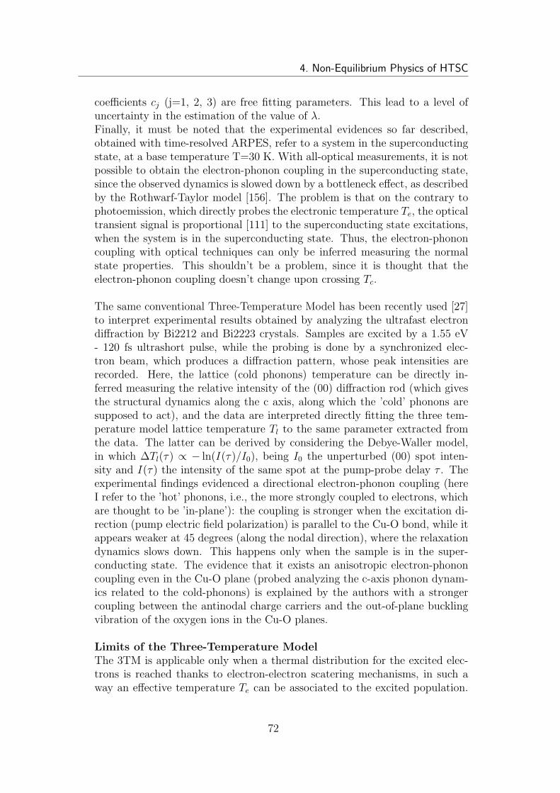
4. Non-Equilibrium Physics of HTSC
coefficients cj (j=1, 2, 3) are free fitting parameters. This lead to a level ofuncertainty in the estimation of the value of λ.Finally, it must be noted that the experimental evidences so far described,obtained with time-resolved ARPES, refer to a system in the superconductingstate, at a base temperature T=30 K. With all-optical measurements, it is notpossible to obtain the electron-phonon coupling in the superconducting state,since the observed dynamics is slowed down by a bottleneck effect, as describedby the Rothwarf-Taylor model [156]. The problem is that on the contrary tophotoemission, which directly probes the electronic temperature Te, the opticaltransient signal is proportional [111] to the superconducting state excitations,when the system is in the superconducting state. Thus, the electron-phononcoupling with optical techniques can only be inferred measuring the normalstate properties. This shouldn’t be a problem, since it is thought that theelectron-phonon coupling doesn’t change upon crossing Tc.
The same conventional Three-Temperature Model has been recently used [27]to interpret experimental results obtained by analyzing the ultrafast electrondiffraction by Bi2212 and Bi2223 crystals. Samples are excited by a 1.55 eV- 120 fs ultrashort pulse, while the probing is done by a synchronized elec-tron beam, which produces a diffraction pattern, whose peak intensities arerecorded. Here, the lattice (cold phonons) temperature can be directly in-ferred measuring the relative intensity of the (00) diffraction rod (which givesthe structural dynamics along the c axis, along which the ’cold’ phonons aresupposed to act), and the data are interpreted directly fitting the three tem-perature model lattice temperature Tl to the same parameter extracted fromthe data. The latter can be derived by considering the Debye-Waller model,in which ∆Tl(τ) ∝ − ln(I(τ)/I0), being I0 the unperturbed (00) spot inten-sity and I(τ) the intensity of the same spot at the pump-probe delay τ . Theexperimental findings evidenced a directional electron-phonon coupling (hereI refer to the ’hot’ phonons, i.e., the more strongly coupled to electrons, whichare thought to be ’in-plane’): the coupling is stronger when the excitation di-rection (pump electric field polarization) is parallel to the Cu-O bond, while itappears weaker at 45 degrees (along the nodal direction), where the relaxationdynamics slows down. This happens only when the sample is in the super-conducting state. The evidence that it exists an anisotropic electron-phononcoupling even in the Cu-O plane (probed analyzing the c-axis phonon dynam-ics related to the cold-phonons) is explained by the authors with a strongercoupling between the antinodal charge carriers and the out-of-plane bucklingvibration of the oxygen ions in the Cu-O planes.
Limits of the Three-Temperature ModelThe 3TM is applicable only when a thermal distribution for the excited elec-trons is reached thanks to electron-electron scatering mechanisms, in such away an effective temperature Te can be associated to the excited population.
72
4.3. Determining the Electron-Boson coupling by pump-probe
Thus it is not applicable when a gap in the density of states is opened. The3TM is thus stictly applicable to HTSC only at room temperature and on theOP and OD regions of the phase diagram. It is well-known that in cupratesuperconductors [77], in the superconducting state, the probed excitations arequasiparticles which occupy a precise region of k-space, and namely the antin-odal one, where the gap has its maximum. Thus, the probed excitations have astrongly non-thermal distribution, which impedes the application of the 3TMto reproduce the measured dynamics. The fact that a non-thermal distributionof excitations is obtained in the presence of a gap is explained by the block-ing of electron-electron scattering away from the node, because of the limitedphase space in the antinodal region. Recently, this speculation has been ob-served experimentally by time-resolved photoemission experiments, analyzingthe electronic thermalization in various k-directions of the Brillouin zone of aBi2212 sample [41].In the conventional 3TM, electrons are directly coupled only with the so-calledstrongly-coupled phonons. To take into account the direct coupling of electronswith different kinds of bosonic excitations, we propose a generalized version ofthe 3TM, accounting for the energy exchange among the different degrees offreedom of a system in a phenomenological way.
4.3.3 A generalized Three-Temperature Model
In order to overcome some of the limitations of the conventional three tem-perature model, and to provide a model which is able to fully reproduce therelaxation dynamics of a system whose electron-boson coupling is describedby a general bosonic glue Π(Ω) made of different contributions, we developeda new model in which we assign a temperature Tj (j=p for storngly coupledphonons, j=l for weakly coupled phonons or lattice) to each different bosonicpopulation the electrons scatter with, and whose coupling λj (here again j=p,l)with the electrons derives from a particular subset Πj(Ω) of the total bosonicglue Π(Ω):
λj = 2
∫ ∞
0
dΩΠj(Ω)
Ω
where: Π(Ω) =∑N
j=1Πj(Ω); obviously λ =∑N
j=1 λj.The various Πj(Ω) linearly contribute to the total bosonic glue Π(Ω), whichthus accounts for all the possible degrees of freedom the electrons can exchangeenergy with. N defines the number of temperatures (and degrees of freedom)considered in the model.If we consider only phonons (both strongly and weakly coupled) as possiblemediator bosons, we obtain a three temperature model in which the phonon-phonon anharmonic coupling term is replaced by a direct electron-weakly-coupled-phonon interaction term, which carries a coupling strength λl (absentin the conventional three temperature model). The model we propose is thefollowing (here the anharmonic term has been completely neglected, but it can
73
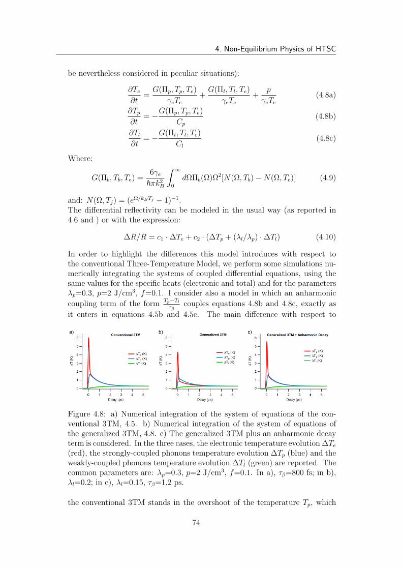
4. Non-Equilibrium Physics of HTSC
be nevertheless considered in peculiar situations):
∂Te
∂t=
G(Πp, Tp, Te)
γeTe
+G(Πl, Tl, Te)
γeTe
+p
γeTe
(4.8a)
∂Tp
∂t= −G(Πp, Tp, Te)
Cp
(4.8b)
∂Tl
∂t= −G(Πl, Tl, Te)
Cl
(4.8c)
Where:
G(Πb, Tb, Te) =6γe~πk2
B
∫ ∞
0
dΩΠb(Ω)Ω2[N(Ω, Tb)−N(Ω, Te)] (4.9)
and: N(Ω, Tj) = (eΩ/kBTj − 1)−1.The differential reflectivity can be modeled in the usual way (as reported in4.6 and ) or with the expression:
∆R/R = c1 ·∆Te + c2 · (∆Tp + (λl/λp) ·∆Tl) (4.10)
In order to highlight the differences this model introduces with respect tothe conventional Three-Temperature Model, we perform some simulations nu-merically integrating the systems of coupled differential equations, using thesame values for the specific heats (electronic and total) and for the parametersλp=0.3, p=2 J/cm3, f=0.1. I consider also a model in which an anharmonic
coupling term of the form Tp−Tl
τβcouples equations 4.8b and 4.8c, exactly as
it enters in equations 4.5b and 4.5c. The main difference with respect to
Figure 4.8: a) Numerical integration of the system of equations of the con-ventional 3TM, 4.5. b) Numerical integration of the system of equations ofthe generalized 3TM, 4.8. c) The generalized 3TM plus an anharmonic decayterm is considered. In the three cases, the electronic temperature evolution ∆Te
(red), the strongly-coupled phonons temperature evolution ∆Tp (blue) and theweakly-coupled phonons temperature evolution ∆Tl (green) are reported. Thecommon parameters are: λp=0.3, p=2 J/cm3, f=0.1. In a), τβ=800 fs; in b),λl=0.2; in c), λl=0.15, τβ=1.2 ps.
the conventional 3TM stands in the overshoot of the temperature Tp, which
74
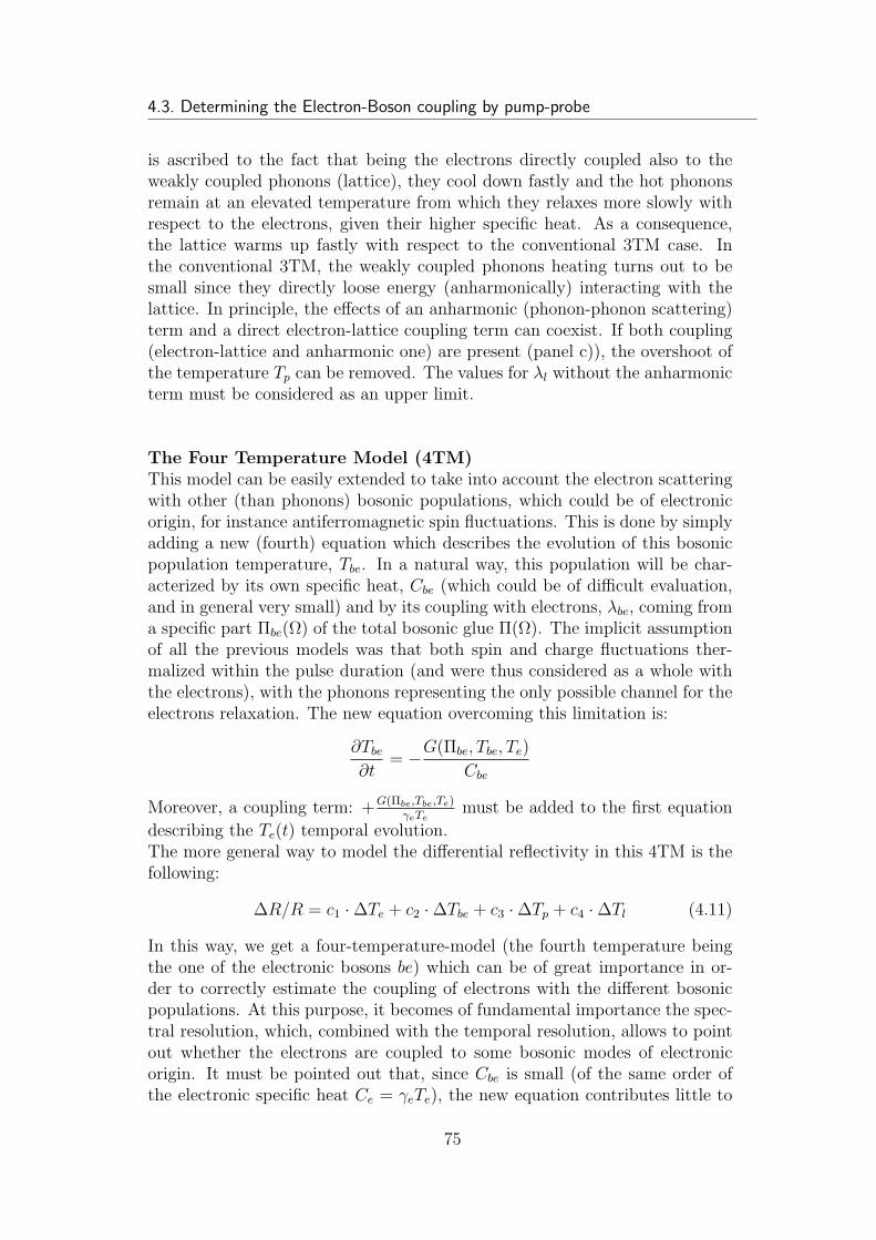
4.3. Determining the Electron-Boson coupling by pump-probe
is ascribed to the fact that being the electrons directly coupled also to theweakly coupled phonons (lattice), they cool down fastly and the hot phononsremain at an elevated temperature from which they relaxes more slowly withrespect to the electrons, given their higher specific heat. As a consequence,the lattice warms up fastly with respect to the conventional 3TM case. Inthe conventional 3TM, the weakly coupled phonons heating turns out to besmall since they directly loose energy (anharmonically) interacting with thelattice. In principle, the effects of an anharmonic (phonon-phonon scattering)term and a direct electron-lattice coupling term can coexist. If both coupling(electron-lattice and anharmonic one) are present (panel c)), the overshoot ofthe temperature Tp can be removed. The values for λl without the anharmonicterm must be considered as an upper limit.
The Four Temperature Model (4TM)This model can be easily extended to take into account the electron scatteringwith other (than phonons) bosonic populations, which could be of electronicorigin, for instance antiferromagnetic spin fluctuations. This is done by simplyadding a new (fourth) equation which describes the evolution of this bosonicpopulation temperature, Tbe. In a natural way, this population will be char-acterized by its own specific heat, Cbe (which could be of difficult evaluation,and in general very small) and by its coupling with electrons, λbe, coming froma specific part Πbe(Ω) of the total bosonic glue Π(Ω). The implicit assumptionof all the previous models was that both spin and charge fluctuations ther-malized within the pulse duration (and were thus considered as a whole withthe electrons), with the phonons representing the only possible channel for theelectrons relaxation. The new equation overcoming this limitation is:
∂Tbe
∂t= −G(Πbe, Tbe, Te)
Cbe
Moreover, a coupling term: +G(Πbe,Tbe,Te)γeTe
must be added to the first equation
describing the Te(t) temporal evolution.The more general way to model the differential reflectivity in this 4TM is thefollowing:
∆R/R = c1 ·∆Te + c2 ·∆Tbe + c3 ·∆Tp + c4 ·∆Tl (4.11)
In this way, we get a four-temperature-model (the fourth temperature beingthe one of the electronic bosons be) which can be of great importance in or-der to correctly estimate the coupling of electrons with the different bosonicpopulations. At this purpose, it becomes of fundamental importance the spec-tral resolution, which, combined with the temporal resolution, allows to pointout whether the electrons are coupled to some bosonic modes of electronicorigin. It must be pointed out that, since Cbe is small (of the same order ofthe electronic specific heat Ce = γeTe), the new equation contributes little to
75
4. Non-Equilibrium Physics of HTSC
the electronic temperature evolution, and Tbe ≈ Te (this happens also in thevery first part of the relaxation dynamics, during the pulse duration). Thepoint is that the population j = be carries a finite value of λbe. The spectralresolution can help in pointing out what is the true temperature evolution ofthe system, with the following argument: according to the Extended Drudemodel, the electronic temperature can be disentangled from the bosonic one(see sections 3.5.2, 3.5.3), and the fact that Te ≈ Tbe or Te > Tbe gives differ-ent spectral responses (see the simulations reported in 4.4 and the analysis inChapter 6). If the spectral response at early pump-probe delays is in agree-ment with the one simulated in the case Te ≈ Tbe, it means that a bosonicpopulation with small specific heat (and thus of electronic origin) is coupledwith the electrons. Indeed, if electrons were coupled only with phonons, itcouldn’t be Te ≈ Tbe at early delays, for considerations regarding the phononsspecific heat Cp, which makes the phonons warming on longer timescales. Theformer situation revealed the actual one, as pointed out in Chapter 6. Timeresolved spectroscopy thus revealed a powerful technique in order to assign thecorrect value of λ to the various bosonic populations. The relations Tc = Tc(λ)presented in 2.4 finally allowed to clarify which bosonic population is responsi-ble for the actual material Tc. Moreover, the spectral resolution allows both toevaluate the subsets Πj(Ω) of Π(Ω) related to the various bosonic populations(being Π(Ω) determined from static measurements) and to fix the coefficientscj in expression 4.11, thus limiting the number of free parameters of the fit.The results revealed a strong (λ ≈ 1) electron-boson coupling, with bosonswhich are other than phonons, and must thus be of electronic origin. Con-cluding, we can say that in HTSC a strong electron-boson coupling is hiddenfrom the point of view of the electron dynamics, but its actual presence is re-vealed by the spectral resolution. Non-equilibrium spectroscopy thus revealeda very powerful and unique technique in order to shed light on the problem ofelectron-boson coupling in strongly correlated materials.
4.3.4 Modeling the absorbed power density
In this section some considerations about the power density p [J/(cm3·s)],deposited by the laser pulse in the system, are done.The following equalities hold:
p(t) = p02√ln 2√π
e−4 ln 2 t2
τ2 =P0
V
2√ln 2√π
e−4 ln 2 t2
τ2 =E
V · τ2√ln 2√π
e−4 ln 2 t2
τ2
Where p0 is the pulse mean power density, P0 is the pulse mean power, E theenergy per pulse, V the volume in which the energy is deposited, and τ thepulse temporal FWHM , determined for example by auto- or cross-correlationmeasurements.Usually, the volume V is calculated as follows: V = A ·d = π(FWHM/2)2α−1,that is, the excited volume is a cylinder which top area is that of a disk of diam-eter FWHM (determined experimentally), and which height is the penetration
76
4.3. Determining the Electron-Boson coupling by pump-probe
depth d, the inverse of the (wavelength dependent) absorption coefficient α.To improve the model and obtain more reliable results, two steps are required.The first is to take into account the actual shape of the pump pulse (Gaussian)and the finite size of the probe pulse, which is Gaussian too. The second isto consider the role of the finite penetration depth of the pump pulse. Thisis done numerically, calculating ∆R/R(ω) through a transfer matrix method,when a graded index with exponential profile proportional to exp(−z/d) (be-ing d the pump pulse penetration depth) is assumed.
Gaussian Profile for pump and probe beamsAs far as the probe lateral size is kept smaller than the pump one (as alwayshappens in pump-probe experiments), the common procedure for calculatingthe effective power density would be correct if the power distribution wereuniform in the beams section (disk). This is not the case, since the lateralpulse profile is Gaussian. Thus, the actual Gaussian power distribution (givenby the pump pulse) must be taken into account, together with the Gaussianprobe pulse profile. The idea is to calculate which is the effective power densityto be considered in the simulations, with respect to the one calculated in thehomogeneous case, in order to be more quantitative.A Gaussian power distribution for the pump pulse has been taken into account,which is normalized in such a way the total absorbed mean power P is the sameof the homogeneous case (defined by the relation P = p·(πFWHM2/4), wherenow I omitted the temporal dependence):
p ln 2e−4 ln 2r2/FWHM2pu
(indeed:∫ 2π
0
∫∞
0rdrp ln 2e−4 ln 2r2/F 2
pu = P )In the same way, a Gaussian distribution for the probe has been taken intoaccount, which is normalized to ’one’:
4 ln 2
πF 2pr
e−4 ln 2r2/F 2pr
(indeed:∫ 2π
0
∫∞
0rdr 4 ln 2
πF 2pre−4 ln 2r2/F 2
pr = 1)
The effective power density in the non-homogeneous case thus results:
peff = p ln 2
∫ 2π
0
∫ ∞
0
rdre−4 ln 2r2/F 2pr4 ln 2
πF 2pu
e−4 ln 2r2/F 2pr = p ln 2
F 2pu
F 2pu + F 2
pr
If one considers the power distribution ratio with respect to that of the homo-geneous case, it results:
peff/p = ln 2F 2pu
F 2pu + F 2
pr
which depends on the relative spot sizes of the pump and the probe beams.This relation indicates that the measured signal (obviously related to the Gaus-sian case) refers to an effective power which is always smaller than the one
77
4. Non-Equilibrium Physics of HTSC
calculated in the homogeneous case. This means that in the simulations theactual power density must be reduced by a factor which is at least ln 2 ∼0.69,in the case of a delta-like probe. If the probe spot size is one-third the pumpone, the factor becomes: 0.9 · ln 2 ∼0.62; if the probe spot size is half the pumpone, the factor results 0.8 · ln 2 ∼0.55. As far as the probe spot size becomescloser to the pump one, the measured ∆R/R reduces, and the correction withrespect to the homogeneous case is important and important.
Role of the pump-beam finite penetration depthTo get quantitative results in models requiring a precise knowledge of the abso-lute magnitude of a time-resolved signal, the problem of the finite penetrationdepth must be faced. This is the case of the two, three and four temepraturemodels presented so far.The correction which takes into account this effect must be evaluated in a nu-merical way. We employed the transfer matrix method. This method is widelyused in optics to analyze the propagation of electromagnetic waves (here theprobe ones) through a layered medium (in our case, the medium is made op-tically inhomogeneous by the effect of the laser excitation with a pump pulsewhose penetration depth exponentially decays inside the material, and whichinduces a modulation in the material refraction index). The reflection andtransmission of light from an interface between two media is described by theFresnel equations, and is governed by the refraction index (which will thusbe the natural quantity to consider). When multiple interfaces are present,multiple reflections occur. Depending on the geometry of the reflection (whichdetermines the light path length), the reflections can interfere constructively ordestructively (for simplicity we will consider the case of normal incidence). Theoverall reflection and transmission of a layered structure is the result of a hugenumber of reflections, which is in general difficult to calculate. The trans-fer matrix method was developed to this purpose. According to Maxwell’sequations, there are simple continuity conditions for the electric fields acrossboundaries from one layer to the next. If the field is known at the beginningof one layer, the resulting one at the end of the layer can be obtained froma simple matrix operation. The effect of a stack of layers can be representedas the product of the individual layer matrices. The final step of the methodinvolves converting the fields back to reflection and transmission coefficients.We assume the exponentially decaying pump power profile modulates the (com-plex) refraction index in a linear way: the pump-induced modification of therefraction index will thus decay exponentially too in the direction perpen-dicular to the sample surface. The fact that
∫∞
0dze−z/d = d ensures that
the pump-induced modification of the refraction index at the sample surfaceequals the one calculated in the homogeneous case (in which the excited areais a cylinder of height d = α−1). This is helpful since one can consider, asa starting point for the simulation, the transient refraction index values ob-tained in the homogeneous case. The pump-induced modification of n then
78
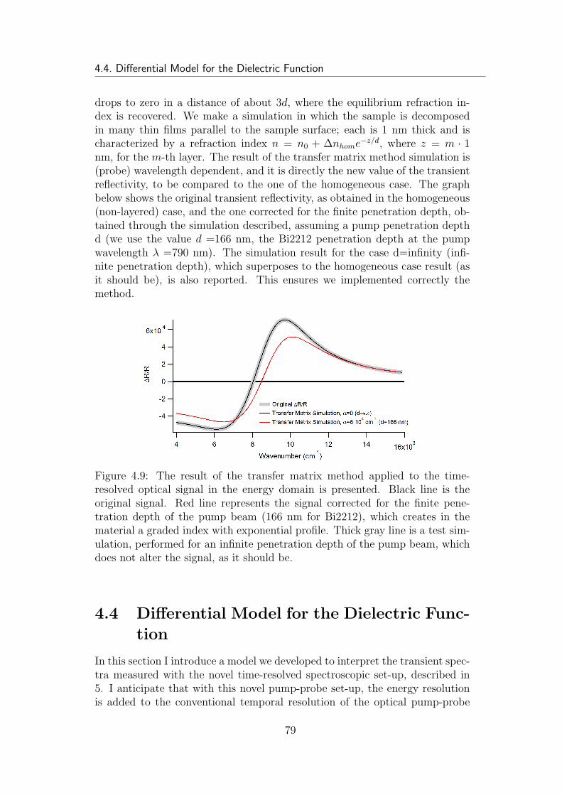
4.4. Differential Model for the Dielectric Function
drops to zero in a distance of about 3d, where the equilibrium refraction in-dex is recovered. We make a simulation in which the sample is decomposedin many thin films parallel to the sample surface; each is 1 nm thick and ischaracterized by a refraction index n = n0 + ∆nhome
−z/d, where z = m · 1nm, for the m-th layer. The result of the transfer matrix method simulation is(probe) wavelength dependent, and it is directly the new value of the transientreflectivity, to be compared to the one of the homogeneous case. The graphbelow shows the original transient reflectivity, as obtained in the homogeneous(non-layered) case, and the one corrected for the finite penetration depth, ob-tained through the simulation described, assuming a pump penetration depthd (we use the value d =166 nm, the Bi2212 penetration depth at the pumpwavelength λ =790 nm). The simulation result for the case d=infinity (infi-nite penetration depth), which superposes to the homogeneous case result (asit should be), is also reported. This ensures we implemented correctly themethod.
Figure 4.9: The result of the transfer matrix method applied to the time-resolved optical signal in the energy domain is presented. Black line is theoriginal signal. Red line represents the signal corrected for the finite pene-tration depth of the pump beam (166 nm for Bi2212), which creates in thematerial a graded index with exponential profile. Thick gray line is a test sim-ulation, performed for an infinite penetration depth of the pump beam, whichdoes not alter the signal, as it should be.
4.4 Differential Model for the Dielectric Func-
tion
In this section I introduce a model we developed to interpret the transient spec-tra measured with the novel time-resolved spectroscopic set-up, described in5. I anticipate that with this novel pump-probe set-up, the energy resolutionis added to the conventional temporal resolution of the optical pump-probe
79
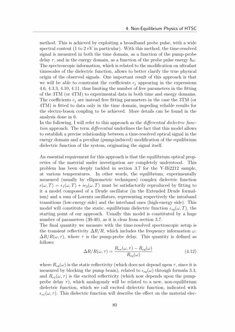
4. Non-Equilibrium Physics of HTSC
method. This is achieved by exploiting a broadband probe pulse, with a widespectral content (1 to 2 eV in particular). With this method, the time-resolvedsignal is measured in both the time domain, as a function of the pump-probedelay τ , and in the energy domain, as a function of the probe pulse energy ~ω.The spectroscopic information, which is related to the modification on ultrafasttimescales of the dielectric function, allows to better clarify the true physicalorigin of the observed signals. One important result of this approach is thatwe will be able to constraint the coefficients cj appearing in the expressions4.6, 4.3.3, 4.10, 4.11, thus limiting the number of free parameters in the fittingof the 3TM (or 4TM) to experimental data in both time and energy domains.The coefficients cj are instead free fitting parameters in the case the 3TM (or4TM) is fitted to data only in the time domain, impeding reliable results forthe electro-boson coupling to be achieved. More details can be found in theanalysis done in 6.In the following, I will refer to this approach as the differential dielectric func-tion approach. The term differential underlines the fact that this model allowsto establish a precise relationship between a time-resolved optical signal in theenergy domain and a peculiar (pump-induced) modification of the equilibriumdielectric function of the system, originating the signal itself.
An essential requirement for this approach is that the equilibrium optical prop-erties of the material under investigation are completely understood. Thisproblem has been deeply tackled in section 3.7 for the Y-Bi2212 sample,at various temperatures. In other words, the equilibrium, experimentallymeasured (usually by ellipsometric techniques) complex dielectric functionǫ(ω, T ) = ǫ1(ω, T ) + iǫ2(ω, T ) must be satisfactorily reproduced by fitting toit a model composed of a Drude oscillator (in the Extended Drude formal-ism) and a sum of Lorentz oscillators, representing respectively the intrabandtransitions (low-energy side) and the interband ones (high-energy side). Thismodel will constitute the static, equilibrium dielectric function ǫeq(ω, T ), thestarting point of our approach. Usually this model is constituted by a hugenumber of parameters (30-40), as it is clear from section 3.7.The final quantity we measure with the time-resolved spectroscopic setup isthe transient reflectivity ∆R/R, which includes the frequency information ω:∆R/R(ω, τ), where τ is the pump-probe delay. This quantity is defined asfollows:
∆R/R(ω, τ) =Rex(ω, τ)−Req(ω)
Req(ω)(4.12)
where Req(ω) is the static reflectivity (which does not depend upon τ , since it ismeasured by blocking the pump beam), related to ǫeq(ω) through formula 3.3,and Rex(ω, τ) is the excited reflectivity (which now depends upon the pump-probe delay τ), which analogously will be related to a new, non-equilibriumdielectric function, which we call excited dielectric function, indicated withǫex(ω, τ). This dielectric function will describe the effect on the material elec-
80
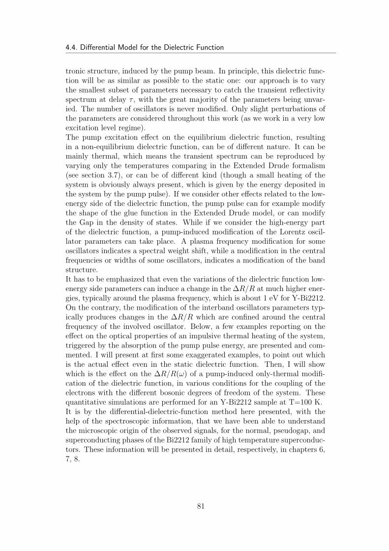
4.4. Differential Model for the Dielectric Function
tronic structure, induced by the pump beam. In principle, this dielectric func-tion will be as similar as possible to the static one: our approach is to varythe smallest subset of parameters necessary to catch the transient reflectivityspectrum at delay τ , with the great majority of the parameters being unvar-ied. The number of oscillators is never modified. Only slight perturbations ofthe parameters are considered throughout this work (as we work in a very lowexcitation level regime).The pump excitation effect on the equilibrium dielectric function, resultingin a non-equilibrium dielectric function, can be of different nature. It can bemainly thermal, which means the transient spectrum can be reproduced byvarying only the temperatures comparing in the Extended Drude formalism(see section 3.7), or can be of different kind (though a small heating of thesystem is obviously always present, which is given by the energy deposited inthe system by the pump pulse). If we consider other effects related to the low-energy side of the dielectric function, the pump pulse can for example modifythe shape of the glue function in the Extended Drude model, or can modifythe Gap in the density of states. While if we consider the high-energy partof the dielectric function, a pump-induced modification of the Lorentz oscil-lator parameters can take place. A plasma frequency modification for someoscillators indicates a spectral weight shift, while a modification in the centralfrequencies or widths of some oscillators, indicates a modification of the bandstructure.It has to be emphasized that even the variations of the dielectric function low-energy side parameters can induce a change in the ∆R/R at much higher ener-gies, typically around the plasma frequency, which is about 1 eV for Y-Bi2212.On the contrary, the modification of the interband oscillators parameters typ-ically produces changes in the ∆R/R which are confined around the centralfrequency of the involved oscillator. Below, a few examples reporting on theeffect on the optical properties of an impulsive thermal heating of the system,triggered by the absorption of the pump pulse energy, are presented and com-mented. I will present at first some exaggerated examples, to point out whichis the actual effect even in the static dielectric function. Then, I will showwhich is the effect on the ∆R/R(ω) of a pump-induced only-thermal modifi-cation of the dielectric function, in various conditions for the coupling of theelectrons with the different bosonic degrees of freedom of the system. Thesequantitative simulations are performed for an Y-Bi2212 sample at T=100 K.It is by the differential-dielectric-function method here presented, with thehelp of the spectroscopic information, that we have been able to understandthe microscopic origin of the observed signals, for the normal, pseudogap, andsuperconducting phases of the Bi2212 family of high temperature superconduc-tors. These information will be presented in detail, respectively, in chapters 6,7, 8.
81
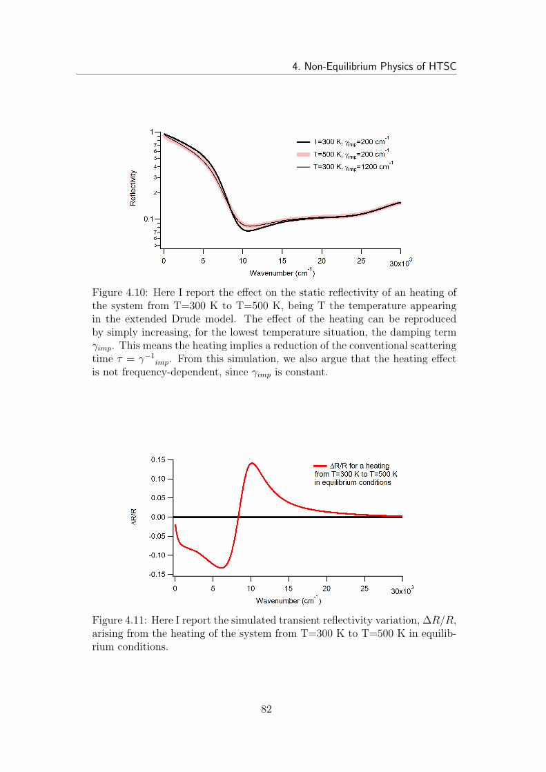
4. Non-Equilibrium Physics of HTSC
Figure 4.10: Here I report the effect on the static reflectivity of an heating ofthe system from T=300 K to T=500 K, being T the temperature appearingin the extended Drude model. The effect of the heating can be reproducedby simply increasing, for the lowest temperature situation, the damping termγimp. This means the heating implies a reduction of the conventional scatteringtime τ = γ−1
imp. From this simulation, we also argue that the heating effectis not frequency-dependent, since γimp is constant.
Figure 4.11: Here I report the simulated transient reflectivity variation, ∆R/R,arising from the heating of the system from T=300 K to T=500 K in equilib-rium conditions.
82
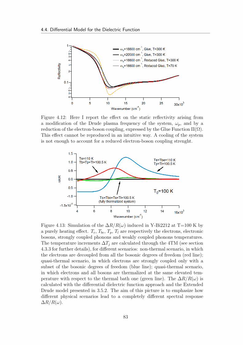
4.4. Differential Model for the Dielectric Function
Figure 4.12: Here I report the effect on the static reflectivity arising froma modification of the Drude plasma frequency of the system, ωp, and by areduction of the electron-boson coupling, expressed by the Glue Function Π(Ω).This effect cannot be reproduced in an intuitive way. A cooling of the systemis not enough to account for a reduced electron-boson coupling strenght.
Figure 4.13: Simulation of the ∆R/R(ω) induced in Y-Bi2212 at T=100 K bya purely heating effect. Te, Tbe, Tp, Tl are respectively the electrons, electronicbosons, strongly coupled phonons and weakly coupled phonons temperatures.The temperature increments ∆Tj are calculated through the 4TM (see section4.3.3 for further details), for different scenarios: non-thermal scenario, in whichthe electrons are decoupled from all the bosonic degrees of freedom (red line);quasi-thermal scenario, in which electrons are strongly coupled only with asubset of the bosonic degrees of freedom (blue line); quasi-thermal scenario,in which electrons and all bosons are thermalized at the same elevated tem-perature with respect to the thermal bath one (green line). The ∆R/R(ω) iscalculated with the differential dielectric function approach and the ExtendedDrude model presented in 3.5.2. The aim of this picture is to emphasize howdifferent physical scenarios lead to a completely different spectral response∆R/R(ω).
83

4. Non-Equilibrium Physics of HTSC
84
Chapter 5Time-Resolved Spectroscopy
5.1 Introduction
The novel results presented in this thesis work have been made possible by anovel experimental technique, the time-resolved optical spectroscopy. Thistechnique constitutes the natural extension of the conventional (one-color)time-resolved ultrafast pump probe technique, in which the spectral (energy)resolution is added to the intrinsic temporal resolution of the technique (∼100fs). In this way, an effective spectroscopy with temporal resolution is achieved.This chapter, after a brief introduction to the time-resolved methods, describesin detail the techniques developed in this work to obtain the spectral resolu-tion. I can anticipate that I fulfilled this task in two complementary ways:exploiting a white-light supercontinuum pulse to cover the visible region ofthe electromagnetic spectrum (1.2-2.2 eV, i.e., 1050-550 nm, i.e., 9500-18000cm−1), and a tunable infrared pulse (obtained through an optical parametricamplifier, OPA), to cover the infrared part of the spectrum (0.5-1.1 eV, i.e.,2450-1100 nm, i.e., 4000-9000 cm−1).
5.2 Motivations
The pump-probe approach is today declined in a wide field of time-resolvedmeasurements, well beyond time-resolved optics. In the pump-probe frame-work, two synchronized pulses are employed. One is the so-called pump beam,exciting in a non-equilibrium condition the sample, while the other is the so-called probe beam, used to measure, as a function of the time delay withrespect to the former, the effect produced by the excitation on one quantityof interest. The first time-resolved experiments, made possible by the adventof pulsed laser sources, were in the field of optics. In these all-optical pump-probe experiments, both the pump and the probe beams are ultrashort (∼100fs) laser pulses, typically in the near-IR region. They are quasi-monochromatic,in the sense that their bandwidth is typically the minimum required by the
85
5. Time-Resolved Spectroscopy
indeterminacy principle for the pulse to be ultrashort (∼10 nm for a ∼100fs, 800 nm pulse). With all-optical pump-probe measurements, the probedquantities are the optical properties of the sample, namely, the reflectivity Ror the transmissivity T . On the contrary to the pump beam, which is oftenthe fundamental of the laser source, soon became clear how a different probecould provide new advances. Considering an all-optical pump-probe, the tun-ability of the optical probe is possible since long time. Usually it is achievedthanks to light-conversion devices, known as Optical Parametric Amplifiers(OPA, see section 5.6). In this way, the spectral range that can be probed isconsiderably widened (the 200-20000 µm range can be explored). However, thenon-equilibrium optical properties can be probed singularly, one-wavelength ata time. Moreover, such light conversion devices work only in combination withhigh-power laser sources, which are not well suited to perform experiments onfragile materials. However, more recently it was demonstrated that the probecan be tuned in the far-IR or THz (1 THz ∼ 4.1 meV) spectral range withconventional, low power sources. This opened the access to the probing of thenon-equilibrium optical properties in the infrared spectral range. As an ex-ample of application of these techniques to probe the non-equilibrium opticalproperties of cuprate superconductors, I may cite, respectively for mid-IR andTHz: [101, 100, 102, 20, 19] and [12, 99]. The study of the evolution of the op-tical properties, simultaneously in a wide range of energies, is a possibility thatonly very recently is encountering an increasing interest. This is made possi-ble thanks to the so-called supercontinuum pulses, i.e., very broadband, whitelight pulses, which energy content can exceed 1 eV. Joining the spectral res-olution to the time-resolved approach considerably helps in the interpretationof the observed non-equilibrium dynamics. Applications of this technique tostrongly correlated electronic materials have been recently reported [82, 169].The problem is that in general such pulses require high-power sources (seesection 5.6) to be generated, and are again not well suited to investigate fromthe non-equilibrium point of view materials which ground state can be easilyaltered, quenched or vaporized by an excitation.
Only recently it has become possible to generate supercontinuum pulses by us-ing low-energy laser sources, thanks to the use of Photonic Crystal Fibers (seesection 5.7 for further details). In this thesis, I developed a set-up exploitingthis new possibility. The important result has been that a novel pump-probesystem allowing to measure simultaneously the temporal evolution of the time-resolved optical signal in a wide range of energies has been developed. Thissetup, on the contrary to the ones based on high-power laser sources, is char-acterized by an enhanced sensibility, and allows to probe the non-equilibriumoptical response of a material which is only slightly brought out of its equilib-rium condition. This ensures the ground state of the system is not stronglyperturbed, with the measured optical response accounting for the typical exci-tations of the ground state itself. This setup constitutes the perfect match for
86
5.3. Time-resolved basics: background, sources, useful definitions and beam
diagnostic
materials which ground state is a phase which free energy only slightly differsfrom the one of the other allowed phases. This is the case of superconductors ormaterials exhibiting charge density wave or spin density wave ordering. Thesephases are vaporized for extremely low values of pump fluence [168].In particular, the spectral resolution combined with the temporal one allowsto understand the physical origin, i.e., on the microscopic level, which origi-nated the non-equilibrium optical signal. This is often precluded to conven-tional time-resolved measurements, probing the time-resolved optical signalat a fixed wavelength. This can be understood by the observation that thespectral resolution allows to interpret the non-equilibrium optical signal bydifferential models applied to the sample dielectric function. By doing so, be-ing the dielectric function related to the electronic structure and the allowedoptical transitions of the material, a close correspondence can be establishedbetween a non-equilibrium signal in the energy domain and one excitation-induced effect on the material electronic structure.It is for this reason that we call this novel experimental technique the time-resolved spectroscopy. It is a spectroscopy, since the spectral resolution hasbeen achieved. It is non-equilibrium, with the peculiarity that the weakly-excited states can be probed, providing information precluded to static spec-troscopy, that only the joined spectral and temporal resolutions can provide.The access to the dynamics, from which the effects related to the thermalheating can be disentangled from the purely electronic ones, and the fact thatthe ground state of the system is not sensibly affected, make this techniquethe ideal tool to probe the strongly correlated electronic materials, in which aninterplay of different phenomena dominate the non-equilibrium optical signal.
For completeness, I must remember that in the last few years the pump-probeapproach has been successfully applied also to non-all-optical techniques. Timeresolved photoemission and time-resolved electron diffraction are widespread-ing techniques. The former technique allows to measure the temporal evolutionof the electronic structure, while the latter allows to study the temporal evo-lution of the crystal structure, after the sample is brought out-of-equilibriumby the absorption of a pump pulse. In both situations, the pump pulse excit-ing the sample is an optical, laser pulse, while the probe pulse is respectivelya high-energy photon (&6 eV) photoemitting electrons or an electron bunchwhich diffraction pattern from the sample is recorded. Examples of applicationof these techniques on cuprates are respectively: [145, 41] and [27].
5.3 Time-resolved basics: background, sources,
useful definitions and beam diagnostic
It is a long time that time-resolved optical measurements are being carriedon on solid state systems. The first examples of such kind of measurements,
87
5. Time-Resolved Spectroscopy
that allowed to study the transient, non equilibrium (optical) properties ofsolid state systems on very short timescales (ps and fs), are dated 1980−1990[165, 63, 64, 163, 25, 24, 87].The key-element for this kind of study is an ultrafast laser system capable ofproducing a train of ultrashort pulses, with a temporal duration of 100-1000fs. Other important parameters of the laser light pulses are their photon en-ergy (or wavelength) and the number of pulses per unit of time (this quantityis known as repetition rate of the source, measured in Hz). For Ti:Sapphiresources, that is, the most common laser systems today available for researchpurposes, the pulse photon energy equals 1.55 eV (i.e. 800 nm, 12500 cm−1);this is called the fundamental of the laser. Ti:Sapphire, i.e., Ti doped Al2O3,is the active medium inserted in the laser cavity.The majority of time-resolved measurements published up to now, are per-formed by using the fundamental energy (or its harmonics: 2nd - 3.14 eV(400 nm); 3rd - 4.51 eV (266 nm), 4th - 6.28 eV (200 nm)) to measure thetransient optical properties. This is what we call conventional (or one-color)pump-probe measurements. This approach, although capable of revealing thenon-equilibrium dynamics of a system on a timescale (< 1 ps) not accessibleto other non-optical techniques, has an important limit: the dynamics canbe measured at a single and fixed energy. This prevents, in most situations,the understanding of the microscopic origin of the (differential) time-resolvedoptical signal. To achieve this ambitious goal, the range of energies for whichthe non-equilibrium dynamics of a system is measured, must be widened. Thisopens the way to the knowledge of the non-equilibrium dielectric function ofa system, from which a great amount of information can be, in general, ex-tracted. The realization of this target will be described in detail in the nextsections of this chapter.
Laser sources classificationThe average power at the output of a standard laser system is of the orderof some (1-4) Watts. Depending on the repetition rate of the source, threeclasses of lasers can be distinguished today. The key parameter is the energyper pulse, measured in J.
• The so-called oscillators produce train of pulses at 80-100 MHz: thisresults in an energy per pulse of the order 5-50 nJ/pulse. This sourcecan be coupled to an acousto-optic device to control the repetition rateof the source, from some MHz to single-pulse. This device is called pulse-picker (if it is placed outside the cavity) or cavity-dumper (if it is placedinside the cavity, resulting in a minor amount of losses). Both thesedevices are useful in reducing the average thermal heating of the sampleunder study. This is mandatory in the field of low-temperature physics.
• The regenerative-class of laser systems have repetition rate tunable from
88
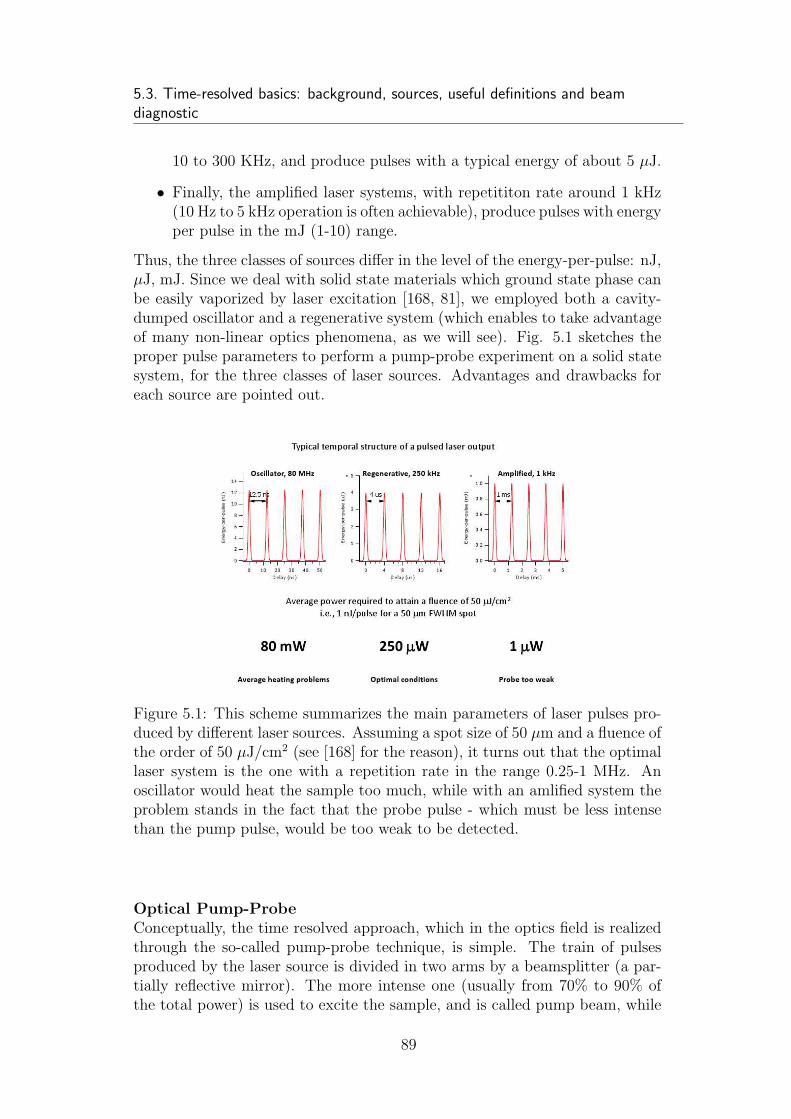
5.3. Time-resolved basics: background, sources, useful definitions and beam
diagnostic
10 to 300 KHz, and produce pulses with a typical energy of about 5 µJ.
• Finally, the amplified laser systems, with repetititon rate around 1 kHz(10 Hz to 5 kHz operation is often achievable), produce pulses with energyper pulse in the mJ (1-10) range.
Thus, the three classes of sources differ in the level of the energy-per-pulse: nJ,µJ, mJ. Since we deal with solid state materials which ground state phase canbe easily vaporized by laser excitation [168, 81], we employed both a cavity-dumped oscillator and a regenerative system (which enables to take advantageof many non-linear optics phenomena, as we will see). Fig. 5.1 sketches theproper pulse parameters to perform a pump-probe experiment on a solid statesystem, for the three classes of laser sources. Advantages and drawbacks foreach source are pointed out.
Figure 5.1: This scheme summarizes the main parameters of laser pulses pro-duced by different laser sources. Assuming a spot size of 50 µm and a fluence ofthe order of 50 µJ/cm2 (see [168] for the reason), it turns out that the optimallaser system is the one with a repetition rate in the range 0.25-1 MHz. Anoscillator would heat the sample too much, while with an amlified system theproblem stands in the fact that the probe pulse - which must be less intensethan the pump pulse, would be too weak to be detected.
Optical Pump-ProbeConceptually, the time resolved approach, which in the optics field is realizedthrough the so-called pump-probe technique, is simple. The train of pulsesproduced by the laser source is divided in two arms by a beamsplitter (a par-tially reflective mirror). The more intense one (usually from 70% to 90% ofthe total power) is used to excite the sample, and is called pump beam, while
89
5. Time-Resolved Spectroscopy
the less intense one (10% to 30% of the total power) is employed to measurethe pump-induced change in the optical properties of the sample, and is calledprobe beam.By optical properties I mean the reflectivity R of the sample, or its transmis-sivity T (if the sample is transparent to the actual probe wavelength), or both.Thus, the probe beam reflected or transmitted from the sample, is collectedwith a sensing element (usually a photodiode) and the generated electric sig-nal is acquired and digitized. On the contrary, the pump beam is dumped.In the time-resolved approach, the relative change (transient) in the opticalproperties is measured. This means that the measured quantity is the rela-tive variation induced by the pump. In a typical time-resolved experiment,the measured quantity is the difference between the reflectivity Rpumped of theexcited (pumped) system and the reflectivity Runpumped of the equilibrium (un-pumped) system, divided by the equilibrium reflectivity, that is:
∆R
R(ω, τ) =
Rpumped(ω, τ)−Runpumped(ω)
Runpumped(ω)(5.1)
τ is the actual delay between the pump and probe beams; expression 5.1, inprinciple, also depends on ω, the frequency of the probe photon energy ~ω.The ∆R/R(ω, τ) is usually very small with respect to the values Rpumped andRunpumped. In practice, R is the reflected light intensity from the sample, andnot the true reflectivity. However, since, as it is always the case, the incidentintensity I0 on the sample is unchanged, R has the same meaning of the ac-tual reflectivity, in the ∆R/R expression. The same argument holds for thetransmissivity T. Both the quantities ∆R/R and ∆T/T have the advantage ofbeing universal, i.e., independent (as far as one works in a linear regime) fromthe incident probe intensity I0. Usually, ∆R/R ranges from 10−2 to 10−6. Thismeans that the detection system, described subsequently, must be very accu-rate. It must have a dynamic range able to reveal signal variations as smallas one part over one million, ie, ∼1 µV, if the total ligth intensity produces asignal R∼1 V on the detector. The detection system must be characterized bya signal-to-noise ratio (S/N) higher than the 1/(∆R/R) induced by the pumppulse.
Pump-probe delay, τIn expression 5.1, τ is the time delay between the arrival of the pump andprobe pulses on the sample. It is of the order of tens of fs, and, if one wantsto exploit the full temporal resolution of the system, it is of the same order ofthe pulse duration. The time resolution, as small as the laser pulse duration,comes from the fact that the ultrashort probe laser pulses sample the reflectiv-ity or the transmissivity of the sample, ’integrating’ it on a time window equalto that of the pulse duration.The delay τ is varied, to study the dynamics of the system, simply changingthe relative length of the optical path of the pump and the probe arms. This
90
5.3. Time-resolved basics: background, sources, useful definitions and beam
diagnostic
is achieved with a mechanical delay stage or with a coil, on which a coupleof mirrors (to reflect the beam) are mounted. One µm of displacement intro-duces a delay equal to 6.66 fs between the pump and probe beams (1µm · 3.33fs/µm · 2, where the 2 comes from the doubling of the path upon reflection).
Time-resolved optical traceTo measure a pump-probe trace (a plot of the ∆R/R or ∆T/T for a numberof pump-probe delays τ), two types of approach are possible.The first consists in acquiring the ∆R/R signal point-by-point, modifying therelative delay and subsequently acquiring the signal, for a time long enough toobtain the desired noise level in the measurement (usually, 1 s signal averageper point is enough to obtain a S/N of the order 105, for a ∼1 MHz repetitionrate source).The second approach consists in scanning quickly the delay between pump andprobe, and acquiring continuously and synchronously the ∆R/R signal. Thetemporal windows of the acquisition should be kept as small as possible not tolower the temporal resolution, thus, to lower the noise in the measurements,many scans are needed, which must then be averaged. Usually, 100-1000 scansare enough to obtain a S/N of the order 105, for a ∼1 MHz repetition ratesource. This method (called ’fast scan’) requires a fast (and with the lowestpossible inertia) delay stage. This approach constitutes a clear advantage be-cause, since every scan is completed on a time of the order of 1 s, it helpssuppressing the disturbing effects related to the laser source fluctuations andthe effects of the sample degradation (when the sample is placed inside a cryo-stat, for example). The drawback is that the delay stages designed for thistask have a short travel range, and the amount of data to acquire is huge, thusthis approach is limited to small ranges of delay (of the order of 10-50 ps). Ifone needs to explore a wider range of delays (this depends on the dynamicsone wants to analyze), the point-to-point approach is the only one that can beexploited. The speed (in mm/s, or ps/s, if one converts the displacement indelay) of the delay stage, vD, and the acquisition time window tW of the ac-quisition system set the temporal resolution of the measurements according tothe following formula: Resolution(ps)=vD(ps/s)·tW (s). This quantity is oftenlarger than the limit resolution given by the pulse duration, in the case of fslaser; what it is important is that this quantity must be smaller than the dy-namics one wants to measure. Some numbers are helpful: if vD=10 ps/s∼1.5mm/s for the delay stage, and the acquisition time window tW is set to 1 ms,the maximum achievable temporal resolution is 10 fs. If a 10 ps pump-probescan is required, each scan would take 2 s (2·1 s, since the delay stage must goback and forth).
Direct digitization of the signal vs Lock-in acquisition
91
5. Time-Resolved Spectroscopy
The acquisition of the signal must be done taking in mind that very often,extremely small variations in the signal (less than one µV) must be detected.The direct digitalization of the photodiode electric signal is thus a poor ideain the great majority of the experiments. This would require very high reso-lution digitizers (> 16 bit: over a 1 V full-scale, 16 bit means ∼15 µV, whichis too much in many cases), which are rare and expensive. This approach isalso very sensitive to the various sources of electrical noise. Anyway, to obtaina differential signal, the procedure is to acquire the reflected signal R with(’pumped’) and without (’unpumped’) the pump beam, and performing thedifference with the correct parity (which must be sensed in some way). Themost common way to modulate the pump status is to make use of a so-calledoptical chopper, a device constituted by a disk with a mask of regular holes(designed in such a way to achieve a 50% duty cycle for the modulation), whichis put in rotation by a high speed motor. The laser beam is thus chopped bythe disk at a frequency ranging from ∼1 Hz to ∼100 kHz (with a proper choiceof the disk mesh).The Lock-In amplifier solves the resolution problems coming from a directdigitization of the signal. By using a complex algorithm based on Fouriertransforms, multiplications and filtering of the signal, carried on by a fast DSP(digital signal processor), this device can extract, from an electric signal ofhigh intensity, only a component which has a frequency equal to that fed inby an external reference. If one modulates the pump beam with a chopper(whose frequency reference is brought to the lock-in), and the pumping hasan effect on the optical properties of the system, detected with a photodiode,connected to the lock-in input, the lock-in output will be only - and directly- the pump induced variation of the optical properties, ∆R. To obtain thequantity ∆R/R, the static signal R must be sampled in some way. This is aminor problem, since R is of the order of 1 V. The advantage of this approachis that all sources of noise (with frequency different from the chopper one)are intrinsically suppressed. In general, the higher the chopper frequency f ,the lower the noise level ∝ 1/
√f , for the noise related to the acquisition sys-
tem. In the case of lock-in acquisition, the acquisition time window tW definedabout the fast scan method equals the lock-in integration time. The chopperfrequency must be higher (10 times or more) than t−1
W .
Temporal and Spatial superpositionTo perform a pump-probe experiment, the temporal and spatial coincidenceconditions, for the pump and probe beams on the sample, must be achieved.The condition for which pump and probe impinges simultaneously on the sam-ple is called temporal coincidence. This means that the pump and probe armshave the same optical length, and thus this particular delay τ is defined τ0 = 0.Often, but not always, at this particular delay one observes the maximum vari-ation of the optical properties.
92
5.3. Time-resolved basics: background, sources, useful definitions and beam
diagnostic
For what concern the spatial coincidence condition, the maximum of the time-resolved optical signal is achieved when the probe beam is exactly at the centerof the (pump) excited area. To make the measure more reliable, usually thepump spot on the sample is kept larger than the probe spot, and this is ob-tained by focusing the pump beam on the sample with a lens with focal lengthbigger than the focal length of the lens on the probe beam. This ensures thatthe probe probes an area which is uniformly excited. The spatial superpositionof the beams on the sample is checked with a CCD camera, equipped with anobjective collecting the light scattered by the sample.To avoid interference effects on the sample, usually the pump and probe beampolarizations are kept orthogonal. This helps also to prevent that the pumplight scattered by the sample reaches the detector, simply placing a polarizerin front of it. Another solution to improve the measurements quality is toplace the delay stage on the pump path: the fact that the pump spot is bigger,and that the pump should not be collected, drastically reduces the effect ofmisalignments, that would produce non-physical variations in the signal.
5.3.1 Beam Parameters
Key parameters that must be known in order to correctly set up a measure-ment and interpret the acquired data are the spot size and the pulse duration,for both the pump and the probe beams, on the sample. Typically, laser pulsesare Gaussian both in space and in time. They remain Gaussian up to the sam-ple, if they are properly propagated.
Spot lateral sizeTwo methods can be employed to measure the spot size. The first consistssimply in measuring the intensity profile of the beam itself, when impinging ona scattering material placed at the sample position. This task is achieved byimaging the spot on a CCD (Charge-Coupled-Device) camera. To have a goodresolution, since typical spot sizes are of the order of 20-50 µm and the CCDpixel size is of the order of 5 µm, a magnifying objective is often used. Then,a Gaussian profile is fitted to the image, along various directions, to extractthe beam size.The second method is called ’the knife-edge’. The position of a knife, mountedon a precision translation stage, is scanned perpendicularly through the beam,in the same position where the sample would be. By means of a photodiode, thetotal transmitted intensity is acquired, as a function of the knife position. Thisintensity equals the integral along one axis (defined by the direction of move-ment of the knife) of the product of the Gaussian pulse intensity, multipliedby a step function expressing the knife position. The integral of a Gaussianfunction can thus be fitted to the acquired trace, to extract the actual spot
93
5. Time-Resolved Spectroscopy
size. In this work, the spot lateral size equals the spot FWHM (Full-Width-at-Half-Maximum).
Pulse temporal widthThe temporal duration of ultrashort laser pulses can be measured by acquiringtheir sum frequency intensity [93], generated in a non linear crystal (usuallyBBO, beta-barium borate) placed at the sample position, as a function of thepump-probe delay τ . Sum frequency generation (SFG) is a non-linear processinvolving the energy mixing of two photons [93]. If pulses are Gaussian intime, their sum frequency signal is Gaussian too. Mathematically, the SFGprocess is expressed as a convolution of the intensities Ij(t) of the two pulses:
C(τ) =∫ +∞
−∞Ipump(t)Iprobe(t− τ)dt, being C(τ) the sum-frequency signal.
If the pump and probe optical paths are different, i.e., contain a differentnumber of dispersing optical devices, only the pulses cross-correlation can bedetermined. The pump-probe cross-correlation sets the lower limit for the tem-poral resolution the system can provide. If the two optical paths are similar,the measure can be approximated to an auto-correlation. Assuming that thepulses are Gaussian, their individual duration is given by their autocorrelationdivided by a deconvolution factor, equal to
√2 for Gaussian pulses [84].
The cross- (or auto-) correlation sum-frequency signal versus the pump-probedelay τ contains the information of the pulse duration. In practice, to extractthis information, a Gaussian function is fitted to the sum-frequency signal.In this work, the pump-probe cross-correlation is expressed as the temporalFWHM (Full-Width-at-Half-Maximum) of the correlation signal.
FluenceThe pump fluence is defined as the energy per pulse divided by the area illu-minated by the pump beam spot. It is usually expressed in µJ/cm2. The spotarea is calculated from the pump spot lateral FWHM, which is carefully deter-mined with the methods described above. Indicating the pump fluence is themost common way to express the pump excitation intensity of the system. Theprobe beam fluence should be always kept orders of magnitude weaker thanthe pump one, to avoid further perturbations of the system. Typical valuesfor the pump fluence employed in this work are comprised in the range 1-100µJ/cm2. Working at the lowest fluence values requires some level of care. Aswe will se, some interesting physics is learnt just at this (low) level of excitation(∼10 µJ/cm2), since HTSC are very susceptible to an external perturbation,particularly when they are in the superconducting phase.
Up to now, a general overview on the time-resolved approach has been pro-vided. Anyway, the details of the various optical setups employed are describedin the subsequent sections of this same chapter. For what concerns one-colormeasurements, a basic experimental system requires no more components than
94
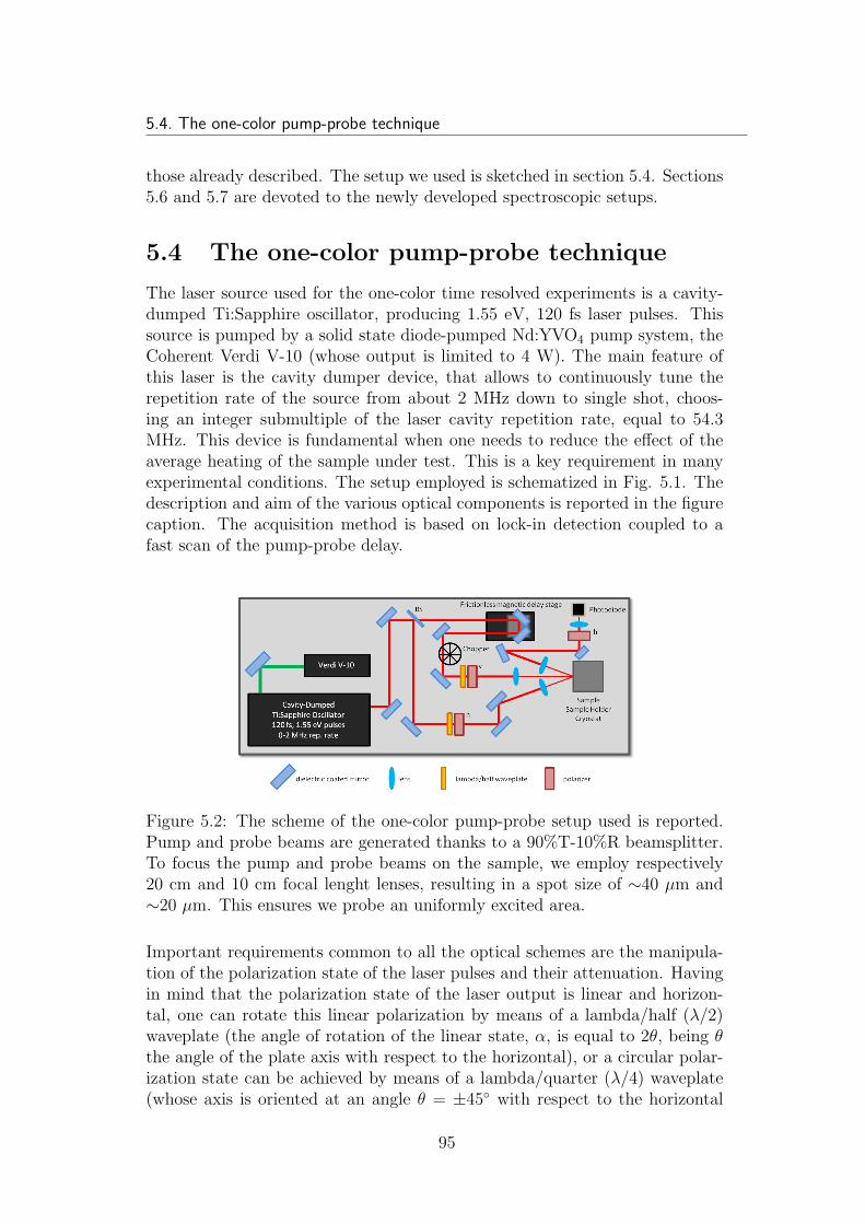
5.4. The one-color pump-probe technique
those already described. The setup we used is sketched in section 5.4. Sections5.6 and 5.7 are devoted to the newly developed spectroscopic setups.
5.4 The one-color pump-probe technique
The laser source used for the one-color time resolved experiments is a cavity-dumped Ti:Sapphire oscillator, producing 1.55 eV, 120 fs laser pulses. Thissource is pumped by a solid state diode-pumped Nd:YVO4 pump system, theCoherent Verdi V-10 (whose output is limited to 4 W). The main feature ofthis laser is the cavity dumper device, that allows to continuously tune therepetition rate of the source from about 2 MHz down to single shot, choos-ing an integer submultiple of the laser cavity repetition rate, equal to 54.3MHz. This device is fundamental when one needs to reduce the effect of theaverage heating of the sample under test. This is a key requirement in manyexperimental conditions. The setup employed is schematized in Fig. 5.1. Thedescription and aim of the various optical components is reported in the figurecaption. The acquisition method is based on lock-in detection coupled to afast scan of the pump-probe delay.
Figure 5.2: The scheme of the one-color pump-probe setup used is reported.Pump and probe beams are generated thanks to a 90%T-10%R beamsplitter.To focus the pump and probe beams on the sample, we employ respectively20 cm and 10 cm focal lenght lenses, resulting in a spot size of ∼40 µm and∼20 µm. This ensures we probe an uniformly excited area.
Important requirements common to all the optical schemes are the manipula-tion of the polarization state of the laser pulses and their attenuation. Havingin mind that the polarization state of the laser output is linear and horizon-tal, one can rotate this linear polarization by means of a lambda/half (λ/2)waveplate (the angle of rotation of the linear state, α, is equal to 2θ, being θthe angle of the plate axis with respect to the horizontal), or a circular polar-ization state can be achieved by means of a lambda/quarter (λ/4) waveplate(whose axis is oriented at an angle θ = ±45 with respect to the horizontal
95
5. Time-Resolved Spectroscopy
line). In our setups, for both the pump and the probe beams, we employ lin-early polarized fields. The possibility to rotate the relative polarizations of thepump and the probe beams is important since it allows to investigate possibleanisotropies in the optical response or in the excitation process. To attenuatea (linearly polarized) laser beam, a lambda/half waveplate plus a polarizer isused. The output polarization is linear, and parallel to the polarizer axis. Theoutput intensity, if the input polarization and the polarizer axis are horizontal,and theta is the same as before, is: I = I0(cos
2(θ) − sin2(θ))2, being I0 theincident intensity. The optical components are often designed to work at asingle wavelength, but broadband components (which work in a wide range ofwavlenghts) also exist.
5.5 Toward the time resolved spectroscopy
So far, I described the pump and probe approach for conventional one-colour(probe) measurements, with the details of the optical layout we employed forthis kind of measurements (Fig. 5.1), and I defined some common importantconcepts which are universal in the field of time-resolved optics. As I anticipate,the novelty of this thesis is to extend this approach to a configuration in whichthe probe is no more a monochromatic pulse, but rather a broadband pulsewhich contains a continuum of wavelengths (supercontinuum), or it is a quasi-monochromatic pulse which can be continuously tuned across a wide rangeof energies. This allowed us to achieve time-resolved spectroscopy, i.e., tocombine the temporal resolution with the spectral one. The time-resolvedsignal of expression 5.1 is indeed wavelength dependent, and this additionalinformation opens the way to a new physics, adding a ’dimension’ (the energyresolution) in our measurements. This new dimension finally allowed us toassign a clear physical origin to the measured transient signals, as reported inChapters 6, 7, 8.The two different approaches we followed are described in this chapter, startingfrom the tunable probe configuration, which is a straightforward evolution ofthe single-color setup. Finally, a comment about the excitation (pump beam)role. In the work reported here, the pump photon-energy is fixed, and equalto 1.55 eV (i.e., 800 nm). A systematic study of the effects of the excitationphoton-energy tuning on the transient optical properties is beyond the scopeof this work. However, we checked that the results were independent on thepump photon energy, repeating the most meaningful measurements with aSHG pumping. Despite this, a systematic study of the excitation mechanismcould reveal some interesting features.
96
5.6. Tunable-Probe Pump-Probe Setup
5.6 Tunable-Probe Pump-Probe Setup
The pump-probe setup described in this section was designed to perform time-resolved measurements with a probe energy in the near infrared region of theelectromagnetic spectrum. In particular, the probe energy can be continuouslytuned in the range 1100-2450 nm (i.e., 1.1-0.5 eV, 9000-4000 cm−1). The pumpis kept fixed at the fundamental energy value of 1.55 eV.While the details of the optical setup are similar to those described in Fig.5.1, what it is different is the laser source. The conversion of a 1.55 eV beaminto a (tunable) infrared beam requires to exploit a non linear phenomenon,called parametric amplification. The device which allows to do this is calledoptical parametric amplifier, also known as OPA. These non linear phenomenarequires energy per pulse of the order of µJ/pulse, thus a regenerative lasersource must be employed.Our laser source is the Coherent RegA 9050 system, a Ti:Sapphire laser systempumped by a Verdi V-18 solid state laser (producing 18W of monochromaticCW (continuous wave) radiation at 532 nm). The final laser output consistsof a train of 1.55 eV, 50 fs laser pulses. The repetition rate of this sourcecan be continuously tuned from 10 to 300 kHz. At a 250 kHz repetition rate,the one we used, the output power is about 1.5 W. This gives an energy perpulse of about 6 µJ. Very briefly, the scheme of this complex laser system isas follows: the 532 nm output (18 W) of the Verdi diode-pumped Nd:YVO4
pump system is splitted in two parts: ∼6 W are brought to a Ti:Sapphireoptical oscillator (Mira Seed), while the remaining ∼12 W are borught to theregenerative cavity (RegA). The oscillator produces a train of <100 fs, 1.55eV pulses, with a fixed repetition rate of 80 MHz. These pulses are fed in astretcher, a device based on diffraction gratings which aim is to increase thetemporal duration of the laser pulses. These pulses are the seed pulses to beamplified by the regenerative cavity, in which they are fed in after having beentemporally-stretched. In the regenerative multi-pass cavity the amplificationprocess takes place. This process happens because the seed pulses pass througha Ti:Sapphire active medium for a proper number of times (20 to 30), until thedesired energy has been reached for the pulse. The injection of the seed pulsein the cavity and the ejection of the amplified pulse are both obtained withan acousto-optic device (a cavity dumper). This device is a SiO2 cell, whoseindex of refraction is modulated by a strain wave induced by a piezoelectric el-ement, driven by a proper radiofrequency, in such a way that the beam passingthrough the cell is diffracted when the radiofrequency is applied. A complexelectronics synchronizes the timing of the injection with the 80 MHz pulse trainof Mira Seed, and manage the injection and ejection phases of the radiofre-quency for the acousto-optic device. The seed pulses and the amplified pulses,which propagate collinearly, are separated thanks to a faraday rotator coupledto a polarizer. The amplified pulse is then recompressed with a grating-basedcompressor. The seed pulse must be stretched before the amplification, other-wise the peak intensity would be too high for a good amplification process to
97
5. Time-Resolved Spectroscopy
occur. Obviously, not all the seed pulses are amplified: the RegA repetitionrate is a sub-multiple of the seed laser repetition rate; the actual seed pulse tobe amplified is picked by the cavity dumper, the others are dumped.The 70% of the laser system output is fed to the OPA, for wavelength con-version. The resulting energy per pulse is of the order of 4 uJ. The remaining30% is employed for the pump in pump-probe experiments. The Optical Para-metric Amplifier is the Coherent OPA 9850. Its output consists in two beams,called signal and idler, whose energy can be continuously varied in a specifiedrange. The infrared (1100-1600 nm) part of a white-light supercontinuum,generated focusing 25% of the total power in a Sapphire plate, is amplifiedin phase-matching conditions in a Type II BBO nonlinear crystal, exploitinga two-pass cavity design. The pump beam used for the amplification processis the remaining 75% of the total power entering the OPA. Two aspects areworth to be described in more detail: the supercontinuum generation and theamplification process itself. The supercontinuum generation is achieved in a 2mm thick Sapphire plate, on which is focused (with a short focal lenght (30mm) lens) an energy of about 1 µJ/pulse. In this way, a stable supercontinuumcan be obtained. The generation threshold in Sapphire is about 500 nJ/pulse.Over this threshold, a self-focusing effect, related to the Kerr effect, occurs,and the intensity-dependent index of refraction of the material, being the in-coming pulse spatially Gaussian, behaves like a lens for the pulse itself. Thus,extremely high pulse intensity develops, and various non linear phenomena co-operate to broaden the spectral content of the seed pulse. The most importantnon linear phenomena is the self phase modulation. The amplification processtakes place in a 1 mm thick BBO non linear crystal. This process in calledparametric amplification, and involves three beams (photons). In this process,the energy and momentum conservation relations, for the three photons, aresatisfied simultaneously. These three beams / photons are: the seed beam,the one which will be amplified, and which comes from the supercontinuum:this will be the signal, s; the pump beam, which will be depleted after theamplification, indicated with p, and the idler, i, which is generated to matchthe energy and momentum conservation relations. ωj and kj are respectivelythe angular frequencies and momenta of the three beams. The energy andmomentum conservation relations write:
ωi = ωp − ωs
ωp = ωs + ωi
ki = kp − ks
The second expression indicates that one pump photon is annihilated, and twonew photons, the signal and the idler, whose energy sum equals the pumpone, are generated. There is thus a transfer of energy from the pump, whichwill be depleted, to the signal and the idler. The seed pulse coming from thesupercontinuum ’tells’ the system which frequency will be amplified. If the
98
5.6. Tunable-Probe Pump-Probe Setup
axis orientation for the crystal matches the momentum conservation relationbetween the pump and the seed beams (this implies the so-called phase match-ing condition is satisfied), a good amplification efficiency is achieved. Startingfrom the sub-nJ energy level of the seed, a mean energy of more than 400nJ/pulse is obtained for the signal, in a two step amplification process in thesame BBO crystal.Being 1.55 eV, 800 nm the energy of the pump beam, the degeneracy conditionfor the amplification process will be that for which both the signal and the idlerhave the same energy of 0.75 eV, 1600 nm. The signal output is comprised inthe interval from 1100 to 1600 nm, while the idler output ranges from 2450to 1600 nm. They are generated in a collinear geometry, and thus are bothpresent at the OPA output. Signal and Idler have (linear) orthogonal polariza-tions, thus they can be alternatively selected with a polarizer. The energies ofthe couple of produced signal and idler can be tuned continuously in the rangeindicated. Once aligned, the tuning of the device is quite simple. It consists inthe modification of the phase matching angle of the non-linear crystal, and inthe compensation of the delays between the pump and the seed or signal, forboth the two amplification steps. The signal and idler pulse duration has beencharacterized with a cross correlation with a 50 fs 800 nm pulse, when the OPAis seeded with a 50 fs pulse. The result is that the average pulse duration is ofabout 100 fs. Now that the laser radiation sources have been described, a briefdescription of the optical layout used to carry the experiments is provided. Aschematic of the optical layout is presented in Fig. 5.3. In this configuration,the pump and the probe beams reach the optic bench being already divided.The pump beam comes directly from the RegA output, while the probe beamcomes from the OPA output: it is either the signal or the idler pulse. In thisway, the probe pulse can be tuned continuously from 1100 to 2450 nm. Toswitch from signal to idler, a polarizer is used, which is rotated by 90 degressto select the signal (horizontal) or the idler (vertical). To ensure the polariza-tion of the two is the same on the sample, a broadband lambda/half waveplateplus a second polarizer (kept fixed) is employed. To compensate for the opticalpath of the OPA (about 5 m), the pump path is lengthened exploiting the re-flection from some retroreflectors. The probe pulse must be attenuated by anamount of 100 to 10000 (with a neutral density filter with optical density (OD)continuously variable from 2 to 4) to ensure it is weak enough to be employedas a probing beam. To introduce a carefully variable time delay between pumpand probe beams, the pump beam is brought to a retroreflector mounted on acoil motor. This device (APE ScanDelay 50) is computer controlled and allowsto introduce a delay ranging from 10 to 50 ps in the beam path. Its motionequals a triangular wave, with a rise-time tunable from 0.1 to 5 s. This meansthat a complete pump-probe scan can be acquired in a time ranging from 0.2 to10 s (5 to 0.1 Hz rate). This device is designed to allow acquisitions in the ’fastscan’ configuration I described in section 5.2. We set the relevant parametersas follows: for a 10 ps scan, a rise time of 0.2 s was chosen. With a lock-in
99
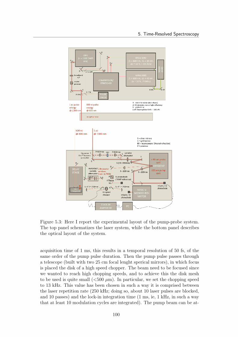
5. Time-Resolved Spectroscopy
Figure 5.3: Here I report the experimental layout of the pump-probe system.The top panel schematizes the laser system, while the bottom panel describesthe optical layout of the system.
acquisition time of 1 ms, this results in a temporal resolution of 50 fs, of thesame order of the pump pulse duration. Then the pump pulse passes througha telescope (built with two 25 cm focal lenght sperical mirrors), in which focusis placed the disk of a high speed chopper. The beam need to be focused sincewe wanted to reach high chopping speeds, and to achieve this the disk meshto be used is quite small (<500 µm). In particular, we set the chopping speedto 13 kHz. This value has been chosen in such a way it is comprised betweenthe laser repetition rate (250 kHz; doing so, about 10 laser pulses are blocked,and 10 passes) and the lock-in integration time (1 ms, ie, 1 kHz, in such a waythat at least 10 modulation cycles are integrated). The pump beam can be at-
100
5.7. Supercontinuum-Probe Pump-Probe Setup
tenuated with a computer controlled lambda/half waveplate, placed behind apolarizer made of two Brewster angle windows. In this way, the measurementscan be automatically repeated at various values of excitation intensity. Finally,the pump beam is focused on the sample with an anti-reflection coated 40 cmfocal length lens. The probe path is much simpler: no particular devices areneeded, and the beam is focused with a 25 cm focal length spherical mirror.The choice of a spherical mirror has been done since this optical componentis achromatic (the probe can range from 1100 to 2450 nm). This ensures theprobe spot size is almost constant in the entire spectral range. We obtained100±5 um for the pump FWHM and 50±5 um for the probe FWHM, at thesample position. The reflected or transmitted beam from the sample is imagedonto pin photodiodes of the InGaAs type. Two photodiode types (which differin the doping of the sensing area) help to cover the whole probe energy range.They are Thorlabs DET10C and DET10D, which detect light respectively inthe 700-1800 nm and 1200-2600 nm range. Placed in front of the photodiode,an RG 1000 filter blocks the scattered light coming from the 1.55 eV pumpbeam. The detection system is based on a lock-in acquisition. This allows usto reach a signal to noise level as high as 106, averaging about 200 scans (last-ing 0.4 s each). To obtain the ∆R/R signal, the static quantity R is measuredaveraging the photodiode signal over 10 ms windows, and sampling them witha 16 bit-100 kHz digitizer. The same digitizer acquires the analog X and Yfast outputs of the lock-in amplifier, from which is calculated the ∆R signal,and the position signal coming from the ScanDelay. To obtain a plot of the∆R/R signal at the different probe wavelengths, the OPA must be manuallytuned. This procedure requires some time (everything must be kept aligned),so that a complete ∆R/R map requires some hours to be collected (consideringa pump fluence of ∼100 µJ and 20 lambda-points).
5.7 Supercontinuum-Probe Pump-Probe Setup
In this setup the spectral resolution enters in a natural way, since the probepulse is itself a broadband pulse, with a wide energy content. No need tomanually tune the probe wavelength is necessary anymore, which often resultsin misalignment problems. The main difference with respect to the setups de-scribed till now, stands in the acquisition system. Here, the spectral signal, ata fixed pump-probe delay, is acquired simultaneously in a wide spectral range,thanks to a multichannel linear detector (a linear array of photodiodes onwhich the spectrum is dispersed) which is digitized using an analog-to-digitalacquisition board. No lock-in detection is possible in this setup, and this re-sults in a poorer signal-to-noise ratio with respect to lock-in based acquisitions.But since no dead time dedicated to tuning and realignment is spent, the fi-nal result is similar: the acquisition of the transient time-resolved spectra atdifferent pump-probe delays can be repeated many times in a fully automatedway. With respect to the tunable-probe approach, the ∆R/R 2D map is con-
101
5. Time-Resolved Spectroscopy
structed following a different ’filling’: transient spectra at a fixed pump-probedelay (which is then scanned in the point-by-point configuration) are collected.On the contrary, different time-resolved traces at fixed wavelength (to be man-ually tuned) were collected in the previous approach. In our case, the lineararray sensors have 128 pixels: this implies that the spectral resolution is muchhigher than the previous approach, and also narrow spectral features can bedetected.
After a brief description of the optical system and the acquisition system wedeveloped for this task, particular importance will be devoted to the char-acterization methods for the broadband supercontinuum pulses. The nextparagraph of this chapter will be entirely devoted to this aim. A brief de-scription of the mechanisms which produce the white light continuum startingfrom a monochromatic seed pulse, will reveal that the temporal structure ofthese pulses can be far from trivial. Since the temporal structure of the probepulse reflects itself in a pump probe spectrally resolved scan, for the data to becorrectly interpreted and presented, the temporal structure of the pulse (thetemporal distribution of the various wavelengths) must be a priori character-ized. In this way, the raw data can be corrected from the unphysical featuresrelated uniquely to the probe temporal structure. Thus, a review of sometechniques we developed and employed to obtain the supercontinuum pulsespectrograms (time and energy maps of the pulse) will be presented, evidenc-ing pros and cons of each technique.
A supercontinuum pulse can be generated following two different approaches.As a common starting point, an ultrashort (∼100 fs) monochromatic laserpulse must be focalized in a medium, in such a way that very high peak inten-sities are reached. Depending on the material one chooses, the initial energyper pulse must belong to a completely different energy range. In the case ofbulk materials (such as Sapphire, CaF2, BBO) or liquids (water, ethanol), thethreshold for supercontinuum generation is of the order of ∼500 µJ/cm2. Fol-lowing this approach, the first broadening of a monochromatic ultrashort pulsewas demonstrated [3, 4] in 1970. The temporal structure of these pulses is ingeneral quite simple: the various wavelengths have a linear and positive chirp,related to that of the material in which the generation occurs. To generate asupercontinuum following this approach, one needs an amplified laser system,which is a rather complex and expensive machine. On the contrary, super-continuum pulses can be generated starting from pulses with a much lowerenergy per pulse, of the order of some nJ/pulse, if one exploits the recentlydeveloped photonic crystal fibers (PCF). The first report on a PCF-generatedsupercontinuum is dated 2000 [152, 107, 158, 61]. Following this approach, su-percontinuum pulses can be generated using a standard oscillator laser source.The drawback is that the temporal structure of these pulses is more compli-cated, and must be known in some way prior to use these pulses as probe
102
5.7. Supercontinuum-Probe Pump-Probe Setup
pulses in time-resolved experiments. The temporal structure is involved be-cause it follows the effective dispersion characteristic of the fiber, and becauseof the various physical phenomena which contributes to the broadening of thespectrum. From now on, for dispersion characteristic I mean the behavior ofthe group velocity dispersion (GVD) versus the radiation wavelength.
A few words about the PCFs are worth to be spent. An optical fiber is con-stituted by two concentric materials: the internal one, named core, in whichthe light is guided, and the external one, the cladding. The most common ma-terial for both the constituent is fused silica. The light propagation throughan optical fiber is made possible by the phenomenon of the total internal re-flection: this phenomenon confines the light inside the material with higherrefraction index (the core), since the reflectivity at the interface is one if theincident angle θi is bigger enough (it must be bigger than the critical angleθc, that is θi > θc = arcsin(ncl/nc), being nc and ncl the refraction index ofthe core and the cladding, respectively). This condition is easily satisfied for abeam propagating inside an optical fiber. In a conventional optical fiber, the(wavelength dependent) refraction index of the core is made bigger than thatof the cladding, upon a proper doping of the material. The problem is that thedispersion characteristic of the fiber will be the same of the material, and thismakes the conventional optical fibers not well suited to the production of super-continuum: a short pulse temporally broadens and thus cannot non-linearlyinteract with the fiber core material (for fused silica, zero dispersion occursclose to 1.5 µm). On the contrary, the dispersion characteristic of photoniccrystal fibers is designed in such a way the dispersion is zero close to the seedwavelength (which is usually 800 nm, the fundamentalof Ti:Sapphire lasers).Doing so, the (ultrashort) seed pulse remains short upon propagation in thefiber, and the high peak intensities make it non-linearly interact with the core.The desired dispersion characteristic for the a PCF is obtained (see Fig. 5.4)thanks to a microstructured cladding, which is usually composed of a regular(computer designed) pattern of holes which surround the core. This peculiardesign results in an effective refraction index, for the cladding, which is smallerthan the core one, with the advantage that the dispersion characteristic canbe enginerized as one needs. From the cladding enginerized structure, whichresembles that of some crystals, the photonic crystal fibers take their name.Many non linear phenomena, which take place in the fiber core, contribute andcooperate to the broadening of the monochromatic (800 nm) seed pulse intoa broadband white light supercontinuum pulse. These phenomena are: theself phase modulation, the Raman scattering, the four wave mixing and thesolitonic fission. The last is specific to the light propagation in optical fibers.For a detailed description of these phenomena I suggest Ref. [61]. Since manyphysically different phenomena participate in the spectral broadening of theseed pulse, the pulse temporal structure will be rather involved, and difficultto be predicted. Anyway, the pulse temporal structure will closely follow the
103
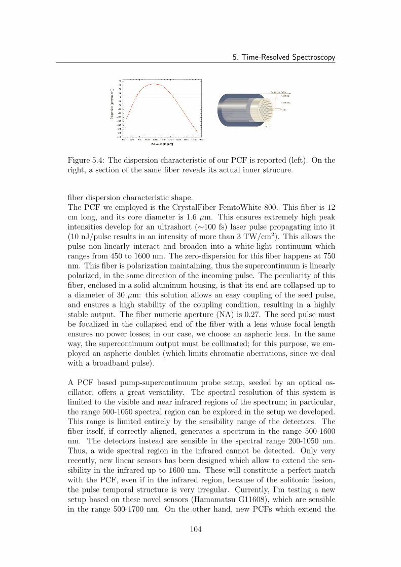
5. Time-Resolved Spectroscopy
Figure 5.4: The dispersion characteristic of our PCF is reported (left). On theright, a section of the same fiber reveals its actual inner strucure.
fiber dispersion characteristic shape.The PCF we employed is the CrystalFiber FemtoWhite 800. This fiber is 12cm long, and its core diameter is 1.6 µm. This ensures extremely high peakintensities develop for an ultrashort (∼100 fs) laser pulse propagating into it(10 nJ/pulse results in an intensity of more than 3 TW/cm2). This allows thepulse non-linearly interact and broaden into a white-light continuum whichranges from 450 to 1600 nm. The zero-dispersion for this fiber happens at 750nm. This fiber is polarization maintaining, thus the supercontinuum is linearlypolarized, in the same direction of the incoming pulse. The peculiarity of thisfiber, enclosed in a solid aluminum housing, is that its end are collapsed up toa diameter of 30 µm: this solution allows an easy coupling of the seed pulse,and ensures a high stability of the coupling condition, resulting in a highlystable output. The fiber numeric aperture (NA) is 0.27. The seed pulse mustbe focalized in the collapsed end of the fiber with a lens whose focal lengthensures no power losses; in our case, we choose an aspheric lens. In the sameway, the supercontinuum output must be collimated; for this purpose, we em-ployed an aspheric doublet (which limits chromatic aberrations, since we dealwith a broadband pulse).
A PCF based pump-supercontinuum probe setup, seeded by an optical os-cillator, offers a great versatility. The spectral resolution of this system islimited to the visible and near infrared regions of the spectrum; in particular,the range 500-1050 spectral region can be explored in the setup we developed.This range is limited entirely by the sensibility range of the detectors. Thefiber itself, if correctly aligned, generates a spectrum in the range 500-1600nm. The detectors instead are sensible in the spectral range 200-1050 nm.Thus, a wide spectral region in the infrared cannot be detected. Only veryrecently, new linear sensors has been designed which allow to extend the sen-sibility in the infrared up to 1600 nm. These will constitute a perfect matchwith the PCF, even if in the infrared region, because of the solitonic fission,the pulse temporal structure is very irregular. Currently, I’m testing a newsetup based on these novel sensors (Hamamatsu G11608), which are sensiblein the range 500-1700 nm. On the other hand, new PCFs which extend the
104
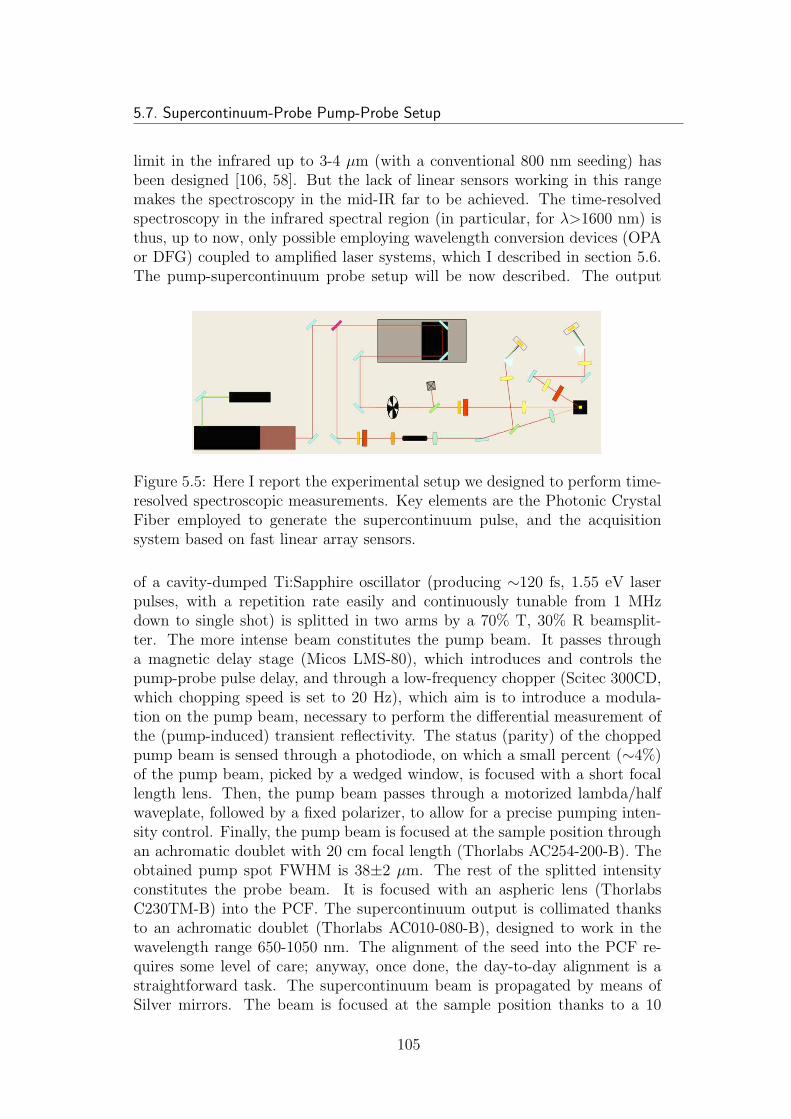
5.7. Supercontinuum-Probe Pump-Probe Setup
limit in the infrared up to 3-4 µm (with a conventional 800 nm seeding) hasbeen designed [106, 58]. But the lack of linear sensors working in this rangemakes the spectroscopy in the mid-IR far to be achieved. The time-resolvedspectroscopy in the infrared spectral region (in particular, for λ>1600 nm) isthus, up to now, only possible employing wavelength conversion devices (OPAor DFG) coupled to amplified laser systems, which I described in section 5.6.The pump-supercontinuum probe setup will be now described. The output
Figure 5.5: Here I report the experimental setup we designed to perform time-resolved spectroscopic measurements. Key elements are the Photonic CrystalFiber employed to generate the supercontinuum pulse, and the acquisitionsystem based on fast linear array sensors.
of a cavity-dumped Ti:Sapphire oscillator (producing ∼120 fs, 1.55 eV laserpulses, with a repetition rate easily and continuously tunable from 1 MHzdown to single shot) is splitted in two arms by a 70% T, 30% R beamsplit-ter. The more intense beam constitutes the pump beam. It passes througha magnetic delay stage (Micos LMS-80), which introduces and controls thepump-probe pulse delay, and through a low-frequency chopper (Scitec 300CD,which chopping speed is set to 20 Hz), which aim is to introduce a modula-tion on the pump beam, necessary to perform the differential measurement ofthe (pump-induced) transient reflectivity. The status (parity) of the choppedpump beam is sensed through a photodiode, on which a small percent (∼4%)of the pump beam, picked by a wedged window, is focused with a short focallength lens. Then, the pump beam passes through a motorized lambda/halfwaveplate, followed by a fixed polarizer, to allow for a precise pumping inten-sity control. Finally, the pump beam is focused at the sample position throughan achromatic doublet with 20 cm focal length (Thorlabs AC254-200-B). Theobtained pump spot FWHM is 38±2 µm. The rest of the splitted intensityconstitutes the probe beam. It is focused with an aspheric lens (ThorlabsC230TM-B) into the PCF. The supercontinuum output is collimated thanksto an achromatic doublet (Thorlabs AC010-080-B), designed to work in thewavelength range 650-1050 nm. The alignment of the seed into the PCF re-quires some level of care; anyway, once done, the day-to-day alignment is astraightforward task. The supercontinuum beam is propagated by means ofSilver mirrors. The beam is focused at the sample position thanks to a 10
105
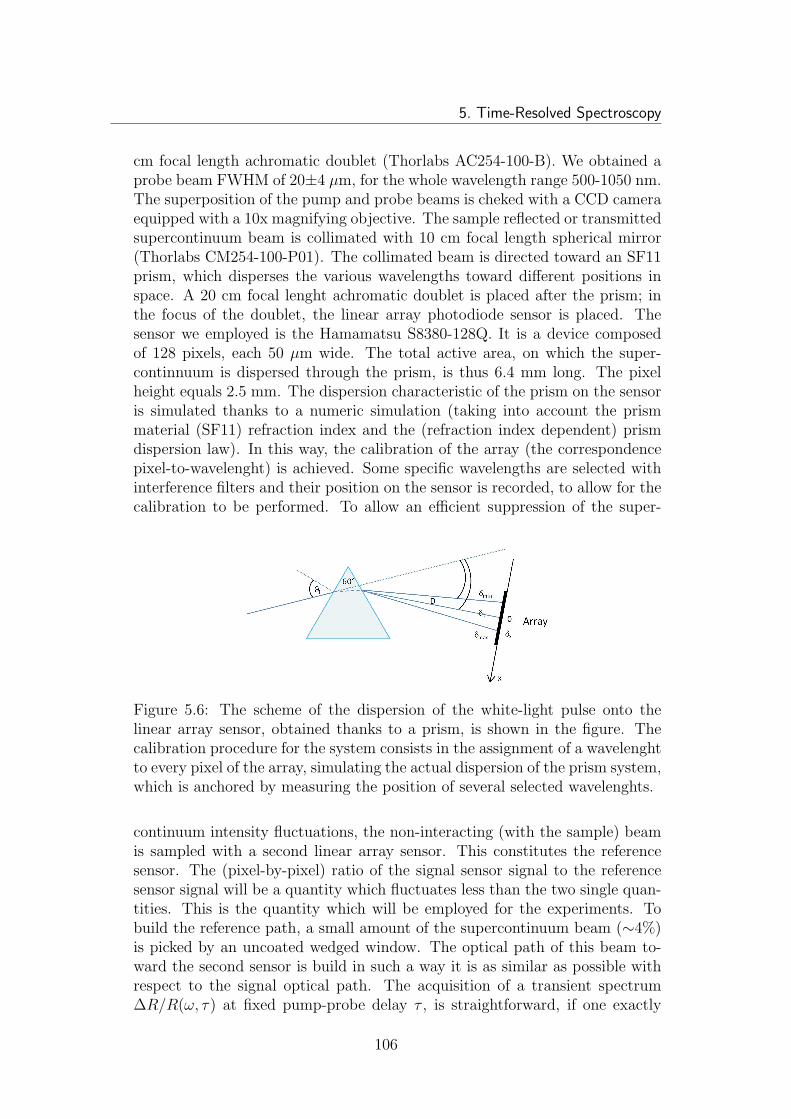
5. Time-Resolved Spectroscopy
cm focal length achromatic doublet (Thorlabs AC254-100-B). We obtained aprobe beam FWHM of 20±4 µm, for the whole wavelength range 500-1050 nm.The superposition of the pump and probe beams is cheked with a CCD cameraequipped with a 10x magnifying objective. The sample reflected or transmittedsupercontinuum beam is collimated with 10 cm focal length spherical mirror(Thorlabs CM254-100-P01). The collimated beam is directed toward an SF11prism, which disperses the various wavelengths toward different positions inspace. A 20 cm focal lenght achromatic doublet is placed after the prism; inthe focus of the doublet, the linear array photodiode sensor is placed. Thesensor we employed is the Hamamatsu S8380-128Q. It is a device composedof 128 pixels, each 50 µm wide. The total active area, on which the super-continnuum is dispersed through the prism, is thus 6.4 mm long. The pixelheight equals 2.5 mm. The dispersion characteristic of the prism on the sensoris simulated thanks to a numeric simulation (taking into account the prismmaterial (SF11) refraction index and the (refraction index dependent) prismdispersion law). In this way, the calibration of the array (the correspondencepixel-to-wavelenght) is achieved. Some specific wavelengths are selected withinterference filters and their position on the sensor is recorded, to allow for thecalibration to be performed. To allow an efficient suppression of the super-
Figure 5.6: The scheme of the dispersion of the white-light pulse onto thelinear array sensor, obtained thanks to a prism, is shown in the figure. Thecalibration procedure for the system consists in the assignment of a wavelenghtto every pixel of the array, simulating the actual dispersion of the prism system,which is anchored by measuring the position of several selected wavelenghts.
continuum intensity fluctuations, the non-interacting (with the sample) beamis sampled with a second linear array sensor. This constitutes the referencesensor. The (pixel-by-pixel) ratio of the signal sensor signal to the referencesensor signal will be a quantity which fluctuates less than the two single quan-tities. This is the quantity which will be employed for the experiments. Tobuild the reference path, a small amount of the supercontinuum beam (∼4%)is picked by an uncoated wedged window. The optical path of this beam to-ward the second sensor is build in such a way it is as similar as possible withrespect to the signal optical path. The acquisition of a transient spectrum∆R/R(ω, τ) at fixed pump-probe delay τ , is straightforward, if one exactly
106
5.7. Supercontinuum-Probe Pump-Probe Setup
knows the pump parity. To calculate the ∆R/R(ω, τ), the Rpumped(ω, τ) andRun−pumped(ω, τ) = Run−pumped(ω) are the only quantities that must be ac-quired (the ’unpumped’ spectrum does not depend on the pump-probe delay).Usually, for each transient spectrum at fixed pump-probe delay, 2000 spectraare recorded and averaged. This takes about 1 s. Part of these spectra willbe ’pumped’, part ’unpumped’. The pump parity is sampled together withthe spectra, thus the ∆R/R(ω, τ) can be computed. To obtain a time andspectrum resolved map of the material optical response, many transient spec-tra, for different pump-probe delays τ , must be collected. Usually, we recordabout 250 delay points for a 6.6 ps total delay scan, which results in a tem-poral resolution of 26.4 fs. The spectral resolution of this system is about 2nm/pixel toward the visible part of the spectrum (500 nm) and 6 nm/pixeltoward the infrared side (1050 nm). This resolution is not constant because ofthe dispersion characteristic of the prism. Anyway, it is a good value and it isenough to evidence spectral feature in the time-resolved signal. The choice ofa grating to disperse light would have produced a linear dispersion, thus a con-stant resolution (in nm), but at the expense of a much lower intensity efficiency.
A dedicated acquisition system has been developed and constructed to per-form this kind of measurements. No commercial systems for this purpose areavailable yet. The acquisition system is devoted to both the control of thelinear array sensors and the acquisition of their outputs. The software part,developed in a LabVIEW environment, controls the acquisition and saves thetime and energy resolved maps as 2D matrices. I anticipated that no lock-inacquisition is possible with this acquisition scheme. This is due to the sensors,the Hamamatsu S8380-128Q (plus the control electronics C7883), which makeavailable the data in a serial form: the voltage information (proportional tothe illumination level) for the 128 pixels is output on the same electrical lineat a 2 MHz rate (if one drives the devices at 8 MHz), thanks to an integratedshift register circuit. Thus, the data acquisition can be performed solely bydigitizing (in our case with a National Instruments high speed digitizer, theNI PCI-5922, which offers two independent ADCs with 22 bit of resolution ata 2 MHz acquisition rate) the train of voltage values for the 128 pixels. Thislimits the final signal-to-noise ratio to a value slightly better than 104, with anacquisition time of about 1 s. The acquisition is performed simultaneously forboth the sensors, and the pixel-by-pixel ratio of the two voltages is immediatelycomputed. The parity signal for the pump status is acquired with a standardNational Instruments M-Series board, the NI PCIe-6251. The Hamamatsusensors, in order to work, need two control signals: one is an 8 MHz clock,which drives the shift register for the pixel voltage value reading; the other isa lower-frequency signal whose frequency inverse equals the integration timeof the sensor, equal for every pixel. The frequency of this signal has an upperbound, which is 15625 kHz (or 64 µs). This is the value needed to completea scan of the whole array (128 pixels · 0.5 µs/pixel, since the sensors respond
107
5. Time-Resolved Spectroscopy
at a 2 MHz rate when driven with an 8 MHz clock, which is the maximumallowed value). This signal is fed to both the arrays (in addition to the settingof the integration time, it starts the output of the data toward the video line)and to the acquisition boards, for which acts as trigger for the acquisition ofthe data. The acquisition is synchronized to the laser trigger, in such a waythat the same number of pulses is acquired for every spectrum, and a constantillumination level (thus of signal) is generated, independently of the (tunable)laser repetition rate. Since the range of repetition rates we use is comprisedbetween 100 kHz and 1 MHz, the laser trigger must be divided by some integervalue. Single shot acquisition is not possible (it would also result in a signalclose to the background level). After some tests, we conclude that an optimalvalue is 256: this means that every spectrum is the result of the accumulationof 256 laser pulses. With this divider, the laser repetition rate can be as highas 4 MHz for the system to work correctly. Anyway, the maximum repetitionrate one can set is about 1 MHz: the limit is given by the acquisition boards,which cannot handle a trigger event rate of more than some (4-5) kHz. All thedigital timing signals for the sensors and the acquisition boards are generatedby an ad-hoc circuit based on high-speed and low-latency logic gates.
5.8 The characterization of a supercontinuum
pulse
This section is devoted to the presentation of some methods to perform thecharacterization of a supercontinuum light pulse. These methods are recentlyattracting much interest [37, 184], given the growing appeal and diffusionof pump-probe setups with spectral resoluton, in the time-resolved scientificcommunity. Pulse characterization is indeed a fundamental step to performwhether broadband supercontinuum pulses are going to be employed as probepulses in time-resolved pump-probe measurements. In fact, the temporal struc-ture of the probe pulse affects the measurements, and, particularly when thetemporal structure of the pulse is not trivial (as it is the case for PCF gener-ated supercontinuum pulses), a detailed knowledge of the pulse spectral andtemporal intensity distribution (spectrogram) must be obtained, through acareful characterization procedure we present here in detail. The informationextracted from the characterization procedure are enough to correct the mea-surements from the pulse temporal structure, making them pulse-structure-independent as they should be.
The experimental apparatus with which the characterization procedure canbe carried on, is the same as presented before; if needed, the specific differ-ences will be highlighted. A comparison of the advantages and drawbacks foreach method will be also presented.
108
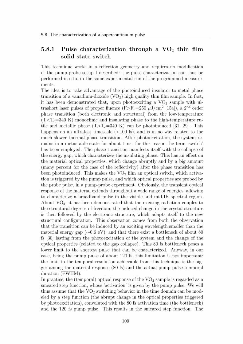
5.8. The characterization of a supercontinuum pulse
5.8.1 Pulse characterization through a VO2 thin filmsolid state switch
This technique works in a reflection geometry and requires no modificationof the pump-probe setup I described: the pulse characterization can thus beperformed in situ, in the same experimental run of the programmed measure-ments.The idea is to take advantage of the photoinduced insulator-to-metal phasetransition of a vanadium-dioxide (VO2) high quality thin film sample. In fact,it has been demonstrated that, upon photoexciting a VO2 sample with ul-trashort laser pulses of proper fluence (F>Fc=250 µJ/cm2 [154]), a 2nd orderphase transition (both electronic and structural) from the low-temperature(T<Tc=340 K) monoclinic and insulating phase to the high-temperature ru-tile and metallic phase (T>Tc=340 K) can be photoinduced [31, 29]. Thishappens on an ultrafast timescale (<100 fs), and is in no way related to themuch slower thermal phase transition. After photoexcitation, the system re-mains in a metastable state for about 1 ns: for this reason the term ’switch’has been employed. The phase transition manifests itself with the collapse ofthe energy gap, which characterizes the insulating phase. This has an effect onthe material optical properties, which change abruptly and by a big amount(many percent for the case of the reflectivity) after the phase transition hasbeen photoinduced. This makes the VO2 film an optical switch, which activa-tion is triggered by the pump pulse, and which optical properties are probed bythe probe pulse, in a pump-probe experiment. Obviously, the transient opticalresponse of the material extends throughout a wide range of energies, allowingto characterize a broadband pulse in the visible and mid-IR spectral region.About VO2, it has been demonstrated that the exciting radiation couples tothe structural degrees of freedom; the induced change in the crystal structureis then followed by the electronic structure, which adapts itself to the newstructural configuration. This observation comes from both the observationthat the transition can be induced by an exciting wavelength smaller than thematerial energy gap (∼0.6 eV), and that there exist a bottleneck of about 80fs [30] lasting from the photoexcitation of the system and the change of theoptical properties (related to the gap collapse). This 80 fs bottleneck poses alower limit to the shortest pulse that can be characterized. Anyway, in ourcase, being the pump pulse of about 120 fs, this limitation is not important:the limit to the temporal resolution achievable from this technique is the big-ger among the material response (80 fs) and the actual pump pulse temporalduration (FWHM).In practice, the (temporal) optical response of the VO2 sample is regarded as asmeared step function, whose ’activation’ is given by the pump pulse. We willthus assume that the VO2 switching behavior in the time domain can be mod-eled by a step function (the abrupt change in the optical properties triggeredby photoexcitation), convoluted with the 80 fs activation time (the bottleneck)and the 120 fs pump pulse. This results in the smeared step function. The
109
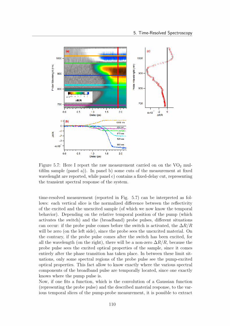
5. Time-Resolved Spectroscopy
Figure 5.7: Here I report the raw measurement carried on on the VO2 mul-tifilm sample (panel a)). In panel b) some cuts of the measurement at fixedwavelenght are reported, while panel c) contains a fixed-delay cut, representingthe transient spectral response of the system.
time-resolved measurement (reported in Fig. 5.7) can be interpreted as fol-lows: each vertical slice is the normalized difference between the reflectivityof the excited and the unexcited sample (of which we now know the temporalbehavior). Depending on the relative temporal position of the pump (whichactivates the switch) and the (broadband) probe pulses, different situationscan occur: if the probe pulse comes before the switch is activated, the ∆R/Rwill be zero (on the left side), since the probe sees the unexcited material. Onthe contrary, if the probe pulse comes after the switch has been excited, forall the wavelength (on the right), there will be a non-zero ∆R/R, because theprobe pulse sees the excited optical properties of the sample, since it comesentirely after the phase transition has taken place. In between these limit sit-uations, only some spectral regions of the probe pulse see the pump-excitedoptical properties. This fact allow to know exactly where the various spectralcomponents of the broadband pulse are temporally located, since one exactlyknows where the pump pulse is.Now, if one fits a function, which is the convolution of a Gaussian function(representing the probe pulse) and the described material response, to the var-ious temporal slices of the pump-probe measurement, it is possible to extract
110
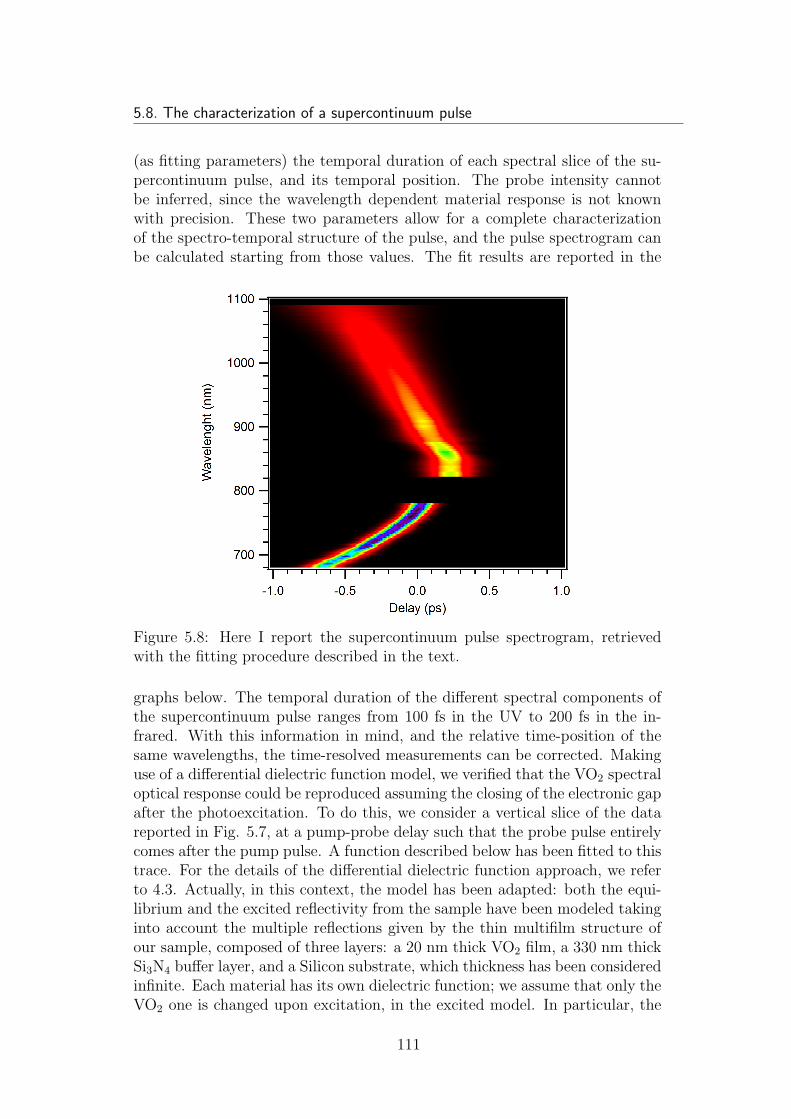
5.8. The characterization of a supercontinuum pulse
(as fitting parameters) the temporal duration of each spectral slice of the su-percontinuum pulse, and its temporal position. The probe intensity cannotbe inferred, since the wavelength dependent material response is not knownwith precision. These two parameters allow for a complete characterizationof the spectro-temporal structure of the pulse, and the pulse spectrogram canbe calculated starting from those values. The fit results are reported in the
Figure 5.8: Here I report the supercontinuum pulse spectrogram, retrievedwith the fitting procedure described in the text.
graphs below. The temporal duration of the different spectral components ofthe supercontinuum pulse ranges from 100 fs in the UV to 200 fs in the in-frared. With this information in mind, and the relative time-position of thesame wavelengths, the time-resolved measurements can be corrected. Makinguse of a differential dielectric function model, we verified that the VO2 spectraloptical response could be reproduced assuming the closing of the electronic gapafter the photoexcitation. To do this, we consider a vertical slice of the datareported in Fig. 5.7, at a pump-probe delay such that the probe pulse entirelycomes after the pump pulse. A function described below has been fitted to thistrace. For the details of the differential dielectric function approach, we referto 4.3. Actually, in this context, the model has been adapted: both the equi-librium and the excited reflectivity from the sample have been modeled takinginto account the multiple reflections given by the thin multifilm structure ofour sample, composed of three layers: a 20 nm thick VO2 film, a 330 nm thickSi3N4 buffer layer, and a Silicon substrate, which thickness has been consideredinfinite. Each material has its own dielectric function; we assume that only theVO2 one is changed upon excitation, in the excited model. In particular, the
111
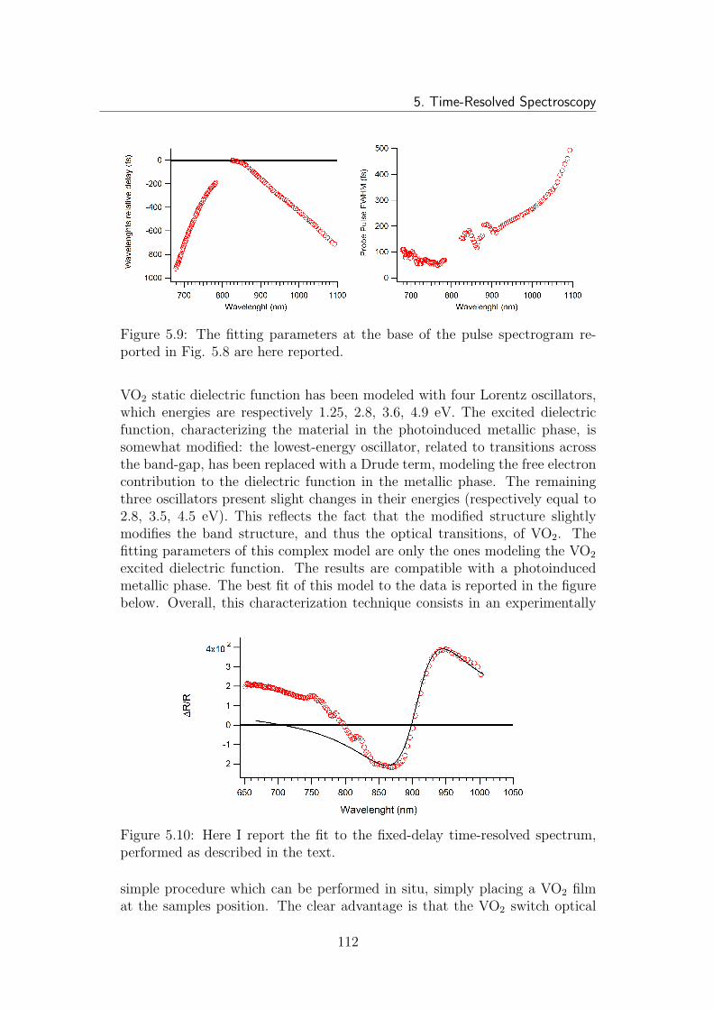
5. Time-Resolved Spectroscopy
Figure 5.9: The fitting parameters at the base of the pulse spectrogram re-ported in Fig. 5.8 are here reported.
VO2 static dielectric function has been modeled with four Lorentz oscillators,which energies are respectively 1.25, 2.8, 3.6, 4.9 eV. The excited dielectricfunction, characterizing the material in the photoinduced metallic phase, issomewhat modified: the lowest-energy oscillator, related to transitions acrossthe band-gap, has been replaced with a Drude term, modeling the free electroncontribution to the dielectric function in the metallic phase. The remainingthree oscillators present slight changes in their energies (respectively equal to2.8, 3.5, 4.5 eV). This reflects the fact that the modified structure slightlymodifies the band structure, and thus the optical transitions, of VO2. Thefitting parameters of this complex model are only the ones modeling the VO2
excited dielectric function. The results are compatible with a photoinducedmetallic phase. The best fit of this model to the data is reported in the figurebelow. Overall, this characterization technique consists in an experimentally
Figure 5.10: Here I report the fit to the fixed-delay time-resolved spectrum,performed as described in the text.
simple procedure which can be performed in situ, simply placing a VO2 filmat the samples position. The clear advantage is that the VO2 switch optical
112
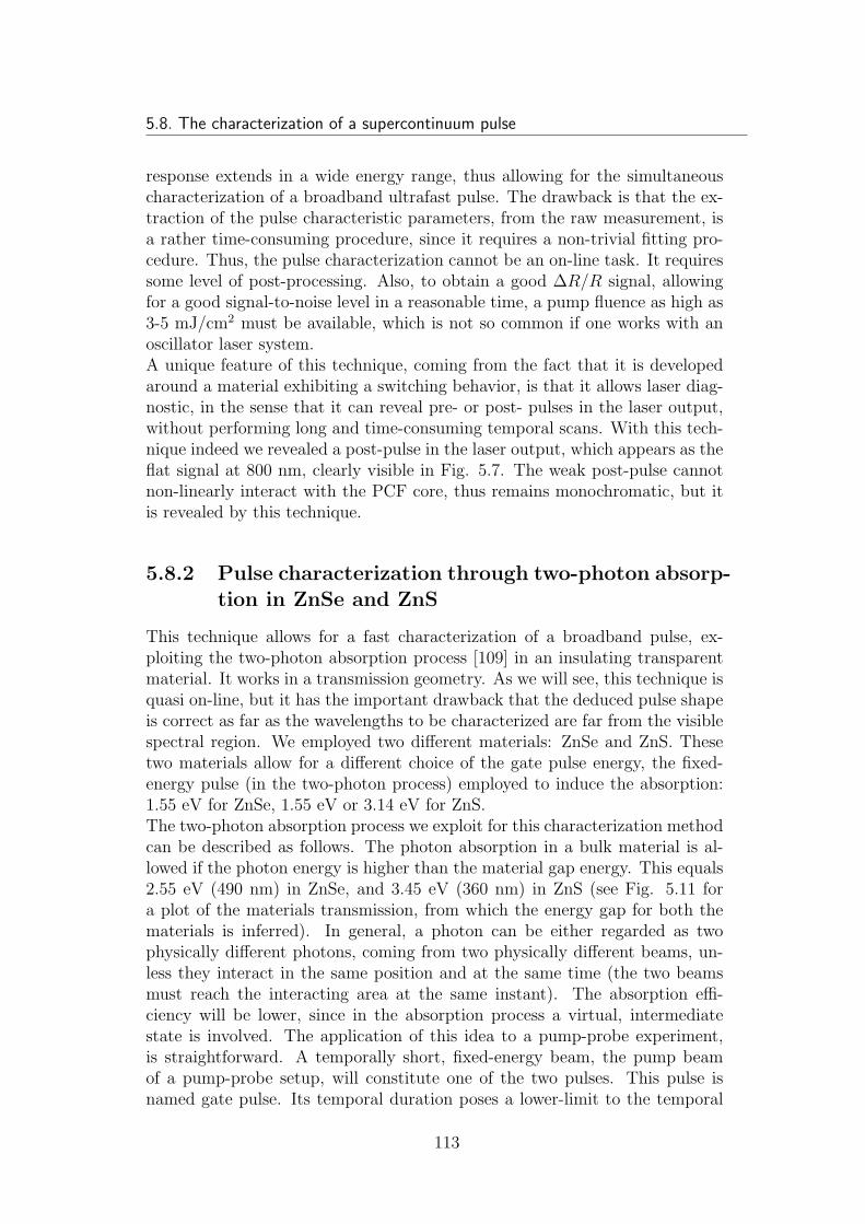
5.8. The characterization of a supercontinuum pulse
response extends in a wide energy range, thus allowing for the simultaneouscharacterization of a broadband ultrafast pulse. The drawback is that the ex-traction of the pulse characteristic parameters, from the raw measurement, isa rather time-consuming procedure, since it requires a non-trivial fitting pro-cedure. Thus, the pulse characterization cannot be an on-line task. It requiressome level of post-processing. Also, to obtain a good ∆R/R signal, allowingfor a good signal-to-noise level in a reasonable time, a pump fluence as high as3-5 mJ/cm2 must be available, which is not so common if one works with anoscillator laser system.A unique feature of this technique, coming from the fact that it is developedaround a material exhibiting a switching behavior, is that it allows laser diag-nostic, in the sense that it can reveal pre- or post- pulses in the laser output,without performing long and time-consuming temporal scans. With this tech-nique indeed we revealed a post-pulse in the laser output, which appears as theflat signal at 800 nm, clearly visible in Fig. 5.7. The weak post-pulse cannotnon-linearly interact with the PCF core, thus remains monochromatic, but itis revealed by this technique.
5.8.2 Pulse characterization through two-photon absorp-tion in ZnSe and ZnS
This technique allows for a fast characterization of a broadband pulse, ex-ploiting the two-photon absorption process [109] in an insulating transparentmaterial. It works in a transmission geometry. As we will see, this technique isquasi on-line, but it has the important drawback that the deduced pulse shapeis correct as far as the wavelengths to be characterized are far from the visiblespectral region. We employed two different materials: ZnSe and ZnS. Thesetwo materials allow for a different choice of the gate pulse energy, the fixed-energy pulse (in the two-photon process) employed to induce the absorption:1.55 eV for ZnSe, 1.55 eV or 3.14 eV for ZnS.The two-photon absorption process we exploit for this characterization methodcan be described as follows. The photon absorption in a bulk material is al-lowed if the photon energy is higher than the material gap energy. This equals2.55 eV (490 nm) in ZnSe, and 3.45 eV (360 nm) in ZnS (see Fig. 5.11 fora plot of the materials transmission, from which the energy gap for both thematerials is inferred). In general, a photon can be either regarded as twophysically different photons, coming from two physically different beams, un-less they interact in the same position and at the same time (the two beamsmust reach the interacting area at the same instant). The absorption effi-ciency will be lower, since in the absorption process a virtual, intermediatestate is involved. The application of this idea to a pump-probe experiment,is straightforward. A temporally short, fixed-energy beam, the pump beamof a pump-probe setup, will constitute one of the two pulses. This pulse isnamed gate pulse. Its temporal duration poses a lower-limit to the temporal
113
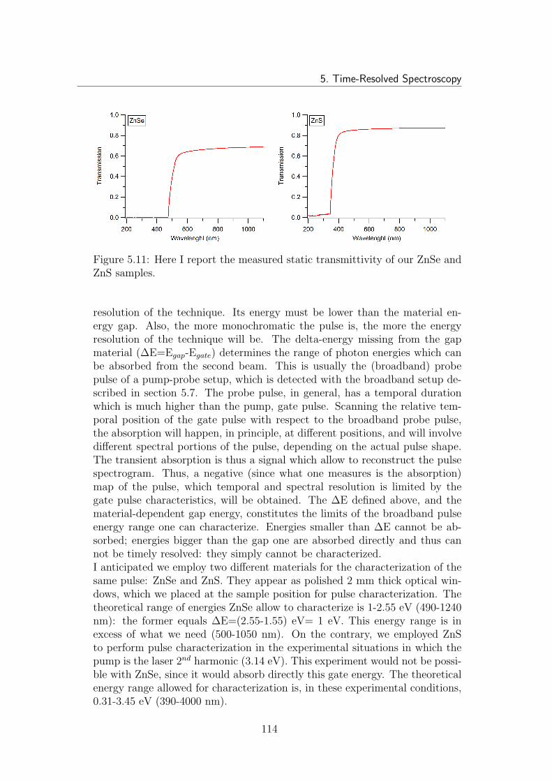
5. Time-Resolved Spectroscopy
Figure 5.11: Here I report the measured static transmittivity of our ZnSe andZnS samples.
resolution of the technique. Its energy must be lower than the material en-ergy gap. Also, the more monochromatic the pulse is, the more the energyresolution of the technique will be. The delta-energy missing from the gapmaterial (∆E=Egap-Egate) determines the range of photon energies which canbe absorbed from the second beam. This is usually the (broadband) probepulse of a pump-probe setup, which is detected with the broadband setup de-scribed in section 5.7. The probe pulse, in general, has a temporal durationwhich is much higher than the pump, gate pulse. Scanning the relative tem-poral position of the gate pulse with respect to the broadband probe pulse,the absorption will happen, in principle, at different positions, and will involvedifferent spectral portions of the pulse, depending on the actual pulse shape.The transient absorption is thus a signal which allow to reconstruct the pulsespectrogram. Thus, a negative (since what one measures is the absorption)map of the pulse, which temporal and spectral resolution is limited by thegate pulse characteristics, will be obtained. The ∆E defined above, and thematerial-dependent gap energy, constitutes the limits of the broadband pulseenergy range one can characterize. Energies smaller than ∆E cannot be ab-sorbed; energies bigger than the gap one are absorbed directly and thus cannot be timely resolved: they simply cannot be characterized.I anticipated we employ two different materials for the characterization of thesame pulse: ZnSe and ZnS. They appear as polished 2 mm thick optical win-dows, which we placed at the sample position for pulse characterization. Thetheoretical range of energies ZnSe allow to characterize is 1-2.55 eV (490-1240nm): the former equals ∆E=(2.55-1.55) eV= 1 eV. This energy range is inexcess of what we need (500-1050 nm). On the contrary, we employed ZnSto perform pulse characterization in the experimental situations in which thepump is the laser 2nd harmonic (3.14 eV). This experiment would not be possi-ble with ZnSe, since it would absorb directly this gate energy. The theoreticalenergy range allowed for characterization is, in these experimental conditions,0.31-3.45 eV (390-4000 nm).
114
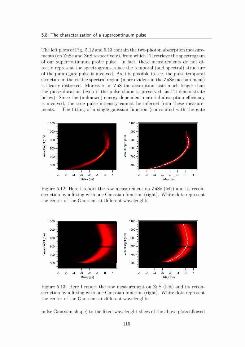
5.8. The characterization of a supercontinuum pulse
The left plots of Fig. 5.12 and 5.13 contain the two-photon absorption measure-ments (on ZnSe and ZnS respectively), from which I’ll retrieve the spectrogramof our supercontinuum probe pulse. In fact, these measurements do not di-rectly represent the spectrograms, since the temporal (and spectral) structureof the pump gate pulse is involved. As it is possible to see, the pulse temporalstructure in the visible spectral region (more evident in the ZnSe measurement)is clearly distorted. Moreover, in ZnS the absorption lasts much longer thanthe pulse duration (even if the pulse shape is preserved, as I’ll demonstratebelow). Since the (unknown) energy-dependent material absorption efficiencyis involved, the true pulse intensity cannot be inferred from these measure-ments. The fitting of a single-gaussian function (convoluted with the gate
Figure 5.12: Here I report the raw measurement on ZnSe (left) and its recon-struction by a fitting with one Gaussian function (right). White dots representthe center of the Gaussian at different wavelenghts.
Figure 5.13: Here I report the raw measurement on ZnS (left) and its recon-struction by a fitting with one Gaussian function (right). White dots representthe center of the Gaussian at different wavelenghts.
pulse Gaussian shape) to the fixed-wavelenght-slices of the above plots allowed
115
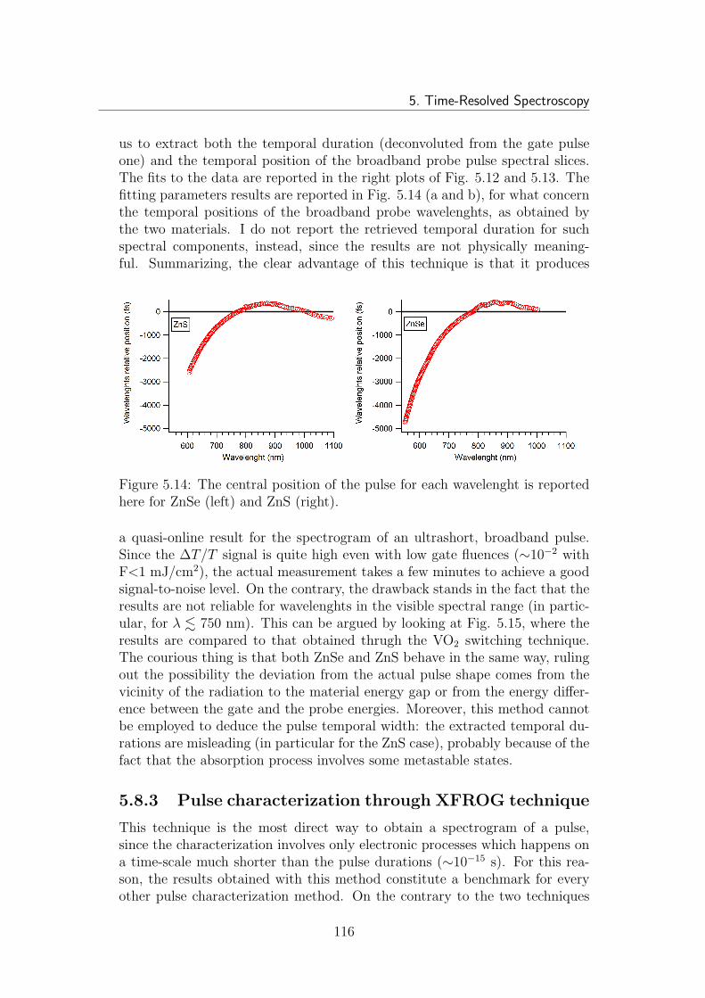
5. Time-Resolved Spectroscopy
us to extract both the temporal duration (deconvoluted from the gate pulseone) and the temporal position of the broadband probe pulse spectral slices.The fits to the data are reported in the right plots of Fig. 5.12 and 5.13. Thefitting parameters results are reported in Fig. 5.14 (a and b), for what concernthe temporal positions of the broadband probe wavelenghts, as obtained bythe two materials. I do not report the retrieved temporal duration for suchspectral components, instead, since the results are not physically meaning-ful. Summarizing, the clear advantage of this technique is that it produces
Figure 5.14: The central position of the pulse for each wavelenght is reportedhere for ZnSe (left) and ZnS (right).
a quasi-online result for the spectrogram of an ultrashort, broadband pulse.Since the ∆T/T signal is quite high even with low gate fluences (∼10−2 withF<1 mJ/cm2), the actual measurement takes a few minutes to achieve a goodsignal-to-noise level. On the contrary, the drawback stands in the fact that theresults are not reliable for wavelenghts in the visible spectral range (in partic-ular, for λ . 750 nm). This can be argued by looking at Fig. 5.15, where theresults are compared to that obtained thrugh the VO2 switching technique.The courious thing is that both ZnSe and ZnS behave in the same way, rulingout the possibility the deviation from the actual pulse shape comes from thevicinity of the radiation to the material energy gap or from the energy differ-ence between the gate and the probe energies. Moreover, this method cannotbe employed to deduce the pulse temporal width: the extracted temporal du-rations are misleading (in particular for the ZnS case), probably because of thefact that the absorption process involves some metastable states.
5.8.3 Pulse characterization through XFROG technique
This technique is the most direct way to obtain a spectrogram of a pulse,since the characterization involves only electronic processes which happens ona time-scale much shorter than the pulse durations (∼10−15 s). For this rea-son, the results obtained with this method constitute a benchmark for everyother pulse characterization method. On the contrary to the two techniques
116
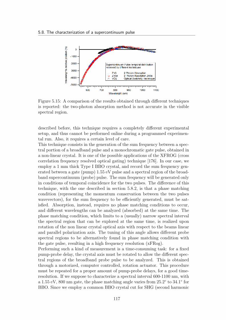
5.8. The characterization of a supercontinuum pulse
Figure 5.15: A comparison of the results obtained through different techniquesis reported: the two-photon absorption method is not accurate in the visiblespectral region.
described before, this technique requires a completely different experimentalsetup, and thus cannot be performed online during a programmed experimen-tal run. Also, it requires a certain level of care.This technique consists in the generation of the sum frequency between a spec-tral portion of a broadband pulse and a monochromatic gate pulse, obtained ina non-linear crystal. It is one of the possible applications of the XFROG (crosscorrelation frequency resolved optical gating) technique [176]. In our case, weemploy a 1 mm thick Type I BBO crystal, and record the sum frequency gen-erated between a gate (pump) 1.55 eV pulse and a spectral region of the broad-band supercontinuum (probe) pulse. The sum frequency will be generated onlyin conditions of temporal coincidence for the two pulses. The difference of thistechnique, with the one described in section 5.8.2, is that a phase matchingcondition (representing the momentum conservation between the two pulseswavevectors), for the sum frequency to be efficiently generated, must be sat-isfied. Absorption, instead, requires no phase matching conditions to occur,and different wavelengths can be analyzed (absorbed) at the same time. Thephase matching condition, which limits to a (usually) narrow spectral intervalthe spectral region that can be explored at the same time, is realized uponrotation of the non linear crystal optical axis with respect to the beams linearand parallel polarization axis. The tuning of this angle allows different probespectral regions to be alternatively found in phase matching condition withthe gate pulse, resulting in a high frequency resolution (xFRog).Performing such a kind of measurement is a time-consuming task: for a fixedpump-probe delay, the crystal axis must be rotated to allow the different spec-tral regions of the broadband probe pulse to be analyzed. This is obtainedthrough a motorized, computer controlled, rotation actuator. This proceduremust be repeated for a proper amount of pump-probe delays, for a good time-resolution. If we suppose to characterize a spectral interval 600-1100 nm, witha 1.55 eV, 800 nm gate, the phase matching angle varies from 25.2 to 34.1 forBBO. Since we employ a common BBO crystal cut for SHG (second harmonic
117
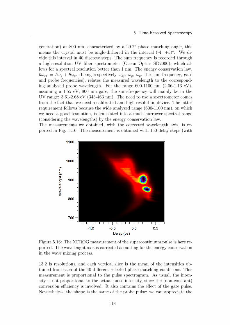
5. Time-Resolved Spectroscopy
generation) at 800 nm, characterized by a 29.2 phase matching angle, thismeans the crystal must be angle-dithered in the interval (-4, +5). We di-vide this interval in 40 discrete steps. The sum frequency is recorded througha high-resolution UV fiber spectrometer (Ocean Optics SD2000), which al-lows for a spectral resolution better than 1 nm. The energy conservation law,~ωsf = ~ωg + ~ωpr (being respectively ωsf , ωg, ωpr the sum-frequency, gateand probe frequencies), relates the measured wavelength to the correspond-ing analyzed probe wavelength. For the range 600-1100 nm (2.06-1.13 eV),assuming a 1.55 eV, 800 nm gate, the sum-frequency will mainly be in theUV range: 3.61-2.68 eV (343-463 nm). The need to use a spectrometer comesfrom the fact that we need a calibrated and high resolution device. The latterrequirement follows because the wide analyzed range (600-1100 nm), on whichwe need a good resolution, is translated into a much narrower spectral range(considering the wavelengths) by the energy conservation law.The measurements we obtained, with the corrected wavelength axis, is re-ported in Fig. 5.16. The measurement is obtained with 150 delay steps (with
Figure 5.16: The XFROG measurement of the supercontinuum pulse is here re-ported. The wavelenght axis is corrected acounting for the energy conservationin the wave mixing process.
13.2 fs resolution), and each vertical slice is the mean of the intensities ob-tained from each of the 40 different selected phase matching conditions. Thismeasurement is proportional to the pulse spectrogram. As usual, the inten-sity is not proportional to the actual pulse intensity, since the (non-constant)conversion efficiency is involved. It also contains the effect of the gate pulse.Nevertheless, the shape is the same of the probe pulse: we can appreciate the
118
5.9. Cryostat System
high spectral and temporal resolution of this technique, when compared to theprevious ones. The higher resolution allows to reveal the fine structure of thepulse, evidencing the solitonic features for ~ω < ~ωseed, being ~ωseed=1.55 eVthe PCF seed energy. The pulse extends temporally for about 1 ps in thespectral range 700-1100 nm. The pulse duration, after deconvolving for the120 fs gate pulse, is about 100 fs around 700 nm, while it increases up to ∼300fs around 1000 nm, due to the presence of solitonic structures.The clear advantage of this technique is its unbeatable resolution, both inthe spectral (thanks to the phase matching condition) and temporal (onlyelectronic processes are involved) domains. On the contrary, it requires a longtime to be performed (more than one hour, since the phase matching conditionmust be continuously tuned), and cannot be performed within the conventionalpump-supercontinuum probe setup.
5.9 Cryostat System
We employed an open cycle cryostat (Helitran LT-3-B) to allow the tempera-ture of the samples be varied in the range 10-350 K. This range can be achievedonly when the coolant is liquid helium. Also liquid nitrogen can be used ascoolant; in this case, the temperature range is limited to the interval 77-350K. The coolant is transferred from the storing dewar to the cryostat with atransfer arm. The temperature near to the sample region is accurately mea-sured with a calibrated Cernox sensor. A computer controlled heater, with aPID feedback system, stabilizes the sample temperature within ±0.1 K fromthe set temperature. The system is kept in UHV thanks to a pumping systemcomposed of a Scroll pump plus a Turbomolecular pump. A base pressure aslow as 5·10−9 mbar can be reached inside the UHV chamber; this ensures thatno sample degradation takes place, even after many hours of measurements atvery low temperatures. The UHV chamber is equipped with a CaF2 UHV op-tical window, through which the pump and probe beams reach the sample. Acopper shield shields the samples region from the rest of the chamber, limitingthe heat transfer toward the cold finger area.
119
5. Time-Resolved Spectroscopy
120
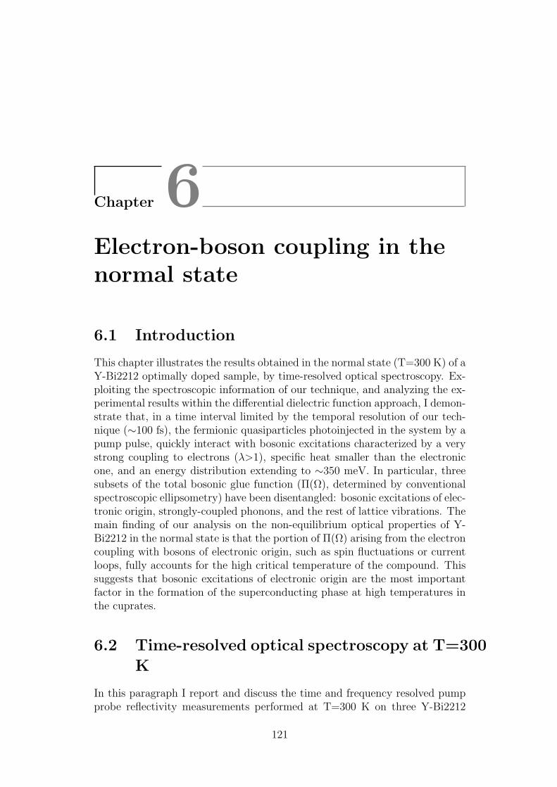
Chapter 6Electron-boson coupling in thenormal state
6.1 Introduction
This chapter illustrates the results obtained in the normal state (T=300 K) of aY-Bi2212 optimally doped sample, by time-resolved optical spectroscopy. Ex-ploiting the spectroscopic information of our technique, and analyzing the ex-perimental results within the differential dielectric function approach, I demon-strate that, in a time interval limited by the temporal resolution of our tech-nique (∼100 fs), the fermionic quasiparticles photoinjected in the system by apump pulse, quickly interact with bosonic excitations characterized by a verystrong coupling to electrons (λ>1), specific heat smaller than the electronicone, and an energy distribution extending to ∼350 meV. In particular, threesubsets of the total bosonic glue function (Π(Ω), determined by conventionalspectroscopic ellipsometry) have been disentangled: bosonic excitations of elec-tronic origin, strongly-coupled phonons, and the rest of lattice vibrations. Themain finding of our analysis on the non-equilibrium optical properties of Y-Bi2212 in the normal state is that the portion of Π(Ω) arising from the electroncoupling with bosons of electronic origin, such as spin fluctuations or currentloops, fully accounts for the high critical temperature of the compound. Thissuggests that bosonic excitations of electronic origin are the most importantfactor in the formation of the superconducting phase at high temperatures inthe cuprates.
6.2 Time-resolved optical spectroscopy at T=300
K
In this paragraph I report and discuss the time and frequency resolved pumpprobe reflectivity measurements performed at T=300 K on three Y-Bi2212
121
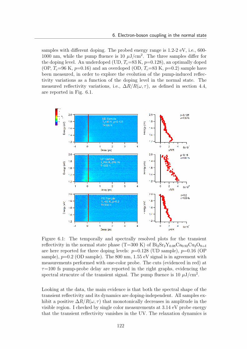
6. Electron-boson coupling in the normal state
samples with different doping. The probed energy range is 1.2-2 eV, i.e., 600-1000 nm, while the pump fluence is 10 µJ/cm2. The three samples differ forthe doping level. An underdoped (UD, Tc=83 K, p=0.128), an optimally doped(OP, Tc=96 K, p=0.16) and an overdoped (OD, Tc=83 K, p=0.2) sample havebeen measured, in order to explore the evolution of the pump-induced reflec-tivity variations as a function of the doping level in the normal state. Themeasured reflectivity variations, i.e., ∆R/R(ω, τ), as defined in section 4.4,are reported in Fig. 6.1.
Figure 6.1: The temporally and spectrally resolved plots for the transientreflectivity in the normal state phase (T=300 K) of Bi2Sr2Y0.08Ca0.92Cu2O8+δ
are here reported for three doping levels: p=0.128 (UD sample), p=0.16 (OPsample), p=0.2 (OD sample). The 800 nm, 1.55 eV signal is in agreement withmeasurements performed with one-color probe. The cuts (evidenced in red) atτ=100 fs pump-probe delay are reported in the right graphs, evidencing thespectral strucutre of the transient signal. The pump fluence is 10 µJ/cm2.
Looking at the data, the main evidence is that both the spectral shape of thetransient reflectivity and its dynamics are doping-independent. All samples ex-hibit a positive ∆R/R(ω, τ) that monotonically decreases in amplitude in thevisible region. I checked by single color measurements at 3.14 eV probe energythat the transient reflectivity vanishes in the UV. The relaxation dynamics is
122
6.2. Time-resolved optical spectroscopy at T=300 K
governed by a double exponential decay, with a fast component of about 300fs, followed by a slower one, with a decay time of about 2 ps. This doublerelaxation dynamics is usually interpreted [145, 27] as the thermalization ofthe photoinjected fermionic quasiparticles with a subset of strongly-coupledphonons (sub-ps dynamics) and the rest of the lattice (ps dynamics). Theenergy-resolved information, in this case, brings the evidence of a structurelessspectral response.
To address the microscopic origin of the measured ∆R/R(ω, τ) signal, I ex-tended the probed spectral region to the infrared, exploiting the tunable in-frared probe setup described in section 5.6. I used both the signal and idlerbeams, to cover the spectral range 0.5-1 eV (1200-2400 nm) and add dis-crete time-traces (one every 50 nm) to our time-and-energy resolved reflec-tivity plots. Here I present the obtained results only for the OP sample, onwhich the complete differential analysis will be carried on. Similar results areobtained on the underdoped and overdoped samples. The extended transientspectrum for the OP sample is presented in Fig. 6.2.
Figure 6.2: a) The measurement on the Optimally Doped sample is extendedtoward the infrared, up to 0.5 eV. b) The total transient spectra for selectedpump-probe delays τ are reported.
Thanks to the extended probed energy range (0.5-2 eV), I observe that thespectral response has a more structured form. It turns from positive in thevisible to negative in the infrared, with the crossing point which falls closeto the dressed plasma frequency of the system (∼1 eV, see Figure 3.6). On
123
6. Electron-boson coupling in the normal state
the contrary, the dynamics in the infrared is characterized by the same decayrate observed in the visible. In the infrared, the maximum reflectivity vari-ation maintains a value of about −2·10−4 up the lowest probed energy (0.5 eV).
All the analysis described in the following sections will be carried on on theoptimally-doped sample (see Fig. 6.2), since in this system the total Π(Ω) ismaximum [179], while the use of the extended Drude formalism (see Chapter3, section 5.2) still appears a reliable approximation [179, 170]. The physicalscenario disclosed by the data will be at first qualitatively described in sec-tion 6.3, while a more rigorous and quantitative approach will be adopted insections 6.4 and 6.5.
6.3 Ultrafast thermalization with bosonic ex-
citations
The aim of this section is to demonstrate that the transient spectrum shownin the left panel of Fig. 6.2 can be reproduced by a quasi-thermal scenario,within the differential dielectric function model described in section 4.4. Quasi-thermal scenario means that the measured pump-induced effect on the opticalproperties can be accounted for simply by modifying the effective temperaturesof the bosonic excitations in the Extended Drude. No other parameter in thenon-equilibrium model must be modified to reproduce the data.
The key point to extend the Extended Drude model, extensively discussedin Chapter 3, to non-equilibrium experiments is that the electron self-energy,Σ(ω, T ), entering in the calculation of ǫ(ω, τ), can be factorized into [105]:
Σ (ω, T ) =
∫ ∞
0
Π(Ω)L (ω,Ω, T ) dΩ
where L (ω,Ω, T ) is the kernel function, already defined in section 3.5.2, thataccounts for the thermal activation of the bosonic excitations and of theQPs. The kernel function L (ω,Ω, Te,b)= -2πi[N (Ω, Tb) +1/2]+Ψ(1/2+i(Ω-Ω′)/2πTe)-Ψ(1/2-i(Ω+Ω′)/2πTe), where Ψ is the Digamma function andN(Ω, Tb)the Bose distribution at temperature Tb, can be decomposed into differentterms depending on the electronic (Te) and bosonic (Tb) temperatures. Theindependent variation of Te and Tb is expected to induce different modificationsof the dielectric function.
Fig. 6.3 shows the expected relative variation of the reflectivity, i.e., ∆R/R (ω)=[R (ω, T +∆T )-R (ω, T )]/R (ω, T ), in the non-thermal (∆Te>0, ∆Tb=0) andquasi-thermal (∆Te = ∆Tb>0) scenarios. The difference between the two casesis more significant in the spectral region close to the dressed plasma frequency,Ωp≃1 eV, i.e., an energy scale much higher than the energy scale of the bosonic
124
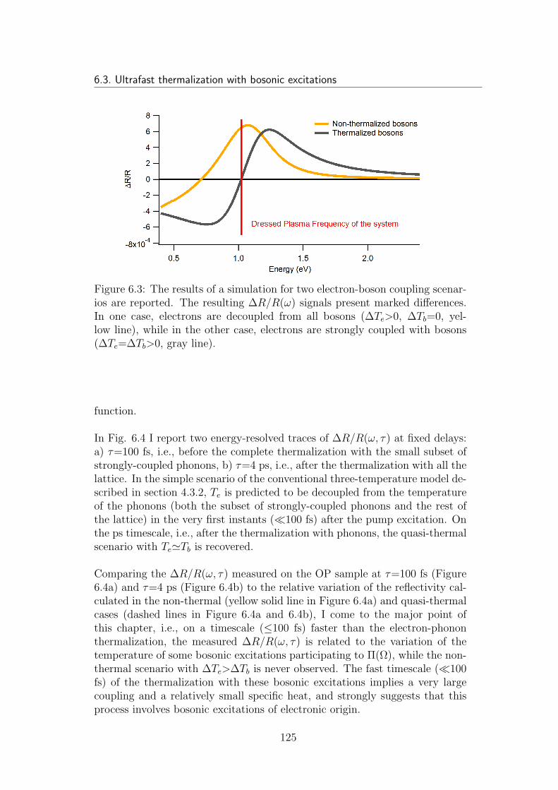
6.3. Ultrafast thermalization with bosonic excitations
Figure 6.3: The results of a simulation for two electron-boson coupling scenar-ios are reported. The resulting ∆R/R(ω) signals present marked differences.In one case, electrons are decoupled from all bosons (∆Te>0, ∆Tb=0, yel-low line), while in the other case, electrons are strongly coupled with bosons(∆Te=∆Tb>0, gray line).
function.
In Fig. 6.4 I report two energy-resolved traces of ∆R/R(ω, τ) at fixed delays:a) τ=100 fs, i.e., before the complete thermalization with the small subset ofstrongly-coupled phonons, b) τ=4 ps, i.e., after the thermalization with all thelattice. In the simple scenario of the conventional three-temperature model de-scribed in section 4.3.2, Te is predicted to be decoupled from the temperatureof the phonons (both the subset of strongly-coupled phonons and the rest ofthe lattice) in the very first instants (≪100 fs) after the pump excitation. Onthe ps timescale, i.e., after the thermalization with phonons, the quasi-thermalscenario with Te≃Tb is recovered.
Comparing the ∆R/R(ω, τ) measured on the OP sample at τ=100 fs (Figure6.4a) and τ=4 ps (Figure 6.4b) to the relative variation of the reflectivity cal-culated in the non-thermal (yellow solid line in Figure 6.4a) and quasi-thermalcases (dashed lines in Figure 6.4a and 6.4b), I come to the major point ofthis chapter, i.e., on a timescale (≤100 fs) faster than the electron-phononthermalization, the measured ∆R/R(ω, τ) is related to the variation of thetemperature of some bosonic excitations participating to Π(Ω), while the non-thermal scenario with ∆Te>∆Tb is never observed. The fast timescale (≪100fs) of the thermalization with these bosonic excitations implies a very largecoupling and a relatively small specific heat, and strongly suggests that thisprocess involves bosonic excitations of electronic origin.
125
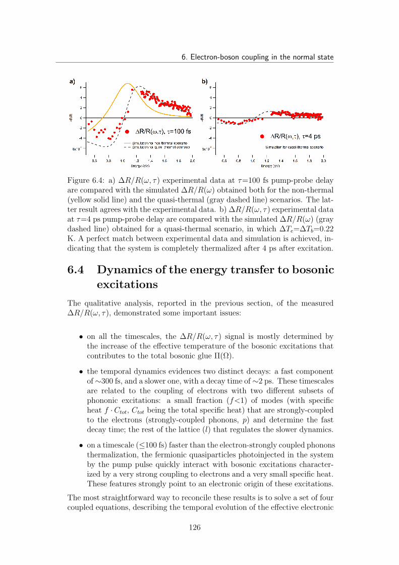
6. Electron-boson coupling in the normal state
Figure 6.4: a) ∆R/R(ω, τ) experimental data at τ=100 fs pump-probe delayare compared with the simulated ∆R/R(ω) obtained both for the non-thermal(yellow solid line) and the quasi-thermal (gray dashed line) scenarios. The lat-ter result agrees with the experimental data. b) ∆R/R(ω, τ) experimental dataat τ=4 ps pump-probe delay are compared with the simulated ∆R/R(ω) (graydashed line) obtained for a quasi-thermal scenario, in which ∆Te=∆Tb=0.22K. A perfect match between experimental data and simulation is achieved, in-dicating that the system is completely thermalized after 4 ps after excitation.
6.4 Dynamics of the energy transfer to bosonic
excitations
The qualitative analysis, reported in the previous section, of the measured∆R/R(ω, τ), demonstrated some important issues:
• on all the timescales, the ∆R/R(ω, τ) signal is mostly determined bythe increase of the effective temperature of the bosonic excitations thatcontributes to the total bosonic glue Π(Ω).
• the temporal dynamics evidences two distinct decays: a fast componentof∼300 fs, and a slower one, with a decay time of∼2 ps. These timescalesare related to the coupling of electrons with two different subsets ofphononic excitations: a small fraction (f<1) of modes (with specificheat f ·Ctot, Ctot being the total specific heat) that are strongly-coupledto the electrons (strongly-coupled phonons, p) and determine the fastdecay time; the rest of the lattice (l) that regulates the slower dynamics.
• on a timescale (≤100 fs) faster than the electron-strongly coupled phononsthermalization, the fermionic quasiparticles photoinjected in the systemby the pump pulse quickly interact with bosonic excitations character-ized by a very strong coupling to electrons and a very small specific heat.These features strongly point to an electronic origin of these excitations.
The most straightforward way to reconcile these results is to solve a set of fourcoupled equations, describing the temporal evolution of the effective electronic
126
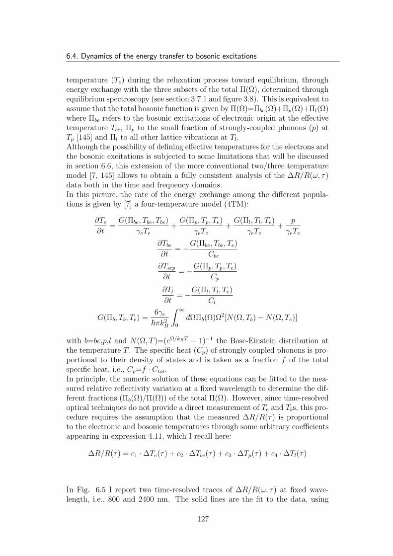
6.4. Dynamics of the energy transfer to bosonic excitations
temperature (Te) during the relaxation process toward equilibrium, throughenergy exchange with the three subsets of the total Π(Ω), determined throughequilibrium spectroscopy (see section 3.7.1 and figure 3.8). This is equivalent toassume that the total bosonic function is given by Π(Ω)=Πbe(Ω)+Πp(Ω)+Πl(Ω)where Πbe refers to the bosonic excitations of electronic origin at the effectivetemperature Tbe, Πp to the small fraction of strongly-coupled phonons (p) atTp [145] and Πl to all other lattice vibrations at Tl.Although the possibility of defining effective temperatures for the electrons andthe bosonic excitations is subjected to some limitations that will be discussedin section 6.6, this extension of the more conventional two/three temperaturemodel [7, 145] allows to obtain a fully consistent analysis of the ∆R/R(ω, τ)data both in the time and frequency domains.In this picture, the rate of the energy exchange among the different popula-tions is given by [7] a four-temperature model (4TM):
∂Te
∂t=
G(Πbe, Tbe, Tbe)
γeTe
+G(Πp, Tp, Te)
γeTe
+G(Πl, Tl, Te)
γeTe
+p
γeTe
∂Tbe
∂t= −G(Πbe, Tbe, Te)
Cbe
∂Tscp
∂t= −G(Πp, Tp, Te)
Cp
∂Tl
∂t= −G(Πl, Tl, Te)
Cl
G(Πb, Tb, Te) =6γe~πk2
B
∫ ∞
0
dΩΠb(Ω)Ω2[N(Ω, Tb)−N(Ω, Te)]
with b=be,p,l and N(Ω, T )=(eΩ/kBT − 1)−1 the Bose-Einstein distribution atthe temperature T . The specific heat (Cp) of strongly coupled phonons is pro-portional to their density of states and is taken as a fraction f of the totalspecific heat, i.e., Cp=f · Ctot.In principle, the numeric solution of these equations can be fitted to the mea-sured relative reflectivity variation at a fixed wavelength to determine the dif-ferent fractions (Πb(Ω)/Π(Ω)) of the total Π(Ω). However, since time-resolvedoptical techniques do not provide a direct measurement of Te and Tbs, this pro-cedure requires the assumption that the measured ∆R/R(τ) is proportionalto the electronic and bosonic temperatures through some arbitrary coefficientsappearing in expression 4.11, which I recall here:
∆R/R(τ) = c1 ·∆Te(τ) + c2 ·∆Tbe(τ) + c3 ·∆Tp(τ) + c4 ·∆Tl(τ)
In Fig. 6.5 I report two time-resolved traces of ∆R/R(ω, τ) at fixed wave-length, i.e., 800 and 2400 nm. The solid lines are the fit to the data, using
127
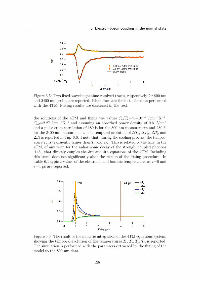
6. Electron-boson coupling in the normal state
Figure 6.5: Two fixed-wavelenght time-resolved traces, respectively for 800 nmand 2400 nm probe, are reported. Black lines are the fit to the data performedwith the 4TM. Fitting results are discussed in the text.
the solutions of the 4TM and fixing the values Ce/Te=γe=10−4 Jcm−3K−2,Ctot=2.27 Jcm−3K−1 and assuming an absorbed power density of 0.6 J/cm3
and a pulse cross-correlation of 180 fs for the 800 nm measurement and 280 fsfor the 2400 nm measurement. The temporal evolution of ∆Te, ∆Tbe, ∆Tp and∆Tl is reported in Fig. 6.6. I note that, during the cooling process, the temper-ature Tp is transiently larger than Te and Tbe. This is related to the lack, in the4TM, of any term for the anharmonic decay of the strongly coupled phonons[145], that directly couples the 3rd and 4th equations of the 4TM. Includingthis term, does not significantly alter the results of the fitting procedure. InTable 6.1 typical values of the electronic and bosonic temperatures at τ=0 andτ=4 ps are reported.
Figure 6.6: The result of the numeric integration of the 4TM equations system,showing the temporal evolution of the temperatures Te, Ts, Tp, Tl, is reported.The simulation is performed with the paramters extracted by the fitting of themodel to the 800 nm data.
128
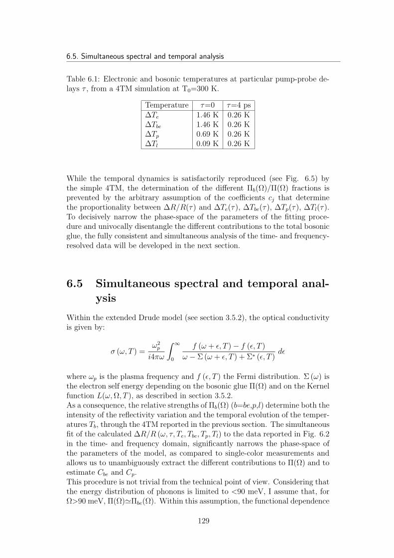
6.5. Simultaneous spectral and temporal analysis
Table 6.1: Electronic and bosonic temperatures at particular pump-probe de-lays τ , from a 4TM simulation at T0=300 K.
Temperature τ=0 τ=4 ps∆Te 1.46 K 0.26 K∆Tbe 1.46 K 0.26 K∆Tp 0.69 K 0.26 K∆Tl 0.09 K 0.26 K
While the temporal dynamics is satisfactorily reproduced (see Fig. 6.5) bythe simple 4TM, the determination of the different Πb(Ω)/Π(Ω) fractions isprevented by the arbitrary assumption of the coefficients cj that determinethe proportionality between ∆R/R(τ) and ∆Te(τ), ∆Tbe(τ), ∆Tp(τ), ∆Tl(τ).To decisively narrow the phase-space of the parameters of the fitting proce-dure and univocally disentangle the different contributions to the total bosonicglue, the fully consistent and simultaneous analysis of the time- and frequency-resolved data will be developed in the next section.
6.5 Simultaneous spectral and temporal anal-
ysis
Within the extended Drude model (see section 3.5.2), the optical conductivityis given by:
σ (ω, T ) =ω2p
i4πω
∫ ∞
0
f (ω + ǫ, T )− f (ǫ, T )
ω − Σ (ω + ǫ, T ) + Σ∗ (ǫ, T )dǫ
where ωp is the plasma frequency and f (ǫ, T ) the Fermi distribution. Σ (ω) isthe electron self energy depending on the bosonic glue Π(Ω) and on the Kernelfunction L(ω,Ω, T ), as described in section 3.5.2.As a consequence, the relative strengths of Πb(Ω) (b=be,p,l) determine both theintensity of the reflectivity variation and the temporal evolution of the temper-atures Tb, through the 4TM reported in the previous section. The simultaneousfit of the calculated ∆R/R (ω, τ, Te, Tbe, Tp, Tl) to the data reported in Fig. 6.2in the time- and frequency domain, significantly narrows the phase-space ofthe parameters of the model, as compared to single-color measurements andallows us to unambiguously extract the different contributions to Π(Ω) and toestimate Cbe and Cp.This procedure is not trivial from the technical point of view. Considering thatthe energy distribution of phonons is limited to <90 meV, I assume that, forΩ>90 meV, Π(Ω)≃Πbe(Ω). Within this assumption, the functional dependence
129
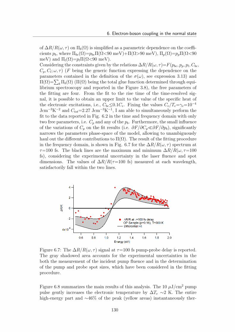
6. Electron-boson coupling in the normal state
of ∆R/R(ω, τ) on Πb(Ω) is simplified as a parametric dependence on the coeffi-cients pb, where Πbe(Ω)=pbeΠ(Ω<90 meV)+Π(Ω>90 meV), Πp(Ω)=ppΠ(Ω<90meV) and Πl(Ω)=plΠ(Ω<90 meV).Considering the constraints given by the relations ∆R/R(ω, τ)=F (pbe, pp, pl, Cbe,Cp, Cl;ω, τ) (F being the generic function expressing the dependence on theparameters contained in the definition of the σ(ω), see expression 3.13) andΠ(Ω)=
∑
b Πb(Ω) (Π(Ω) being the total glue function determined through equi-librium spectroscopy and reported in the Figure 3.8), the free parameters ofthe fitting are four. From the fit to the rise time of the time-resolved sig-nal, it is possible to obtain an upper limit to the value of the specific heat ofthe electronic excitations, i.e., Cbe≤0.1Ce. Fixing the values Ce/Te=γe=10−4
Jcm−3K−2 and Ctot=2.27 Jcm−3K−1, I am able to simultaneously perform thefit to the data reported in Fig. 6.2 in the time and frequency domain with onlytwo free parameters, i.e. Cp and any of the pb. Furthermore, the small influenceof the variations of Cp on the fit results (i.e. ∂F/∂Cp≪∂F/∂pb), significantlynarrows the parameters phase-space of the model, allowing to unambiguouslyhaul out the different contributions to Π(Ω). The result of the fitting procedurein the frequency domain, is shown in Fig. 6.7 for the ∆R/R(ω, τ) spectrum atτ=100 fs. The black lines are the maximum and minimum ∆R/R(ω, τ=100fs), considering the experimental uncertainty in the laser fluence and spotdimensions. The values of ∆R/R(τ=100 fs) measured at each wavelength,satisfactorily fall within the two lines.
Figure 6.7: The ∆R/R(ω, τ) signal at τ=100 fs pump-probe delay is reported.The gray shadowed area accounts for the experimental uncertainties in theboth the measurement of the incident pump fluence and in the determinationof the pump and probe spot sizes, which have been considered in the fittingprocedure.
Figure 6.8 summarizes the main results of this analysis. The 10 µJ/cm2 pumppulse gently increases the electronic temperature by ∆Te ∼2 K. The entirehigh-energy part and ∼46% of the peak (yellow areas) instantaneously ther-
130
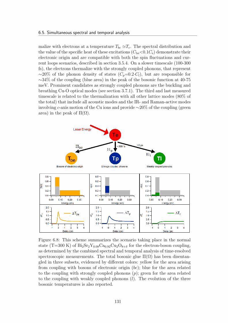
6.5. Simultaneous spectral and temporal analysis
malize with electrons at a temperature Tbe ≃Te. The spectral distribution andthe value of the specific heat of these excitations (Cbe<0.1Ce) demonstrate theirelectronic origin and are compatible with both the spin fluctuations and cur-rent loops scenarios, described in section 3.5.4. On a slower timescale (100-300fs), the electrons thermalize with the strongly coupled phonons, that represent∼20% of the phonon density of states (Cp=0.2·Cl), but are responsible for∼34% of the coupling (blue area) in the peak of the bosonic function at 40-75meV. Prominent candidates as strongly coupled phonons are the buckling andbreathing Cu-O optical modes (see section 3.7.1). The third and last measuredtimescale is related to the thermalization with all other lattice modes (80% ofthe total) that include all acoustic modes and the IR- and Raman-active modesinvolving c-axis motion of the Cu ions and provide ∼20% of the coupling (greenarea) in the peak of Π(Ω).
Figure 6.8: This scheme summarizes the scenario taking place in the normalstate (T=300 K) of Bi2Sr2Y0.08Ca0.92Cu2O8+δ for the electron-boson coupling,as determined by the combined spectral and temporal analysis of time-resolvedspectroscopic measurements. The total bosonic glue Π(Ω) has been disentan-gled in three subsets, evidenced by different colors: yellow for the area arisingfrom coupling with bosons of electronic origin (be); blue for the area relatedto the coupling with strongly coupled phonons (p); green for the area relatedto the coupling with weakly coupled phonons (l). The evolution of the threebosonic temperatures is also reported.
131
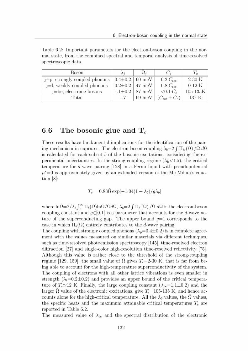
6. Electron-boson coupling in the normal state
Table 6.2: Important parameters for the electron-boson coupling in the nor-mal state, from the combined spectral and temporal analysis of time-resolvedspectroscopic data.
Boson λj Ωj Cj Tc
j=p, strongly coupled phonons 0.4±0.2 60 meV 0.2·Ctot 2-30 Kj=l, weakly coupled phonons 0.2±0.2 47 meV 0.8·Ctot 0-12 K
j=be, electronic bosons 1.1±0.2 87 meV <0.1·Ce 105-135KTotal 1.7 69 meV (Ctot + Ce) 137 K
6.6 The bosonic glue and Tc
These results have fundamental implications for the identification of the pair-ing mechanism in cuprates. The electron-boson coupling λb=2
∫
Πb (Ω) /Ω dΩis calculated for each subset b of the bosonic excitations, considering the ex-perimental uncertainties. In the strong-coupling regime (λb<1.5), the criticaltemperature for d-wave pairing [128] in a Fermi liquid with pseudopotentialµ∗=0 is approximately given by an extended version of the Mc Millan’s equa-tion [8]:
Tc = 0.83Ω exp[−1.04(1 + λb)/gλb]
where lnΩ=2/λb
∫∞
0Πb(Ω)lnΩ/ΩdΩ, λb=2
∫
Πb (Ω) /Ω dΩ is the electron-bosoncoupling constant and g∈[0,1] is a parameter that accounts for the d-wave na-ture of the superconducting gap. The upper bound g=1 corresponds to thecase in which Πb(Ω) entirely contributes to the d-wave pairing.The coupling with strongly coupled phonons (λp=0.4±0.2) is in complete agree-ment with the values measured on similar materials via different techniques,such as time-resolved photoemission spectroscopy [145], time-resolved electrondiffraction [27] and single-color high-resolution time-resolved reflectivity [75].Although this value is rather close to the threshold of the strong-couplingregime [129, 159], the small value of Ω gives Tc=2-30 K, that is far from be-ing able to account for the high-temperature superconductivity of the system.The coupling of electrons with all other lattice vibrations is even smaller instrength (λl=0.2±0.2) and provides an upper bound of the critical tempera-ture of Tc≃12 K. Finally, the large coupling constant (λbe=1.1±0.2) and thelarger Ω value of the electronic excitations, give Tc=105-135 K, and hence ac-counts alone for the high-critical temperature. All the λb values, the Ω values,the specific heats and the maximum attainable critical temperatures Tc arereported in Table 6.2.The measured value of λbe and the spectral distribution of the electronic
132
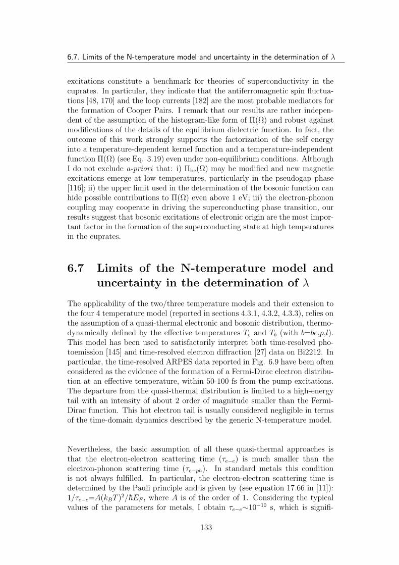
6.7. Limits of the N-temperature model and uncertainty in the determination of λ
excitations constitute a benchmark for theories of superconductivity in thecuprates. In particular, they indicate that the antiferromagnetic spin fluctua-tions [48, 170] and the loop currents [182] are the most probable mediators forthe formation of Cooper Pairs. I remark that our results are rather indepen-dent of the assumption of the histogram-like form of Π(Ω) and robust againstmodifications of the details of the equilibrium dielectric function. In fact, theoutcome of this work strongly supports the factorization of the self energyinto a temperature-dependent kernel function and a temperature-independentfunction Π(Ω) (see Eq. 3.19) even under non-equilibrium conditions. AlthoughI do not exclude a-priori that: i) Πbe(Ω) may be modified and new magneticexcitations emerge at low temperatures, particularly in the pseudogap phase[116]; ii) the upper limit used in the determination of the bosonic function canhide possible contributions to Π(Ω) even above 1 eV; iii) the electron-phononcoupling may cooperate in driving the superconducting phase transition, ourresults suggest that bosonic excitations of electronic origin are the most impor-tant factor in the formation of the superconducting state at high temperaturesin the cuprates.
6.7 Limits of the N-temperature model and
uncertainty in the determination of λ
The applicability of the two/three temperature models and their extension tothe four 4 temperature model (reported in sections 4.3.1, 4.3.2, 4.3.3), relies onthe assumption of a quasi-thermal electronic and bosonic distribution, thermo-dynamically defined by the effective temperatures Te and Tb (with b=be,p,l).This model has been used to satisfactorily interpret both time-resolved pho-toemission [145] and time-resolved electron diffraction [27] data on Bi2212. Inparticular, the time-resolved ARPES data reported in Fig. 6.9 have been oftenconsidered as the evidence of the formation of a Fermi-Dirac electron distribu-tion at an effective temperature, within 50-100 fs from the pump excitations.The departure from the quasi-thermal distribution is limited to a high-energytail with an intensity of about 2 order of magnitude smaller than the Fermi-Dirac function. This hot electron tail is usually considered negligible in termsof the time-domain dynamics described by the generic N-temperature model.
Nevertheless, the basic assumption of all these quasi-thermal approaches isthat the electron-electron scattering time (τe−e) is much smaller than theelectron-phonon scattering time (τe−ph). In standard metals this conditionis not always fulfilled. In particular, the electron-electron scattering time isdetermined by the Pauli principle and is given by (see equation 17.66 in [11]):1/τe−e=A(kBT )
2/~EF , where A is of the order of 1. Considering the typicalvalues of the parameters for metals, I obtain τe−e∼10−10 s, which is signifi-
133
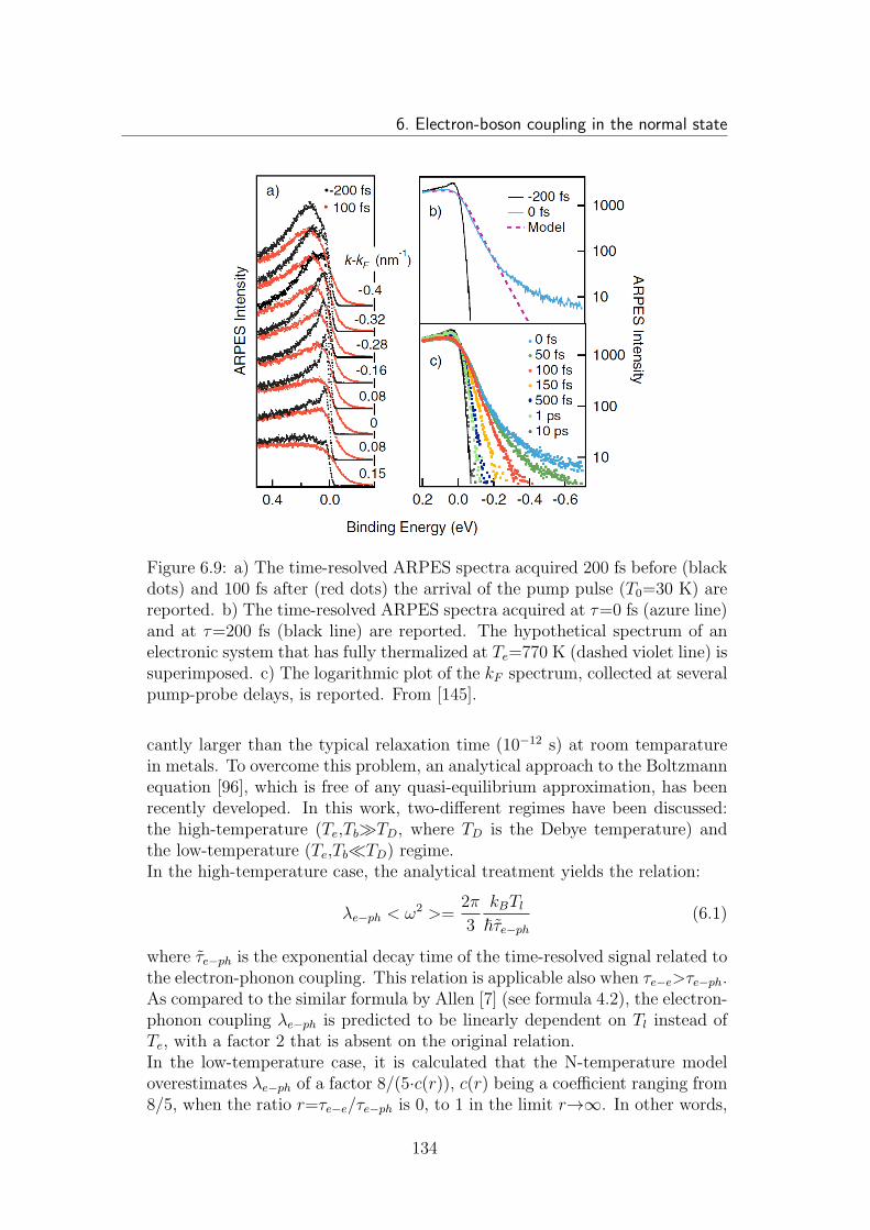
6. Electron-boson coupling in the normal state
Figure 6.9: a) The time-resolved ARPES spectra acquired 200 fs before (blackdots) and 100 fs after (red dots) the arrival of the pump pulse (T0=30 K) arereported. b) The time-resolved ARPES spectra acquired at τ=0 fs (azure line)and at τ=200 fs (black line) are reported. The hypothetical spectrum of anelectronic system that has fully thermalized at Te=770 K (dashed violet line) issuperimposed. c) The logarithmic plot of the kF spectrum, collected at severalpump-probe delays, is reported. From [145].
cantly larger than the typical relaxation time (10−12 s) at room temparaturein metals. To overcome this problem, an analytical approach to the Boltzmannequation [96], which is free of any quasi-equilibrium approximation, has beenrecently developed. In this work, two-different regimes have been discussed:the high-temperature (Te,Tb≫TD, where TD is the Debye temperature) andthe low-temperature (Te,Tb≪TD) regime.In the high-temperature case, the analytical treatment yields the relation:
λe−ph < ω2 >=2π
3
kBTl
~τe−ph
(6.1)
where τe−ph is the exponential decay time of the time-resolved signal related tothe electron-phonon coupling. This relation is applicable also when τe−e>τe−ph.As compared to the similar formula by Allen [7] (see formula 4.2), the electron-phonon coupling λe−ph is predicted to be linearly dependent on Tl instead ofTe, with a factor 2 that is absent on the original relation.In the low-temperature case, it is calculated that the N-temperature modeloverestimates λe−ph of a factor 8/(5·c(r)), c(r) being a coefficient ranging from8/5, when the ratio r=τe−e/τe−ph is 0, to 1 in the limit r→∞. In other words,
134
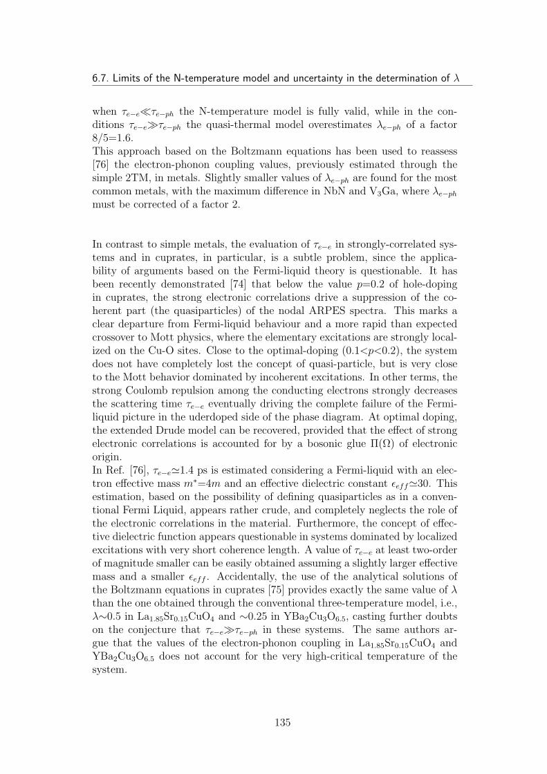
6.7. Limits of the N-temperature model and uncertainty in the determination of λ
when τe−e≪τe−ph the N-temperature model is fully valid, while in the con-ditions τe−e≫τe−ph the quasi-thermal model overestimates λe−ph of a factor8/5=1.6.This approach based on the Boltzmann equations has been used to reassess[76] the electron-phonon coupling values, previously estimated through thesimple 2TM, in metals. Slightly smaller values of λe−ph are found for the mostcommon metals, with the maximum difference in NbN and V3Ga, where λe−ph
must be corrected of a factor 2.
In contrast to simple metals, the evaluation of τe−e in strongly-correlated sys-tems and in cuprates, in particular, is a subtle problem, since the applica-bility of arguments based on the Fermi-liquid theory is questionable. It hasbeen recently demonstrated [74] that below the value p=0.2 of hole-dopingin cuprates, the strong electronic correlations drive a suppression of the co-herent part (the quasiparticles) of the nodal ARPES spectra. This marks aclear departure from Fermi-liquid behaviour and a more rapid than expectedcrossover to Mott physics, where the elementary excitations are strongly local-ized on the Cu-O sites. Close to the optimal-doping (0.1<p<0.2), the systemdoes not have completely lost the concept of quasi-particle, but is very closeto the Mott behavior dominated by incoherent excitations. In other terms, thestrong Coulomb repulsion among the conducting electrons strongly decreasesthe scattering time τe−e eventually driving the complete failure of the Fermi-liquid picture in the uderdoped side of the phase diagram. At optimal doping,the extended Drude model can be recovered, provided that the effect of strongelectronic correlations is accounted for by a bosonic glue Π(Ω) of electronicorigin.In Ref. [76], τe−e≃1.4 ps is estimated considering a Fermi-liquid with an elec-tron effective mass m∗=4m and an effective dielectric constant ǫeff≃30. Thisestimation, based on the possibility of defining quasiparticles as in a conven-tional Fermi Liquid, appears rather crude, and completely neglects the role ofthe electronic correlations in the material. Furthermore, the concept of effec-tive dielectric function appears questionable in systems dominated by localizedexcitations with very short coherence length. A value of τe−e at least two-orderof magnitude smaller can be easily obtained assuming a slightly larger effectivemass and a smaller ǫeff . Accidentally, the use of the analytical solutions ofthe Boltzmann equations in cuprates [75] provides exactly the same value of λthan the one obtained through the conventional three-temperature model, i.e.,λ∼0.5 in La1.85Sr0.15CuO4 and ∼0.25 in YBa2Cu3O6.5, casting further doubtson the conjecture that τe−e≫τe−ph in these systems. The same authors ar-gue that the values of the electron-phonon coupling in La1.85Sr0.15CuO4 andYBa2Cu3O6.5 does not account for the very high-critical temperature of thesystem.
135
6. Electron-boson coupling in the normal state
In the most pessimistic limit, i.e., τe−e≫τe−ph, the use of the solution of theBoltzmann equations to evaluate λ even strengthen the main conclusions ofthis chapter. Since in Y-Bi2212 TD∼ 300 K, our experiment falls between thelow- and high-temperature regimes discussed above. Nevertheless, I can usethe two limits to estimate the possible corrections to λp, in the case of completefailure of the N-temperature model, i.e. τe−e≫τe−ph.Adopting the expression 6.1, I obtain a value of λp< ω2 >=360-440 meV2 forthe OP sample, corresponding to λp=0.22-0.28 for a phonon frequency ω=40meV.Assuming the low-temperature limit, the maximum overestimation of λp isgiven by a factor 8/5. In our case, the fit of the 4TM to the time-resolveddata (see Figure 6.5) gives λp=0.4 that, multiplied by 5/8, gives 0.25. Thesevalues are well within the estimated range of λp=0.4±0.2, reported in section6.5. The large error bars associated to this value include: i) the experimentaluncertainty in the pump fluence; ii) the possibility of adding to the 4TM aterm that accounts for the anharmonic coupling of strongly-coupled phononsand the lattice (see section 4.3.3); iii) the possibility of the failure of the 4TMin the limit τe−e≫τe−ph. Therefore, all the conclusions about the role of thebosonic excitations of electronic origin in the formation of the superconductingcondensate are robust even against the failure of the 4TM used to reproducethe temporal dynamics of the ∆R/R(ω, τ).
I note that from the analysis of the equilibrium optical spectroscopy dataon Y-Bi2212 [178] (see Fig. 6.10), the frequency-dependent scattering timeranges from 5 fs at very low frequencies to a constant value <1 fs at about 1eV. On the basis of the results reported in this chapter, these very fast scat-tering processes are dominated by the scattering of fermionic quasiparticleswith bosonic excitations of electronic origin. Therefore, the non-equilibriumpopulation created by the pump pulse, instantaneously interacts with theseexcitations [183] before the electron-phonon scattering processes. The roleof this very fast electronic processes in quickly establishing a quasi-thermalpopulation is an open fundamental question in the field of strongly-correlatedsystems out-of-equilibrium.
I conclude this section presenting the results of the numeric integration of thesystems of equations for both the 2TM and the 4TM. The results shown inFig. 6.11 are the ∆R/R(τ) (obtained by formula 4.11 for the 4TM), normal-ized to the incident pump fluence. The electronic and the total specific heatshave the same values in both models. From the numeric solution of the systemof coupled differential equations, it is possible to argue that only in a limitof very high pump fluence the decay rate predicted by the 2TM ceases to befluence-independent. On the contrary, in the 4TM case, this effect is almostcompletely suppressed. I ascribe this result to the fact that, when the electronsare considerably heated by the absorption of an high fluence laser pulse, their
136
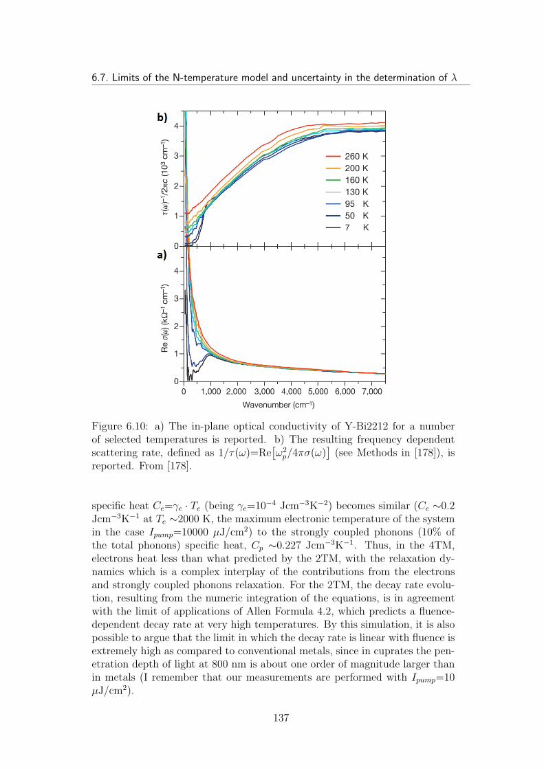
6.7. Limits of the N-temperature model and uncertainty in the determination of λ
Figure 6.10: a) The in-plane optical conductivity of Y-Bi2212 for a numberof selected temperatures is reported. b) The resulting frequency dependentscattering rate, defined as 1/τ(ω)=Re
[
ω2p/4πσ(ω)
]
(see Methods in [178]), isreported. From [178].
specific heat Ce=γe · Te (being γe=10−4 Jcm−3K−2) becomes similar (Ce ∼0.2Jcm−3K−1 at Te ∼2000 K, the maximum electronic temperature of the systemin the case Ipump=10000 µJ/cm2) to the strongly coupled phonons (10% ofthe total phonons) specific heat, Cp ∼0.227 Jcm−3K−1. Thus, in the 4TM,electrons heat less than what predicted by the 2TM, with the relaxation dy-namics which is a complex interplay of the contributions from the electronsand strongly coupled phonons relaxation. For the 2TM, the decay rate evolu-tion, resulting from the numeric integration of the equations, is in agreementwith the limit of applications of Allen Formula 4.2, which predicts a fluence-dependent decay rate at very high temperatures. By this simulation, it is alsopossible to argue that the limit in which the decay rate is linear with fluence isextremely high as compared to conventional metals, since in cuprates the pen-etration depth of light at 800 nm is about one order of magnitude larger thanin metals (I remember that our measurements are performed with Ipump=10µJ/cm2).
137
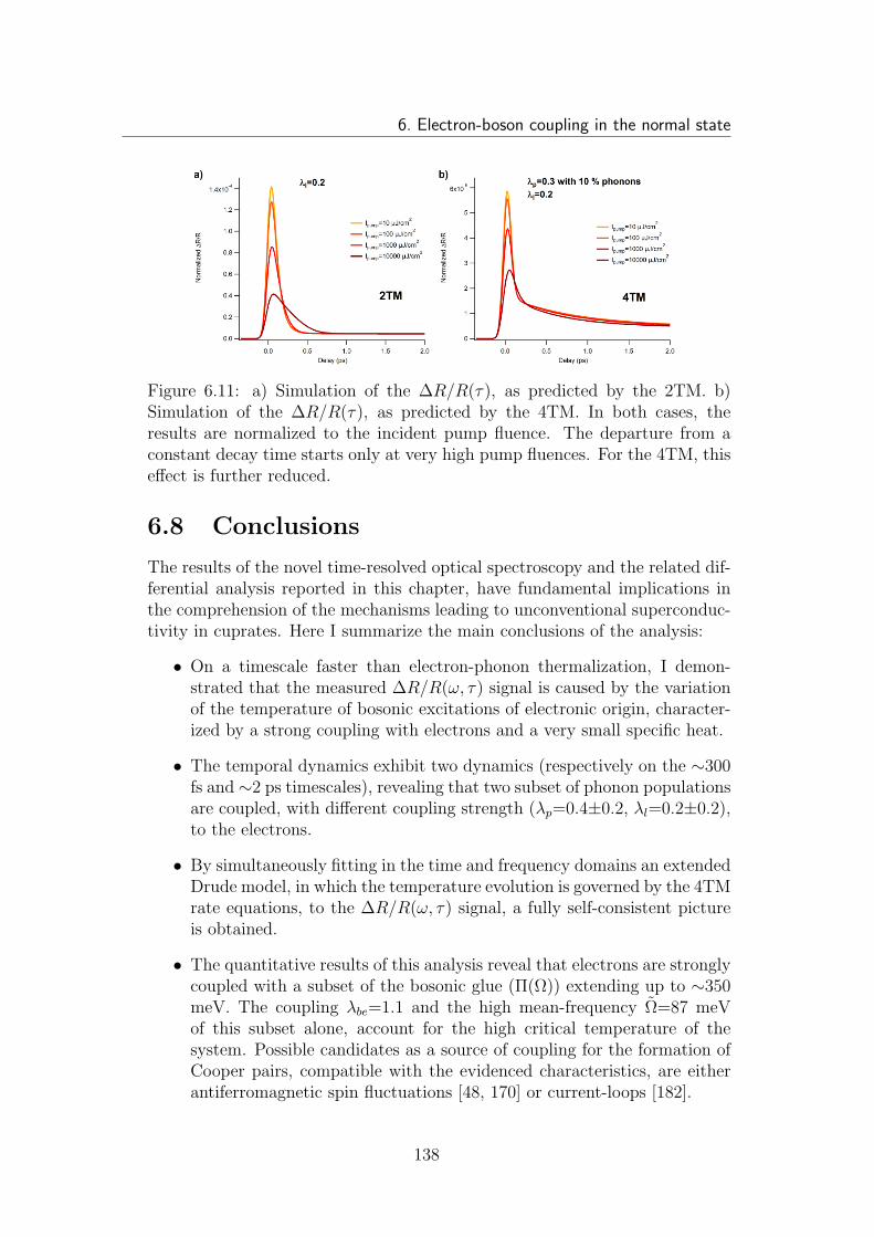
6. Electron-boson coupling in the normal state
Figure 6.11: a) Simulation of the ∆R/R(τ), as predicted by the 2TM. b)Simulation of the ∆R/R(τ), as predicted by the 4TM. In both cases, theresults are normalized to the incident pump fluence. The departure from aconstant decay time starts only at very high pump fluences. For the 4TM, thiseffect is further reduced.
6.8 Conclusions
The results of the novel time-resolved optical spectroscopy and the related dif-ferential analysis reported in this chapter, have fundamental implications inthe comprehension of the mechanisms leading to unconventional superconduc-tivity in cuprates. Here I summarize the main conclusions of the analysis:
• On a timescale faster than electron-phonon thermalization, I demon-strated that the measured ∆R/R(ω, τ) signal is caused by the variationof the temperature of bosonic excitations of electronic origin, character-ized by a strong coupling with electrons and a very small specific heat.
• The temporal dynamics exhibit two dynamics (respectively on the ∼300fs and ∼2 ps timescales), revealing that two subset of phonon populationsare coupled, with different coupling strength (λp=0.4±0.2, λl=0.2±0.2),to the electrons.
• By simultaneously fitting in the time and frequency domains an extendedDrude model, in which the temperature evolution is governed by the 4TMrate equations, to the ∆R/R(ω, τ) signal, a fully self-consistent pictureis obtained.
• The quantitative results of this analysis reveal that electrons are stronglycoupled with a subset of the bosonic glue (Π(Ω)) extending up to ∼350meV. The coupling λbe=1.1 and the high mean-frequency Ω=87 meVof this subset alone, account for the high critical temperature of thesystem. Possible candidates as a source of coupling for the formation ofCooper pairs, compatible with the evidenced characteristics, are eitherantiferromagnetic spin fluctuations [48, 170] or current-loops [182].
138
Chapter 7Excitation-dependence of thebosonic glue in the pseudogapphase
7.1 Introduction
The pseudogap state is the most exotic and elusive phase of the phase diagramof HTSCs, and the comprehension of the microscopic electronic mechanismsbehind is of paramount importance to reveal the nature of this intriguing phase.Here I demonstrate that the non-equilibrium dynamics underlying this phaseare more complex than those observed for the normal state phase, suggestingthat the pseudogap in HTSCs is a state of matter where the fermionic quasi-particles and the bosonic excitations are strongly intertwined.This chapter illustrates the results obtained by probing, with time-resolved op-tical spectroscopy, the non-equilibrium dynamics of Y-Bi2212 samples in thepseudogap phase. Measurements are performed at T=100 K, the pseudogapextending between T ∗ (∼140 K for OP samples and ∼200 K for UD samples)and Tc. In this region of the p-T phase-diagram, the transient frequency-resolved optical response is different from what observed in the normal stateand the simple quasi-thermal scenario does not account for the results.Exploiting the time- and frequency-resolution of our technique and the differ-ential analysis I demonstrate that, on the femtosecond timescale, the transientoptical response at T=100 K is dominated by an excitation-dependent bosonicglue.
139
7. Excitation-dependence of the bosonic glue in the pseudogap phase
7.2 Time-resolved spectroscopic measurements
at T=100 K
In Fig. 7.1 the time- and energy-resolved transient reflectivities ∆R/R(ω, τ)collected at T=100 K for five Y-Bi2212 samples, are reported. The samplesspan the p-T phase diagram from the underdoping to the overdoping regime,as the oxygen content δ is varied. The doping levels p of the samples are:p=0.128, p=0.16, p=0.176, p=0.197, p=0.2, corresponding to Tc values respec-tively of 83 K, 96 K, 94 K, 86 K, 83 K. In contrast to the results obtained atroom temperature (see Fig. 1 of chapter 6), when the system is in the normalstate, here the spectral response is more structured and exhibits a clear, dop-ing dependent, evolution, when moving from the underdoped to the overdopedside of the phase diagram.
The time-trace extracted from the ∆R/R(ω, τ) plot in Fig. 7.1, for the UDsample and at 1.55 eV energy, exactly reproduces the negative signal observedby conventional single-colour pump-probe measurements on underdoped sam-ples [117], at 1.55 eV probe energy. The negative time-resolved optical signalcharacterizing the non-equilibrium optical response in the visible spectral re-gion, for UD and OP samples, tends to vanish upon increasing the dopinglevel, as is evident from the right panels of Fig. 7.1. However, the ∆R/R(ω, τ)signal reveals a positive feature toward the infrared spectral region, which isalmost doping-independent and is different in intensity from the normal statesignal. The picture emerging from the ∆R/R(ω, τ) plots of Fig. 7.1 is that atT=100 K, the time resolved optical signal exhibits strongly doping-dependentspectral features. The spectroscopic information reveals mandatory for thecomprehension of the intriguing interplay of physical processes which are tak-ing place in this intriguing phase of matter. In this chapter I will demonstratethat the negative time-resolved optical signal in the visible spectral region isassociated to the onset of the pseudogap. To address the origin of the tran-sient ∆R/R(ω, τ) at T=100 K, I extended the probed spectral range to thenear infrared (0.5 eV) through an Optical Parametric Amplifier-based setup(described in section 5.6).
Fig. 7.2 reports the measurements performed on the optimally doped sample,along with some cuts of the ∆R/R(ω, τ) plot at fixed delay times, from whichthe evolution of the transient spectral response is obtained. The full transientspectrum shows two sign-change points. The first, evident from the visible-range measurements alone, is at ∼1.35 eV (i.e., ∼900 nm), whereas the secondis in the infrared part of the probed spectral range, at ∼0.6 eV (∼2050 nm),where the positive signal associated to the almost-doping-independent featurevanishes, and the impulsive reflectivity variation becomes negative on the sub-ps timescale. Although noisy, the transient signal at longer pump-probe delays(the τ=3 ps trace of Fig 7.2b can be considered) reveals an interesting feature:
140
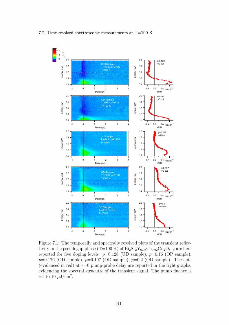
7.2. Time-resolved spectroscopic measurements at T=100 K
Figure 7.1: The temporally and spectrally resolved plots of the transient reflec-tivity in the pseudogap phase (T=100 K) of Bi2Sr2Y0.08Ca0.92Cu2O8+δ are herereported for five doping levels: p=0.128 (UD sample), p=0.16 (OP sample),p=0.176 (OD sample), p=0.197 (OD sample), p=0.2 (OD sample). The cuts(evidenced in red) at τ=0 pump-probe delay are reported in the right graphs,evidencing the spectral strucutre of the transient signal. The pump fluence isset to 10 µJ/cm2.
141
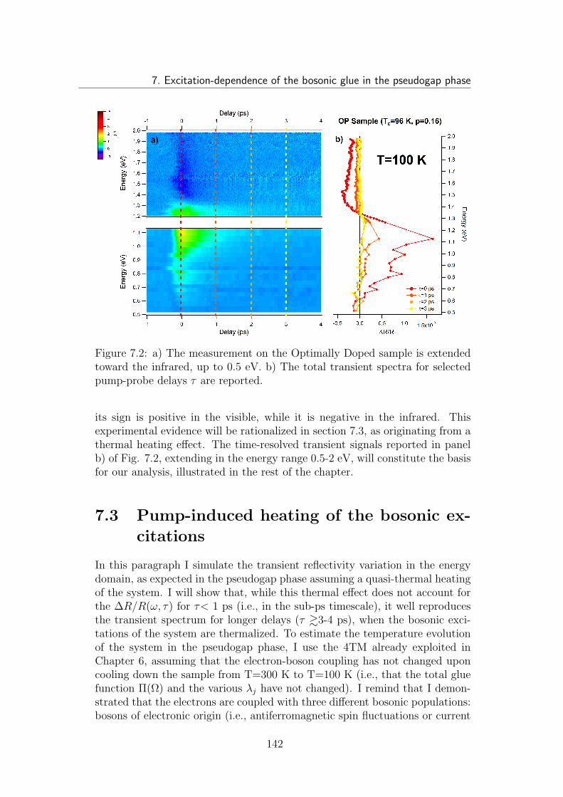
7. Excitation-dependence of the bosonic glue in the pseudogap phase
Figure 7.2: a) The measurement on the Optimally Doped sample is extendedtoward the infrared, up to 0.5 eV. b) The total transient spectra for selectedpump-probe delays τ are reported.
its sign is positive in the visible, while it is negative in the infrared. Thisexperimental evidence will be rationalized in section 7.3, as originating from athermal heating effect. The time-resolved transient signals reported in panelb) of Fig. 7.2, extending in the energy range 0.5-2 eV, will constitute the basisfor our analysis, illustrated in the rest of the chapter.
7.3 Pump-induced heating of the bosonic ex-
citations
In this paragraph I simulate the transient reflectivity variation in the energydomain, as expected in the pseudogap phase assuming a quasi-thermal heatingof the system. I will show that, while this thermal effect does not account forthe ∆R/R(ω, τ) for τ< 1 ps (i.e., in the sub-ps timescale), it well reproducesthe transient spectrum for longer delays (τ &3-4 ps), when the bosonic exci-tations of the system are thermalized. To estimate the temperature evolutionof the system in the pseudogap phase, I use the 4TM already exploited inChapter 6, assuming that the electron-boson coupling has not changed uponcooling down the sample from T=300 K to T=100 K (i.e., that the total gluefunction Π(Ω) and the various λj have not changed). I remind that I demon-strated that the electrons are coupled with three different bosonic populations:bosons of electronic origin (i.e., antiferromagnetic spin fluctuations or current
142
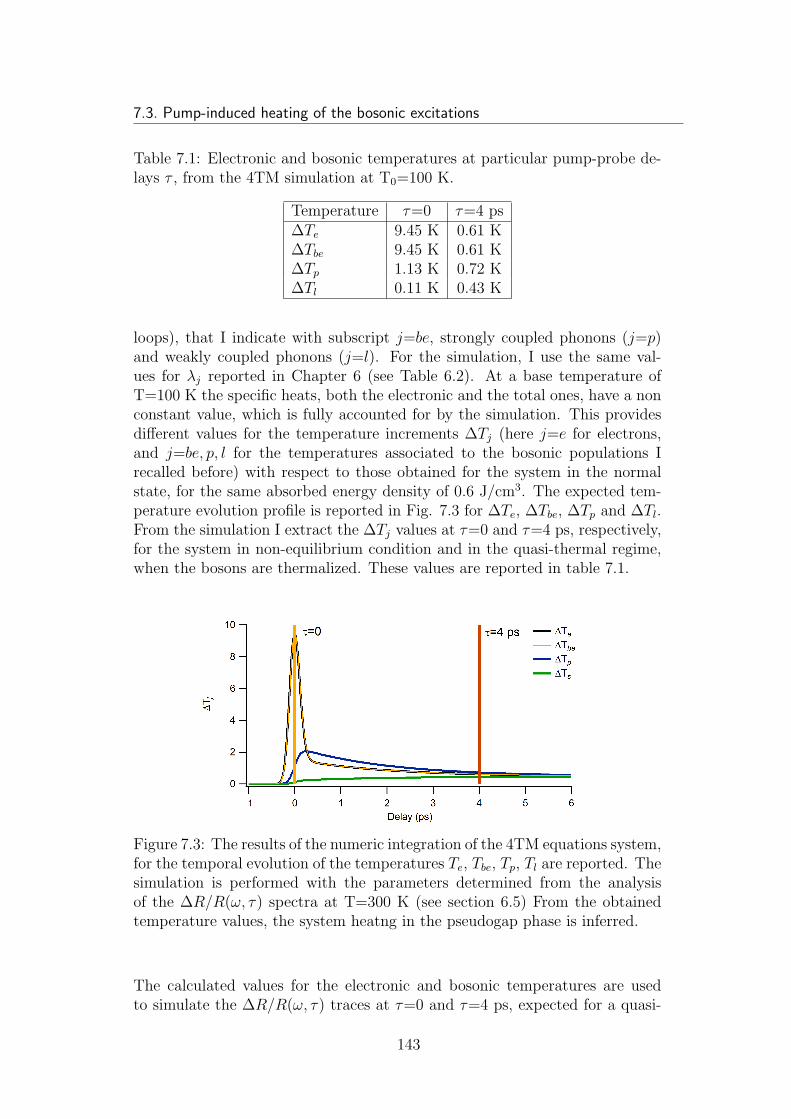
7.3. Pump-induced heating of the bosonic excitations
Table 7.1: Electronic and bosonic temperatures at particular pump-probe de-lays τ , from the 4TM simulation at T0=100 K.
Temperature τ=0 τ=4 ps∆Te 9.45 K 0.61 K∆Tbe 9.45 K 0.61 K∆Tp 1.13 K 0.72 K∆Tl 0.11 K 0.43 K
loops), that I indicate with subscript j=be, strongly coupled phonons (j=p)and weakly coupled phonons (j=l). For the simulation, I use the same val-ues for λj reported in Chapter 6 (see Table 6.2). At a base temperature ofT=100 K the specific heats, both the electronic and the total ones, have a nonconstant value, which is fully accounted for by the simulation. This providesdifferent values for the temperature increments ∆Tj (here j=e for electrons,and j=be, p, l for the temperatures associated to the bosonic populations Irecalled before) with respect to those obtained for the system in the normalstate, for the same absorbed energy density of 0.6 J/cm3. The expected tem-perature evolution profile is reported in Fig. 7.3 for ∆Te, ∆Tbe, ∆Tp and ∆Tl.From the simulation I extract the ∆Tj values at τ=0 and τ=4 ps, respectively,for the system in non-equilibrium condition and in the quasi-thermal regime,when the bosons are thermalized. These values are reported in table 7.1.
Figure 7.3: The results of the numeric integration of the 4TM equations system,for the temporal evolution of the temperatures Te, Tbe, Tp, Tl are reported. Thesimulation is performed with the parameters determined from the analysisof the ∆R/R(ω, τ) spectra at T=300 K (see section 6.5) From the obtainedtemperature values, the system heatng in the pseudogap phase is inferred.
The calculated values for the electronic and bosonic temperatures are usedto simulate the ∆R/R(ω, τ) traces at τ=0 and τ=4 ps, expected for a quasi-
143
7. Excitation-dependence of the bosonic glue in the pseudogap phase
thermal scenario. This simulation has been done with the differential dielectricfunction approach (see section 4.4) and the EDM presented in section 3.5.2.For clarity, I recall here the main expressions of this model. The Drude partof the model dielectric function, related to the reflectivity by formula 3.3, isgiven by:
ǫD(ω, T ) = 1− ωp2
ω(ω + iM(ω, T ))(7.1)
Where the Memory function M(ω, T ), given by:
M(ω, T ) = −iω
∫ +∞
−∞
f(ξ, T )− f(ξ + ω, T )
ω + Σ∗(ξ, T )− Σ(ξ + ω, T ) + iγimp
dξ
−1
+ iω (7.2)
is a function of the electronic self-energy Σ(ω, T ), which is given by (in themodel presented in 3.5.2):
Σ(ω, T ) =
∫ ∞
0
α2F (Ω)L(ω,Ω, T )dΩ (7.3)
where the Kernel function L(ω,Ω, T ) writes:
L(ω,Ω, T ) = −2πi
[
n(Ω, T ) +1
2
]
+Ψ
(
1
2+ i
Ω− Ω′
2πT
)
−Ψ
(
1
2− i
Ω + Ω′
2πT
)
(7.4)
It must be noted that in our simulations, the Glue Function Π(Ω), appearingin equation 7.3 and expressing the electron-boson coupling is held constant(i.e., independent from the heating given by the laser excitation), while onlythe temperatures appearing in the BE (n) and FD (f) distributions of theKernel function (equation 7.4), which describes the thermal excitations of theelectrons and the glue, are changed. Values from Table 7.1 are considered.The Glue Function Π(Ω) is factorized in three subsets, as illustrated in Fig.6.8. Each one has its own bosonic temperature Tb: Tbe, Tp, Tl, entering theKernel function L(ω,Ω, T ).The temporal traces obtained by the simulation described are reported in Fig.7.4 and Fig. 7.5, respectively for τ = 0 and τ = 4 ps, together with theexperimental data. Comparing the results of the simulation to the measured∆R/R(ω, τ) traces, I come to the major point of this section. That is, whilethe spectrum obtained for the system 4 ps after excitation is well reproducedby a quasi-thermal scenario, the spectrum at zero delay requires a more com-plex picture than that of a purely (non-thermal) heating effect.
Fig. 7.4 clearly shows that the experimental and the simulated spectra, for apump-probe delay of τ=0 ps, are significantly different. In particular, a nega-tive time-resolved optical signal is observed in the visible spectral region, and
144
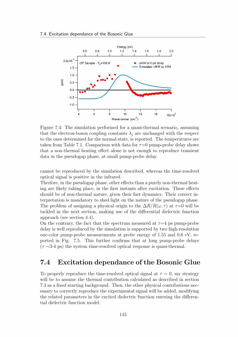
7.4. Excitation dependance of the Bosonic Glue
Figure 7.4: The simulation performed for a quasi-thermal scenario, assumingthat the electron-boson coupling constants λj are unchanged with the respectto the ones determined for the normal state, is reported. The temperatures aretaken from Table 7.1. Comparison with data for τ=0 pump-probe delay showsthat a non-thermal heating effect alone is not enough to reproduce transientdata in the pseudogap phase, at small pump-probe delay.
cannot be reproduced by the simulation described, whereas the time-resolvedoptical signal is positive in the infrared.Therfore, in the pseudogap phase, other effects than a purely non-thermal heat-ing are likely taking place, in the first instants after excitation. These effectsshould be of non-thermal nature, given their fast dynamics. Their correct in-terpretation is mandatory to shed light on the nature of the pseudogap phase.The problem of assigning a physical origin to the ∆R/R(ω, τ) at τ=0 will betackled in the next section, making use of the differential dielectric functionapproach (see section 4.4).On the contrary, the fact that the spectrum measured at τ=4 ps pump-probedelay is well reproduced by the simulation is supported by two high-resolutionone-color pump-probe measurements at probe energy of 1.55 and 0.6 eV, re-ported in Fig. 7.5. This further confirms that at long pump-probe delays(τ ∼3-4 ps) the system time-resolved optical response is quasi-thermal.
7.4 Excitation dependance of the Bosonic Glue
To properly reproduce the time-resolved optical signal at τ = 0, my strategywill be to assume the thermal contribution calculated as described in section7.3 as a fixed starting background. Then, the other physical contributions nec-essary to correctly reproduce the experimental signal will be added, modifyingthe related parameters in the excited dielectric function entering the differen-tial dielectric function model.
145
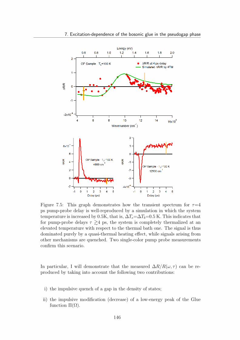
7. Excitation-dependence of the bosonic glue in the pseudogap phase
Figure 7.5: This graph demonstrates how the transient spectrum for τ=4ps pump-probe delay is well-reproduced by a simulation in which the systemtemperature is increased by 0.5K, that is, ∆Te=∆Tb=0.5 K. This indicates thatfor pump-probe delays τ &4 ps, the system is completely thermalized at anelevated temperature with respect to the thermal bath one. The signal is thusdominated purely by a quasi-thermal heating effect, while signals arising fromother mechanisms are quenched. Two single-color pump probe measurementsconfirm this scenario.
In particular, I will demonstrate that the measured ∆R/R(ω, τ) can be re-produced by taking into account the following two contributions:
i) the impulsive quench of a gap in the density of states;
ii) the impulsive modification (decrease) of a low-energy peak of the Gluefunction Π(Ω).
146
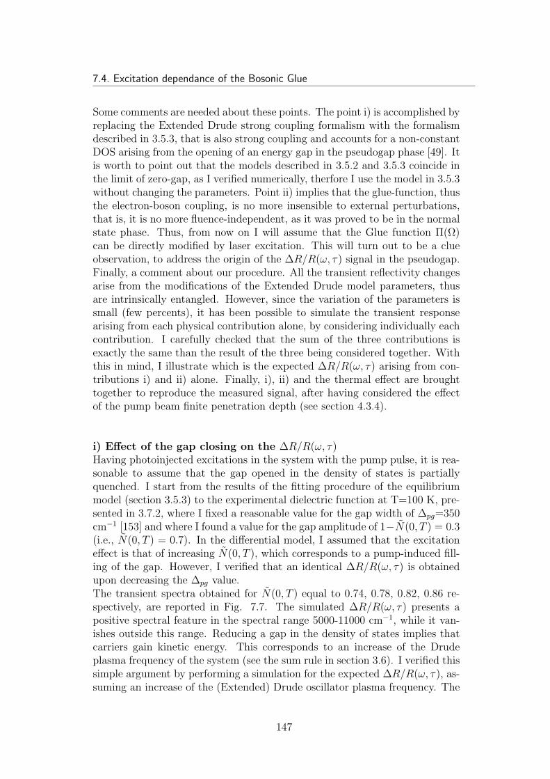
7.4. Excitation dependance of the Bosonic Glue
Some comments are needed about these points. The point i) is accomplished byreplacing the Extended Drude strong coupling formalism with the formalismdescribed in 3.5.3, that is also strong coupling and accounts for a non-constantDOS arising from the opening of an energy gap in the pseudogap phase [49]. Itis worth to point out that the models described in 3.5.2 and 3.5.3 coincide inthe limit of zero-gap, as I verified numerically, therfore I use the model in 3.5.3without changing the parameters. Point ii) implies that the glue-function, thusthe electron-boson coupling, is no more insensible to external perturbations,that is, it is no more fluence-independent, as it was proved to be in the normalstate phase. Thus, from now on I will assume that the Glue function Π(Ω)can be directly modified by laser excitation. This will turn out to be a clueobservation, to address the origin of the ∆R/R(ω, τ) signal in the pseudogap.Finally, a comment about our procedure. All the transient reflectivity changesarise from the modifications of the Extended Drude model parameters, thusare intrinsically entangled. However, since the variation of the parameters issmall (few percents), it has been possible to simulate the transient responsearising from each physical contribution alone, by considering individually eachcontribution. I carefully checked that the sum of the three contributions isexactly the same than the result of the three being considered together. Withthis in mind, I illustrate which is the expected ∆R/R(ω, τ) arising from con-tributions i) and ii) alone. Finally, i), ii) and the thermal effect are broughttogether to reproduce the measured signal, after having considered the effectof the pump beam finite penetration depth (see section 4.3.4).
i) Effect of the gap closing on the ∆R/R(ω, τ)Having photoinjected excitations in the system with the pump pulse, it is rea-sonable to assume that the gap opened in the density of states is partiallyquenched. I start from the results of the fitting procedure of the equilibriummodel (section 3.5.3) to the experimental dielectric function at T=100 K, pre-sented in 3.7.2, where I fixed a reasonable value for the gap width of ∆pg=350cm−1 [153] and where I found a value for the gap amplitude of 1−N(0, T ) = 0.3(i.e., N(0, T ) = 0.7). In the differential model, I assumed that the excitationeffect is that of increasing N(0, T ), which corresponds to a pump-induced fill-ing of the gap. However, I verified that an identical ∆R/R(ω, τ) is obtainedupon decreasing the ∆pg value.The transient spectra obtained for N(0, T ) equal to 0.74, 0.78, 0.82, 0.86 re-spectively, are reported in Fig. 7.7. The simulated ∆R/R(ω, τ) presents apositive spectral feature in the spectral range 5000-11000 cm−1, while it van-ishes outside this range. Reducing a gap in the density of states implies thatcarriers gain kinetic energy. This corresponds to an increase of the Drudeplasma frequency of the system (see the sum rule in section 3.6). I verified thissimple argument by performing a simulation for the expected ∆R/R(ω, τ), as-suming an increase of the (Extended) Drude oscillator plasma frequency. The
147
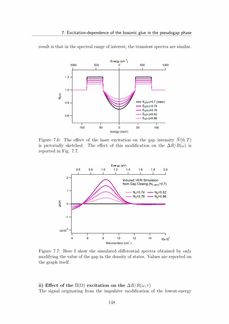
7. Excitation-dependence of the bosonic glue in the pseudogap phase
result is that in the spectral range of interest, the transient spectra are similar.
Figure 7.6: The effect of the laser excitation on the gap intensity N(0, T )is pictorially sketched. The effect of this modification on the ∆R/R(ω) isreported in Fig. 7.7.
Figure 7.7: Here I show the simulated differential spectra obtained by onlymodifying the value of the gap in the density of states. Values are reported onthe graph itself.
ii) Effect of the Π(Ω) excitation on the ∆R/R(ω, τ)The signal originating from the impulsive modification of the lowest-energy
148
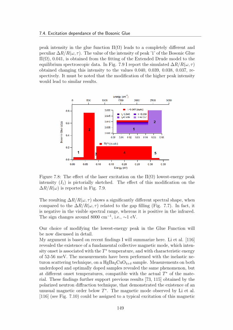
7.4. Excitation dependance of the Bosonic Glue
peak intensity in the glue function Π(Ω) leads to a completely different andpeculiar ∆R/R(ω, τ). The value of the intensity of peak ’1’ of the Bosonic GlueΠ(Ω), 0.041, is obtained from the fitting of the Extended Drude model to theequilibrium spectroscopic data. In Fig. 7.9 I report the simulated ∆R/R(ω, τ)obtained changing this intensity to the values 0.040, 0.039, 0.038, 0.037, re-spectively. It must be noted that the modification of the higher peak intensitywould lead to similar results.
Figure 7.8: The effect of the laser excitation on the Π(Ω) lowest-energy peakintensity (I1) is pictorially sketched. The effect of this modification on the∆R/R(ω) is reported in Fig. 7.9.
The resulting ∆R/R(ω, τ) shows a significantly different spectral shape, whencompared to the ∆R/R(ω, τ) related to the gap filling (Fig. 7.7). In fact, itis negative in the visible spectral range, whereas it is positive in the infrared.The sign changes around 8000 cm−1, i.e., ∼1 eV.
Our choice of modifying the lowest-energy peak in the Glue Function willbe now discussed in detail.My argument is based on recent findings I will summarize here. Li et al. [116]revealed the existence of a fundamental collective magnetic mode, which inten-sity onset is associated with the T ∗ temperature, and with characteristic energyof 52-56 meV. The measurements have been performed with the inelastic ne-turon scattering technique, on a HgBa2CuO4+δ sample. Measurements on bothunderdoped and optimally doped samples revealed the same phenomenon, butat different onset temperatures, compatible with the actual T ∗ of the mate-rial. These findings further support previous results [73, 115] obtained by thepolarized neutron diffraction technique, that demonstrated the existence of anunusual magnetic order below T ∗. The magnetic mode observed by Li et al.[116] (see Fig. 7.10) could be assigned to a typical excitation of this magnetic
149
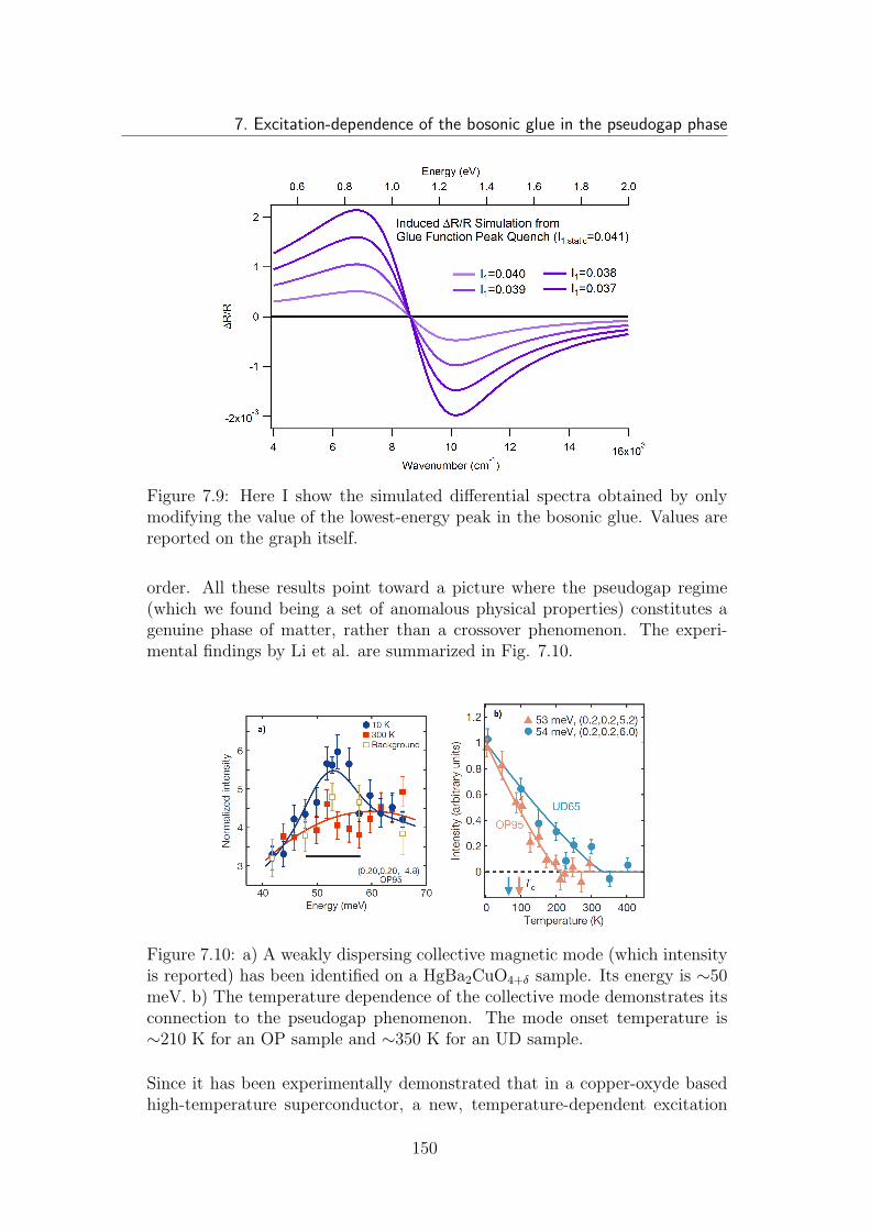
7. Excitation-dependence of the bosonic glue in the pseudogap phase
Figure 7.9: Here I show the simulated differential spectra obtained by onlymodifying the value of the lowest-energy peak in the bosonic glue. Values arereported on the graph itself.
order. All these results point toward a picture where the pseudogap regime(which we found being a set of anomalous physical properties) constitutes agenuine phase of matter, rather than a crossover phenomenon. The experi-mental findings by Li et al. are summarized in Fig. 7.10.
Figure 7.10: a) A weakly dispersing collective magnetic mode (which intensityis reported) has been identified on a HgBa2CuO4+δ sample. Its energy is ∼50meV. b) The temperature dependence of the collective mode demonstrates itsconnection to the pseudogap phenomenon. The mode onset temperature is∼210 K for an OP sample and ∼350 K for an UD sample.
Since it has been experimentally demonstrated that in a copper-oxyde basedhigh-temperature superconductor, a new, temperature-dependent excitation
150
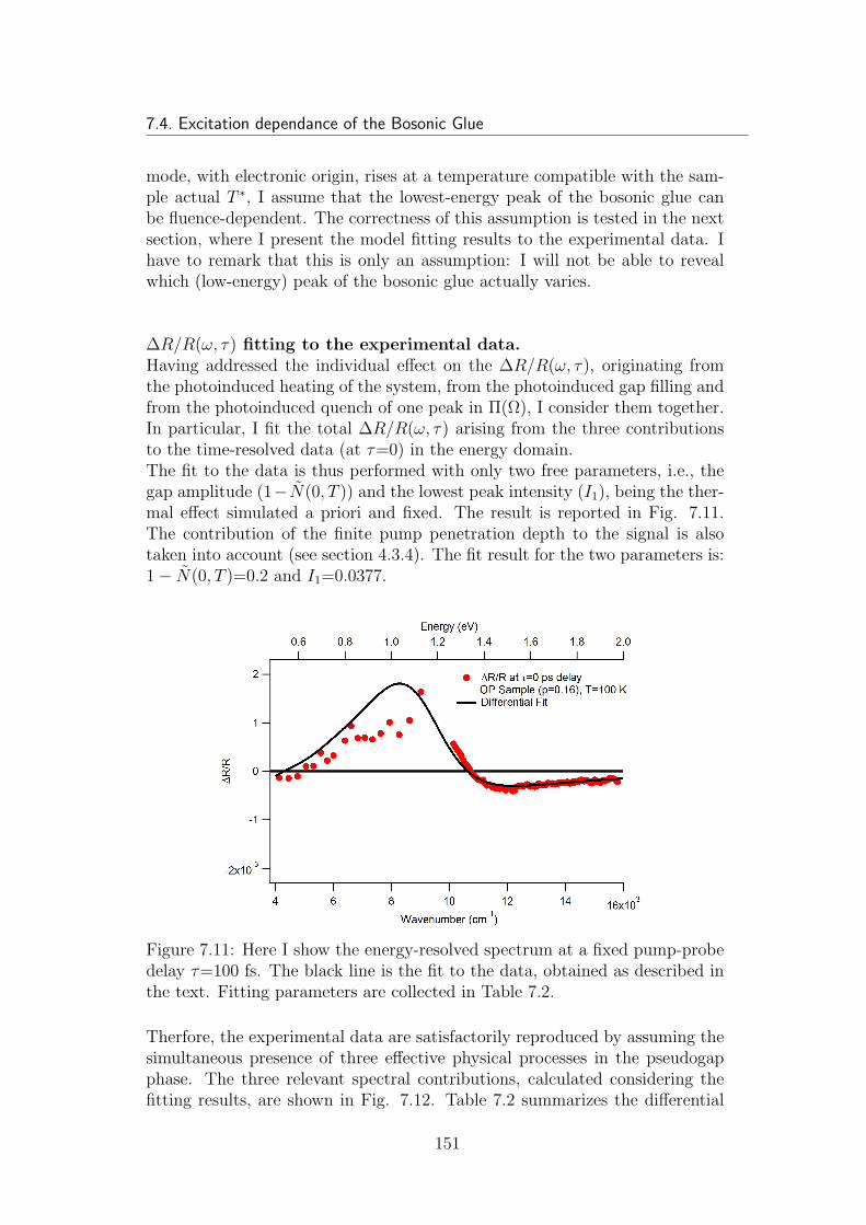
7.4. Excitation dependance of the Bosonic Glue
mode, with electronic origin, rises at a temperature compatible with the sam-ple actual T ∗, I assume that the lowest-energy peak of the bosonic glue canbe fluence-dependent. The correctness of this assumption is tested in the nextsection, where I present the model fitting results to the experimental data. Ihave to remark that this is only an assumption: I will not be able to revealwhich (low-energy) peak of the bosonic glue actually varies.
∆R/R(ω, τ) fitting to the experimental data.Having addressed the individual effect on the ∆R/R(ω, τ), originating fromthe photoinduced heating of the system, from the photoinduced gap filling andfrom the photoinduced quench of one peak in Π(Ω), I consider them together.In particular, I fit the total ∆R/R(ω, τ) arising from the three contributionsto the time-resolved data (at τ=0) in the energy domain.The fit to the data is thus performed with only two free parameters, i.e., thegap amplitude (1−N(0, T )) and the lowest peak intensity (I1), being the ther-mal effect simulated a priori and fixed. The result is reported in Fig. 7.11.The contribution of the finite pump penetration depth to the signal is alsotaken into account (see section 4.3.4). The fit result for the two parameters is:1− N(0, T )=0.2 and I1=0.0377.
Figure 7.11: Here I show the energy-resolved spectrum at a fixed pump-probedelay τ=100 fs. The black line is the fit to the data, obtained as described inthe text. Fitting parameters are collected in Table 7.2.
Therfore, the experimental data are satisfactorily reproduced by assuming thesimultaneous presence of three effective physical processes in the pseudogapphase. The three relevant spectral contributions, calculated considering thefitting results, are shown in Fig. 7.12. Table 7.2 summarizes the differential
151
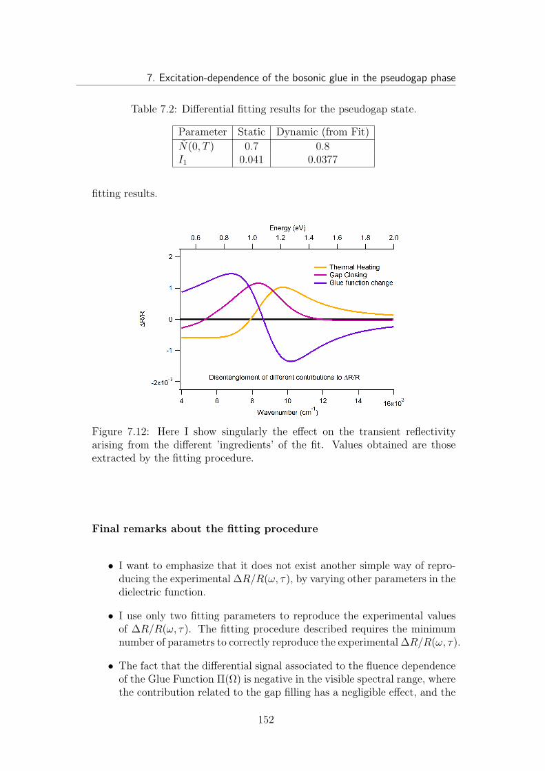
7. Excitation-dependence of the bosonic glue in the pseudogap phase
Table 7.2: Differential fitting results for the pseudogap state.
Parameter Static Dynamic (from Fit)
N(0, T ) 0.7 0.8I1 0.041 0.0377
fitting results.
Figure 7.12: Here I show singularly the effect on the transient reflectivityarising from the different ’ingredients’ of the fit. Values obtained are thoseextracted by the fitting procedure.
Final remarks about the fitting procedure
• I want to emphasize that it does not exist another simple way of repro-ducing the experimental ∆R/R(ω, τ), by varying other parameters in thedielectric function.
• I use only two fitting parameters to reproduce the experimental valuesof ∆R/R(ω, τ). The fitting procedure described requires the minimumnumber of parametrs to correctly reproduce the experimental ∆R/R(ω, τ).
• The fact that the differential signal associated to the fluence dependenceof the Glue Function Π(Ω) is negative in the visible spectral range, wherethe contribution related to the gap filling has a negligible effect, and the
152
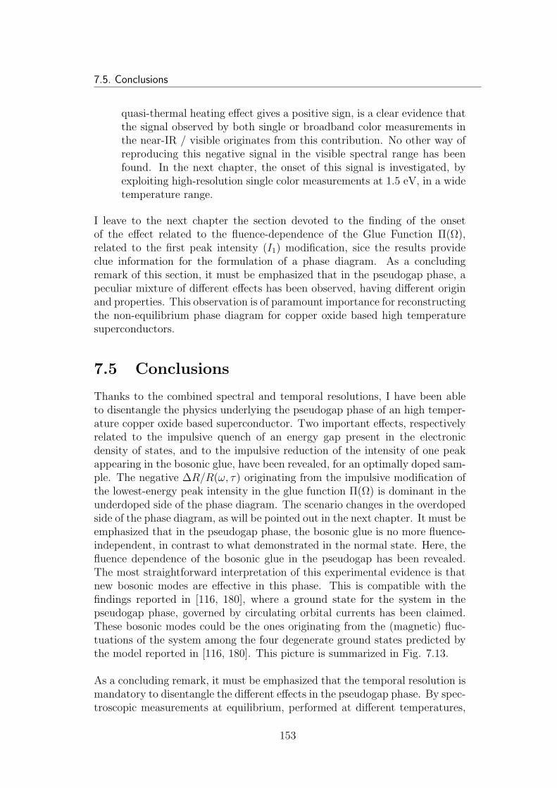
7.5. Conclusions
quasi-thermal heating effect gives a positive sign, is a clear evidence thatthe signal observed by both single or broadband color measurements inthe near-IR / visible originates from this contribution. No other way ofreproducing this negative signal in the visible spectral range has beenfound. In the next chapter, the onset of this signal is investigated, byexploiting high-resolution single color measurements at 1.5 eV, in a widetemperature range.
I leave to the next chapter the section devoted to the finding of the onsetof the effect related to the fluence-dependence of the Glue Function Π(Ω),related to the first peak intensity (I1) modification, sice the results provideclue information for the formulation of a phase diagram. As a concludingremark of this section, it must be emphasized that in the pseudogap phase, apeculiar mixture of different effects has been observed, having different originand properties. This observation is of paramount importance for reconstructingthe non-equilibrium phase diagram for copper oxide based high temperaturesuperconductors.
7.5 Conclusions
Thanks to the combined spectral and temporal resolutions, I have been ableto disentangle the physics underlying the pseudogap phase of an high temper-ature copper oxide based superconductor. Two important effects, respectivelyrelated to the impulsive quench of an energy gap present in the electronicdensity of states, and to the impulsive reduction of the intensity of one peakappearing in the bosonic glue, have been revealed, for an optimally doped sam-ple. The negative ∆R/R(ω, τ) originating from the impulsive modification ofthe lowest-energy peak intensity in the glue function Π(Ω) is dominant in theunderdoped side of the phase diagram. The scenario changes in the overdopedside of the phase diagram, as will be pointed out in the next chapter. It must beemphasized that in the pseudogap phase, the bosonic glue is no more fluence-independent, in contrast to what demonstrated in the normal state. Here, thefluence dependence of the bosonic glue in the pseudogap has been revealed.The most straightforward interpretation of this experimental evidence is thatnew bosonic modes are effective in this phase. This is compatible with thefindings reported in [116, 180], where a ground state for the system in thepseudogap phase, governed by circulating orbital currents has been claimed.These bosonic modes could be the ones originating from the (magnetic) fluc-tuations of the system among the four degenerate ground states predicted bythe model reported in [116, 180]. This picture is summarized in Fig. 7.13.
As a concluding remark, it must be emphasized that the temporal resolution ismandatory to disentangle the different effects in the pseudogap phase. By spec-troscopic measurements at equilibrium, performed at different temperatures,
153
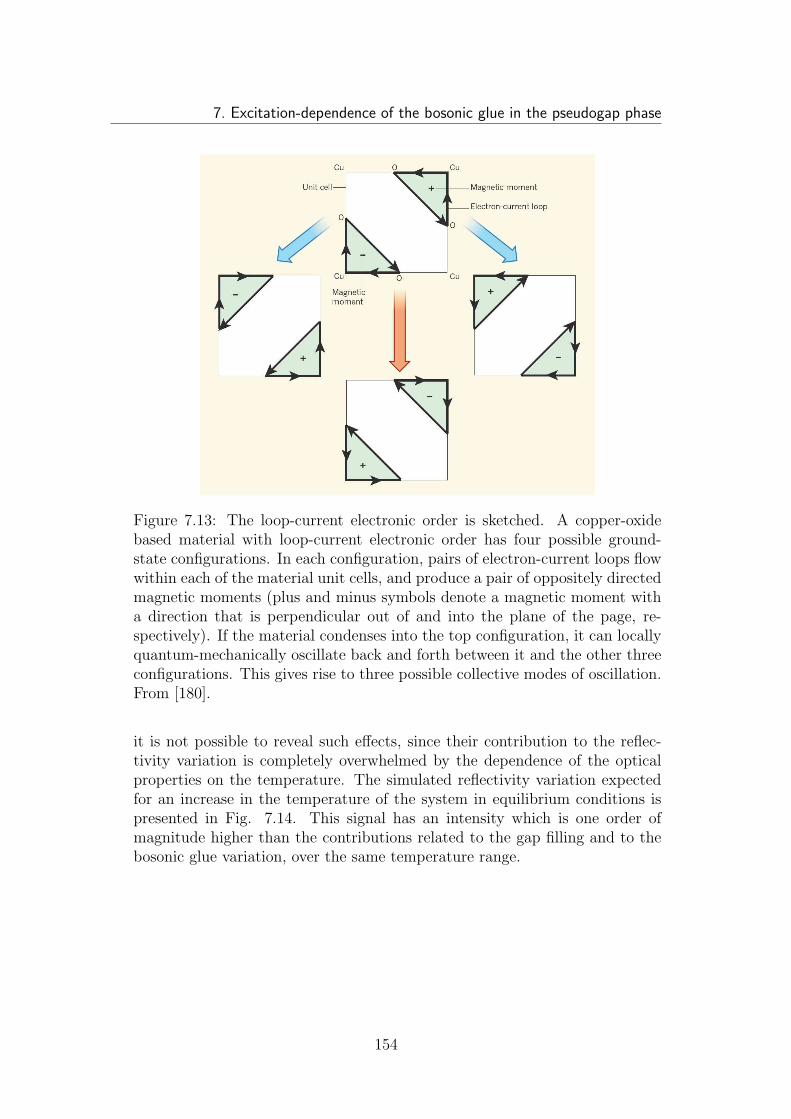
7. Excitation-dependence of the bosonic glue in the pseudogap phase
Figure 7.13: The loop-current electronic order is sketched. A copper-oxidebased material with loop-current electronic order has four possible ground-state configurations. In each configuration, pairs of electron-current loops flowwithin each of the material unit cells, and produce a pair of oppositely directedmagnetic moments (plus and minus symbols denote a magnetic moment witha direction that is perpendicular out of and into the plane of the page, re-spectively). If the material condenses into the top configuration, it can locallyquantum-mechanically oscillate back and forth between it and the other threeconfigurations. This gives rise to three possible collective modes of oscillation.From [180].
it is not possible to reveal such effects, since their contribution to the reflec-tivity variation is completely overwhelmed by the dependence of the opticalproperties on the temperature. The simulated reflectivity variation expectedfor an increase in the temperature of the system in equilibrium conditions ispresented in Fig. 7.14. This signal has an intensity which is one order ofmagnitude higher than the contributions related to the gap filling and to thebosonic glue variation, over the same temperature range.
154
7.5. Conclusions
Figure 7.14: In the left plot, I calculate the difference in reflectivity obtainedby heating the system, from T0=100 K, to 150, 200, 250, 300 K. In the rightplot, the ∆R/R arising from the same effect is calculated. In the inset, thestatic reflectivity for T0=100 K is shown.
155
7. Excitation-dependence of the bosonic glue in the pseudogap phase
156
Chapter 8The Phase Diagram fromNon-Equilibrium Spectroscopy
8.1 Introduction
The aim of this final chapter is to summarize all the results of the novel time-resolved spectroscopy developed and used in this work. The response to anultrashort excitation of the normal, pseudogap and superconducting phases ofthe copper-oxide high-temperature superconductor Bi2Sr2Ca0.92Y0.08Cu2O8+δ,provides a new comprehensive picture of the phase diagram of this system.The chapter will start with the description of the non-equilibrium propertiesof the system in the superconducting state, that have not been presented yet.In contrast to what observed in the normal state and pseudogap phases, in thesuperconducting phase the transient optical response in the near-IR / visiblespectral range can only be interpreted by assuming a pump-induced modifi-cation of the high-energy dielectric function. I demonstrate that two opticalinterband transitions at 1.5 and 2 eV are intimately related to the conden-sate formation at Tc. The long-standing debate about the interplay betweenhigh- and low-energy physics in these compounds, as a function of doping, isfinally addressed. In the superconducting state, the optical response is stronglydoping-dependent, with a clear crossover close to the optimal doping level re-quired to attain the maximum critical temperature Tc for the BSCCO family.This crossover delimits two regions in which superconductivity is driven byan opposite mechanism: on the underdoped side of the phase diagram, super-conductivity is driven by a direct kinetic energy gain (lowering), while on theoverdoped side of the phase diagram, superconductivity is accompanied by aBCS-line kinetic energy loss, overcompensated by a gain in potential energy.In this context, the superconductivity-induced variation of the spectral weightof the interband transitions at 1.5 and 2 eV, fully accunts for the kynetic en-ergy variation over the whole phase diagram.This observation will be extremely helpful to the construction of a non-equilibrium
157
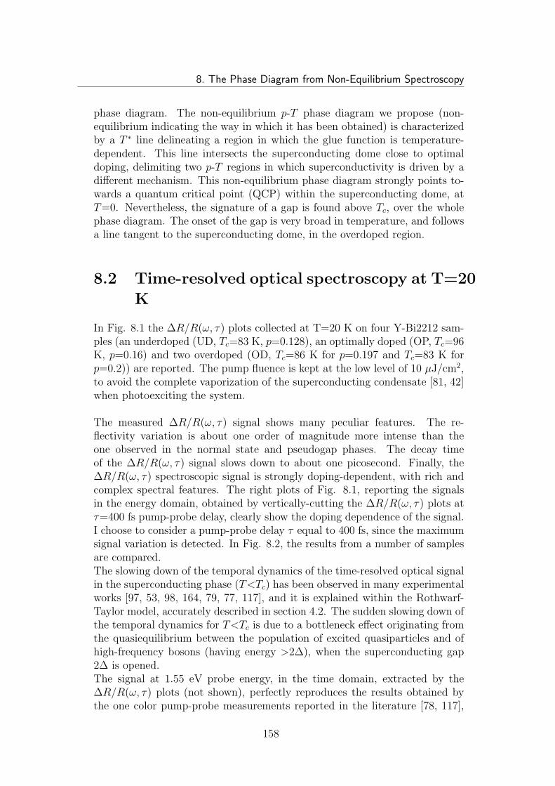
8. The Phase Diagram from Non-Equilibrium Spectroscopy
phase diagram. The non-equilibrium p-T phase diagram we propose (non-equilibrium indicating the way in which it has been obtained) is characterizedby a T ∗ line delineating a region in which the glue function is temperature-dependent. This line intersects the superconducting dome close to optimaldoping, delimiting two p-T regions in which superconductivity is driven by adifferent mechanism. This non-equilibrium phase diagram strongly points to-wards a quantum critical point (QCP) within the superconducting dome, atT=0. Nevertheless, the signature of a gap is found above Tc, over the wholephase diagram. The onset of the gap is very broad in temperature, and followsa line tangent to the superconducting dome, in the overdoped region.
8.2 Time-resolved optical spectroscopy at T=20
K
In Fig. 8.1 the ∆R/R(ω, τ) plots collected at T=20 K on four Y-Bi2212 sam-ples (an underdoped (UD, Tc=83 K, p=0.128), an optimally doped (OP, Tc=96K, p=0.16) and two overdoped (OD, Tc=86 K for p=0.197 and Tc=83 K forp=0.2)) are reported. The pump fluence is kept at the low level of 10 µJ/cm2,to avoid the complete vaporization of the superconducting condensate [81, 42]when photoexciting the system.
The measured ∆R/R(ω, τ) signal shows many peculiar features. The re-flectivity variation is about one order of magnitude more intense than theone observed in the normal state and pseudogap phases. The decay timeof the ∆R/R(ω, τ) signal slows down to about one picosecond. Finally, the∆R/R(ω, τ) spectroscopic signal is strongly doping-dependent, with rich andcomplex spectral features. The right plots of Fig. 8.1, reporting the signalsin the energy domain, obtained by vertically-cutting the ∆R/R(ω, τ) plots atτ=400 fs pump-probe delay, clearly show the doping dependence of the signal.I choose to consider a pump-probe delay τ equal to 400 fs, since the maximumsignal variation is detected. In Fig. 8.2, the results from a number of samplesare compared.The slowing down of the temporal dynamics of the time-resolved optical signalin the superconducting phase (T<Tc) has been observed in many experimentalworks [97, 53, 98, 164, 79, 77, 117], and it is explained within the Rothwarf-Taylor model, accurately described in section 4.2. The sudden slowing down ofthe temporal dynamics for T<Tc is due to a bottleneck effect originating fromthe quasiequilibrium between the population of excited quasiparticles and ofhigh-frequency bosons (having energy >2∆), when the superconducting gap2∆ is opened.The signal at 1.55 eV probe energy, in the time domain, extracted by the∆R/R(ω, τ) plots (not shown), perfectly reproduces the results obtained bythe one color pump-probe measurements reported in the literature [78, 117],
158
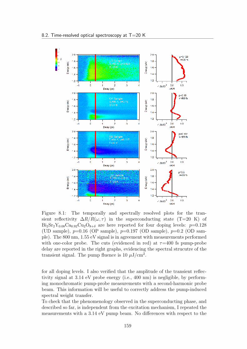
8.2. Time-resolved optical spectroscopy at T=20 K
Figure 8.1: The temporally and spectrally resolved plots for the tran-sient reflectivity ∆R/R(ω, τ) in the superconducting state (T=20 K) ofBi2Sr2Y0.08Ca0.92Cu2O8+δ are here reported for four doping levels: p=0.128(UD sample), p=0.16 (OP sample), p=0.197 (OD sample), p=0.2 (OD sam-ple). The 800 nm, 1.55 eV signal is in agreement with measurements performedwith one-color probe. The cuts (evidenced in red) at τ=400 fs pump-probedelay are reported in the right graphs, evidencing the spectral strucutre of thetransient signal. The pump fluence is 10 µJ/cm2.
for all doping levels. I also verified that the amplitude of the transient reflec-tivity signal at 3.14 eV probe energy (i.e., 400 nm) is negligible, by perform-ing monochromatic pump-probe measurements with a second-harmonic probebeam. This information will be useful to correctly address the pump-inducedspectral weight transfer.To check that the phenomenology observed in the superconducting phase, anddescribed so far, is independent from the excitation mechanism, I repeated themeasurements with a 3.14 eV pump beam. No differences with respect to the
159
8. The Phase Diagram from Non-Equilibrium Spectroscopy
measurements reported in Fig. 8.1, performed with a 1.55 eV pump beam,emerged. This ensures what we observed is related to an intrinsic response ofthe superconducting phase, independent of the excitation mechanism.In Fig. 8.2, I show the transient reflectivity spectra for a pump-probe delayequal to τ=400 fs, for a number of samples with different dopings. The tracesfor the samples with p=0.128 (UD sample), p=0.16 (OP1 sample (red dots),the same sample which reslts are presented in Fig. 8.1), and p=0.197 (ODsample) will constitute the basis for our differential analysis.
Figure 8.2: The spectrally resolved reflectivity traces at T=20 K, for a pump-probe delay equal to τ=400 fs and a pump fluence equal to 10 µJ/cm2, arereported here for a number of different samples. While OP samples OP1, OP2,OP3 have the same nominal doping (p=0.16), sample OP3 has been exposedto air for a longer time, resulting in a slight increase of the Oxygen content.
By directly comparing the ∆R/R(ω, τ) cuts at τ=400 fs pump-probe delay,the evolution of the spectroscopic signal with doping can be argued. By in-creasing the doping level, the all-positive reflectivity variation characterizingthe underdoped sample is gradually modified by a suppression of the signalaround 1.4 eV, which eventually evolves into a negative feature in the 1.1-1.5eV energy range for the overdoped sample.
8.3 Transient reflectivity in the superconduct-
ing phase
In this paragraph I present the results of the fitting of the differential di-electric function model (described in 4.4) to the ∆R/R(ω, τ) traces at fixedpump-probe delays, for the UD (p=0.128), OP1 (p=0.16) and OD (p=0.197)samples. Experimental data and the fitting results are presented in Fig. 8.3.For all doping levels, the interpretation of the structured ∆R/R(ω, τ) in the
160
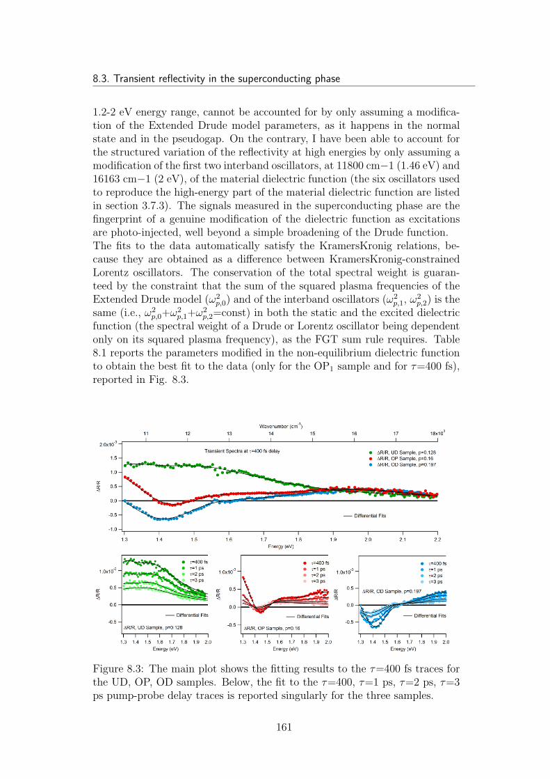
8.3. Transient reflectivity in the superconducting phase
1.2-2 eV energy range, cannot be accounted for by only assuming a modifica-tion of the Extended Drude model parameters, as it happens in the normalstate and in the pseudogap. On the contrary, I have been able to account forthe structured variation of the reflectivity at high energies by only assuming amodification of the first two interband oscillators, at 11800 cm−1 (1.46 eV) and16163 cm−1 (2 eV), of the material dielectric function (the six oscillators usedto reproduce the high-energy part of the material dielectric function are listedin section 3.7.3). The signals measured in the superconducting phase are thefingerprint of a genuine modification of the dielectric function as excitationsare photo-injected, well beyond a simple broadening of the Drude function.The fits to the data automatically satisfy the KramersKronig relations, be-cause they are obtained as a difference between KramersKronig-constrainedLorentz oscillators. The conservation of the total spectral weight is guaran-teed by the constraint that the sum of the squared plasma frequencies of theExtended Drude model (ω2
p,0) and of the interband oscillators (ω2p,1, ω
2p,2) is the
same (i.e., ω2p,0+ω2
p,1+ω2p,2=const) in both the static and the excited dielectric
function (the spectral weight of a Drude or Lorentz oscillator being dependentonly on its squared plasma frequency), as the FGT sum rule requires. Table8.1 reports the parameters modified in the non-equilibrium dielectric functionto obtain the best fit to the data (only for the OP1 sample and for τ=400 fs),reported in Fig. 8.3.
Figure 8.3: The main plot shows the fitting results to the τ=400 fs traces forthe UD, OP, OD samples. Below, the fit to the τ=400, τ=1 ps, τ=2 ps, τ=3ps pump-probe delay traces is reported singularly for the three samples.
161
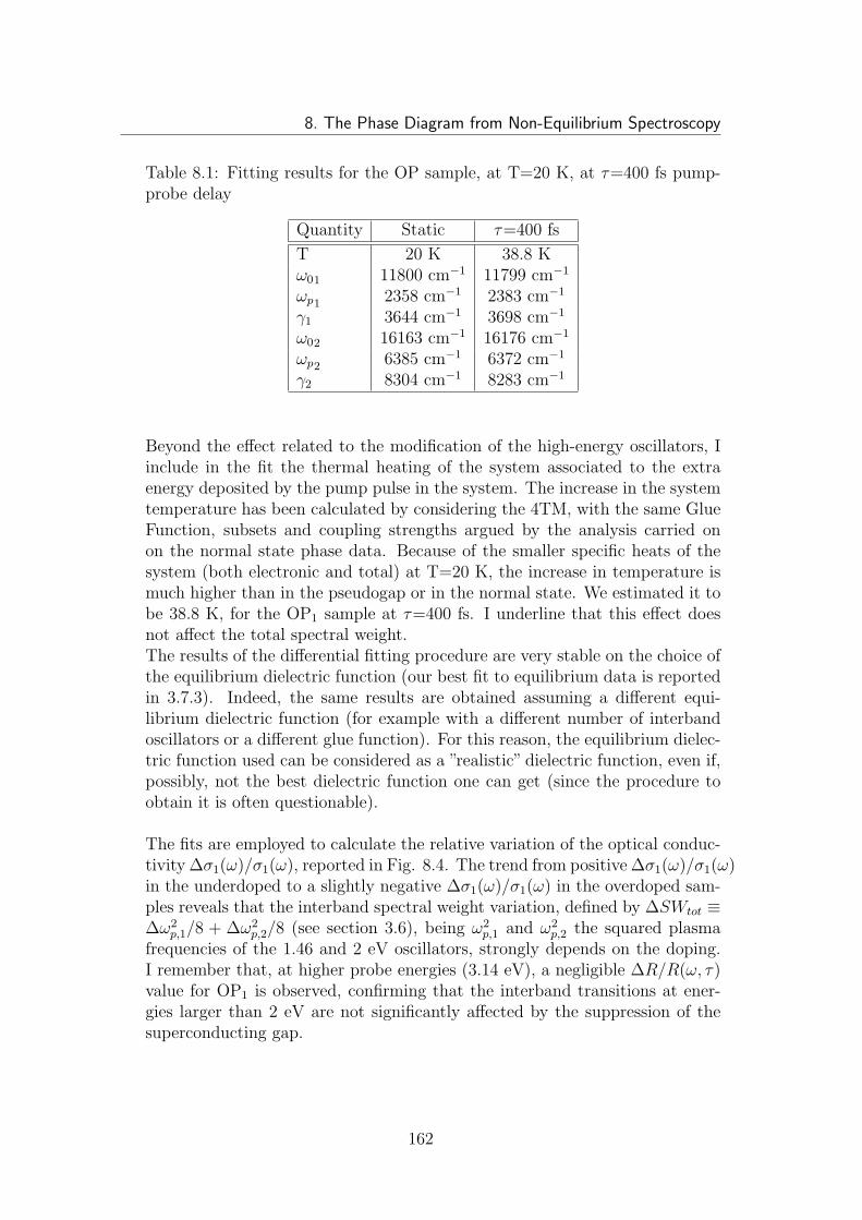
8. The Phase Diagram from Non-Equilibrium Spectroscopy
Table 8.1: Fitting results for the OP sample, at T=20 K, at τ=400 fs pump-probe delay
Quantity Static τ=400 fs
T 20 K 38.8 Kω01 11800 cm−1 11799 cm−1
ωp1 2358 cm−1 2383 cm−1
γ1 3644 cm−1 3698 cm−1
ω02 16163 cm−1 16176 cm−1
ωp2 6385 cm−1 6372 cm−1
γ2 8304 cm−1 8283 cm−1
Beyond the effect related to the modification of the high-energy oscillators, Iinclude in the fit the thermal heating of the system associated to the extraenergy deposited by the pump pulse in the system. The increase in the systemtemperature has been calculated by considering the 4TM, with the same GlueFunction, subsets and coupling strengths argued by the analysis carried onon the normal state phase data. Because of the smaller specific heats of thesystem (both electronic and total) at T=20 K, the increase in temperature ismuch higher than in the pseudogap or in the normal state. We estimated it tobe 38.8 K, for the OP1 sample at τ=400 fs. I underline that this effect doesnot affect the total spectral weight.The results of the differential fitting procedure are very stable on the choice ofthe equilibrium dielectric function (our best fit to equilibrium data is reportedin 3.7.3). Indeed, the same results are obtained assuming a different equi-librium dielectric function (for example with a different number of interbandoscillators or a different glue function). For this reason, the equilibrium dielec-tric function used can be considered as a ”realistic” dielectric function, even if,possibly, not the best dielectric function one can get (since the procedure toobtain it is often questionable).
The fits are employed to calculate the relative variation of the optical conduc-tivity ∆σ1(ω)/σ1(ω), reported in Fig. 8.4. The trend from positive ∆σ1(ω)/σ1(ω)in the underdoped to a slightly negative ∆σ1(ω)/σ1(ω) in the overdoped sam-ples reveals that the interband spectral weight variation, defined by ∆SWtot ≡∆ω2
p,1/8 + ∆ω2p,2/8 (see section 3.6), being ω2
p,1 and ω2p,2 the squared plasma
frequencies of the 1.46 and 2 eV oscillators, strongly depends on the doping.I remember that, at higher probe energies (3.14 eV), a negligible ∆R/R(ω, τ)value for OP1 is observed, confirming that the interband transitions at ener-gies larger than 2 eV are not significantly affected by the suppression of thesuperconducting gap.
162
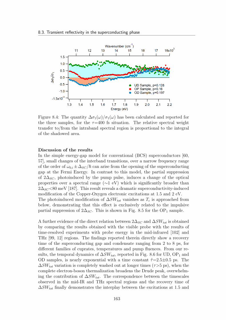
8.3. Transient reflectivity in the superconducting phase
Figure 8.4: The quantity ∆σ1(ω)/σ1(ω) has been calculated and reported forthe three samples, for the τ=400 fs situation. The relative spectral weighttransfer to/from the intraband spectral region is proportional to the integralof the shadowed area.
Discussion of the resultsIn the simple energy-gap model for conventional (BCS) superconductors [60,57], small changes of the interband transitions, over a narrow frequency rangeof the order of ω0,i±∆SC/~ can arise from the opening of the superconductinggap at the Fermi Energy. In contrast to this model, the partial suppressionof 2∆SC , photoinduced by the pump pulse, induces a change of the opticalproperties over a spectral range (∼1 eV) which is significantly broader than2∆SC<80 meV [187]. This result reveals a dramatic superconductivity-inducedmodification of the Copper-Oxygen electronic excitations at 1.5 and 2 eV.The photoinduced modification of ∆SWtot vanishes as Tc is approached frombelow, demonstrating that this effect is exclusively related to the impulsivepartial suppression of 2∆SC . This is shown in Fig. 8.5 for the OP1 sample.
A further evidence of the direct relation between 2∆SC and ∆SWtot is obtainedby comparing the results obtained with the visible probe with the results oftime-resolved experiments with probe energy in the mid-infrared [102] andTHz [99, 12] regions. The findings reported therein directly show a recoverytime of the superconducting gap and condensate ranging from 2 to 8 ps, fordifferent families of cuprates, temperatures and pump fluences. From our re-sults, the temporal dynamics of ∆SWtot, reported in Fig. 8.6 for UD, OP1 andOD samples, is nearly exponential with a time constant τ=2.5±0.5 ps. The∆SWtot variation is completely washed out at longer times (τ>5 ps), when thecomplete electron-boson thermalization broadens the Drude peak, overwhelm-ing the contribution of ∆SWtot. The correspondence between the timescalesobserved in the mid-IR and THz spectral regions and the recovery time of∆SWtot finally demonstrates the interplay between the excitations at 1.5 and
163
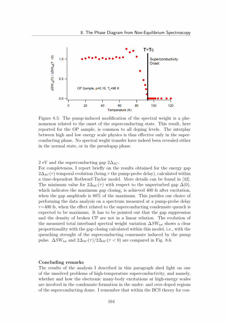
8. The Phase Diagram from Non-Equilibrium Spectroscopy
Figure 8.5: The pump-induced modification of the spectral weight is a phe-nomenon related to the onset of the superconducting state. This result, herereported for the OP sample, is common to all doping levels. The interplaybetween high and low energy scale physics is thus effective only in the super-conducting phase. No spectral weght transfer have indeed been revealed eitherin the normal state, or in the pseudogap phase.
2 eV and the superconducting gap 2∆SC .For completeness, I report briefly on the results obtained for the energy gap2∆SC(τ) temporal evolution (being τ the pump-probe delay), calculated withina time-dependent Rothwarf-Taylor model. More details can be found in [42].The minimum value for 2∆SC(τ) with respect to the unperturbed gap ∆(0),which indicates the maximum gap closing, is achieved 400 fs after excitation,when the gap amplitude is 80% of the maximum. This justifies our choice ofperforming the data analysis on a spectrum measured at a pump-probe delayτ=400 fs, when the effect related to the superconducting condensate quench isexpected to be maximum. It has to be pointed out that the gap suppressionand the density of broken CP are not in a linear relation. The evolution ofthe measured total interband spectral weight variation ∆SWtot shows a clearproportionality with the gap closing calculated within this model, i.e., with thequenching strenght of the superconducting consensate induced by the pumppulse. ∆SWtot and 2∆SC(τ)/2∆SC(τ < 0) are compared in Fig. 8.6.
Concluding remarksThe results of the analysis I described in this paragraph shed light on oneof the unsolved problems of high-temperature superconductivity, and namely,whether and how the electronic many-body excitations at high-energy scalesare involved in the condensate formation in the under- and over-doped regionsof the superconducting dome. I remember that within the BCS theory for con-
164
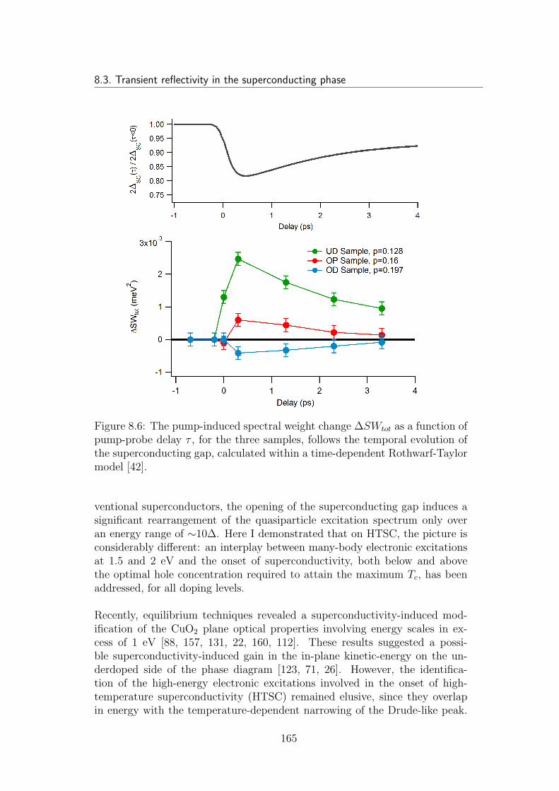
8.3. Transient reflectivity in the superconducting phase
Figure 8.6: The pump-induced spectral weight change ∆SWtot as a function ofpump-probe delay τ , for the three samples, follows the temporal evolution ofthe superconducting gap, calculated within a time-dependent Rothwarf-Taylormodel [42].
ventional superconductors, the opening of the superconducting gap induces asignificant rearrangement of the quasiparticle excitation spectrum only overan energy range of ∼10∆. Here I demonstrated that on HTSC, the picture isconsiderably different: an interplay between many-body electronic excitationsat 1.5 and 2 eV and the onset of superconductivity, both below and abovethe optimal hole concentration required to attain the maximum Tc, has beenaddressed, for all doping levels.
Recently, equilibrium techniques revealed a superconductivity-induced mod-ification of the CuO2 plane optical properties involving energy scales in ex-cess of 1 eV [88, 157, 131, 22, 160, 112]. These results suggested a possi-ble superconductivity-induced gain in the in-plane kinetic-energy on the un-derdoped side of the phase diagram [123, 71, 26]. However, the identifica-tion of the high-energy electronic excitations involved in the onset of high-temperature superconductivity (HTSC) remained elusive, since they overlapin energy with the temperature-dependent narrowing of the Drude-like peak.
165
8. The Phase Diagram from Non-Equilibrium Spectroscopy
The temporal-resolution provided by our non-equilibrium spectroscopy allowedto disentangle the ultrafast modifications of the high-energy spectral weight(∆SWtot ≡ ∆ω2
p,1/8 + ∆ω2p,2/8) from the slower broadening of the Drude-like
peak induced by the complete electron-boson thermalization. Time-resolvedoptical spectroscopy is thus one the most promising experimental techniquesto be used as a benchmark for unconventional models of HTSC.
Finally, these results shed light on the long-standing question [77, 52] aboutthe origin of the doping- and temperature-dependent ∆R/R(~ω = 1.55eV, τ)measured in one-colour time-resolved reflectivity experiments at high probe-energies [78, 117]. The measured signal is not originated by an excited stateabsorption, related to the variation of the electronic distribution within the un-varied electronic bands, but to a real modification of the underlying electronicstructure, and in particular, of the interband transitions at 1.5-2 eV. Nonethe-less, the measured ∆R/R(ω, τ) is proportional to the density of photo-injectedquasiparticles, as commonly assumed [111]. The dynamics of 2∆SC(τ) can thusbe reconstructed exploiting the ∆R/R(ω, τ) signal measured in the visible /near-IR spectral range.
8.4 Discontinuity of the dynamics at optimal
doping
In this paragraph, the change in the high-energy spectral weight determinedby the fitting procedure described in the previous section, will be related to thesuperconductivity-induced change in the carriers kinetic energy, in a few simplesteps I will sketch below. Fundamental information about the mechanismsleading to superconductivity will be argued. This will provide us fundamentalinformation in the attempt to formulate a ’non-equilibrium’ phase diagram.The conservation of the total spectral weight, imposed by the global oscillatorstrength sum rule (see section 3.6), implies that: SWN
D + SWNL = SW SC
D +SW SC
L , where the subscripts D and L indicate respectively the spectral weightof the intraband and interband regions, and the superscripts N , SC indicaterespectively the spectral weigth in the normal and superconducting phases.Here SW SC
D includes the contribution of the zero-frequency delta describingthe condensate contribution to the spectral weight.The total interband spectral weigth is given by (for either j = N or j = SC,and being (σL,i(ω))
j the optical conductivity of the i-th Lorentz oscillator inthe phase j):
SW jL ≡
∑
i
∫ ∞
0
(σL,i(ω))jdω
Similarly, for the intraband part, it holds:
SW jD ≡ (1/4πi)
∫ ∞
0
ω(ǫD(ω))jdω
166
8.4. Discontinuity of the dynamics at optimal doping
For the conservation of the total spectral weight, the spectral weight change ofthe intraband region must be compensated by an equal but opposite change ofthe spectral weight of the interband transitions. Moreover, since I did not ob-serve a superconductivity-induced modification of the high-energy oscillators,except the 1.5 and 2 eV ones, the following equalities hold (see also formula3.26):
∆SWD = −∆SWL = −∆ω2p,1/8−∆ω2
p,2/8
Where the ’∆’s I defined in this chapter follow in a natural way by consideringthe effect of the laser excitation on the system held in the superconductingphase, i.e., the partial suppression of the superconducting condensate. Since
∆R/R(ω, τ) ≡ Rpumped(ω,τ)−Runpumped(ω)
Runpumped(ω), it results: ∆ω2
p ≡ ω2p,pumped−ω2
p,unpumped
and ∆SWL = SWNL −SW SC
L . Since I want to estimate the superconductivity-induced spectral weigth change instead (N → SC), the correct quantity toconsider is −∆SWD = +∆SWL.In the special case of a single conduction band within the nearest-neighbourtight-binding model [86, 139], the total intraband spectral weight SWD can berelated to the kinetic energy Tδ of the charge carriers (holes) associated to anhopping process in the δ direction, through the relation [86]:
1
4πi
∫ ∞
0
ωǫD(ω)dω =π2a2δe
2
2~2VCu
〈−Tδ〉
where aδ is the lattice spacing in the Cu-O plane, projected along the directiondetermined by the in-plane polarization of the incident light, and VCu is thevolume per Cu atom. I obtain 〈K〉 = 2 〈Tδ〉 from the spectral weight variationof the interband oscillators, through the relation:
〈K〉 = 2 〈Tδ〉 =4~2VCu
π2a2δe2∆SWL
A finite value of ∆SWL thus implies a superconductivity-induced variation ofthe kinetic energy.To extract quantitative information about the actual superconductivity-inducedkinetic energy change, the values obtained for the kinetic energy change relatedto a pump fluence of 10 µJ/cm2, must be extrapolated to the case of a com-plete thermal collapse of the superconductive state (100% gap closing). Innon-equilibrium conditions, the collapse of the superconducting state happensfor a finite value of the superconductive gap 2∆, since the photoinduced phasetransition has a first order character, as predicted by the µeff model [143, 136],and clearly demonstrated in [42, 81]. The intuitive reason for this being the in-trinsic non-equilibrium character of the photoinduced phase transition, whichcannot be interpreted within equilibrium models, according to which the phasetransition happens only for a complete collapse of the superconducting gap 2∆.I thus estimated the actual density of broken CP (related to an incident fluenceof 10 µJ/cm2) starting from the knowledge of the critical CP density at which
167
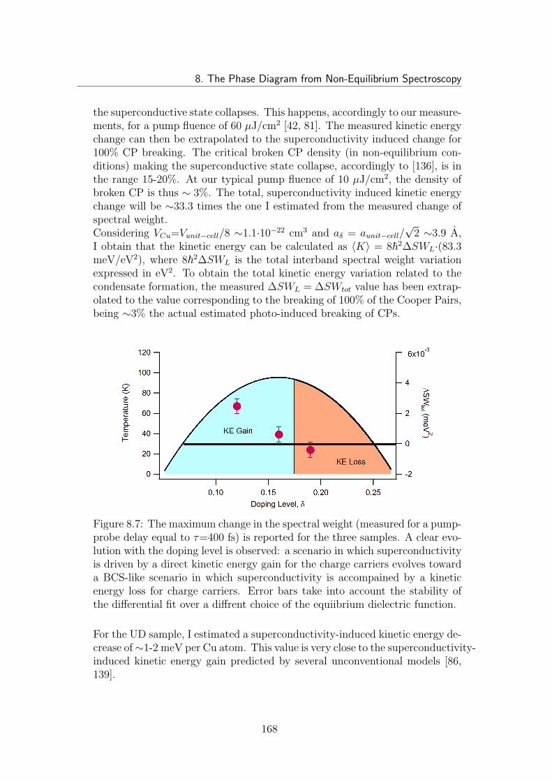
8. The Phase Diagram from Non-Equilibrium Spectroscopy
the superconductive state collapses. This happens, accordingly to our measure-ments, for a pump fluence of 60 µJ/cm2 [42, 81]. The measured kinetic energychange can then be extrapolated to the superconductivity induced change for100% CP breaking. The critical broken CP density (in non-equilibrium con-ditions) making the superconductive state collapse, accordingly to [136], is inthe range 15-20%. At our typical pump fluence of 10 µJ/cm2, the density ofbroken CP is thus ∼ 3%. The total, superconductivity induced kinetic energychange will be ∼33.3 times the one I estimated from the measured change ofspectral weight.Considering VCu=Vunit−cell/8 ∼1.1·10−22 cm3 and aδ = aunit−cell/
√2 ∼3.9 A,
I obtain that the kinetic energy can be calculated as 〈K〉 = 8~2∆SWL·(83.3meV/eV2), where 8~2∆SWL is the total interband spectral weight variationexpressed in eV2. To obtain the total kinetic energy variation related to thecondensate formation, the measured ∆SWL = ∆SWtot value has been extrap-olated to the value corresponding to the breaking of 100% of the Cooper Pairs,being ∼3% the actual estimated photo-induced breaking of CPs.
Figure 8.7: The maximum change in the spectral weight (measured for a pump-probe delay equal to τ=400 fs) is reported for the three samples. A clear evo-lution with the doping level is observed: a scenario in which superconductivityis driven by a direct kinetic energy gain for the charge carriers evolves towarda BCS-like scenario in which superconductivity is accompained by a kineticenergy loss for charge carriers. Error bars take into account the stability ofthe differential fit over a diffrent choice of the equiibrium dielectric function.
For the UD sample, I estimated a superconductivity-induced kinetic energy de-crease of∼1-2 meV per Cu atom. This value is very close to the superconductivity-induced kinetic energy gain predicted by several unconventional models [86,139].
168
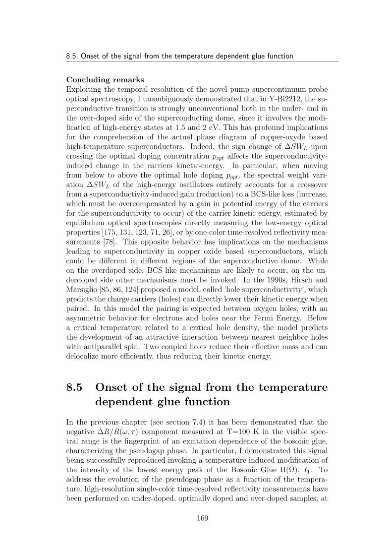
8.5. Onset of the signal from the temperature dependent glue function
Concluding remarksExploiting the temporal resolution of the novel pump supercontinuum-probeoptical spectroscopy, I unambiguously demonstrated that in Y-Bi2212, the su-perconductive transition is strongly unconventional both in the under- and inthe over-doped side of the superconducting dome, since it involves the modi-fication of high-energy states at 1.5 and 2 eV. This has profound implicationsfor the comprehension of the actual phase diagram of copper-oxyde basedhigh-temperature superconductors. Indeed, the sign change of ∆SWL uponcrossing the optimal doping concentration popt affects the superconductivity-induced change in the carriers kinetic-energy. In particular, when movingfrom below to above the optimal hole doping popt, the spectral weight vari-ation ∆SWL of the high-energy oscillators entirely accounts for a crossoverfrom a superconductivity-induced gain (reduction) to a BCS-like loss (increase,which must be overcompensated by a gain in potential energy of the carriersfor the superconductivity to occur) of the carrier kinetic energy, estimated byequilibrium optical spectroscopies directly measuring the low-energy opticalproperties [175, 131, 123, 71, 26], or by one-color time-resolved reflectivity mea-surements [78]. This opposite behavior has implications on the mechanismsleading to superconductivity in copper oxide based superconductors, whichcould be different in different regions of the superconductive dome. Whileon the overdoped side, BCS-like mechanisms are likely to occur, on the un-derdoped side other mechanisms must be invoked. In the 1990s, Hirsch andMarsiglio [85, 86, 124] proposed a model, called ’hole superconductivity’, whichpredicts the charge carriers (holes) can directly lower their kinetic energy whenpaired. In this model the pairing is expected between oxygen holes, with anasymmetric behavior for electrons and holes near the Fermi Energy. Belowa critical temperature related to a critical hole density, the model predictsthe development of an attractive interaction between nearest neighbor holeswith antiparallel spin. Two coupled holes reduce their effective mass and candelocalize more efficiently, thus reducing their kinetic energy.
8.5 Onset of the signal from the temperature
dependent glue function
In the previous chapter (see section 7.4) it has been demonstrated that thenegative ∆R/R(ω, τ) component measured at T=100 K in the visible spec-tral range is the fingerprint of an excitation dependence of the bosonic glue,characterizing the pseudogap phase. In particular, I demonstrated this signalbeing successfully reproduced invoking a temperature induced modification ofthe intensity of the lowest energy peak of the Bosonic Glue Π(Ω), I1. Toaddress the evolution of the pseudogap phase as a function of the tempera-ture, high-resolution single-color time-resolved reflectivity measurements havebeen performed on under-doped, optimally doped and over-doped samples, at
169
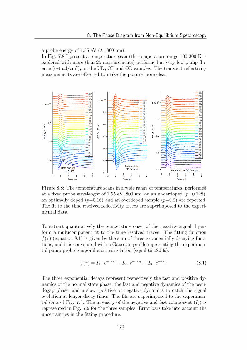
8. The Phase Diagram from Non-Equilibrium Spectroscopy
a probe energy of 1.55 eV (λ=800 nm).In Fig. 7.8 I present a temperature scan (the temperature range 100-300 K isexplored with more than 25 measurements) performed at very low pump flu-ence (∼4 µJ/cm2), on the UD, OP and OD samples. The transient reflectivitymeasurements are offsetted to make the picture more clear.
Figure 8.8: The temperature scans in a wide range of temperatures, performedat a fixed probe wavelenght of 1.55 eV, 800 nm, on an underdoped (p=0.128),an optimally doped (p=0.16) and an overdoped sample (p=0.2) are reported.The fit to the time resolved reflectivity traces are superimposed to the experi-mental data.
To extract quantitatively the temperature onset of the negative signal, I per-form a multicomponent fit to the time resolved traces. The fitting functionf(τ) (equation 8.1) is given by the sum of three exponentially-decaying func-tions, and it is convoluted with a Gaussian profile representing the experimen-tal pump-probe temporal cross-correlation (equal to 180 fs).
f(τ) = I1 · e−τ/τ1 + I2 · e−τ/τ2 + I3 · e−τ/τ3 (8.1)
The three exponential decays represent respectively the fast and positive dy-namics of the normal state phase, the fast and negative dynamics of the pseu-dogap phase, and a slow, positive or negative dynamics to catch the signalevolution at longer decay times. The fits are superimposed to the experimen-tal data of Fig. 7.8. The intensity of the negative and fast component (I2) isrepresented in Fig. 7.9 for the three samples. Error bars take into account theuncertainties in the fitting procedure.
170
8.5. Onset of the signal from the temperature dependent glue function
Figure 8.9: The intensity of the negative component I2, extracted from thefit, is reported. The onset of the negative signal associated to an impulsivequench of the lowest-energy peak of the bosonic glue has been inferred fromthese data. Error bars take into account the fit uncertainty.
It is evident how the onset of this effect is rather narrow in temperature: 150to 165 K for the OP sample, 230 to 240 K for the UD sample. Moreover,this onset temperature scales with doping. No negative component has beendetected on the OD sample.
Summarizing, our findings clearly show that for UD and OP samples a negativecomponent in the ∆R/R(ω, τ) appears at a temperature which is compatiblewith the material T ∗. The onset of this effect is doping-dependent, and scales asT ∗ does. This negative component is absent in the OD sample. This negativecomponent in the ∆R/R(ω, τ) has been successfully reproduced (see section7.4) assuming that one peak in the material Bosonic Glue Π(Ω) depends onthe excitation, that is, it is temperature dependent. Electron-Boson couplingis thus no-more temperature-independent in the pseudogap.As I carefully stated in section 7.4, Li et al. [116] revealed, on the HgBa2CuO4+δ
copper-oxyde based high-temperature superconductor, a collective magneticmode of excitation (with energy in the range ∼55 meV), which onset tem-perature shows a temperature evolution similar to that observed in our time-resolved optical data.Our analysis indicates that the scenario of a temperature independent GlueFunction must be overcame to correctly reproduce the experimentl results ob-tained in the pseudogap phase. Provided that the feature we observed in thebosonic glue is in a relation with the magnetic mode observed by Li et al. (asit is reasonable to assume), we can say that not only a new magnetic exci-tation mode appears at T ∗, but it turns out that this peculiar mode is also
171
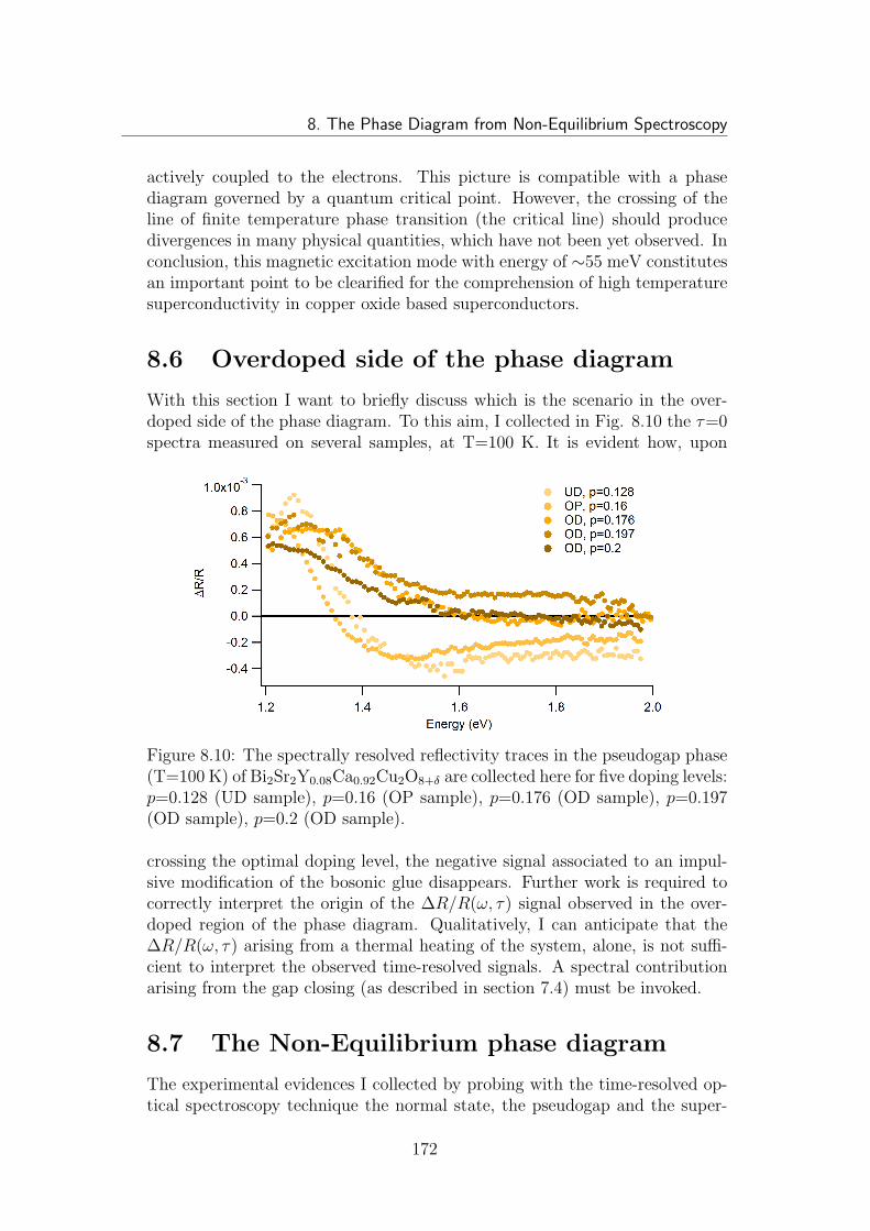
8. The Phase Diagram from Non-Equilibrium Spectroscopy
actively coupled to the electrons. This picture is compatible with a phasediagram governed by a quantum critical point. However, the crossing of theline of finite temperature phase transition (the critical line) should producedivergences in many physical quantities, which have not been yet observed. Inconclusion, this magnetic excitation mode with energy of ∼55 meV constitutesan important point to be clearified for the comprehension of high temperaturesuperconductivity in copper oxide based superconductors.
8.6 Overdoped side of the phase diagram
With this section I want to briefly discuss which is the scenario in the over-doped side of the phase diagram. To this aim, I collected in Fig. 8.10 the τ=0spectra measured on several samples, at T=100 K. It is evident how, upon
Figure 8.10: The spectrally resolved reflectivity traces in the pseudogap phase(T=100 K) of Bi2Sr2Y0.08Ca0.92Cu2O8+δ are collected here for five doping levels:p=0.128 (UD sample), p=0.16 (OP sample), p=0.176 (OD sample), p=0.197(OD sample), p=0.2 (OD sample).
crossing the optimal doping level, the negative signal associated to an impul-sive modification of the bosonic glue disappears. Further work is required tocorrectly interpret the origin of the ∆R/R(ω, τ) signal observed in the over-doped region of the phase diagram. Qualitatively, I can anticipate that the∆R/R(ω, τ) arising from a thermal heating of the system, alone, is not suffi-cient to interpret the observed time-resolved signals. A spectral contributionarising from the gap closing (as described in section 7.4) must be invoked.
8.7 The Non-Equilibrium phase diagram
The experimental evidences I collected by probing with the time-resolved op-tical spectroscopy technique the normal state, the pseudogap and the super-
172
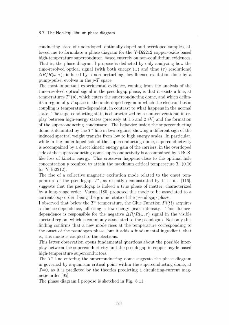
8.7. The Non-Equilibrium phase diagram
conducting state of underdoped, optimally-doped and overdoped samples, al-lowed me to formulate a phase diagram for the Y-Bi2212 copper-oxide basedhigh-temperature supercondutor, based enterely on non-equilibrium evidences.That is, the phase diagram I propose is deducted by only analyzing how thetime-resolved optical signal (with both energy (ω) and time (τ) resolutions)∆R/R(ω, τ), induced by a non-perturbing, low-fluence excitation done by apump-pulse, evolves in the p-T space.The most important experimental evidence, coming from the analysis of thetime-resolved optical signal in the pseudogap phase, is that it exists a line, attemperatures T ∗(p), which enters the superconducting dome, and which delim-its a region of p-T space in the underdoped region in which the electron-bosoncoupling is temperature-dependent, in contrast to what happens in the normalstate. The superconducting state is characterized by a non-conventional inter-play between high-energy states (precisely at 1.5 and 2 eV) and the formationof the superconducting condensate. The behavior inside the superconductingdome is delimited by the T ∗ line in two regions, showing a different sign of theinduced spectral weight transfer from low to high energy scales. In particular,while in the underdoped side of the superconducting dome, superconductivityis accompained by a direct kinetic energy gain of the carriers, in the overdopedside of the superconducting dome superconductivity is accompained by a BCS-like loss of kinetic energy. This crossover happens close to the optimal holeconcentration p required to attain the maximum critical temperature Tc (0.16for Y-Bi2212).The rise of a collective magnetic excitation mode related to the onset tem-perature of the pseudogap, T ∗, as recently demonstrated by Li et al. [116],suggests that the pseudogap is indeed a true phase of matter, characterizedby a long-range order. Varma [180] proposed this mode to be associated to acurrent-loop order, being the ground state of the pseudogap phase.I observed that below the T ∗ temperature, the Glue Function Pi(Ω) acquiresa fluence-dependence, affecting a low-energy peak intensity. This fluence-dependence is responsible for the negative ∆R/R(ω, τ) signal in the visiblespectral region, which is commonly associated to the pseudogap. Not only thisfinding confirms that a new mode rises at the temperature corresponding tothe onset of the pseudogap phase, but it adds a fundamental ingredient, thatis, this mode is coupled to the electrons.This latter observation opens fundamental questions about the possible inter-play between the superconductivity and the pseudogap in copper-oxyde basedhigh-temperature superconductors.The T ∗ line entering the superconducting dome suggests the phase diagramin governed by a quantum critical point within the superconducting dome, atT=0, as it is predicted by the theories predicting a circulating-current mag-netic order [95].The phase diagram I propose is sketched in Fig. 8.11.
173
8. The Phase Diagram from Non-Equilibrium Spectroscopy
Figure 8.11: The phase diagram I propose, based enterely on the non-equilibrium evidences from the time-resolved optical spectroscopy, is sketched.Red line delimits the superconducting dome. Blue line is the T ∗ line, related tothe onset of the pseudogap. This line delimits a region in which the electron-boson coupling is fluence-dependent. The yellow square and the green dotrepresent respectively the onset temperature of the fluence-dependence of theelectron-boson coupling, for the p=0.128 (UD) and the p=0.16 (OP) samples.Entering the superconducting dome, superconductivity is accompained by adoping-dependent change of the carriers kinetic energy, that changes sign closeto the optimal doping concentration.
174
Chapter 9Conclusions
My PhD work started with the task of developing and setting up novel time-resolved spectroscopies, with the idea that only the knowledge of the non-equilibrium optical response of complex materials, in a wide range of energies,could lead to a true comprehension of the physics at the microscopic level,originating the non-equilibrium optical signal. We brought a fundamental con-tribution to this nascent field, actively developing the basis for this approach,which is nowadays achieving great success and is quickly spreading aroundthe time resolved scientific community. Many difficulties had to be overcome,mainly related to the need to obtain a very high sensitivity for the measure-ments, related to the fact that phases of matter which ’vaporizes’ at very lowfluence levels had to be investigated. This is the peculiarity of our approach:the systems under study are only gently brought out-of-equilibrium by laserexcitation. In this respect we call our technique time-resolved spectroscopy,since a true spectroscopic analysis of the phase can be achieved only whenthe phase itself is not ’vaporized’. Temporal resolution allowed to reveal thecharacteristic non-equilibrium optical response to a small perturbation of thephase, which strongly depends on the ground state of the system.In the specific, I developed two complementary experimental set-ups. The firstexploits a broadband, supercontinuum white light pulse as probe pulse. Thespectral range that can be probed by this setup is 1.2-2.5 eV (i.e., 500-1000nm). The supercontinuum pulse employed in this set-up is generated by aphotonic crystal fiber, which is seeded by a cavity-dumped Ti:Sapphire oscil-lator. This allowed to obtain very high signal-to-noise ratios, thanks to thehigh statistic due to the high repetition rate of the source. The drawback hasbeen that the temporal structure of pulses produced in this way presents a pro-nounced chirp, and this lead us to the development of several characterizationtechniques to measure the spectro-temporal structure of this pulse, and correctmeasurements accordingly. The second setup is developed around an opticalparametric amplifier, seeded by a regenerative amplified laser system. Theprobe pulse of this setup is a quasi-monochromatic but widely tunable infraredpulse, obtained as the signal and idler output of the parametric amplifier. This
175
9. Conclusions
technique allowed us to extend the probed spectral range toward the infrared,covering the spectral region 0.5-1 eV (i.e., 1200-2400 nm). The two set-upsdeveloped, together with a brief review of the characterization techniques, arepresented in chapter 5. After some years these systems have been working, it ispossible to say that time and spectral resolved measurements constitute a fun-damental improvement over the conventional one color, monochromatic opticalpump-probe techniques. Up to now, the lack of spectral resolution preventedto achieve a true comprehension of the physical origin of the observed opticalsignals. Other improvements can be done to the technique, mainly related tothe extension of the probed spectral range. For the systems studied in thiswork, the infrared part of the spectrum revealed of greater relevance as com-pared to the ultraviolet one. Extending the probed spectral range toward theinfrared is however not simple, because of the actual lack of broadband sources,except for the THz range. Also the achievement of even better signal-to-noiseratios is important, to perform measurements more quickly, thus opening theway to follow the signal evolution in time. This would be extremely useful tomap for example the evolution of chemical reactions from the non-equilibriumpoint of view. In the field of strongly correlated electron systems (transitionmetal oxides, copper and iron based superconductors) or other complex mate-rials (manganites, ruthenates), time-resolved spectroscopy is one of the mostpromising techniques to provide new insights on the microscopic mechanismsunderlying the phases of these materials and new benchmarks for the non-equilibrium theories which are being developed.
With regard to my research, this novel powerful technique allowed to clarifysome open questions about the physics of copper oxide based high temper-ature superconductors. The sample chosen is the two-layer member of theYttrium substituted BSCCO family, that is, Bi2Sr2Ca0.92Y0.08Cu2O8+δ, whereδ controls the doping level. We have samples with different doping, in sucha way we could explore the evolution of the non-equilibrium optical signalin the δ-T phase diagram. The analysis and characterization - by the non-equilibrium spectroscopic point of view - of the phases composing the systemphase diagram, allowed us to obtain the first all-optical non equilibrium phasediagram of a strongly-correlated electronic material. In particular, the normalstate, the pseudogap and the superconducting state exhibited sensibly differ-ent time-resolved optical signals. These non-equilibrium spectrally resolvedsignals have been interpreted within a differential dielectric function approach(formulated and described in chapter 4), to assign a clear microscopic origin tothe signal itself. When excited by an ultrashort laser pulse, each physical phasemanifests a peculiar, intrinsic response, mainly due to the excitations producedby the pulse, which are meaningful in understanding the ground state of thephase. Each physical mechanism has its own spectral fingerprint, as it has beendemonstrated with several simulations. Moreover, the temporal resolution re-vealed fundamental since it allows to disentangle the fast electronic processes
176
from the slow, thermal (phonon related) ones. The thermal contribution oftenoverwhelms the signal of electronic origin. This is the reason why equilibriumspectroscopy failed in evidencing the effects revealed by the non-equilibriumapproach.
Briefly, what we found about the microscopic nature of the normal (Chap-ter 6), pseudogap (Chapter 7) and superconducting (Chapter 8) phases can besummarized as follows:
• The time-resolved optical signal measured by time-resolved spectroscopyin the normal state of Y-Bi2212, unambiguously revealed that, after atime shorter than the electron-phonon thermalization, the electrons arealready thermalized with some bosonic degrees of freedom, having a smallspecific heat and a strong coupling with the electrons. This finding sug-gests that these bosonic excitations are of electronic origin. The time-resolved optical signal in the energy domain is only compatible with aquasi-thermal scenario, in which electrons are never decoupled from aboson subset. The simultaneous analysis of experimental data in boththe time and the energy domains revealed that the subset of bosonicexcitations of electronic origin can account, alone, for the high criticaltemperature of the material. This finding suggests that pairing in HTSCis mainly of electronic origin. Possible candidates for the bosons of elec-tronic origin are antiferromagnetic spin flucutations or current loops. Inthe normal state, the Bosonic Glue Π(Ω) expressing electron-boson cou-pling is fluence-independent.
• In the pseudogap phase the transient reflectivity signal requires a morecomplicated explanation. It is doping dependent, in contrast to the nor-mal state signal. A quasi-thermal scenario, alone, is not enough forexplaining the observed signal. The further contributions which has tobe invoked to correctly reproduce the time-resolved optical signal arethe pump-induced impulsive quench of a gap in the electronic density ofstates, and the impulsive decrease of the intensity of one low-energy peakof the Bosonic Glue Π(Ω). The onset of this fluence-dependent contri-bution, which is responsible for the negative signal commonly associatedto the presence of the pseudogap phase, is exactly at T ∗. These exper-imental observations suggest that in the pseudogap phase one bosonicmode, rising exactly at T ∗, is also coupled with the electron system.The pseudogap phase is thus a complex phase, in which the fermionicquasi-particles and the bosonic excitations are strongly intertwined. Thedoping-dependent temperature onset of the effect related to the fluence-dependence of the electron-boson coupling allowed to formulate the phasediagram of the Y-Bi2212 compound.
• The superconducting state shows a very peculiar optical response with re-spect to an external excitation by ultrashort laser pulses. The main effect
177
9. Conclusions
of the excitation is to partially quench (working in a low fluence regime)the superconducting gap. On the contrary to what happens in BCS, con-ventional superconductors, in which the effect on the optical propertiesof the superconducting gap is limited in a spectral range very close tothe gap itself, in strongly correlated copper oxide based superconductors,an effect at energies much higher than the gap energy is observed in theoptical properties. It exists an interplay between high and low energyphysics. Some high energy states, and the relevant optical transitions,are intimately related to the condensate formation. In contrast to whatobserved in the normal state and in the pseudogap phases, here the time-resolved optical signal, which shows a strong doping dependence, can beinterpreted only by invoking a pump-induced modification of two Lorentzoscillators at 1.5 and 2 eV, which are present in the equilibrium dielectricfunction and associated to transitions between many-body Cu-O states.The superconducting signal exhibits a strong doping dependence, fromwhich useful information about the superconductivity driving mechanismcan be extracted. Close to the optimal doping level required to attainthe highest Tc, a crossover from a direct kinetic energy gain in the un-derdoped side of the phase diagram to a BCS like kinetic energy loss inthe overdoped side of the phase diagram is observed.
All the reported findings can be matched to provide a phase diagram enterelybased on all-optical non-equilibrium evidences. The scenario proposed is thatof a phase diagram governed by a quantum critical point at T=0, locatedinside the superconducting dome. A line entering the superconducting domedelimits the pseudogap behavior associated to a fluence-dependent electron-boson coupling. This evidence suggests the pseudogap is indeed a true phaseof matter. The T ∗ line delimits, within the superconducting dome, two regionsin which superconductivity is accompained by an opposite superconductivity-induced change for the carriers kinetic energy.
178
Bibliography
[1] S. Johnston et al. Evidence for forward scattering and couplingto acoustic phonon modes in high-Tc cuprate superconductors.arXiv:1101.1302v1 (2011).
[2] A. Abanov, A. V. Chubukov, and J. Schmalian. Fingerprints of spinmediated pairing in cuprates. J. Electron Spectrosc. Relat. Phenom.,117:129, 2001.
[3] R. R. Alfano and S. L. Shapiro. Emission in the region 4000 to 7000 Avia four-photon coupling in glass. Phys. Rev. Lett., 24:584, 1970.
[4] R. R. Alfano and S. L. Shapiro. Observation of self-phase modulationand small-scale filaments in crystals and glasses. Phys. Rev. Lett., 24:592,1970.
[5] J. W. Allen and J. C. Mikkelsen. Optical properties of CrSb, MnSb,NiSb, NiAs. Phys. Rev. B, 15:2952, 1977.
[6] P. B. Allen. Electron-phonon effects in the infrared properties of metals.Phys. Rev. B, 3:305, 1971.
[7] P. B. Allen. Theory of thermal relaxation of electrons in metals. Phys.Rev. Lett., 59:1460, 1987.
[8] P. B. Allen and R.C. Dynes. Transition temperature of strong-coupledsuperconductors reanalyzed. Phys. Rev. B, 12:905, 1975.
[9] P. W. Anderson. Is There Glue in Cuprate Superconductors? Science,316:1705, 2007.
[10] S. I. Anisimov, B. L. Kapeliovich, and T. L. Perel’man. Electron emissionfrom metal surfaces exposed to ultrashort laser pulses. Zh. Eksp. Teor.Fiz., 66:776, 1974.
[11] N. W. Ashcroft and N. D. Mermin. Solid state physics. Harcourt CollegePublishers, Orlando FL, 1976.
179
BIBLIOGRAPHY
[12] R. D. Averitt, G. Rodriguez, A. I. Lobad, J. W. L. Siders, S. L. Trugman,and A. J. Taylor. Nonequilibrium superconductivity and quasiparticledynamics in YBa2Cu3O7−δ. Phys. Rev. B, 63:140502.
[13] J. Bardeen, L. N. Cooper, and J. R. Schrieffer. Microscopic Theory ofSuperconductivity. Phys. Rev., 106:162, 1957.
[14] J. Bardeen, L. N. Cooper, and J. R. Schrieffer. Theory of Superconduc-tivity. Phys. Rev., 108:1175, 2008.
[15] D. N. Basov and T. Timusk. Electrodynamics of high-Tc superconduc-tors. Rev. Mod. Phys., 77:721, 2005.
[16] D.N. Basov, R.D. Averitt, D. van der Marel, M. Dressel, and K. Haule.Electrodynamics of Correlated Electron Materials. Rev. Mod. Phys.,83:471, 2011.
[17] M. Bassi, P. Camagni, R. Rolli, G. Samoggia, F. Parmigiani,G. Dhalenne, and A. Revcolevschi. Optical absorption of CuGeO3. Phys.Rev. B, 54.
[18] B. Batlogg, H. Y. Hwang, H. Takagi, R. J. Cava, H. L. Kao, and J. Kwo.Normal state phase diagram of (La,Sr)2CuO4 from charge and spin dy-namics. Physica C, 130:235, 1994.
[19] M. Beck, M. Klammer, S. Lang, P. Leiderer, V. V. Kabanov, G. N.Goltsman, and J. Demsar. Energy-gap dynamics of superconductingNbN thin films studied by time-resolved terahertz spectroscopy. ArXive,1102.
[20] M. Beck, H. Schafer, G. Klatt, J. Demsar, S. Winnerl, M. Helm, andT. Dekorsy. Impulsive terahertz radiation with high electric fields froman amplifier-driven large-area photoconductive antenna. Opt. Express,18:9251, 2010.
[21] J. G. Bednorz and K. A. Muller. Possible high Tc superconductivity inthe Ba-La-Cu-O system. Z. Phys. B: Condens. Matter, 64:189, 1986.
[22] A. V. Boris, N. N. Kovaleva, O. V. Dolgov, T. Holden, C. T. Lin,B. Keimer, and C. Bernhard. In-plane spectral weight shift of chargecarriers in yba2cu3o6.9. Science, 304:708, 2004.
[23] N. B. Brookes, G. Ghiringhelli, O. Tjernberg, L. H. Tjeng, T. Mizokawa,T. W. Li, and A. A. Menovsky. Detection of Zhang-Rice Singlets UsingSpin-Polarized Photoemission. Phys. Rev. Lett., 87:237003, 2001.
[24] S. D. Brorson, A. Kazeroonian, D. W. Face, T. K. Cheng, G. L. Doll,M. S. Dresselhaus, G. Dresselhaus, E. P. Ippen, T. Venkatesan, X. D.
180
BIBLIOGRAPHY
Wu, and A. Inam. Femtosecond thermomodulation study of high-tc su-perconductors. Solid State Commun., 74:1305, 1990.
[25] S. D. Brorson, A. Kazeroonian, J. S. Moodera, D. W. Face, T. K. Cheng,E. P. Ippen, M. S. Dresselhaus, and G. Dresselhaus. Femtosecond room-temperature measurement of the electron-phonon coupling constant γ inmetallic superconductors. Phys. Rev. Lett., 64:2172, 1990.
[26] F. Carbone, A. B. Kuzmenko, H. J. A. Molegraaf, E. van Heumen,V. Lukovac, F. Marsiglio, and D. van der Marel. Doping dependence ofthe redistribution of optical spectral weight in Bi2Sr2CaCu2O8+δ. Phys.Rev. B, 74:064510, 2006.
[27] F. Carbonea, D.-S. Yanga, E. Giannini, and A. H. Zewail. Direct roleof structural dynamics in electron-lattice coupling of superconductingcuprates. Proc. Natl. Acad. Sci., 105:20161, 2008.
[28] J. P. Carbotte. Properties of boson-exchange superconductors. Rev.Mod. Phys., 62:1027, 1990.
[29] A. Cavalleri, H. H. W. Chong, S. Fourmaux, T. E. Glover, P. A. Heimann,J. C. Kieffer, B. S. Mun, H. A. Padmore, and R. W. Schoenlein. Picosec-ond soft x-ray absorption measurement of the photoinduced insulator-to-metal transition in VO2. Phys. Rev. B, 69:153106, 2004.
[30] A. Cavalleri, Th. Dekorsy, H. H. W. Chong, J. C. Kieffer, and R. W.Schoenlein. Evidence for a structurally-driven insulator-to-metal tran-sition in VO2: A view from the ultrafast timescale. Phys. Rev. B,70:161102.
[31] A. Cavalleri, C. Toth, C. W. Siders, J. A. Squier, F. Raksi, P. Forget,and J. C. Kieffer. Femtosecond Structural Dynamics in VO2 during anUltrafast Solid-Solid Phase Transition. Phys. Rev. Lett., 87:237401, 2001.
[32] Tsuei CC. Phys. Rev. Lett., 73:593, 1994.
[33] S. Chakravarty, R. B. Laughlin, D. K. Morr, and C. Nayak. Hidden orderin the cuprates. Phys. Rev. B, 63:094503, 2001.
[34] Han-Yong Choi, C. M. Varma, and Xingjiang Zhou. Superconductivityin the Cuprates: Deduction of Mechanism for D-Wave Pairing ThroughAnalysis of ARPES. ArXive, 1110.
[35] A. V. Chubukov and J Schmalian. Superconductivity due to masslessboson exchange in the strong-coupling limit. Phys. Rev. B, 72:174520,2005.
181
BIBLIOGRAPHY
[36] Ye Chuntang, Yang Jilian, Zhang Baisheng, Li Jizhou, Kang Jian, JinLan, Ding Yongfan, He Yusheng, Zhang Jincang, He Aisheng, and XiangJiong. Structure Refinement of Bi2Sr1.855Ca1.145Cu2O8 from NeutronData. Chin. Phys. Lett., 8:521, 1991.
[37] F. Cilento, C. Giannetti, G. Ferrini, S. Dal Conte, T. Sala, G. Coslovich,M. Rini, A. Cavalleri, and F. Parmigiani. Ultrafast insulator-to-metalphase transition as a switch to measure the spectrogram of a supercon-tinuum light pulse. Appl. Phys. Lett., 96:021102, 2010.
[38] S. Dal Conte. Time-resolved optical spectroscopy onBi2Sr2Ca0.92Y0.08Cu2O8+δ. PhD thesis, Universita degli Studi diPavia, March 2011.
[39] B. R. Cooper, H. Ehrenreich, and H. R. Philipp. Optical Properties ofNoble Metals. II. Phys. Rev., 138:494, 1965.
[40] Leon N. Cooper. Bound Electron Pairs in a Degenerate Fermi Gas. Phys.Rev., 104:1189, 1956.
[41] R. Cortes, L. Rettig, Y. Yoshida, H. Eisaki, M. Wolf, and U. Bovensiepen.Momentum-Resolved Ultrafast Electron Dynamics in SuperconductingBi2Sr2CaCu2O8. ArXive, 1011.
[42] G. Coslovich, C. Giannetti, F. Cilento, S. Dal Conte, G. Ferrini,P. Galinetto, M. Greven, H. Eisaki, M. Raichle, R. Liang, A. Dam-ascelli, and F. Parmigiani. Evidence for a photoinduced nonther-mal superconducting-to-normal-state phase transition in overdopedbi2sr2ca0.92y0.08cu2o8+δ. Phys. Rev. B, 83:064519, 2011.
[43] M. F. Crommie and A. Zettl. Thermal-conductivity anisotropy of single-crystal Bi2Sr2CaCu2O8. Phys. Rev. B, 43:408, 1991.
[44] T. Cuk, D. H. Lu, X. J. Zhou, Z.-X. Shen, T. P. Devereaux, and N. Na-gaosa. A review of electron-phonon coupling seen in the high-Tc su-perconductors by angle-resolved photoemission studies (ARPES). Phys.Stat. Sol. b, 242:11, 2005.
[45] Wollman DA. Phys. Rev. Lett., 71:2134, 1993.
[46] E. Dagotto. Correlated electrons in high-temperature superconductors.Rev. Mod. Phys., 66:763, 1994.
[47] T. Dahm, V. Hinkov, S. V. Borisenko, A. A. Kordyuk, V. B. Zabolot-nyy, J. Fink, B. Buchner, D. J. Scalapino, W. Hanke, and B. Keimer.Strength of the Spin-Fluctuation-Mediated Pairing Interaction in a High-Temperature Superconductor. ArXive, 0812.
182
BIBLIOGRAPHY
[48] T. Dahm, V. Hinkov, S. V. Borisenko, A.A. Kordyuk, V.B. Zabolot-nyy, J. Fink, B. Buchner, D.J. Scalapino, W. Hanke, and B. Keimer.Strength of the spin-fluctuation-mediated pairing interaction in a high-temperature superconductor. Nature Physics, 5:217, 2009.
[49] A. Damascelli, Z. Hussain, and Z.-X. Shen. Angle-resolved photoemissionstudies of the cuprate superconductors. Rev. Mod. Phys., 75:473, 2003.
[50] Johnston DC. Phys. Rev. Lett., 62:957, 1989.
[51] L. de Medici, X. Wang, M. Capone, and A. J. Millis. Correlationstrength, gaps, and particle-hole asymmetry in high-Tc cuprates: A dy-namical mean field study of the three-band copper-oxide model. Phys.Rev. B, 77:014518, 2009.
[52] J. Demsar, R. A. Averitt, V. V. Kabanov, and D. Mihailovic. Com-ment on Photoinduced Changes of Reflectivity in Single Crystals ofYBa2Cu3O6.5 (Ortho II). Phys. Rev. Lett., 91:169701, 2003.
[53] J. Demsar, B. Podobnik, V. V. Kabanov, T. Wolf, and D. Mihailovic. Su-perconducting Gap ∆c, the Pseudogap ∆p, and Pair Fluctuations aboveTc in Overdoped Y1−xCaxBa2Cu3O7−δ from Femtosecond Time-DomainSpectroscopy. Phys. Rev. Lett., 82:4918, 1999.
[54] J. Demsar, J. L. Sarrao, and A. J. Taylor. Dynamics of photoexcitedquasiparticles in heavy electron compounds. J. Phys.:Condens. Matter,18, 2006.
[55] G. Deutscher. Coherence in High Temperature Superconductors. WorldScientific, 1995.
[56] T.P. Devereaux, T. Cuk, Z.-X. Shen, and N. Nagaosa. AnisotropicElectron-Phonon Interaction in the Cuprates. Phys. Rev. Lett.,93:117004, 2004.
[57] A. L. Dobryakov, V. M. Farztdinov, Y. E. Lozovik, and V. S. Letokhov.Energy gap in the superconductor optical spectrum. J. Am. Chem. Soc,105:309, 1994.
[58] P. Domachuk, N. A. Wolchover, M. Cronin-Golomb, A. Wang, A. K.George, C. M. B. Cordeiro, J. C. Knight, and F. G. Omenetto. Over 4000nm Bandwidth of Mid-IR Supercontinuum Generation in sub-centimeterSegments of Highly Nonlinear Tellurite PCFs. Opt. Express, 16:7161,2008.
[59] M. Dressel and G. Grunner. Electrodynamics of solids: optical propertiesof electrons in matter. Cambridge University Press, Cambridge, 2002.
183
BIBLIOGRAPHY
[60] G. Dresselhaus and M. S. Dresselhaus. Interband transitions in super-conductors. Phys. Rev., 125:1212, 1962.
[61] J. M. Dudley, G. Genty, and S. Coen. Supercontinuum generation inphotonic crystal fiber. Rev. Mod. Phys., 78:1135, 2006.
[62] R. Dynes. . Solid State Commun., 10:615, 1972.
[63] G. L. Eesley. Observation of Nonequilibrium Electron Heating in Copper.Phys. Rev. Lett., 51:2140, 1983.
[64] G. L. Eesley. Generation of nonequilibrium electron and lattice tem-peratures in copper by picosecond laser pulses. Phys. Rev. B, 33:2144,1986.
[65] H. Ehrenreich and H. R. Philipp. Optical Properties of Ag and Cu. Phys.Rev., 128:1622, 1962.
[66] H. Ehrenreich, H. R. Philipp, and D. J. Olechna. Optical Properties andFermi Surface of Nickel. Phys. Rev., 131:2469, 1963.
[67] H. Ehrenreich, H. R. Philipp, and B. Segall. Optical Properties of Alu-minum. Phys. Rev., 132:1918, 1963.
[68] H. Eisaki, N. Kaneko, D. L. Feng, A. Damascelli, P. K. Mang, K. M.Shen, Z.-X. Shen, and M. Greven. Effect of chemical inhomogeneity inbismuth-based copper oxide superconductors. Phys. Rev. B, 69:064512,2004.
[69] G. M. Eliashberg. Sov. Phys. JEPT, 11:696, 1960.
[70] V. J. Emery and S. A. Kivelson. Importance of phase fluctuation insuperconductors with small superfluid density. Nature, 374:4347, 1995.
[71] G. Deutscher et al. Kinetic energy change with doping upon super-fluid condensation in high-temperature superconductors. Phys. Rev. B,72:092504, 2005.
[72] N. B. Brookes et al. A determination of the pairing interaction in thehigh Tc cuprate superconductor T l2Ba2CaCu2O8 (Tl2212). Physica C,40:460, 2007.
[73] B. Fauque, Y. Sidis, V. Hinkov, S. Pailhes, C. T. Lin2, X. Chaud, andP. Bourges. Magnetic order in the pseudogap phase of high-Tc super-conductors. Phys. Rev. Lett., 96:197001, 2006.
[74] D. Fournier, G. Levy, Y. Pennec, J.L. McChesney, A. Bostwick, E. Roten-berg, R. Liang, W.N. Hardy, D.A. Bonn, I.S. Elfimov, and A. Damascelli.Loss of nodal quasiparticle integrity in underdoped YBa2Cu3O6+x. Na-ture Physics, 6:905, 2010.
184
BIBLIOGRAPHY
[75] C Gadermaier, A Alexandrov, V Kabanov, P Kusar, T Mertelj, X Yao,C Manzoni, D Brida, G Cerullo, and D Mihailovic. Electron-PhononCoupling in High-Temperature Cuprate Superconductors Determinedfrom Electron Relaxation Rates. Phys. Rev. Lett., 105(25), December2010.
[76] C Gadermaier, A Alexandrov, V Kabanov, P Kusar, T Mertelj, X Yao,C Manzoni, D Brida, G Cerullo, and D Mihailovic. Electron-PhononCoupling in High-Temperature Cuprate Superconductors Determinedfrom Electron Relaxation Rates. Supplementary material. Phys. Rev.Lett., 105(25), December 2010.
[77] N. Gedik, P. Blake, R. C. Spitzer, J. Orenstein, R. Liang, D. A. Bonn,and W. N. Hardy. Single-quasiparticle stability and quasiparticle-pairdecay in YBa2Cu3O6.5. Phys. Rev. B, 70:014504, 2004.
[78] N. Gedik, M. Langner, J. Orenstein, S. Ono, Y. Abe, and Y. Ando.Abrupt Transition in Quasiparticle Dynamics at Optimal Doping in aCuprate Superconductor System. Phys. Rev. Lett., 95:117005, 2005.
[79] N. Gedik, J. Orenstein, R. Liang, D. A. Bonn, and W. N. Hardy. Gediket al. Reply:. Phys. Rev. Lett., 91:169702, 2003.
[80] C. Giannetti, F. Cilento, S. Dal Conte, G. Coslovich, G. Ferrini, H. Mole-graaf, M. Raichle, R. Liang, H. Eisaki, M. Greven, A. Damascelli,D. van der Marel, and F. Parmigiani. Revealing the high-energy elec-tronic excitations underlying the onset of high-temperature supercon-ductivity in cuprates. Nature Communications, 3:253, 2011.
[81] C. Giannetti, G. Coslovich, F. Cilento, G. Ferrini, H. Eisaki, N. Kaneko,M. Greven, and F. Parmigiani. Discontinuity of the ultrafast electronicresponse of underdoped superconducting Bi2Sr2CaCu2O8+δ strongly ex-cited by ultrashort light pulses. Phys. Rev. B, 79:224502, 2009.
[82] C. Giannetti, G. Zgrablic, C. Consani, A. Crepaldi, D. Nardi, G. Ferrini,G. Dhalenne, A. Revcolevschi, and F. Parmigiani. Disentangling thermaland nonthermal excited states in a charge-transfer insulator by time- andfrequency-resolved pump-probe spectroscopy. Phys. Rev. B, 80:235129,2009.
[83] Alloul H. Phys. Rev. Lett., 63:1700, 1989.
[84] E. Hecht. Optics. Addison Wesley, 2002.
[85] J. E. Hirsch and F. Marsiglio. Superconducting state in an oxygen holemetal. Phys. Rev. B, 39:11515, 1989.
185
BIBLIOGRAPHY
[86] J. E. Hirsch and F. Marsiglio. Optical sum rule violation, superfluidweight, and condensation energy in the cuprates. Phys. Rev. B, 62:15131,2000.
[87] J. Hohlfeld, S.-S. Wellershoff, J. Gudde, U. Conrad, V. Jahnke, andE. Matthias. Electron and lattice dynamics following optical excitationof metals. Chem. Phys., 251:237, 2000.
[88] M. J. Holcomb, J. P. Collman, and W. A. Little. Optical evidence ofan electronic contribution to the pairing interaction in superconductingTl2Ba2Ca2Cu3O10.Phys.Rev.Lett., 73 : 2360, 1994.
[89] S. Hufner, M. A. Hossain, A. Damascelli, and G. A. Sawatzky. Two gapsmake a high-temperature superconductor? Rep. Prog. Phys, 71:062501,2008.
[90] J. Hwang. Electron-boson spectral density function of underdopedBi2Sr2CaCu2O8 and YBa2Cu3O6.50. Phys. Rev. B, 83:014507, 2011.
[91] J. Hwang, T. Timusk, and G. D. Gu. High-transition-temperature su-perconductivity in the absence of the magnetic-resonance mode. Nature,427:714, 2007.
[92] J. Hwang, T. Timusk, E. Schachinger, and J. P. Carbotte. Evolutionof the bosonic spectral density of the high-temperature superconductorbi2sr2cacu2o8+δ. Phys. Rev. B, 75:144508, 2007.
[93] W. Rudolph J. C. Diels. Ultrashort Laser Pulse Phenomena. AcademicPress, 1996.
[94] A. Junod, K.-Q. Wang, T. Tsukamoto, G. Triscone, B. Revaz, E. Walker,and J. Muller. Specific heat up to 14 tesla and magnetization of aBi2Sr2CaCu2O8 single crystal. Thermodynamics of a 2D superconduc-tor. Physica C, 229:209, 1994.
[95] A. Junod, K.-Q. Wang, T. Tsukamoto, G. Triscone, B. Revaz, E. Walker,and J. Muller. Non-Fermi-liquid states and pairing instability of a generalmodel of copper oxide metals. Phys. Rev. B, 55:14554, 1997.
[96] V. V. Kabanov and A. S. Alexandrov. Electron relaxation in metals:Theory and exact analytical solutions. Phys. Rev. B, 78:174514, 2008.
[97] V. V. Kabanov, J. Demsar, B. Podobnik, and D. Mihailovic. Quasiparti-cle relaxation dynamics in superconductors with different gap structures:Theory and experiments on YBa2Cu3O7−δ. Phys. Rev. B, 59:1497, 1999.
[98] V. V. Kabanov and J. Demsarand D. Mihailovic. Kinetics of a Super-conductor Excited with a Femtosecond Optical Pulse. Phys. Rev. Lett.,95:147002, 2005.
186
BIBLIOGRAPHY
[99] R. A. Kaindl, M. A. Carnahan, D. S. Chemla, S. Oh, and J. N. Eckstein.Dynamics of Cooper pair formation in Bi2Sr2CaCu2O8+δ. Phys. Rev. B,72:060510, 2005.
[100] R. A. Kaindl, F. Eickemeyer, M. Woerner, and T. Elsaesser. Broad-band phase-matched difference frequency mixing of femtosecond pulsesin GaSe: Experiment and theory. Appl. Phys. Lett., 75:1060, 1999.
[101] R. A. Kaindl, D. C. Smith, M. Joschko, M. P. Hasselbeck, M. Woerner,and T. Elsaesser. Femtosecond infrared pulses tunable from 9 to 18 µmat an 88-MHz repetition rate. Opt. Lett., 23:861, 1998.
[102] R. A. Kaindl, M. Woerner, T. Elsaesser, D. C. Smith, J. F. Ryan, G. A.Farnan, M. P. McCurry, and D. G. Walmsley. Ultrafast mid-infraredresponse of YBa2Cu3O7−δ. Science, 287:470, 2000.
[103] Yoichi Kamihara, Hidenori Hiramatsu, Masahiro Hirano, Ryuto Kawa-mura, Hiroshi Yanagi, Toshio Kamiya, and Hideo Hosono. Iron-BasedLayered Superconductor:a LaOFeP. J. Am. Chem. Soc, 128:10012, 2006.
[104] A. Kaminski, H. M. Fretwell, M. R. Norman, M. Randeria,S. Rosenkranz, U. Chatterjee, J. C. Campuzano, J. Mesot, T. Sato,T. Takahashi, T. Terashima, M. Takano, K. Kadowaki, Z. Z. Li, andH. Raffy. Momentum anisotropy of the scattering rate in cuprate super-conductors. Chem. Phys., 71:014517, 2005.
[105] H. J. Kaufmann, E. G. Maksimov, and E. K. H. Salje. Electron-PhononInteraction and Optical Spectra of Metals. Journal of Superconductivity,11:755, 1998.
[106] Jae Hun Kim, Meng-Ku Chen, Chia-En Yang, Jon Lee, Stuart (Shizhuo)Yin, Paul Ruffin, Eugene Edwards, Christina Brantley, and Claire Luo.Broadband IR supercontinuum generation using single crystal sapphirefibers. Opt. Express, 16:4085, 2008.
[107] J. C. Knight. Photonic crystal fibres. Nature, 424:847, 2003.
[108] N.N. Kovaleva, A.V. Boris, T. Holden, C. Ulrich, B. Liang, C.T. Lin,B. Keimer, C. Bernhard, J.L. Tallon, D. Munzar, and A.M. Stoneham.c-axis lattice dynamics in Bi-based cuprate superconductors. Phys. Rev.B, 69:054511, 2004.
[109] Todd D. Krauss and Frank W. Wise. Femtosecond measurement of non-linear absorption and refraction in CdS, ZnSe, and ZnS. Appl. Phys.Lett., 65:1739, 1994.
[110] V.Z. Kresin and S.A. Wolf. Colloquium: Electron-lattice interaction andits impact on high Tc superconductivity. Rev. Mod. Phys., 81:481, 2009.
187
BIBLIOGRAPHY
[111] P. Kusar, V.V. Kabanov, J. Demsar, T. Mertelj, S. Sugai, and D. Mi-hailovic. Controlled Vaporization of the Superconducting Condensate inCuprate Superconductors by Femtosecond Photoexcitation. Phys. Rev.Lett., 101:227001, 2008.
[112] A. B. Kuzmenko, H. J. A. Molegraaf, F. Carbone, and D. van der Marel.Temperature-modulation analysis of superconductivity-induced transferof in-plane spectral weight in bi2sr2cacu2o8. Phys. Rev. B, 72:144503,2005.
[113] A. Lanzara, P. V. Bogdanov, X. J. Zhou, S. A. Kellar, D. L. Feng, E. D.Lu, T. Yoshida, H. Eisaki, A. Fujimori, K. Kishio, J.-I. Shimoyama,T. Noda, S. Uchida, Z. Hussain, and Z.-X. Shen. Evidence for ubiquitousstrong electron-phonon coupling in high-temperature superconductors.Nature, 412:510, 2001.
[114] Jinho Lee, K. Fujita, K. McElroy, J. A. Slezak, M. Wang, Y. Aiura,H. Bando, M. Ishikado, T. Masui, J.-X. Zhu, A. V. Balatsky, H. Eisaki,S. Uchida, and J. C. Davis. Interplay of electron-lattice interactions andsuperconductivity in Bi2Sr2CaCu2O8+δ. Nature, 442:546, 2006.
[115] Y. Li, V. Baledent, N. Barisic, Y. Cho, B. Fauque, Y. Sidis, G. Yu,X. Zhao, P. Bourges, and M. Greven. Unusualmagnetic order in the pseu-dogap region of the superconductor HgBa2CuO4+δ. Nature, 455:372,2008.
[116] Y. Li, V. Baledent, G.Yu, N. Barisic, K. Hradil, R. A. Mole, Y. Sidis,P. Steffens, X. Zhao, P. Bourges, and M. Greven. Hidden magneticexcitation in the pseudogap phase of a high-Tc superconductor. Nature,468:283, 2010.
[117] Y. H. Liu, Y. Toda, K. Shimatake, N. Momono, and M. Odaand M. Ido.Direct Observation of the Coexistence of the Pseudogap and Supercon-ducting Quasiparticles in Bi2Sr2CaCu2O8+y by Time-Resolved OpticalSpectroscopy. Phys. Rev. Lett., 101:137003, 2008.
[118] J. W. Loram, J. L. Luo, J. R. Cooper, W. Y. Liang, and J. L. Tallon.The Condensation Energy and Pseudogap Energy Scale of Bi2212 fromthe Electronic Specific Heat. J. Phys. Chem., 62:59, 2001.
[119] J. W. Loram, K. A. Mirza, J. R. Cooper, and J. L. Tallon. Specific heatevidence on the normal state pseudogap. J. Phys. Chem. Sol., 59:2091,1998.
[120] E. G. Maksimov. High-temperature superconductivity: the current state.Physics Uspekhi, 43:965, 2000.
188
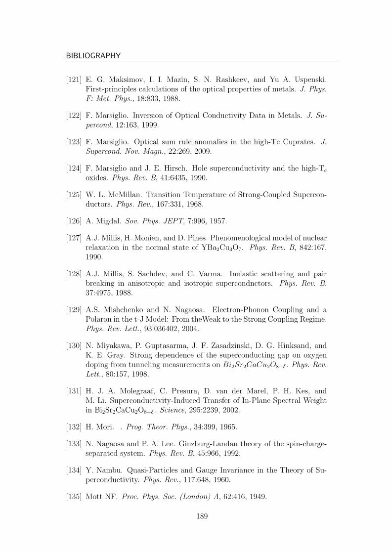
BIBLIOGRAPHY
[121] E. G. Maksimov, I. I. Mazin, S. N. Rashkeev, and Yu A. Uspenski.First-principles calculations of the optical properties of metals. J. Phys.F: Met. Phys., 18:833, 1988.
[122] F. Marsiglio. Inversion of Optical Conductivity Data in Metals. J. Su-percond, 12:163, 1999.
[123] F. Marsiglio. Optical sum rule anomalies in the high-Tc Cuprates. J.Supercond. Nov. Magn., 22:269, 2009.
[124] F. Marsiglio and J. E. Hirsch. Hole superconductivity and the high-Tc
oxides. Phys. Rev. B, 41:6435, 1990.
[125] W. L. McMillan. Transition Temperature of Strong-Coupled Supercon-ductors. Phys. Rev., 167:331, 1968.
[126] A. Migdal. Sov. Phys. JEPT, 7:996, 1957.
[127] A.J. Millis, H. Monien, and D. Pines. Phenomenological model of nuclearrelaxation in the normal state of YBa2Cu3O7. Phys. Rev. B, 842:167,1990.
[128] A.J. Millis, S. Sachdev, and C. Varma. Inelastic scattering and pairbreaking in anisotropic and isotropic supercondnctors. Phys. Rev. B,37:4975, 1988.
[129] A.S. Mishchenko and N. Nagaosa. Electron-Phonon Coupling and aPolaron in the t-J Model: From theWeak to the Strong Coupling Regime.Phys. Rev. Lett., 93:036402, 2004.
[130] N. Miyakawa, P. Guptasarma, J. F. Zasadzinski, D. G. Hinksand, andK. E. Gray. Strong dependence of the superconducting gap on oxygendoping from tunneling measurements on Bi2Sr2CaCu2O8+δ. Phys. Rev.Lett., 80:157, 1998.
[131] H. J. A. Molegraaf, C. Presura, D. van der Marel, P. H. Kes, andM. Li. Superconductivity-Induced Transfer of In-Plane Spectral Weightin Bi2Sr2CaCu2O8+δ. Science, 295:2239, 2002.
[132] H. Mori. . Prog. Theor. Phys., 34:399, 1965.
[133] N. Nagaosa and P. A. Lee. Ginzburg-Landau theory of the spin-charge-separated system. Phys. Rev. B, 45:966, 1992.
[134] Y. Nambu. Quasi-Particles and Gauge Invariance in the Theory of Su-perconductivity. Phys. Rev., 117:648, 1960.
[135] Mott NF. Proc. Phys. Soc. (London) A, 62:416, 1949.
189
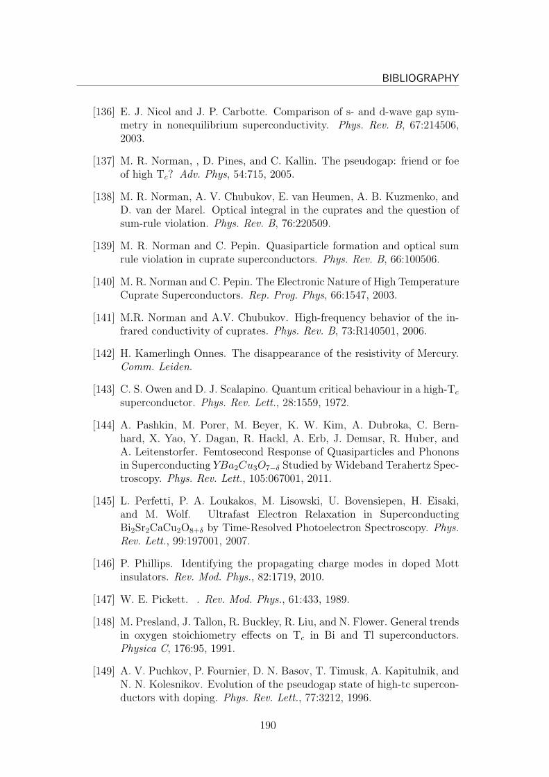
BIBLIOGRAPHY
[136] E. J. Nicol and J. P. Carbotte. Comparison of s- and d-wave gap sym-metry in nonequilibrium superconductivity. Phys. Rev. B, 67:214506,2003.
[137] M. R. Norman, , D. Pines, and C. Kallin. The pseudogap: friend or foeof high Tc? Adv. Phys, 54:715, 2005.
[138] M. R. Norman, A. V. Chubukov, E. van Heumen, A. B. Kuzmenko, andD. van der Marel. Optical integral in the cuprates and the question ofsum-rule violation. Phys. Rev. B, 76:220509.
[139] M. R. Norman and C. Pepin. Quasiparticle formation and optical sumrule violation in cuprate superconductors. Phys. Rev. B, 66:100506.
[140] M. R. Norman and C. Pepin. The Electronic Nature of High TemperatureCuprate Superconductors. Rep. Prog. Phys, 66:1547, 2003.
[141] M.R. Norman and A.V. Chubukov. High-frequency behavior of the in-frared conductivity of cuprates. Phys. Rev. B, 73:R140501, 2006.
[142] H. Kamerlingh Onnes. The disappearance of the resistivity of Mercury.Comm. Leiden.
[143] C. S. Owen and D. J. Scalapino. Quantum critical behaviour in a high-Tc
superconductor. Phys. Rev. Lett., 28:1559, 1972.
[144] A. Pashkin, M. Porer, M. Beyer, K. W. Kim, A. Dubroka, C. Bern-hard, X. Yao, Y. Dagan, R. Hackl, A. Erb, J. Demsar, R. Huber, andA. Leitenstorfer. Femtosecond Response of Quasiparticles and Phononsin Superconducting YBa2Cu3O7−δ Studied byWideband Terahertz Spec-troscopy. Phys. Rev. Lett., 105:067001, 2011.
[145] L. Perfetti, P. A. Loukakos, M. Lisowski, U. Bovensiepen, H. Eisaki,and M. Wolf. Ultrafast Electron Relaxation in SuperconductingBi2Sr2CaCu2O8+δ by Time-Resolved Photoelectron Spectroscopy. Phys.Rev. Lett., 99:197001, 2007.
[146] P. Phillips. Identifying the propagating charge modes in doped Mottinsulators. Rev. Mod. Phys., 82:1719, 2010.
[147] W. E. Pickett. . Rev. Mod. Phys., 61:433, 1989.
[148] M. Presland, J. Tallon, R. Buckley, R. Liu, and N. Flower. General trendsin oxygen stoichiometry effects on Tc in Bi and Tl superconductors.Physica C, 176:95, 1991.
[149] A. V. Puchkov, P. Fournier, D. N. Basov, T. Timusk, A. Kapitulnik, andN. N. Kolesnikov. Evolution of the pseudogap state of high-tc supercon-ductors with doping. Phys. Rev. Lett., 77:3212, 1996.
190
BIBLIOGRAPHY
[150] Anderson PW. Solid State Phys., 14:99, 1963.
[151] Anderson PW. Science, 235:1196, 1987.
[152] J. K. Ranka, R. S. Windeler, and A. J. Stentz. Visible continuum genera-tion in air-silica microstructure optical fibers with anomalous dispersionat 800 nm. Opt. Lett., 25:25, 2000.
[153] Ch. Renner, B. Revaz, J.-Y. Genoud, K. Kadowaki, and A. Fischer. Pseu-dogap Precursor of the Superconducting Gap in Under- and OverdopedBi2Sr2CaCu2O8. Phys. Rev. Lett., 80:149, 1998.
[154] M. Rini, Z. Hao, R. W. Schoenlein, C. Giannetti, F. Parmigiani, S. Four-maux, J. C. Kieffer, A. Fujimori, M. Onoda, S. Wall, and A. Cavalleri.Optical switching in VO2 films by below-gap excitation. Appl. Phys.Lett., 92:181904, 2008.
[155] P. Romaniello, P. L. de Boeij, F. Carbone, and D. van der Marel. Opticalproperties of bcc transition metals in the range 0a40 eV. Phys. Rev. B,73:075115, 2006.
[156] A. Rothwarf and B. N. Taylor. Measurements of recombination lifetimesin superconductors. Phys. Rev. Lett., 19:27, 1967.
[157] M. Rubhausen, A. Gozar, M. V. Klein, P. Guptasarma, and D. G. Hinks.Superconductivity-induced optical changes for energies of 100∆ in thecuprates. Phys. Rev. B, 63:224514, 2001.
[158] J. C. Russell. Photonic crystal fibers. Science, 299:358, 2003.
[159] G Sangiovanni, O Gunnarsson, E Koch, C Castellani, and M Capone.Electron-Phonon Interaction and Antiferromagnetic Correlations. Phys.Rev. Lett., 97(4), July 2006.
[160] A. F. Santander-Syro, R. P. S. M. Lobo, N. Bontemps, W. Lopera, D. Gi-rata, Z. Konstantinovic, Z. Z. Li, and H. Raffy. In-plane electrodynamicsof the superconductivity in Bi2Sr2CaCu2O8: Energy scales and spectralweight distribution. Phys. Rev. B, 70:134504, 2004.
[161] G. A. Sawatzky and J. W. Allen. . Phys. Rev. Lett., 53:2339, 1984.
[162] D. J. Scalapino, E. Loh, and J. E. Hirsch. d-wave pairing near a spin-density-wave instability. Phys. Rev. B, 34:8190, 1986.
[163] R. W. Schoenlein, W. Z. Lin, J. G. Fujimotor, and G. L. Eesley. Fem-tosecond Studies of Nonequilibrium Electronic Processes in Metals. Phys.Rev. Lett., 58:1680, 1987.
191
BIBLIOGRAPHY
[164] G. P. Segre, N. Gedik, J. Orenstein, D. A. Bonn, R. Liang, and W. N.Hardy. Photoinduced Changes of Reflectivity in Single Crystals ofYBa2Cu3O6.5 (Ortho II). Phys. Rev. Lett., 82:3054, 2002.
[165] C. V. Shank, R. Yen, and C. Hirlimann. Time-Resolved ReflectivityMeasurements of Femtosecond-Optical-Pulse-Induced Phase Transitionsin Silicon. Phys. Rev. Lett., 50:454, 1983.
[166] S. G. Sharapov and J. P. Carbotte. Effects of energy dependence in thequasiparticle density of states on far-infrared absorption in the pseudogapstate. Phys. Rev. B, 72:134506, 2005.
[167] S.V. Shulga, O. V. Dolgov, and E. G. Maksimov. Electronic statesand optical spectra of HTSC with electron-phonon coupling. PhysicaC, 178:266, 1991.
[168] L. Stojchevska, P. Kusar, T. Mertelj, V. V. Kabanov, Y. Toda, X. Yao,and D. Mihailovic. Mechanisms of nonthermal destruction of the super-conducting state and melting of the charge-density-wave state by fem-tosecond laser pulses. ArXive, 1109.
[169] S.Wall, D. Brida, S. R. Clark, H. P. Ehrke, D. Jaksch, A. Arda-van, S. Bonora, H. Uemura, Y. Takahashi, T. Hasegawa, H. Okamoto,G. Cerullo, and A. Cavalleri. Quantum interference between charge ex-citation paths in a solid-state Mott insulator. Nature Physics, 7:114,2011.
[170] M. Le Tacon, G. Ghiringhelli, J. Chaloupka, M. Moretti Sala, V. Hinkov,M.W. Haverkort, M. Minola, M. Bakr, K. J. Zhou, S. Blanco-Canosa,C. Monney, Y. T. Song, G. L. Sun, C. T. Lin, G. M. De Luca, M. Sal-luzzo, G. Khaliullin, T. Schmitt, L. Braicovich, and B. Keimer. Intenseparamagnon excitations in a large family of high-temperature supercon-ductors. Nature Physics, 7:725, 2011.
[171] Louis Taillefer. Scattering and Pairing in Cuprate Superconductors.Annu. Rev. Condens. Matter Phys., 1:51, 2010.
[172] H. J. Tao, F. Lu, and E. J. Wolf. Observation of pseudogap inBi2Sr2CaCu2O8+δ single crystals with electron tunneling spectroscopy.Physica C, 282:1507, 1997.
[173] T. Timusk and B. Statt. The pseudogap in high-temperature supercon-ductors: an experimental survey. Rep. Prog. Phys, 62:61, 1999.
[174] T. Timusk and D. B. Tanner. Physical Properties of High TemperatureSuperconductors I. World Scientific, Singapore, 1989.
[175] M. Tinkham. Introduction to superconductivity. McGraw-Hill, New York,1975.
192
[176] R. Trebino. Frequency-Resolved Optical Gating: The Measurement ofUltrashort Laser Pulses. Springer, New York, 2002.
[177] T. Valla, A. V. Fedorov, J. Lee, J. C. Davis, and G. D. Gu. The groundstate of the pseudogap in cuprate superconductors. Science, 314:1914,2006.
[178] D. van der Marel, H. J. A. Molegraaf, J. Zaanen, Z. Nussinov, F. Car-bone, A. Damascelli, H. Eisaki, M. Greven, P. H. Kes, and M. Li. Quan-tum critical behaviour in a high-Tc superconductor. Nature, 425:271,2003.
[179] E. van Heumen, E. Muhlethaler, A. B. Kuzmenko, H. Eisaki,W. Meevasana, M. Greven, and D. van der Marel. Optical determi-nation of the relation between the electron-boson coupling function andthe critical temperature in high-Tc cuprates. Phys. Rev. B, 79:184512,2009.
[180] C. Varma. Mind the pseudogap. Nature.
[181] C. M. Varma. Pseudogap Phase and the Quantum-Critical Point inCopper-Oxide Metals. Phys. Rev. Lett., 83:3538, 1999.
[182] C.M. Varma. Theory of the pseudogap state of the cuprates. Phys. Rev.B, 73:155113, 2006.
[183] L. Vidmar, J. Bonca, T. Tohyama, and S. Maekawa. Quantum Dynamicsof a Driven Correlated System Coupled to Phonons. Phys. Rev. Lett.,107:246404, 2011.
[184] D. Wegkamp, D. Brida, S. Bonora, G. Cerullo, J. Stahler, M. Wolf, andS. Wall. Phase retrieval and compression of low-power white-light pulses.Appl. Phys. Lett., 99:101101, 2011.
[185] F. Wooten. Optical properties of solids. Academic Press, New-York,1972.
[186] Warren WW. Phys. Rev. Lett., 62:1193, 1989.
[187] G. Yu, E. M. Motoyama, and M. Greven. A universal relationship be-tween magnetic resonance and superconducting gap in unconventionalsuperconductors. Nature Physics, 5:873, 2009.
[188] F.C. Zhang and T. Rice. Effective Hamiltonian for the superconductingCu oxides. Phys. Rev. B, 37:3759, 1988.
193

194
List of publications
• C. Giannetti, F. Cilento, S. Dal Conte, G. Coslovich, G. Ferrini, H. Mole-graaf, M. Raichle, R. Liang, H. Eisaki, M. Greven, A. Damascelli, D. vander Marel, and F. ParmigianiRevealing the high-energy electronic excitations underlying the onset ofhigh-temperature superconductivity in cupratesNature Communications 2, 353 (2011) and http://arxiv.org/abs/1105.2508
• G. Coslovich, C. Giannetti, F. Cilento, S. Dal Conte, G. Ferrini, P.Galinetto, M. Greven, H. Eisaki, M. Raichle, R. Liang, A. Damascelli,and F. ParmigianiEvidence for a photoinduced nonthermal superconducting-to-normal-statephase transition in overdoped Bi2Sr2Ca0.92Y0.08Cu2O8+d by ultrashortlaser pulsesPhys. Rev. B 83, 052907 (2011) and http://arxiv.org/abs/1005.4320
• G. Galimberti, S. Pagliara, S. Ponzoni, S. Dal Conte, F. Cilento, G.Ferrini, S. Hofmann, M. Arshad, C. Cepek, and F. ParmigianiThe photoinduced charge transfer mechanism in aligned and unalignedcarbon nanotubesCarbon 49, 5246 (2011)
• F. Cilento, C. Giannetti, G. Ferrini, S. Dal Conte, T. Sala, G. Coslovich,M. Rini, A. Cavalleri, and F. ParmigianiUltrafast insulator-to-metal phase transition as a switch to measure thespectrogram of a supercontinuum light pulseAppl. Phys. Lett. 96, 021102 (2010) and http://arxiv.org/abs/0910.3785
• G. Coslovich, C. Giannetti, F. Cilento, G. Ferrini, and F. ParmigianiQuasi-particles dynamics in underdoped Bi2212 under strong optical per-turbationAIP Conference Proceedings 1162, pp. 177-185 (2009)
• C. Giannetti, G. Coslovich, F. Cilento, G. Ferrini, H. Eisaki, N. Kaneko,M. Greven, and F. Parmigiani
195
Discontinuity of the ultrafast electronic response of underdoped supercon-ducting Bi2 Sr2CaCu2O8+d strongly excited by ultrashort light pulsesPhys. Rev. B 79, 224502 (2009) and http://arxiv.org/abs/0804.4822This paper was selected for the Virtual Journal of Applications of Su-perconductivity.This paper was selected for the Virtual Journal of Ultrafast Science.
• C. Giannetti, B. Revaz, F. Banfi, M. Montagnese, G. Ferrini, F. Cilento,S. Maccalli, P. Vavassori, G. Oliviero, E. Bontempi, L.E. Depero, V.Metlushko, and F. ParmigianiThermo-mechanical behavior of surface acoustic waves in ordered arraysof nanodisks studied by near infrared pump-probe diffraction experimentsPhys. Rev. B 76, 125413 (2007) and http://arxiv.org/abs/cond-mat/0701666This paper was selected for the Virtual Journal of Nanoscale ScienceTechnology.This paper was selected for the Virtual Journal of Ultrafast Science.
Submitted or In preparation
• S. Dal Conte, C. Giannetti, G. Coslovich, F. Cilento, D. Bossini, T.Abebaw, F. Banfi, G. Ferrini, H. Eisaki, M. Greven, A. Damascelli, D.van der Marel, and F. ParmigianiDisentangling the electronic and phononic glue in a high-Tc supercon-ductorAccepted for Publication on Science (February 2012)
• G. Coslovich, C. Giannetti, F. Cilento, S. Dal Conte, G. Ferrini, M.Raichle, R. Liang, A. Damascelli, and F. ParmigianiThe relation between pseudogap and superconductivity: Causality or Ca-sualty?
• F. Cilento, C. Giannetti, S. Dal Conte, G. Coslovich, A. Damascelli, andF. ParmigianiPseudogap Phase: temperature dependent glue function
• F. Cilento, C. Giannetti, S. Dal Conte, G. Coslovich, A. Damascelli, andF. ParmigianiNon-equilibrium phase diagram of Bi2212 cuprate superconductors re-vealed by ultrafast optical spectroscopy
196
Ringraziamenti
I want to end this work with some acknowledgments. First of all, I wantto thank my supervisor, Prof. Fulvio Parmigiani, who stimulated and madepossible this project. I thank all the people working in the T-ReX Group inTrieste, and in the Ultrafast Group in Brescia. A special thank to ClaudioGiannetti, who constitutes a reference for me since many years. He thougthand supervised this complex research project with enthusiasm, professionalityand patience, coordinating a team of young researchers. I want in particular tothank Stefano dal Conte and Giacomo Coslovich, as component of this team.With them I spent a significative and pleasant part of my PhD. The amountof data and models presented in this work are also the result of their scientificefforts. Thanks also to Prof. Andrea Damascelli for providing samples, and toProf. Dirk van der Marel for providing the static optical data.
197