Teoria da probabilidade - ULisboa of the form Λ∩F,where F∈F ... Teoria da probabilidade...
159
Teoria da probabilidade Teacher: Patr´ ıcia Gon¸ calves Tutor: Ragaa Ahmed Patr´ ıciaGon¸calves (IST Lisbon) Teoria da probabilidade 2016/2017 1 / 159
Transcript of Teoria da probabilidade - ULisboa of the form Λ∩F,where F∈F ... Teoria da probabilidade...
Teoria da probabilidade
Teacher: Patrıcia GoncalvesTutor: Ragaa Ahmed
Patrıcia Goncalves (IST Lisbon) Teoria da probabilidade 2016/2017 1 / 159

Set theory TP 2016/2017
Set theory
Patrıcia Goncalves (IST Lisbon) Teoria da probabilidade 2016/2017 2 / 159
Set theory TP 2016/2017
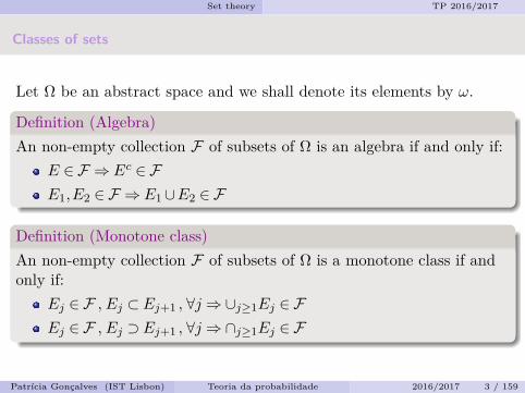
Classes of sets
Let Ω be an abstract space and we shall denote its elements by ω.
Definition (Algebra)An non-empty collection F of subsets of Ω is an algebra if and only if:
E ∈ F ⇒ Ec ∈ FE1,E2 ∈ F ⇒ E1∪E2 ∈ F
Definition (Monotone class)An non-empty collection F of subsets of Ω is a monotone class if andonly if:
Ej ∈ F , Ej ⊂ Ej+1 , ∀j⇒∪j≥1Ej ∈ FEj ∈ F , Ej ⊃ Ej+1 , ∀j⇒∩j≥1Ej ∈ F
Patrıcia Goncalves (IST Lisbon) Teoria da probabilidade 2016/2017 3 / 159
Set theory TP 2016/2017
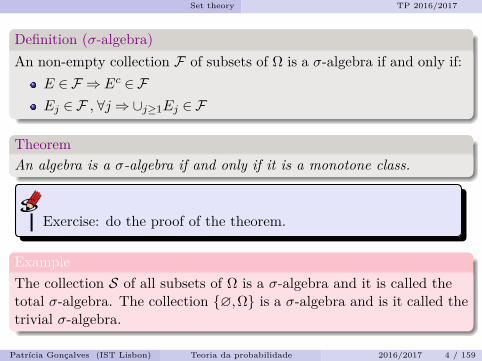
Definition (σ-algebra)An non-empty collection F of subsets of Ω is a σ-algebra if and only if:
E ∈ F ⇒ Ec ∈ FEj ∈ F , ∀j⇒∪j≥1Ej ∈ F
TheoremAn algebra is a σ-algebra if and only if it is a monotone class.
Exercise: do the proof of the theorem.
ExampleThe collection S of all subsets of Ω is a σ-algebra and it is called thetotal σ-algebra. The collection ∅,Ω is a σ-algebra and is it called thetrivial σ-algebra.
Patrıcia Goncalves (IST Lisbon) Teoria da probabilidade 2016/2017 4 / 159
Set theory TP 2016/2017
Remark1 If A is an index set and if for α ∈A, Fα is a σ-algebra (or a
monotone class), then ∩α∈AFα is a σ-algebra (or a monotoneclass).
2 Given a non empty collection of sets C, there exists a minimalσ-algebra (or algebra or monotone class) containing C, whichconsists in the intersection of all σ-algebras (or algebras ormonotone classes) containing C. It is the minimal σ-algebra S.This σ-algebra (or algebra or monotone class) is called theσ-algebra generated by C.
TheoremLet F0 be an algebra, C the minimal monotone class containing F0 andF the minimal σ-algebra containing F0. Then F = C.
Exercise: do the proof of the theorem.
Patrıcia Goncalves (IST Lisbon) Teoria da probabilidade 2016/2017 5 / 159
Probability measure TP 2016/2017
Probability measures and distribution functions
Patrıcia Goncalves (IST Lisbon) Teoria da probabilidade 2016/2017 6 / 159
Probability measure TP 2016/2017
Probability measure
DefinitionLet Ω be an abstract space and F a σ-algebra of subsets of Ω. Aprobability measure P(·) in F is a function P : F −→ [0,1] whichsatisfies the following properties:
1 ∀E ∈ F ,P(E)≥ 0.2 If Ejj≥1 is a countable collection of disjoint sets of F , then
P(∪j≥1Ej) =∑j≥1
P(Ej) (countable additivity).
3 P(Ω) = 1.
The triple (Ω,F ,P) is called a probability space, Ω is called the samplespace and its elements ω are called the sample points.
Patrıcia Goncalves (IST Lisbon) Teoria da probabilidade 2016/2017 7 / 159
Probability measure TP 2016/2017
Exercise: Prove that, as a consequence of the previous definition,we have
1 ∀E ∈ F ,P(E)≤ 1.2 P(∅) = 0.3 P(Ec) = 1−P(E).4 P(E∪F ) +P(E∩F ) = P(E) +P(F ).5 E ⊂ F ⇒ P(E) = P(F )−P(F\E)≤ P(F ).6 Monotone property: If Ej ↑E or Ej ↓E, then P(Ej)→ P(E).7 Boole’s inequality P(∪j≥1Ej)≤
∑j≥1P(Ej).
Patrıcia Goncalves (IST Lisbon) Teoria da probabilidade 2016/2017 8 / 159
Probability measure TP 2016/2017
Recall that1 If Ejj≥1 is a countable collection of disjoint sets of F , then
P(∪j≥1Ej) =∑j≥1
P(Ej) (countable additivity).
2 When above we have a finite collection we say it is the finiteadditivity property.
3 If Ej ↓∅, then P(Ej)→ 0 (continuity).
TheoremThe finite additivity and the continuity together are equivalent tocountable additivity.
Exercise: do the proof of the theorem.
Patrıcia Goncalves (IST Lisbon) Teoria da probabilidade 2016/2017 9 / 159
Probability measure TP 2016/2017
Trace
Let Λ ∈ Ω. The trace of the σ-algebra F in Λ is the collection of all thesets of the form Λ∩F, where F ∈ F . It is easy to see that this is aσ-algebra that we denote by Λ∩F .Suppose now that Λ ∈ F and P(Λ)> 0. Then we can define PΛ in λ∩Fin the following way: for any E ∈ Λ∩F :
PΛ(E) = P(E)P(Λ) .
PΛ is a probability measure in Λ∩F .
The triple (Λ,Λ∩F ,PΛ) is called the trace of (Ω,F ,P) in Λ.
Patrıcia Goncalves (IST Lisbon) Teoria da probabilidade 2016/2017 10 / 159
Probability measure TP 2016/2017
Examples:
Example (1. Discrete sample space)
Let Ω = wj , j ∈ N and let F be the total σ-algebra in F . Choose asequence of numbers pj , j ∈ N such that for all j ∈ N, pj ≥ 0 and∑j∈N pj = 1 and let P : F → [0,1] defined on E ∈ F by
P(E) =∑wj∈E
pj .
Show that P is a probability measure and that all the probabilitymeasures on (Ω,F) are of the form above.
Patrıcia Goncalves (IST Lisbon) Teoria da probabilidade 2016/2017 11 / 159
Probability measure TP 2016/2017
Examples:
Example (2. Continuous sample spaces)
Let U = (0,1] and let C := (a,b] : 0< a < b≤ 1, B the minimalσ-algebra containing C, m the Lebesgue measure on B. Then (U ,B,m)is a probability space.
Analogously, consider in R the collection C of the intervals of the form(a,b], −∞< a < b <+∞. The algebra B0 generated by C consists offinite unions of disjoint sets of the form (a,b], (−∞,a] or (b,+∞). TheBorel σ-algebra is the σ-algebra, denoted hereafter by B, generated byB0 or by C. Not that the Lebesgue measure m in R is NOT aprobability measure.
Patrıcia Goncalves (IST Lisbon) Teoria da probabilidade 2016/2017 12 / 159
Distribution function TP 2016/2017
Distribution function
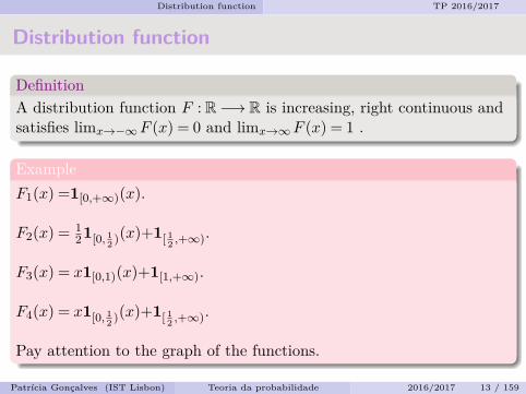
DefinitionA distribution function F : R−→ R is increasing, right continuous andsatisfies limx→−∞F (x) = 0 and limx→∞F (x) = 1 .
ExampleF1(x) =1[0,+∞)(x).
F2(x) = 121[0, 12 )(x)+1[ 1
2 ,+∞).
F3(x) = x1[0,1)(x)+1[1,+∞).
F4(x) = x1[0, 12 )(x)+1[ 12 ,+∞).
Pay attention to the graph of the functions.
Patrıcia Goncalves (IST Lisbon) Teoria da probabilidade 2016/2017 13 / 159
Distribution function TP 2016/2017
Distribution function and probability measure
LemmaEach probability measure µ in B defines a distribution function Fthrough the following correspondence: ∀x ∈ R,µ((−∞,x]) = F (x).(∗)
Exercise: do the proof of the lemma.
RemarkAs a consequence we have for −∞< a < b <∞ that
µ((a,b]) = F (b)−F (a); µ([a,b)) = F (b−)−F (a−);µ((a,b)) = F (b−)−F (a); µ([a,b]) = F (b)−F (a−);
For a dense subset D of R the correspondence above in (∗) isdetermined for x ∈D or if in the previous equalities we take a,b ∈D.
Patrıcia Goncalves (IST Lisbon) Teoria da probabilidade 2016/2017 14 / 159
Distribution function TP 2016/2017
TheoremEach distribution function F determines a probability measure µ in Bthrough one of the correspondences given above.
The question now is: Is this probability measure µ unique?
TheoremLet µ and ν be two probability measures defined in the same σ-algebra Fgenerated by the algebra F0. If µ(E) = ν(E) for any E ∈ F0 then µ= ν.
Exercise: do the proof of the two theorems above.
Patrıcia Goncalves (IST Lisbon) Teoria da probabilidade 2016/2017 15 / 159
Distribution function TP 2016/2017
TheoremGiven a probability measure µ in B there exists a unique distributionfunction F which satisfies µ((−∞,x]) = F (x) ∀x ∈ R. Conversely,given a distribution function F , there exists a unique probabilitymeasure µ in B satisfying µ((−∞,x]) = F (x) ∀x ∈ R.
We shall call µ the probability measure of F and F the distributionfunction of µ.
Patrıcia Goncalves (IST Lisbon) Teoria da probabilidade 2016/2017 16 / 159
Distribution function TP 2016/2017
ExampleInstead of (R,B) we can consider a restriction to a fixed interval [a,b].As example take U = [0,1]. Let us see how to define F .
Let F be a distribution function such that F (x) = 0, if x < 0 andF (x) = 1, if x≥ 1.
The probability measure µ will have support [0,1] sinceµ(−∞,0) = 0 = µ(1,+∞).
The trace of (R,B,µ) in U can be denoted by (U ,Bu,m), where Bu isthe trace of B in U and any probability measure in Bu can be seen asthat trace.
As example, we have the uniform distribution given for F3(·) above.
Patrıcia Goncalves (IST Lisbon) Teoria da probabilidade 2016/2017 17 / 159
Distribution function TP 2016/2017
Atoms
DefinitionAn atom of a measure µ defined in B is a singleton x such thatµ(x)> 0.
DefinitionA measure is said to be atomic if and only if µ is zero on any set notcontaining any atom.
Prove that if F is the distribution function of µ then
µ(x) = F (x)−F (x−).
Prove that µ is atomless (that is µ does not have atoms) if andonly if F is continuous.
Patrıcia Goncalves (IST Lisbon) Teoria da probabilidade 2016/2017 18 / 159
Distribution function TP 2016/2017
Monotone functionsLet f be an increasing function defined on R. This means that for allx≤ y it holds f(x)≤ f(y). Let us see some properties of these kind offunctions.
1 Both lateral limits exist and are finite for any x ∈ R:
limy↓x
f(y) = f(x+) and limy↑x
f(y) = f(x−).
2 When x=±∞ the limits above exist but can be equal to ±∞.3 The function is continuous (resp. right-continuous) at x if and
only if the limits above are both (resp. f(x+) is) equal to f(x).4 We say that the function has a jump at x if the limits above exist
but are different. The value f(x) has to satisfy
f(x−)≤ f(x)≤ f(x+.)5 When there is a jump at x, we say that x is a point of jump of f
and f(x+)−f(x−) is the size of the jump.Patrıcia Goncalves (IST Lisbon) Teoria da probabilidade 2016/2017 19 / 159
Distribution function TP 2016/2017
The set of jumps of f is countable (can be finite.)
To prove this, first associate to each point of jump x, the intervalIx = (f(x−),f(x+)). Then, if x′ is another point of jump of f andx < x′, then there exists x such that x < x < x′ and
f(x+)≤ f(x)≤ f(x′−).
As a consequence the intervals Ix and Ix′ are disjoint and can beconsecutive if f(x+) = f(x′−). Therefore we associate to the set ofpoints of jump of f a collection of disjoint intervals in the range of f .Now, this collection is, at most, countable since each interval contains arational number, so that the collection of intervals is in one-to-onecorrespondence with a certain subset of the rational numbers, beingthe latter countable.Since the set of points of jump of f is in one-to-one correspondencewith the set of intervals associated with it, then the proof ends.
Patrıcia Goncalves (IST Lisbon) Teoria da probabilidade 2016/2017 20 / 159
Distribution function TP 2016/2017
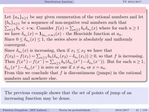
ExampleLet ann≥1 be any given enumeration of the rational numbers and letbnn≥1 be a sequence of non-negative real numbers such that∑n≥1 bn <+∞. Consider f(x) =
∑n≥1 bnδan(x) where for each n≥ 1
we have δan(x) = 1[an,+∞)(x) - the Heaviside function at an.Since 0≤ δan(x)≤ 1, the series above is absolutely and uniformlyconvergent.Since δan(x) is increasing, then if x1 ≤ x2 we have thatf(x2)−f(x1) =
∑n≥1 bn(δan(x2)− δan(x1))≥ 0, so that f is increasing.
Then f(x+)−f(x−) =∑n≥1 bn(δan(x+)− δan(x−)). But for each n≥ 1,
δan(x+)− δan(x−) is zero or one if x 6= an or x= an.From this we conclude that f is discontinuous (jumps) in the rationalnumbers and nowhere else.
The previous example shows that the set of points of jump of anincreasing function may be dense.
Patrıcia Goncalves (IST Lisbon) Teoria da probabilidade 2016/2017 21 / 159

Random variables TP 2016/2017
Random variables
Patrıcia Goncalves (IST Lisbon) Teoria da probabilidade 2016/2017 22 / 159
Random variables TP 2016/2017
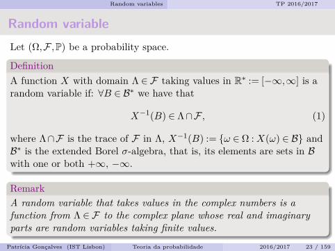
Random variableLet (Ω,F ,P) be a probability space.
DefinitionA function X with domain Λ ∈ F taking values in R∗ := [−∞,∞] is arandom variable if: ∀B ∈ B∗ we have that
X−1(B) ∈ Λ∩F , (1)
where Λ∩F is the trace of F in Λ, X−1(B) := ω ∈ Ω :X(ω) ∈ B andB∗ is the extended Borel σ-algebra, that is, its elements are sets in Bwith one or both +∞, −∞.
RemarkA random variable that takes values in the complex numbers is afunction from Λ ∈ F to the complex plane whose real and imaginaryparts are random variables taking finite values.
Patrıcia Goncalves (IST Lisbon) Teoria da probabilidade 2016/2017 23 / 159
Random variables TP 2016/2017
Random variable
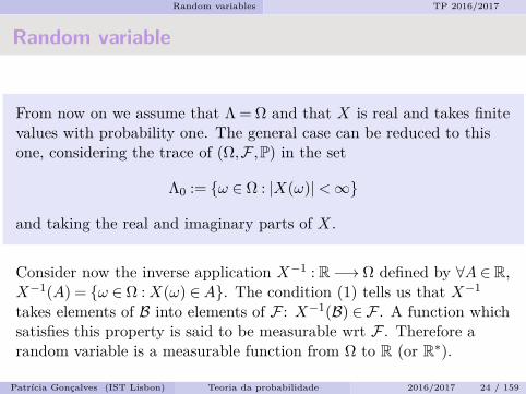
From now on we assume that Λ = Ω and that X is real and takes finitevalues with probability one. The general case can be reduced to thisone, considering the trace of (Ω,F ,P) in the set
Λ0 := ω ∈ Ω : |X(ω)|<∞
and taking the real and imaginary parts of X.
Consider now the inverse application X−1 : R−→ Ω defined by ∀A ∈ R,X−1(A) = ω ∈ Ω :X(ω) ∈A. The condition (1) tells us that X−1
takes elements of B into elements of F : X−1(B) ∈ F . A function whichsatisfies this property is said to be measurable wrt F . Therefore arandom variable is a measurable function from Ω to R (or R∗).
Patrıcia Goncalves (IST Lisbon) Teoria da probabilidade 2016/2017 24 / 159
Random variables TP 2016/2017
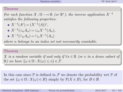
TheoremFor each function X : Ω−→ R (or R∗), the inverse application X−1
satisfies the following properties:X−1(Ac) = (X−1(A))c,X−1(∪αAα) = ∪αX−1(Aα),X−1(∩αAα) = ∩αX−1(Aα)
where α belongs to an index set not necessarily countable.
TheoremX is a random variable if and only if ∀x ∈ R (or x in a dense subset ofR) we have ω ∈ Ω :X(ω)≤ x ∈ F .
In this case since P is defined in F we denote the probability wrt P ofthe set ω ∈ Ω :X(ω) ∈B simply by P(X ∈B), for B ∈ B.
Patrıcia Goncalves (IST Lisbon) Teoria da probabilidade 2016/2017 25 / 159
Random variables TP 2016/2017
TheoremEach random variable X defined on a probability space (Ω,F ,P)induces a probability space (R,B,µ) through the followingcorrespondence ∀B ∈ B µ(B) = P(X−1(B)) = P(X ∈B).
Remark1. The collection of sets X−1(S) ; S ∈ R is a σ-algebra for anyfunction X.
2. In case X is a random variable, the collection X−1(B) ;B ∈ B isthe σ-algebra generated by X, which consists in the smallest subσ-algebra of F which contains all the sets of the formω ∈ Ω :X(ω)≤ x with x ∈ R.
3. The measure µ is going to be denoted by µ := PoX−1 and it is calledthe probability distribution measure of X and its associated F is thedistribution function of X: F (x) = µ((−∞,x]) = P(X ≤ x).
Patrıcia Goncalves (IST Lisbon) Teoria da probabilidade 2016/2017 26 / 159
Random variables TP 2016/2017
Identically distributed random variablesNote that X determines µ and µ determines F , the converse is false.Two random variables which have the same distribution are said to beidentically distributed.ExampleConsider the probability space (U ,B,m), U = [0,1], B is the Borelσ-algebra in U and m is the Lebesgue measure; and the randomvariables Xi : U −→ U given by X1(ω) = ω and X2(ω) = 1−ω.We observe that X1 6=X2 but they are identically distributed:m(ω ∈ U :X1(ω)≤ x) =m(ω ∈ U : ω ≤ x) =m([0,x]) = x andm(ω ∈ U :X2(ω)≤ x) =m(ω ∈ U : 1−ω ≤ x) =m(ω ∈ U : 1−x≤ ω) =1−m(ω < 1−x) = 1−m([0,1−x]) = 1− (1−x) = x.
Theorem (Constructing random variables)If X is a random variable and f : R−→ R is a Borel measurablefunction (that is f−1(B) ∈ B), then f(X) is a random variable.
Patrıcia Goncalves (IST Lisbon) Teoria da probabilidade 2016/2017 27 / 159

Distribution functions TP 2016/2017
Distribution functions
Patrıcia Goncalves (IST Lisbon) Teoria da probabilidade 2016/2017 28 / 159
Distribution functions TP 2016/2017
Distribution functionsRecall the definition of a distribution function. Let ajj≥1 be thecountable set of points of jump of F and let bj be the size of the jumpat aj : F (a+
j )−F (a−j ) = F (aj)−F (a−j ) = bj . Let
Fd(x) =∑j≥1
bjδaj (x),
where δaj (x) is the Heaviside function at aj . The function Fdrepresents all the jumps of F in (−∞,x]. Note that Fd is increasing,right-continuous, Fd(−∞) = 0 and Fd(+∞) =
∑j≥1 bj ≤ 1. The
function Fd is the jumping part of F .Theorem
The function Fc(x) = F (x)−Fd(x) is positive, increasing, continuous.
Exercise: do the proof of the theorem.Patrıcia Goncalves (IST Lisbon) Teoria da probabilidade 2016/2017 29 / 159
Distribution functions TP 2016/2017
TheoremLet F be a distribution function. Suppose that there exists a continuousfunction Gc and a function Gd of the form Gd(x) =
∑j≥1 b
′jδa′j (x),
where a′jj≥1 is a countable set of real numbers and∑j≥1 b
′j <∞,
such that F =Gc+Gd. Then Gc = Fc and Gd = Fd where Fc and Fdwere defined above.
Exercise: do the proof of the theorem.
DefinitionA distribution function that can be represented in the formF =
∑j≥1 bjδaj , where ajj≥1 is a countable (or finite) set of real
numbers bj > 0 for every j and∑j≥1 bj = 1 is called a discrete
distribution function. A distribution function that is continuouseverywhere is called a continuous distribution function.
Patrıcia Goncalves (IST Lisbon) Teoria da probabilidade 2016/2017 30 / 159
Distribution functions TP 2016/2017
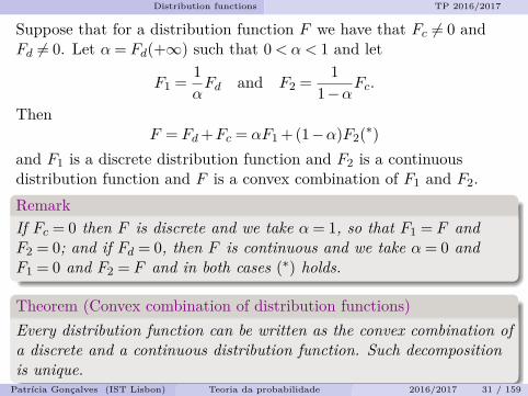
Suppose that for a distribution function F we have that Fc 6= 0 andFd 6= 0. Let α= Fd(+∞) such that 0< α < 1 and let
F1 = 1αFd and F2 = 1
1−αFc.
ThenF = Fd+Fc = αF1 + (1−α)F2(∗)
and F1 is a discrete distribution function and F2 is a continuousdistribution function and F is a convex combination of F1 and F2.RemarkIf Fc = 0 then F is discrete and we take α= 1, so that F1 = F andF2 = 0; and if Fd = 0, then F is continuous and we take α= 0 andF1 = 0 and F2 = F and in both cases (∗) holds.
Theorem (Convex combination of distribution functions)Every distribution function can be written as the convex combination ofa discrete and a continuous distribution function. Such decompositionis unique.
Patrıcia Goncalves (IST Lisbon) Teoria da probabilidade 2016/2017 31 / 159
Distribution functions TP 2016/2017
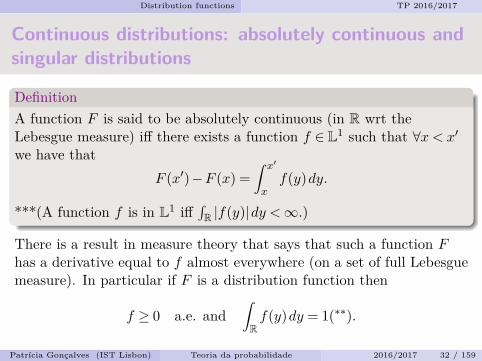
Continuous distributions: absolutely continuous andsingular distributions
DefinitionA function F is said to be absolutely continuous (in R wrt theLebesgue measure) iff there exists a function f ∈ L1 such that ∀x < x′
we have thatF (x′)−F (x) =
∫ x′
xf(y)dy.
***(A function f is in L1 iff∫R |f(y)|dy <∞.)
There is a result in measure theory that says that such a function Fhas a derivative equal to f almost everywhere (on a set of full Lebesguemeasure). In particular if F is a distribution function then
f ≥ 0 a.e. and∫Rf(y)dy = 1(∗∗).
Patrıcia Goncalves (IST Lisbon) Teoria da probabilidade 2016/2017 32 / 159
Distribution functions TP 2016/2017
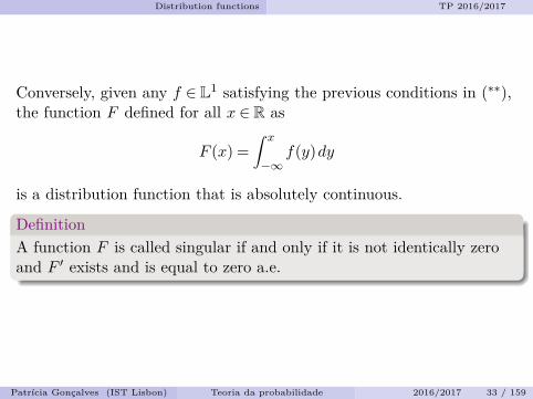
Conversely, given any f ∈ L1 satisfying the previous conditions in (∗∗),the function F defined for all x ∈ R as
F (x) =∫ x
−∞f(y)dy
is a distribution function that is absolutely continuous.
DefinitionA function F is called singular if and only if it is not identically zeroand F ′ exists and is equal to zero a.e.
Patrıcia Goncalves (IST Lisbon) Teoria da probabilidade 2016/2017 33 / 159
Distribution functions TP 2016/2017
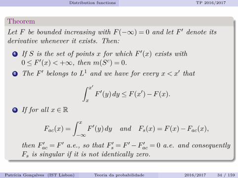
TheoremLet F be bounded increasing with F (−∞) = 0 and let F ′ denote itsderivative whenever it exists. Then:
1 If S is the set of points x for which F ′(x) exists with0≤ F ′(x)<+∞, then m(Sc) = 0.
2 The F ′ belongs to L1 and we have for every x < x′ that∫ x′
xF ′(y)dy ≤ F (x′)−F (x).
3 If for all x ∈ R
Fac(x) =∫ x
−∞F ′(y)dy and Fs(x) = F (x)−Fac(x),
then F ′ac = F ′ a.e., so that F ′s = F ′−F ′ac = 0 a.e. and consequentlyFs is singular if it is not identically zero.
Patrıcia Goncalves (IST Lisbon) Teoria da probabilidade 2016/2017 34 / 159
Distribution functions TP 2016/2017
DefinitionAny positive function f that is equal to F ′ a.e. is called a density of F .Fac is the absolutely continuous part of F and Fs is its singular part.
RemarkNote that:1. the discrete part Fd defined above is part of the singular part Fsdefined above;2. Fac is increasing and that Fac ≤ F . (Check it!)Moreover, if x < x′ then Fs(x′)−Fs(x) = F (x′)−F (x)−
∫ x′x f(y)dy ≥ 0,
(from (2) of the previous theorem) therefore Fs is also increasing andFs ≤ F . (Check it!)
TheoremEvery distribution function F can be written as the convex combinationof a discrete, a singular and an absolutely continuous distributionsfunction and such decomposition is unique.
Patrıcia Goncalves (IST Lisbon) Teoria da probabilidade 2016/2017 35 / 159
Distribution functions TP 2016/2017
Continuous distribution function: the singular case
Let us construct the Cantor set. From the closed interval [0,1] removethe central interval (1
3 ,23). Then in the two remaining intervals remove
the central intervals (19 ,
29) and (7
9 ,89). After the 1st step we remain
with two intervals of size 13 . In the 2nd step we remain with four
intervals of size 132 and so on. After n steps we have removed
1+2+4+8+ · · ·+2n−1 = 2n−1 disjoint intervals and remain 2n closedintervals of size 1
3n . Let us order these intervals, by order from left toright and denote them by Jn,k, where 1≤ k ≤ 2n−1 and denote theirunion by Un. Note that
m(Un) = 1−(2
3)n.
As n increases the set Un increases to an open set U and let C := U c
(the complementary wrt [0,1]) be the Cantor set. Thenm(C) = 1−m(U) = 1− limn→∞m(Un) = 1−1 = 0.
Patrıcia Goncalves (IST Lisbon) Teoria da probabilidade 2016/2017 36 / 159
Distribution functions TP 2016/2017
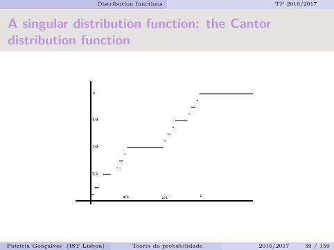
The Cantor distribution function
Now we define the Cantor distribution function. For each n,k, withn≥ 1 and k = 1, · · · ,2n−1 let cn,k = k
2n and let us define F in U in thefollowing way:
if x ∈ Jn,k then F (x) = cn,k.
In each Jn,k the function F is constant and it is strictly greater on anyJn,k′ at the right of Jn,k. Therefore, F is increasing and F (0+) = 0 andF (1−) = 1.Now we complete the definition by setting F (x) = 0 for x≤ 0 andF (x) = 1 for x≥ 1.
⇒ Up to here the function F is defined on the domainD = (−∞,0]∪U ∪ [1,+∞) and is increasing.
Patrıcia Goncalves (IST Lisbon) Teoria da probabilidade 2016/2017 37 / 159
Distribution functions TP 2016/2017
Now, since each Jn,k is at a distance which is greater or equal than1/3n from any other Jn,k′ and since the total variation of F over eachof the 2n disjoint intervals that remain after removing Jn,k is 1
2n , itfollows that
0≤ x′−x≤ 13n ⇒ 0≤ F (x′)−F (x)≤ 1
2nThen, the function F is uniformly continuous on D. (D is dense in R).By a result (*) there exists a continuous and increasing function Fdefined on R that coincides with F on D.This function F is a continuous distribution function that is constanton each Jn,k so that F ′ = 0 on U and also on R\C, which means that Fis singular.
(*) Let f be increasing on a dense subset D of R. If for any x ∈ Rf(x) = infx<t∈D f(t), then f is increasing and right continuouseverywhere. If f uniformly continuous, then f is uniformly continuous.
Patrıcia Goncalves (IST Lisbon) Teoria da probabilidade 2016/2017 38 / 159
Distribution functions TP 2016/2017
A singular distribution function: the Cantordistribution function
Patrıcia Goncalves (IST Lisbon) Teoria da probabilidade 2016/2017 39 / 159
Distribution functions TP 2016/2017
Random variables
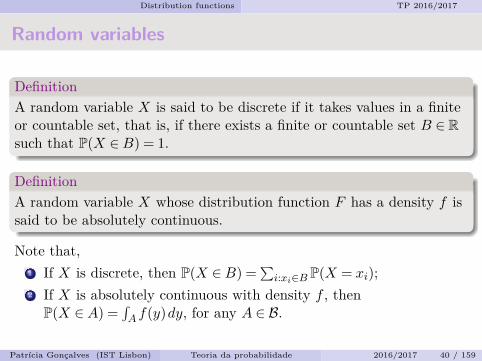
DefinitionA random variable X is said to be discrete if it takes values in a finiteor countable set, that is, if there exists a finite or countable set B ∈ Rsuch that P(X ∈B) = 1.
DefinitionA random variable X whose distribution function F has a density f issaid to be absolutely continuous.
Note that,1 If X is discrete, then P(X ∈B) =
∑i:xi∈B P(X = xi);
2 If X is absolutely continuous with density f , thenP(X ∈A) =
∫A f(y)dy, for any A ∈ B.
Patrıcia Goncalves (IST Lisbon) Teoria da probabilidade 2016/2017 40 / 159
Distribution functions TP 2016/2017
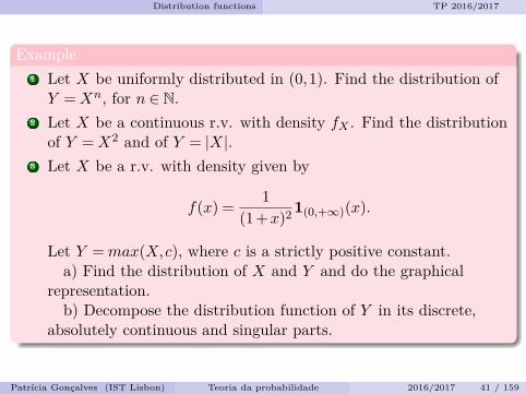
Example1 Let X be uniformly distributed in (0,1). Find the distribution ofY =Xn, for n ∈ N.
2 Let X be a continuous r.v. with density fX . Find the distributionof Y =X2 and of Y = |X|.
3 Let X be a r.v. with density given by
f(x) = 1(1 +x)2 1(0,+∞)(x).
Let Y =max(X,c), where c is a strictly positive constant.a) Find the distribution of X and Y and do the graphical
representation.b) Decompose the distribution function of Y in its discrete,
absolutely continuous and singular parts.
Patrıcia Goncalves (IST Lisbon) Teoria da probabilidade 2016/2017 41 / 159

Random vectors TP 2016/2017
Random vectors
Patrıcia Goncalves (IST Lisbon) Teoria da probabilidade 2016/2017 42 / 159
Random vectors TP 2016/2017
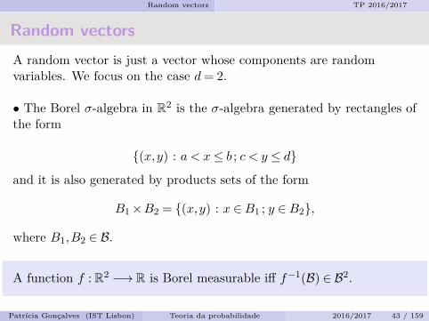
Random vectorsA random vector is just a vector whose components are randomvariables. We focus on the case d= 2.
• The Borel σ-algebra in R2 is the σ-algebra generated by rectangles ofthe form
(x,y) : a < x≤ b ; c < y ≤ d
and it is also generated by products sets of the form
B1×B2 = (x,y) : x ∈B1 ; y ∈B2,
where B1,B2 ∈ B.
A function f : R2 −→ R is Borel measurable iff f−1(B) ∈ B2.
Patrıcia Goncalves (IST Lisbon) Teoria da probabilidade 2016/2017 43 / 159
Random vectors TP 2016/2017
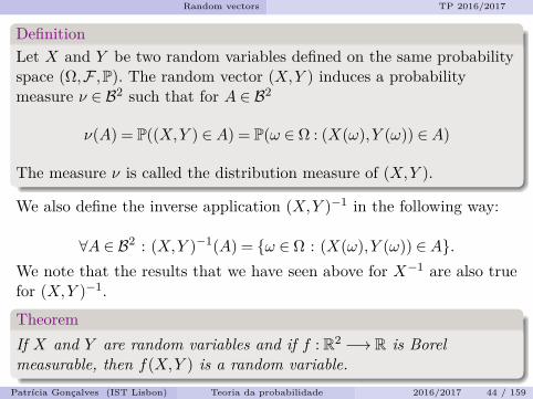
DefinitionLet X and Y be two random variables defined on the same probabilityspace (Ω,F ,P). The random vector (X,Y ) induces a probabilitymeasure ν ∈ B2 such that for A ∈ B2
ν(A) = P((X,Y ) ∈A) = P(ω ∈ Ω : (X(ω),Y (ω)) ∈A)
The measure ν is called the distribution measure of (X,Y ).
We also define the inverse application (X,Y )−1 in the following way:
∀A ∈ B2 : (X,Y )−1(A) = ω ∈ Ω : (X(ω),Y (ω)) ∈A.We note that the results that we have seen above for X−1 are also truefor (X,Y )−1.
TheoremIf X and Y are random variables and if f : R2 −→ R is Borelmeasurable, then f(X,Y ) is a random variable.
Patrıcia Goncalves (IST Lisbon) Teoria da probabilidade 2016/2017 44 / 159
Random vectors TP 2016/2017
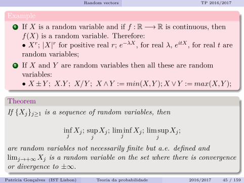
Example1 If X is a random variable and if f : R−→ R is continuous, thenf(X) is a random variable. Therefore:• Xr; |X|r for positive real r; e−λX , for real λ, eitX , for real t arerandom variables;
2 If X and Y are random variables then all these are randomvariables:• X±Y ; X.Y ; X/Y ; X ∧Y :=min(X,Y );X ∨Y :=max(X,Y );
TheoremIf Xjj≥1 is a sequence of random variables, then
infjXj ; sup
jXj ; liminf
jXj ; limsup
jXj ;
are random variables not necessarily finite but a.e. defined andlimj→+∞Xj is a random variable on the set where there is convergenceor divergence to ±∞.
Patrıcia Goncalves (IST Lisbon) Teoria da probabilidade 2016/2017 45 / 159
Random vectors TP 2016/2017
The distribution function of a random vector
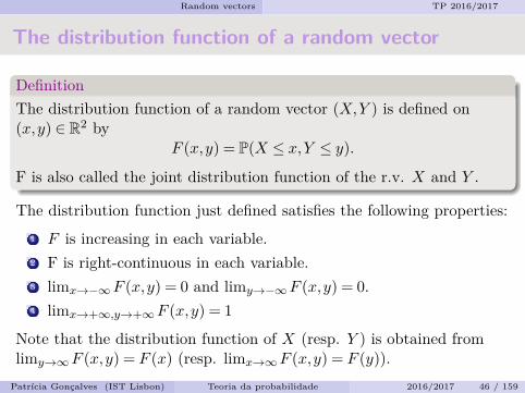
DefinitionThe distribution function of a random vector (X,Y ) is defined on(x,y) ∈ R2 by
F (x,y) = P(X ≤ x,Y ≤ y).
F is also called the joint distribution function of the r.v. X and Y .
The distribution function just defined satisfies the following properties:1 F is increasing in each variable.2 F is right-continuous in each variable.3 limx→−∞F (x,y) = 0 and limy→−∞F (x,y) = 0.4 limx→+∞,y→+∞F (x,y) = 1
Note that the distribution function of X (resp. Y ) is obtained fromlimy→∞F (x,y) = F (x) (resp. limx→∞F (x,y) = F (y)).
Patrıcia Goncalves (IST Lisbon) Teoria da probabilidade 2016/2017 46 / 159

Random vectors TP 2016/2017
The distribution function of a random vector
The properties above are not sufficient to guarantee that a functionF : R2→ R2 is the distribution function of a random vector. Let us seean example.
Example ( Let F (x,y) = 1x≥0,y≥0,x+y≥1. )It is easy to see that F satisfies the properties above, nevertheless it isnot the distribution function of a random vector. Suppose it is. Thenwe would have, for example, that: P(X ∈ (0,1],Y ∈ (0,1]) =−1, whichcannot happen since P is a probability.
We need to introduce some extra condition, in order to avoid theprevious example, which is the following:• For any a1 < b1 and a2 < b2 we have P(X ∈ (a1, b1],Y ∈ (a2, b2])≥ 0.A function F satisfying the properties above is the distributionfunction of a random vector.
Patrıcia Goncalves (IST Lisbon) Teoria da probabilidade 2016/2017 47 / 159
Random vectors TP 2016/2017
Exercises
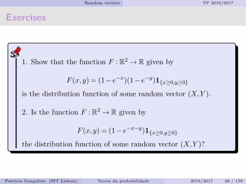
1. Show that the function F : R2→ R given by
F (x,y) = (1−e−x)(1−e−y)1x≥0,y≥0
is the distribution function of some random vector (X,Y ).
2. Is the function F : R2→ R given by
F (x,y) = (1−e−x−y)1x≥0,y≥0
the distribution function of some random vector (X,Y )?
Patrıcia Goncalves (IST Lisbon) Teoria da probabilidade 2016/2017 48 / 159
Random vectors TP 2016/2017
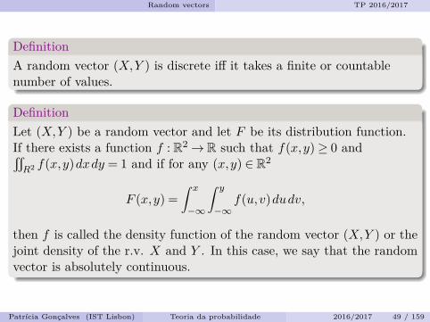
DefinitionA random vector (X,Y ) is discrete iff it takes a finite or countablenumber of values.
DefinitionLet (X,Y ) be a random vector and let F be its distribution function.If there exists a function f : R2→ R such that f(x,y)≥ 0 andsR2 f(x,y)dxdy = 1 and if for any (x,y) ∈ R2
F (x,y) =∫ x
−∞
∫ y
−∞f(u,v)dudv,
then f is called the density function of the random vector (X,Y ) or thejoint density of the r.v. X and Y . In this case, we say that the randomvector is absolutely continuous.
Patrıcia Goncalves (IST Lisbon) Teoria da probabilidade 2016/2017 49 / 159

Stochastic Independence TP 2016/2017
Stochastic Independence
Patrıcia Goncalves (IST Lisbon) Teoria da probabilidade 2016/2017 50 / 159
Stochastic Independence TP 2016/2017
Independence
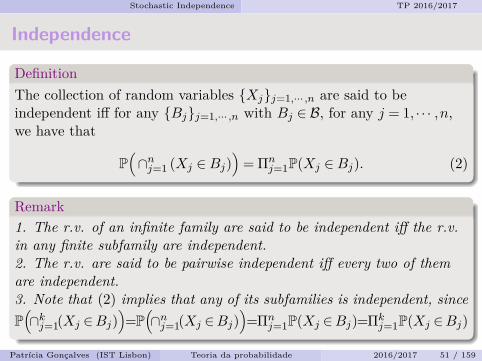
DefinitionThe collection of random variables Xjj=1,··· ,n are said to beindependent iff for any Bjj=1,··· ,n with Bj ∈ B, for any j = 1, · · · ,n,we have that
P(∩nj=1 (Xj ∈Bj)
)= Πn
j=1P(Xj ∈Bj). (2)
Remark1. The r.v. of an infinite family are said to be independent iff the r.v.in any finite subfamily are independent.2. The r.v. are said to be pairwise independent iff every two of themare independent.3. Note that (2) implies that any of its subfamilies is independent, sinceP(∩kj=1(Xj ∈Bj)
)=P(∩nj=1(Xj ∈Bj)
)=Πn
j=1P(Xj ∈Bj)=Πkj=1P(Xj ∈Bj)
Patrıcia Goncalves (IST Lisbon) Teoria da probabilidade 2016/2017 51 / 159
Stochastic Independence TP 2016/2017
Remark
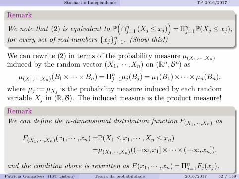
We note that (2) is equivalent to P(∩nj=1 (Xj ≤ xj)
)= Πn
j=1P(Xj ≤ xj),for every set of real numbers xjnj=1. (Show this!)
We can rewrite (2) in terms of the probability measure µ(X1,··· ,Xn)induced by the random vector (X1, · · · ,Xn) on (Rn,Bn) as
µ(X1,··· ,Xn)(B1×·· ·×Bn) = Πnj=1µj(Bj) = µ1(B1)×·· ·×µn(Bn),
where µj := µXj is the probability measure induced by each randomvariable Xj in (R,B). The induced measure is the product measure!
RemarkWe can define the n-dimensional distribution function F(X1,··· ,Xn) as
F(X1,··· ,Xn)(x1, · · · ,xn) =P(X1 ≤ x1, · · · ,Xn ≤ xn)=µ(X1,··· ,Xn)((−∞,x1]×·· ·× (−∞,xn]).
and the condition above is rewritten as F (x1, · · · ,xn) = Πnj=1Fj(xj).
Patrıcia Goncalves (IST Lisbon) Teoria da probabilidade 2016/2017 52 / 159
Stochastic Independence TP 2016/2017
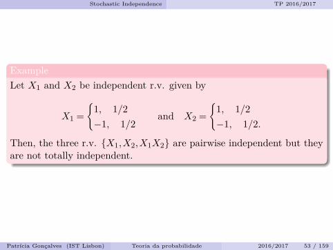
ExampleLet X1 and X2 be independent r.v. given by
X1 =
1, 1/2−1, 1/2
and X2 =
1, 1/2−1, 1/2.
Then, the three r.v. X1,X2,X1X2 are pairwise independent but theyare not totally independent.
Patrıcia Goncalves (IST Lisbon) Teoria da probabilidade 2016/2017 53 / 159
Stochastic Independence TP 2016/2017
Independent eventsWhenever a probability space (Ω,F ,P) is fixed, the sets in F will becalled events. We have seen above the notion of independent r.v. butwhat about independent events?DefinitionWe say that the events Ejnj=1 are independent iff their indicators areindependent, that is, for any subset j1, · · · , j` of 1, · · · ,n we havethat P
(∩`k=1Ejk
)= Π`
k=1P(Ejk).
TheoremIf Xjnj=1 are independent r.v. and fjnj=1 are Borel measurablefunctions, then fj(Xj)nj=1 are independent r.v.
Do the proof of the theorem.
Patrıcia Goncalves (IST Lisbon) Teoria da probabilidade 2016/2017 54 / 159
Stochastic Independence TP 2016/2017
We have seen above that if X1, · · · ,Xn are independent r.v. thenF(X1,··· ,Xn)(x1, · · · ,xn) = Πn
j=1FXj (xj). Now let us see the reciprocal.
PropositionIf there exist functions F1, · · · ,Fn such that
limxj→∞
Fj(xj) = 1
for all j = 1, · · · ,n and if for all (x1, · · · ,xn) ∈ Rn
F(X1,··· ,Xn)(x1, · · · ,xn) = Πnj=1Fj(xj),
then Xjnj=1 are independent and Fj := FXj for all j = 1, · · · ,n.
Do the proof of the proposition.
Patrıcia Goncalves (IST Lisbon) Teoria da probabilidade 2016/2017 55 / 159
Stochastic Independence TP 2016/2017
Criterion for independence
PropositionIf Xjnj=1 are independent r.v. with densities fX1 , · · · ,fXn, thenthe function
f(x1, · · · ,xn) = Πnj=1fXj (xj)
is the joint density of Xjnj=1 or the density of the random vector(X1, · · · ,Xn) .On the other hand, if X1, · · · ,Xn has a joint density f whichsatisfies
f(x1, · · · ,xn) = Πnj=1fj(xj)
for all (x1, · · · ,xn) ∈ Rn with fj(x)≥ 0 and∫R fj(x)dx= 1, then
X1, · · · ,Xn are independent and fj is the density of Xj.
Do the proof of the theorem.Patrıcia Goncalves (IST Lisbon) Teoria da probabilidade 2016/2017 56 / 159
Stochastic Independence TP 2016/2017
Constructing two independent random variables I
Let (Ω1,F1,P1) and (Ω2,F2,P2) where (Fj is the total σ-algebra) bediscrete probability spaces.We define the product space Ω2 := Ω1×Ω2 as the space of pointsω = (ω1,ω2) with ω1 ∈ Ω1 and ω2 ∈ Ω2. The product σ-algebra F2 isthe collection of all the subsets of Ω2. We know from the beginning ofthe course that the probability measures P1 and P2 are determined bytheir values in ω1, ω2 respectively. Since Ω2 is also countable we candefine a probability measure P2 in F2 as
P2((ω1,ω2)) = P1(ω1)P2(ω2)
which is the product measure of P1 and P2. Check that it is aprobability measure. It has the property that if S1 ∈ F1 and S2 ∈ F2,then
P2(S1×S2) = P1(S1)P2(S2).
Patrıcia Goncalves (IST Lisbon) Teoria da probabilidade 2016/2017 57 / 159
Stochastic Independence TP 2016/2017
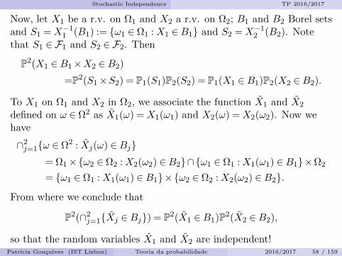
Now, let X1 be a r.v. on Ω1 and X2 a r.v. on Ω2; B1 and B2 Borel setsand S1 =X−1
1 (B1) := ω1 ∈ Ω1 :X1 ∈B1 and S2 =X−12 (B2). Note
that S1 ∈ F1 and S2 ∈ F2. Then
P2(X1 ∈B1×X2 ∈B2)=P2(S1×S2) = P1(S1)P2(S2) = P1(X1 ∈B1)P2(X2 ∈B2).
To X1 on Ω1 and X2 in Ω2, we associate the function X1 and X2defined on ω ∈ Ω2 as X1(ω) =X1(ω1) and X2(ω) =X2(ω2). Now wehave∩2j=1ω ∈ Ω2 : Xj(ω) ∈Bj
= Ω1×ω2 ∈ Ω2 :X2(ω2) ∈B2∩ω1 ∈ Ω1 :X1(ω1) ∈B1×Ω2
= ω1 ∈ Ω1 :X1(ω1) ∈B1×ω2 ∈ Ω2 :X2(ω2) ∈B2.
From where we conclude that
P2(∩2j=1Xj ∈Bj) = P2(X1 ∈B1)P2(X2 ∈B2),
so that the random variables X1 and X2 are independent!Patrıcia Goncalves (IST Lisbon) Teoria da probabilidade 2016/2017 58 / 159
Stochastic Independence TP 2016/2017
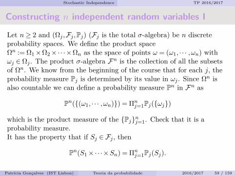
Constructing n independent random variables I
Let n≥ 2 and (Ωj ,Fj ,Pj) (Fj is the total σ-algebra) be n discreteprobability spaces. We define the product spaceΩn := Ω1×Ω2×·· ·×Ωn as the space of points ω = (ω1, · · · ,ωn) withωj ∈ Ωj . The product σ-algebra Fn is the collection of all the subsetsof Ωn. We know from the beginning of the course that for each j, theprobability measure Pj is determined by its value in ωj . Since Ωn isalso countable we can define a probability measure Pn in Fn as
Pn((ω1, · · · ,ωn)) = Πnj=1Pj(ωj)
which is the product measure of the Pjnj=1. Check that it is aprobability measure.It has the property that if Sj ∈ Fj , then
Pn(S1×·· ·×Sn) = Πnj=1Pj(Sj).
Patrıcia Goncalves (IST Lisbon) Teoria da probabilidade 2016/2017 59 / 159
Stochastic Independence TP 2016/2017
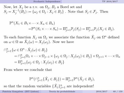
Now, let Xj be a r.v. on Ωj , Bj a Borel set andSj =X−1
j (Bj) := ωj ∈ Ωj :Xj ∈Bj . Note that Sj ∈ Fj . Then
Pn(X1 ∈B1×·· ·×Xn ∈Bn)=Pn(S1×·· ·×Sn) = Πn
j=1Pj(Sj) = Πnj=1Pj(Xj ∈Bj).
To each function Xj on Ωj we associate the function Xj on Ωn definedon ω ∈ Ω as Xj(ω) =Xj(ωj). Now we have
∩nj=1ω ∈ Ωn : Xj(ω) ∈Bj= ∩nj=1Ω1×·· ·×Ωj−1×ωj ∈ Ωj :Xj(ωj) ∈Bj×Ωj+1×·· ·×Ωn
= Πnj=1ωj ∈ Ωj :Xj(ωj) ∈Bj
From where we conclude that
Pn(∩nj=1Xj ∈Bj) = Πnj=1Pn(Xj ∈Bj),
so that the random variables Xjnj=1 are independent!Patrıcia Goncalves (IST Lisbon) Teoria da probabilidade 2016/2017 60 / 159
Stochastic Independence TP 2016/2017
Constructing independent random variables II
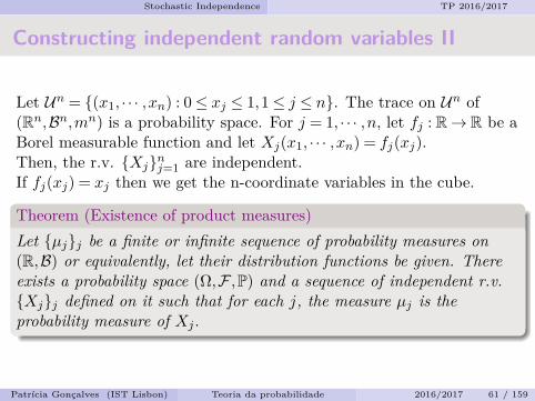
Let Un = (x1, · · · ,xn) : 0≤ xj ≤ 1,1≤ j ≤ n. The trace on Un of(Rn,Bn,mn) is a probability space. For j = 1, · · · ,n, let fj : R→ R be aBorel measurable function and let Xj(x1, · · · ,xn) = fj(xj).Then, the r.v. Xjnj=1 are independent.If fj(xj) = xj then we get the n-coordinate variables in the cube.
Theorem (Existence of product measures)Let µjj be a finite or infinite sequence of probability measures on(R,B) or equivalently, let their distribution functions be given. Thereexists a probability space (Ω,F ,P) and a sequence of independent r.v.Xjj defined on it such that for each j, the measure µj is theprobability measure of Xj .
Patrıcia Goncalves (IST Lisbon) Teoria da probabilidade 2016/2017 61 / 159
Stochastic Independence TP 2016/2017
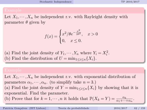
ExampleLet X1, · · · ,Xn be independent r.v. with Rayleight density withparameter θ given by
f(x) =
x2/θe−x22θ2 , x > 0
0, x≤ 0.
(a) Find the joint density of Y1, · · · ,Yn where Yi =X2i .
(b) Find the distribution of U = min1≤i≤nXi.
ExampleLet X1, · · · ,Xn be independent r.v. with exponential distribution ofparameters α1, · · · ,αn. (to simplify take n= 3.)(a) Find the joint density of Y = min1≤i≤nXi by showing that it isexponential. Find the parameter.(b) Prove that for k = 1, · · · ,n it holds that P(Xk = Y ) = αk
α1+···+αn .
Patrıcia Goncalves (IST Lisbon) Teoria da probabilidade 2016/2017 62 / 159

Mathematical Expectation TP 2016/2017
Mathematical Expectation
Patrıcia Goncalves (IST Lisbon) Teoria da probabilidade 2016/2017 63 / 159
Mathematical Expectation TP 2016/2017
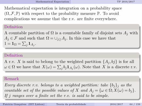
Mathematical expectation is integration on a probability space(Ω,F ,P) with respect to the probability measure P. To avoidcomplications we assume that the r.v. are finite everywhere.
DefinitionA countable partition of Ω is a countable family of disjoint sets Aj withAj ∈ F and such that Ω = ∪j≥Aj . In this case we have that1 = 1Ω =
∑j 1Aj .
DefinitionA r.v. X is said to belong to the weighted partition Aj , bj is for allω ∈ Ω we have that X(ω) =
∑j bj1Aj (ω). Note that X is a discrete r.v.
RemarkEvery discrete r.v. belongs to a weighted partition: take bjj as thecountable set of the possible values of X and Aj = ω ∈ Ω;X(ω) = bj.If j ranges over a finite set the r.v. is said to be simple.
Patrıcia Goncalves (IST Lisbon) Teoria da probabilidade 2016/2017 64 / 159
Mathematical Expectation TP 2016/2017
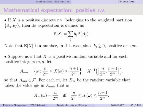
Mathematical expectation: positive r.v.• If X is a positive discrete r.v. belonging to the weighted partitionAj , bj, then its expectation is defined as
E[X] =∑j
bjP(Aj).
Note that E[X] is a number, in this case, since bj ≥ 0, positive or +∞.
• Suppose now that X is a positive random variable and for eachpositive integers m,n, let
Amn =ω : n
2m ≤X(ω)≤ n+ 12m
=X−1
([ n2m ,
n+ 12m
]),
so that Amn ∈ F . For each m, let Xm be the random variable thattakes the value n
2m in Amn, that is
Xm(ω) = n
2m iff n
2m ≤X(ω)≤ n+ 12m .
Patrıcia Goncalves (IST Lisbon) Teoria da probabilidade 2016/2017 65 / 159
Mathematical Expectation TP 2016/2017
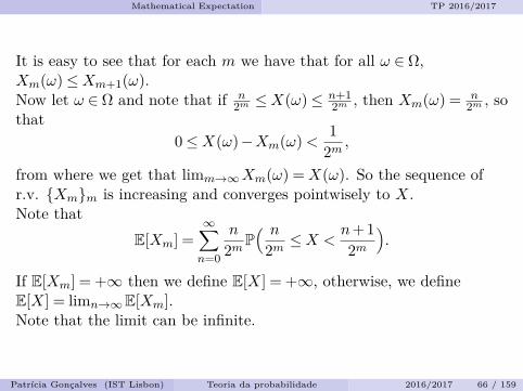
It is easy to see that for each m we have that for all ω ∈ Ω,Xm(ω)≤Xm+1(ω).Now let ω ∈ Ω and note that if n
2m ≤X(ω)≤ n+12m , then Xm(ω) = n
2m , sothat
0≤X(ω)−Xm(ω)< 12m ,
from where we get that limm→∞Xm(ω) =X(ω). So the sequence ofr.v. Xmm is increasing and converges pointwisely to X.Note that
E[Xm] =∞∑n=0
n
2mP( n
2m ≤X <n+ 12m
).
If E[Xm] = +∞ then we define E[X] = +∞, otherwise, we defineE[X] = limn→∞E[Xm].Note that the limit can be infinite.
Patrıcia Goncalves (IST Lisbon) Teoria da probabilidade 2016/2017 66 / 159
Mathematical Expectation TP 2016/2017
For a general X we take X =X+−X−, where X+ =X ∨0 andX− = (−X)∨0. Both X+,X− are positive, so their expectation isdefined and unless both expectations are +∞ we defineE[X] = E[X+]−E[X−]. We sat that X has finite or infinite expectationaccording to E[X] is finite or infinite.
When the expectation of X exists we use the notation
E[X] =∫
ΩX(ω)P(dω) =
∫ΩX(ω)dP.
For Λ ∈ F we have
E[X1Λ] =∫
ΛX(ω)P(dω) =
∫Ω
1Λ(ω)X(ω)dP
and it is called the integral of X wrt P over the set Λ.• When the integral above exists and is finite we say that X isintegrable in Λ wrt P.
Patrıcia Goncalves (IST Lisbon) Teoria da probabilidade 2016/2017 67 / 159
Mathematical Expectation TP 2016/2017
Example (Lebesgue-Stietjes integral)For (R,B,µ) and X = f and ω = x we have∫
ΛX(ω)P(dω) =
∫Λf(x)µ(dx) =
∫Λf(x)dµ.
When F is the distribution function of µ we also write (for Λ = (a,b])∫(a,b]
f(x)dF (x).
To distinguish the intervals (a,b], [a,b],(a,b) and [a,b) we use thenotation ∫ b+0
a+0,
∫ b+0
a−0,
∫ b−0
a+0,
∫ b−0
a−0.
For (U ,B,m) the integral is∫ ba f(x)m(dx) =
∫ ba f(x)dx. Since µ is atomless we do not need to
distinguish the intervals.Patrıcia Goncalves (IST Lisbon) Teoria da probabilidade 2016/2017 68 / 159
Mathematical Expectation TP 2016/2017
Properties of the mathematical expectation
In what follows X and Y are r.v. and a,b ∈ R and Λ ∈ F .
(1) Absolute integrability:∫
ΛXdP is finite iff∫
Λ |X|dP is finite.
(2) Linearity:∫
Λ(aX+ bY )dP = a∫
ΛXdP+ b∫
ΛY dP.
(3) Set additivity: If Λnn≥1 are disjoint, then∫∪n≥1Λn
XdP =∑n≥1
∫ΛnXdP.
(4) Positivity: If X ≥ 0 a.e. on Λ (this means there is a subset of Λwith weight one wrt P where X is positive), then∫
ΛXdP≥ 0.
Patrıcia Goncalves (IST Lisbon) Teoria da probabilidade 2016/2017 69 / 159
Mathematical Expectation TP 2016/2017
Properties of the mathematical expectation(5) Monotonicity: If X1 ≤X ≤X2 a.e. in Λ, then∫
ΛX1dP≤
∫ΛXdP≤
∫ΛX2dP.
(6) Mean value Theorem: If a≤X ≤ b a.e. in Λ, then
aP(Λ)≤∫
ΛXdP≤ bP(Λ).
(7) Modulus inequality:∣∣∣ ∫ΛXdP∣∣∣≤ ∫Λ |X|dP.
(8) Dominated convergence Theorem: If limn→∞Xn =X a.e. on Λ andif for n≥ 1 |Xn| ≤ Y a.e. on Λ and
∫ΛY dP<∞, then
limn→∞
∫ΛXndP =
∫ΛXdP =
∫Λ
limn→∞
XndP.
Patrıcia Goncalves (IST Lisbon) Teoria da probabilidade 2016/2017 70 / 159
Mathematical Expectation TP 2016/2017
Properties of the mathematical expectation(9) Bounded convergence Theorem: If limn→∞Xn =X a.e. on Λ andthere exists a constant M such that n≥ 1 |Xn| ≤M a.e. on Λ, then theprevious equality is true.
(10) Monotone convergence Theorem: If Xn ≥ 0 and Xn ↑X a.e. on Λ,then the previous equality is true if we allow +∞ as a value.
(11) Integration term by term: If∑n≥1
∫Λ |Xn|dP<∞, then∑
n≥1 |Xn|<∞ a.e. on Λ, so that∑n≥1Xn converges a.e. on Λ and∫
Λ
∑n≥1
XndP =∑n≥1
∫ΛXndP.
(12) Fatou’s Lemma: If Xn ≥ 0 a.e. on Λ, then∫Λ
(liminfn→∞
Xn)dP≤ liminfn→∞
∫ΛXndP.
Patrıcia Goncalves (IST Lisbon) Teoria da probabilidade 2016/2017 71 / 159
Mathematical Expectation TP 2016/2017
The Lebesgue-Stieltjes integralLet f be a continuous function defined on [a,b] and let F be adistribution function. The Riemann-Stieltjes integral of f on [a,b] wrtF is defined as the limit of the Riemann sums of the form
n∑i=1
f(xi)(F (xi+1)−F (xi)),
where x1 = a,xn = b, xi < xi+1 and xi is an arbitrary point in [xi,xi+1].The limit is takes by making the norm of the partition xii tending to0, that is maxi=1,··· ,n(xi+1−xi)→ 0. The limit exists, when f iscontinuous, and it is denoted by
∫ ba f(x)dF (x). Note that∫
Rf(x)dF (x) = lim
a→−∞,b→+∞
∫ b
af(x)dF (x).
ExampleCompute
∫RF0(x)dF0(x), for F0(x) = δ0(x), the Heaviside function at 0.
Patrıcia Goncalves (IST Lisbon) Teoria da probabilidade 2016/2017 72 / 159
Mathematical Expectation TP 2016/2017
The Lebesgue-Stieltjes integral
To extend the definition to discontinuous functions we do it like this.Let f be a Borel measurable function f : R→ R. We want to define∫R f(x)dF (x) for a distribution function F . First we define it forf(x) = 1[a,b](x) as
∫R f(x)dF (x) = F (b)−F (a). Then we extend the
definition as we did before.Remark• When F is the distribution function of a discrete random variable Xtaking values xii≥1 then
∫R f(x)dF (x) =
∑i f(xi)P(X = xi) and∫
(a,b] f(x)dF (x) =∑i:a<xi≤b f(xi)P(X = xi).
• When F is the distribution function of an absolutely continuousrandom variable X with density fX , then∫R f(x)dF (x) =
∫R f(x)fX(x)dx and
∫ ba f(x)dF (x) =
∫ ba f(x)fX(x)dx.
• When F = αFd+βFac+γFs, then∫R f(x)dF (x) = α
∫R f(x)dFd+β
∫R f(x)dFac+γ
∫R f(x)dFs.
Patrıcia Goncalves (IST Lisbon) Teoria da probabilidade 2016/2017 73 / 159
Mathematical Expectation TP 2016/2017
PropositionFor a r.v. X with distribution function F we have that
E[X] =∫ +∞
0(1−F (x))dx−
∫ 0
−∞F (x)dx.
CorollaryFor a non-negative r.v. X, we have that E[X] =
∫+∞0 P(X > x)dx.
TheoremLet k ∈ N, thenE[Xk] = k
[∫+∞0 (1−FX(x))xk−1dx−
∫ 0−∞FX(x)xk−1dx
].
Do the proof of the previous results.
Patrıcia Goncalves (IST Lisbon) Teoria da probabilidade 2016/2017 74 / 159
Mathematical Expectation TP 2016/2017
Integrability
Theorem (Integrability criterion)For a r.v. X we have that∑
n≥1P(|X| ≥ n)≤ E[|X|]≤ 1 +
∑n≥1
P(|X| ≥ n),
so that E[|X|]<∞ iff the series above converges.
LemmaIf X is a non-negative r.v. then E[X] =
∑n≥1P(X ≥ n).
Do the proof of the previous results.
Patrıcia Goncalves (IST Lisbon) Teoria da probabilidade 2016/2017 75 / 159
Mathematical Expectation TP 2016/2017
Relation between integrals:
There is a basic relation between an integral wrt P over sets of F andthe Lebesgue-Stieltjes integral wrt to µ over sets of B.
TheoremLet X be a r.v. defined on a probability space (Ω,F ,P) which inducesthe probability space (R,B,µ) and let f : R→ R be a Borel measurablefunction. Then,
∫Ω f(X(ω))P(dω) =
∫R f(x)µ(dx).
Do the proof of the previous result.
Patrıcia Goncalves (IST Lisbon) Teoria da probabilidade 2016/2017 76 / 159
Mathematical Expectation TP 2016/2017
In higher dimensions the result is the same. We state it for d= 2 asTheoremLet (X,Y ) be a random vector defined on a probability space (Ω,F ,P)which induces the probability space (R2,B2,ν) and let f : R2→ R be aBorel measurable function. Then,∫
Ω f(X(ω),Y (ω))P(dω) =s
R2 f(x,y)ν(dx,dy).
From the previous theorem, for a r.v. X with distribution function FXand distribution measure µX , it holds that
E[X] =∫RxµX(dx) =
∫RxdFX(x)
and more generally E[f(X)] =∫R f(x)µX(dx) =
∫R f(x)dFX(x).
RemarkAn important consequence of the previous theorem is that forf(x,y) = x+y we obtain that (linearity of the integral)
E[X+Y ] = E[X] +E[Y ]. Show this!Patrıcia Goncalves (IST Lisbon) Teoria da probabilidade 2016/2017 77 / 159
Mathematical Expectation TP 2016/2017
Moments of a r.v.
DefinitionLet a ∈R and r ≥ 0. The absolute moment of a r.v. X of order r abouta is defined as E[|X−a|r].
RemarkIf µX and FX are the distribution measure and the distributionfunction of X, then
E[|X−a|r] =∫R|x−a|rµ(dx) =
∫R|x−a|rdFX(x),
E[(X−a)r] =∫R(x−a)rµ(dx) =
∫R(x−a)rdFX(x). When r = 1 and
a= 0, the previous moment is E[X]. The moments about a= E[X] arecalled central moments and the one of order 2 is called the variance:
V ar(X) = E[(X−E[X])2] = E[X2]− (E[X])2.
Patrıcia Goncalves (IST Lisbon) Teoria da probabilidade 2016/2017 78 / 159
Mathematical Expectation TP 2016/2017
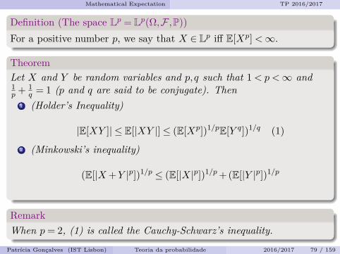
Definition (The space Lp = Lp(Ω,F ,P))For a positive number p, we say that X ∈ Lp iff E[Xp]<∞.
TheoremLet X and Y be random variables and p,q such that 1< p <∞ and1p + 1
q = 1 (p and q are said to be conjugate). Then1 (Holder’s Inequality)
|E[XY ]| ≤ E[|XY |]≤ (E[Xp])1/pE[Y q])1/q (1)2 (Minkowski’s inequality)
(E[|X+Y |p])1/p ≤ (E[|X|p])1/p+ (E[|Y |p])1/p
RemarkWhen p= 2, (1) is called the Cauchy-Schwarz’s inequality.
Patrıcia Goncalves (IST Lisbon) Teoria da probabilidade 2016/2017 79 / 159
Mathematical Expectation TP 2016/2017
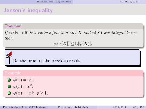
Jensen’s inequality
TheoremIf ϕ : R→ R is a convex function and X and ϕ(X) are integrable r.v.then
ϕ(E[X])≤ E[ϕ(X)].
Do the proof of the previous result.
Example1 ϕ(x) = |x|;2 ϕ(x) = x2;3 ϕ(x) = |x|p, p≥ 1.
Patrıcia Goncalves (IST Lisbon) Teoria da probabilidade 2016/2017 80 / 159
Mathematical Expectation TP 2016/2017
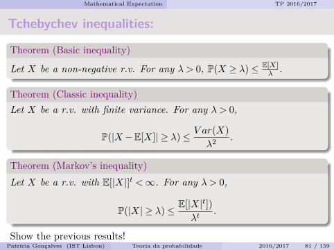
Tchebychev inequalities:
Theorem (Basic inequality)
Let X be a non-negative r.v. For any λ > 0, P(X ≥ λ)≤ E[X]λ .
Theorem (Classic inequality)Let X be a r.v. with finite variance. For any λ > 0,
P(|X−E[X]| ≥ λ)≤ V ar(X)λ2 .
Theorem (Markov’s inequality)Let X be a r.v. with E[|X|]t <∞. For any λ > 0,
P(|X| ≥ λ)≤ E[|X|t])λt
.
Show the previous results!Patrıcia Goncalves (IST Lisbon) Teoria da probabilidade 2016/2017 81 / 159
Mathematical Expectation TP 2016/2017
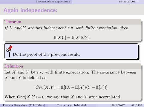
Again independence:
TheoremIf X and Y are two independent r.v. with finite expectation, then
E[XY ] = E[X]E[Y ].
Do the proof of the previous result.
DefinitionLet X and Y be r.v. with finite expectation. The covariance betweenX and Y is defined as
Cov(X,Y ) = E[(X−E[X])(Y −E[Y ])].
When Cov(X,Y ) = 0, we say that X and Y are uncorrelated.
Patrıcia Goncalves (IST Lisbon) Teoria da probabilidade 2016/2017 82 / 159
Mathematical Expectation TP 2016/2017
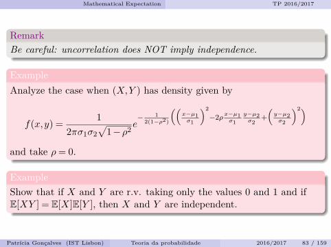
RemarkBe careful: uncorrelation does NOT imply independence.
ExampleAnalyze the case when (X,Y ) has density given by
f(x,y) = 12πσ1σ2
√1−ρ2 e
− 12(1−ρ2)
((x−µ1σ1
)2−2ρx−µ1
σ1y−µ2σ2
+(y−µ2σ2
)2)
and take ρ= 0.
ExampleShow that if X and Y are r.v. taking only the values 0 and 1 and ifE[XY ] = E[X]E[Y ], then X and Y are independent.
Patrıcia Goncalves (IST Lisbon) Teoria da probabilidade 2016/2017 83 / 159
Mathematical Expectation TP 2016/2017
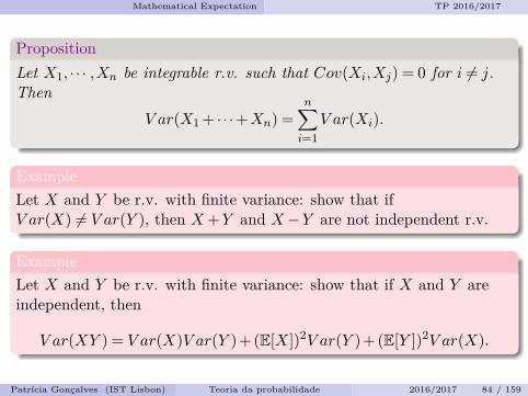
PropositionLet X1, · · · ,Xn be integrable r.v. such that Cov(Xi,Xj) = 0 for i 6= j.Then
V ar(X1 + · · ·+Xn) =n∑i=1
V ar(Xi).
ExampleLet X and Y be r.v. with finite variance: show that ifV ar(X) 6= V ar(Y ), then X+Y and X−Y are not independent r.v.
ExampleLet X and Y be r.v. with finite variance: show that if X and Y areindependent, then
V ar(XY ) = V ar(X)V ar(Y ) + (E[X])2V ar(Y ) + (E[Y ])2V ar(X).
Patrıcia Goncalves (IST Lisbon) Teoria da probabilidade 2016/2017 84 / 159

Convergence of sequences of r.v. TP 2016/2017
Convergence of sequences of r.v.
Patrıcia Goncalves (IST Lisbon) Teoria da probabilidade 2016/2017 85 / 159
Convergence of sequences of r.v. TP 2016/2017
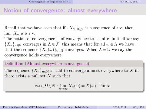
Notion of convergence: almost everywhere
Recall that we have seen that if Xnn≥1 is a sequence of r.v. thenlimnXn is a r.v.The notion of convergence is of convergence to a finite limit: if we sayXnn∈N converges in Λ ∈ F , this means that for all ω ∈ Λ we havethat the sequence Xn(ω)n∈N converges. When Λ = Ω we say theconvergence holds everywhere.
Definition (Almost everywhere convergence)The sequence Xnn∈N is said to converge almost everywhere to X iffthere exists a null set N such that
∀ω ∈ Ω\N : limn→∞
Xn(ω) =X(ω) finite.
Patrıcia Goncalves (IST Lisbon) Teoria da probabilidade 2016/2017 86 / 159
Convergence of sequences of r.v. TP 2016/2017
Convergence in probability
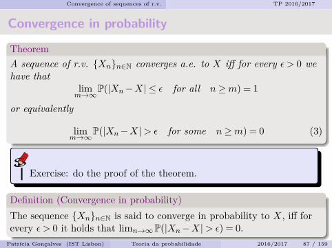
TheoremA sequence of r.v. Xnn∈N converges a.e. to X iff for every ε > 0 wehave that
limm→∞
P(|Xn−X| ≤ ε for all n≥m) = 1
or equivalently
limm→∞
P(|Xn−X|> ε for some n≥m) = 0 (3)
Exercise: do the proof of the theorem.
Definition (Convergence in probability)The sequence Xnn∈N is said to converge in probability to X, iff forevery ε > 0 it holds that limn→∞P(|Xn−X|> ε) = 0.
Patrıcia Goncalves (IST Lisbon) Teoria da probabilidade 2016/2017 87 / 159
Convergence of sequences of r.v. TP 2016/2017
Convergence a.e implies convergence in probability
TheoremConvergence a.e. to X implies convergence in probability to X.
Definition (Convergence in Lp, 0< p <∞)The sequence Xnn∈N is said to converge in Lp to X, iff Xn ∈ Lp,X ∈ Lp and
limn→∞
E[(|Xn−X|)p] = 0. (4)
DefinitionWe say that X is dominated by Y if |X| ≤ Y a.e. and that the sequenceis dominated by Y , if this is true for any n with the same Y . Moreover,if above Y is constant we say that X or Xn is uniformly bounded.
Above we can suppose X = 0 since the definitions hold for Xn−X.Patrıcia Goncalves (IST Lisbon) Teoria da probabilidade 2016/2017 88 / 159
Convergence of sequences of r.v. TP 2016/2017
Convergence in Lp implies convergence in probability
TheoremConvergence in Lp implies convergence in probability The converse istrue if the sequence is dominated by some Y ∈ Lp.
Convergence in probability does not imply convergence in Lp andconvergence in Lp does not imply convergence a.e.Convergence a.e. does not imply convergence in Lp.
Theorem (Scheffe’s Theorem)Let Xnn∈N be a sequence of r.v. with densities f1,f2, · · · and let X bea r.v. with density f . If limn fn = f, holds a.e. thenlimn→∞
∫R |fn−f |dx= 0.
Exercise: do the proof of the results above.
Patrıcia Goncalves (IST Lisbon) Teoria da probabilidade 2016/2017 89 / 159
Convergence of sequences of r.v. TP 2016/2017
The lim infnEn and the limsupnEnDefinitionSeja Enn∈N a sequence of subsets of Ω. The limsupnEn and theliminfnEn are defined by
limsupnEn = ∩∞m=1∪∞n=mEn and liminf
nEn = ∪∞m=1∩∞n=mEn (5)
RemarkNote that a point belongs to limsupnEn iff it belongs to infinitelymany terms of the sequence Enn∈N and belongs to liminfnEn iffit belongs to all the terms of the sequence from a certain point on.(Show this!)Also note that (limsupnEcn)c = liminfnEn.The event limsupnEn occurs iff the events En occur i.o.If each En ∈ F , then P(limsupnEn) = limm→∞P(∪∞n=mEn).
Patrıcia Goncalves (IST Lisbon) Teoria da probabilidade 2016/2017 90 / 159
Convergence of sequences of r.v. TP 2016/2017
Borel-Cantelli’s Lemma
Lemma (Borel-Cantelli - the convergent part)For Enn∈N arbitrary events, if
∑∞n=1P(En)<∞, then P(En i.o.) = 0.
We can rephrase the first theorem above:TheoremA sequence of r.v. Xnn≥1 converges a.e. to 0 iff ∀ε > 0P(|Xn|> ε i.o.) = 0.
TheoremIf Xnn≥1 converges in probability to X, then there exists a sequencenk of integers growing to ∞ such that Xn→X a.e. This means thatconvergence in probability implies converges a.e. along a subsequence.
Exercise: do the proof of the results.Patrıcia Goncalves (IST Lisbon) Teoria da probabilidade 2016/2017 91 / 159
Convergence of sequences of r.v. TP 2016/2017
If we add independence then we have
Lemma (Borel-Cantelli - the diververgent part)For independent events Enn∈N, if
∑∞n=1P(En) =∞, then
P(En i.o.) = 1.* The previous result also holds with pairwise independence. (We willnot see the proof in this case!)
RemarkRemoving the independence assumption, the result is false. TakeEn =A with 0< P(A)< 1.
CorollaryFor independent events Enn∈N, then P(En i.o.) = 0 or 1 if∑∞n=1P(En)<∞ or
∑∞n=1P(En) =∞
Exercise: do the proof of the results above.Patrıcia Goncalves (IST Lisbon) Teoria da probabilidade 2016/2017 92 / 159
Convergence of sequences of r.v. TP 2016/2017
The weak convergence
If a sequence of r.v. Xnn≥1 converges to some limit, does thesequence of probability distribution measures µnn∈N converges insome sense? Is is true that limnµn(A) exists for any A ∈ B? NO!!!And if µnn∈N converges in some sense, is the limit necessarily aprobability measure? NO!!!
DefinitionA p.m. µ in (R,B) with µ(R)≤ 1 is a called a subprobability measure.
Definition (Weak convergence)A sequence of subprobability measures µ in (R,B) is said to convergeweakly to a subprobability measure µ iff there exists a dense subset Dof R such that ∀a,b ∈D,a < b, limn→∞µn((a,b]) = µ((a,b]). We will usethe notation µn→v µ and µ is the weak limit (UNIQUE) of µnn∈N.
Patrıcia Goncalves (IST Lisbon) Teoria da probabilidade 2016/2017 93 / 159
Convergence of sequences of r.v. TP 2016/2017
DefinitionAn interval (a,b) is said to be a continuity interval of µ is a,b are notatoms of µ (that is µ((a,b)) = µ([a,b])).
LemmaLet µnn∈N and µ be subprobability measures. The followingpropositions are equivalent:
1 For every finite interval (a,b) and ε > 0, there exists an n0(a,b,ε)such that if n≥ n0, thenµ((a+ ε,b− ε))− ε≤ µn((a,b))≤ µ((a− ε,b+ ε)) + ε.
2 for every continuity interval (a,b] of µ we have thatlimn→∞µn((a,b]) = µ((a,b]).
3 µn→v µ.
Exercise: do the proof of the lemma.
Patrıcia Goncalves (IST Lisbon) Teoria da probabilidade 2016/2017 94 / 159
Convergence of sequences of r.v. TP 2016/2017
Helly’s extraction theorem
Recall that given any sequence of real numbers in a subset of [0,1],there is a subsequence which converges and the limit is an element ofthat set. (This means that [0,1] is sequentially compact). The set ofsubprobability measures is sequentially compact wrt the weakconvergence.
Theorem (Helly’s extraction theorem)Given any sequence of subprobability measures, there exists asubsequence that converges weakly to a subprobability measure.
Exercise: do the proof of the theorem.
Patrıcia Goncalves (IST Lisbon) Teoria da probabilidade 2016/2017 95 / 159
Convergence of sequences of r.v. TP 2016/2017
Uniqueness of the limit
DefinitionGiven Fn and F subdistribution functions, we say that Fn convergesweakly to F and we write Fn→v F if µn→v µ, where µn and µ are thesubprobability measures of Fn and F , respectively.
TheoremIf every weakly converging subsequence of a sequence µnn∈N ofsubprobability measures converges to the same µ, then µn→v µ.
TheoremLet µn and µ be subprobability measures. Then µn→v µ iff for allf ∈ Ck (or C0) we have that
∫R f(x)µn(dx)→n→∞
∫R f(x)µ(dx).
Exercise: do the proof of the results above.Patrıcia Goncalves (IST Lisbon) Teoria da probabilidade 2016/2017 96 / 159
Convergence of sequences of r.v. TP 2016/2017
Convergence in distribution
Definition (Convergence in distribution)A sequence of r.v. Xnn∈N is said to converge in distribution to F iffthe corresponding sequence of distribution functions Fnn∈Nconverges weakly to the distribution function F .
If X is a distribution function which has distribution function F , wewill say that Xnn∈N converges in distribution to X.
TheoremLet Fn and F be the distribution functions of the r.v. Xn and X. IfXnn∈N converges to X in probability, then Fn→n F . (Convergencein probability implies convergence in distribution).
Exercise: do the proof of the results above.
Patrıcia Goncalves (IST Lisbon) Teoria da probabilidade 2016/2017 97 / 159
Convergence of sequences of r.v. TP 2016/2017
LemmaLet c ∈ R. Then Xnn∈N converges to c in probability iff Xnn∈Nconverges to c in distribution.
When the limit is a constant, the convergence in probability isequivalent to the convergence in distribution.Note that it is not true that if Xnn∈N converges in distribution to Xand Ynn∈N converges in distribution to Y , the sum Xn+Ynn∈Nconverges in distribution to X+Y . But see the special case Y = 0!TheoremIf Xnn∈N converges in distribution to X and Ynn∈N converges indistribution to 0, then:
Xn+Ynn∈N converges in distribution to XXnYnn∈N converges in distribution to 0
Exercise: do the proof of the results above.Patrıcia Goncalves (IST Lisbon) Teoria da probabilidade 2016/2017 98 / 159

Law of Large Numbers TP 2016/2017
Law of Large Numbers
Patrıcia Goncalves (IST Lisbon) Teoria da probabilidade 2016/2017 99 / 159
Law of Large Numbers TP 2016/2017
Limit Theorems
The law of large numbers has to do with partial sums of a sequence ofr.v. Xnn≥1.
Sn :=X1 + · · ·+Xn
Weak/strong LawDepends on whether Sn−E[Sn]
n →n→∞ 0, in probability or a.e. (needsE[Sn] finite!)
RemarkWe have seen above that if a sequence converges to 0 in L2 then itconverges to 0 in probability and then it converges a.e. to 0 along asubsequence.
Patrıcia Goncalves (IST Lisbon) Teoria da probabilidade 2016/2017 100 / 159
Law of Large Numbers TP 2016/2017
Weak Law of Large Numbers (bounded secondmoments)
Theorem (Chebychev)If Xnn∈N is a sequence of uncorrelated r.v. whose second momentshave a common bound, then Sn−E[Sn]
n →n→∞ 0 in L2 and therefore alsoin probability.
Theorem (Rajchman)If Xnn∈N is a sequence of uncorrelated r.v. whose second momentshave a common bound, then Sn−E[Sn]
n →n→∞ 0 a.e.
Exercise: do the proof of the results above.
Patrıcia Goncalves (IST Lisbon) Teoria da probabilidade 2016/2017 101 / 159
Law of Large Numbers TP 2016/2017
Equivalent sequences (Kintchine)
DefinitionTwo sequences of r.v. Xnn≥1 and Ynn∈N are said to be equivalentiff∑n≥1P(Xn 6= Yn)<∞.
TheoremIf Xnn≥1 and Ynn∈N are equivalent then
∑n≥1(Xn−Yn) converges
a.e. Moreover, if an→+∞, then 1an
∑nj=1(Xj−Yj) converges a.e. to 0.
Theorem (Weak Law of Large Numbers of Kintchine)If Xnn≥1 is a sequence of pairwise independent and identicallydistributed r.v. with finite mean m, then Sn
n →m in probability.
Exercise: do the proof of the results.
Patrıcia Goncalves (IST Lisbon) Teoria da probabilidade 2016/2017 102 / 159
Law of Large Numbers TP 2016/2017
Strong Law of Large Numbers
Lemma (Kronecker’s Lemma)Let xkk≥1 a sequence of real numbers, akk≥1 a sequence of strictlypositive real numbers ↑∞. If
∑n≥1
xnan<∞, then 1
an
∑nj=1xj → 0.
TheoremLet ϕ : R→ R be a positive, even and continuous function, such that as|x| increases: ϕ(x)
|x| ↑ and ϕ(x)x2 ↓ . Let Xnn≥1 be a sequence of
independent r.v. with E[Xn] = 0 for every n and let 0< an ↑+∞. If∑n≥1
E[ϕ(Xn)]ϕ(an) <∞, then
∑n≥1
Xnan
converges a.e.
Exercise: do the proof of the theorem.
Patrıcia Goncalves (IST Lisbon) Teoria da probabilidade 2016/2017 103 / 159
Law of Large Numbers TP 2016/2017
Strong Law of Large Numbers (Kolmogorov)
TheoremLet Xnn≥1 be a sequence of independent and identically distributedr.v., then
E[|X1|]<∞⇒Snn→ E[X1] a.e.
E[|X1|] =∞⇒ limsupn
|Sn|n
= +∞ a.e.
Exercise: do the proof of the theorem.
Patrıcia Goncalves (IST Lisbon) Teoria da probabilidade 2016/2017 104 / 159

Characteristic functions TP 2016/2017
Characteristic functions
Patrıcia Goncalves (IST Lisbon) Teoria da probabilidade 2016/2017 105 / 159
Characteristic functions TP 2016/2017
Characteristic functions
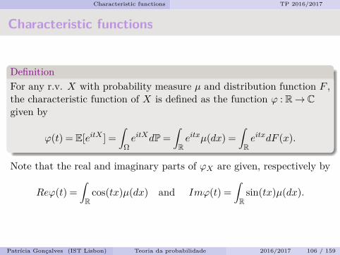
DefinitionFor any r.v. X with probability measure µ and distribution function F ,the characteristic function of X is defined as the function ϕ : R→ Cgiven by
ϕ(t) = E[eitX ] =∫
ΩeitXdP =
∫Reitxµ(dx) =
∫ReitxdF (x).
Note that the real and imaginary parts of ϕX are given, respectively by
Reϕ(t) =∫R
cos(tx)µ(dx) and Imϕ(t) =∫R
sin(tx)µ(dx).
Patrıcia Goncalves (IST Lisbon) Teoria da probabilidade 2016/2017 106 / 159
Characteristic functions TP 2016/2017
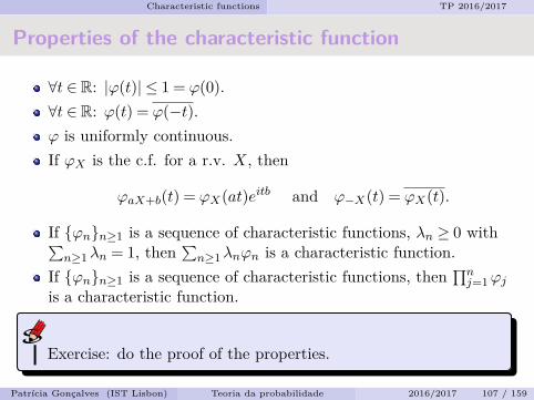
Properties of the characteristic function
∀t ∈ R: |ϕ(t)| ≤ 1 = ϕ(0).∀t ∈ R: ϕ(t) = ϕ(−t).ϕ is uniformly continuous.If ϕX is the c.f. for a r.v. X, then
ϕaX+b(t) = ϕX(at)eitb and ϕ−X(t) = ϕX(t).
If ϕnn≥1 is a sequence of characteristic functions, λn ≥ 0 with∑n≥1λn = 1, then
∑n≥1λnϕn is a characteristic function.
If ϕnn≥1 is a sequence of characteristic functions, then∏nj=1ϕj
is a characteristic function.
Exercise: do the proof of the properties.
Patrıcia Goncalves (IST Lisbon) Teoria da probabilidade 2016/2017 107 / 159
Characteristic functions TP 2016/2017
The sum of random variables
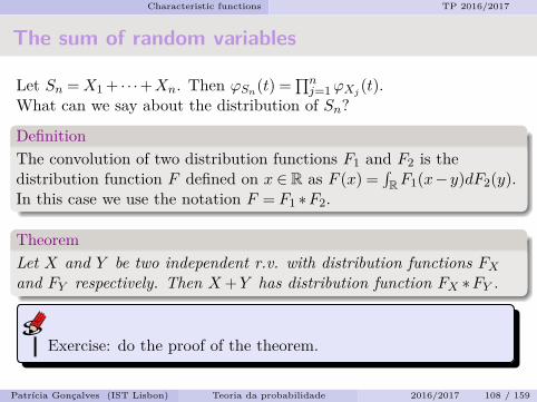
Let Sn =X1 + · · ·+Xn. Then ϕSn(t) =∏nj=1ϕXj (t).
What can we say about the distribution of Sn?
DefinitionThe convolution of two distribution functions F1 and F2 is thedistribution function F defined on x ∈ R as F (x) =
∫RF1(x−y)dF2(y).
In this case we use the notation F = F1 ∗F2.
TheoremLet X and Y be two independent r.v. with distribution functions FXand FY respectively. Then X+Y has distribution function FX ∗FY .
Exercise: do the proof of the theorem.
Patrıcia Goncalves (IST Lisbon) Teoria da probabilidade 2016/2017 108 / 159
Characteristic functions TP 2016/2017
The convolution
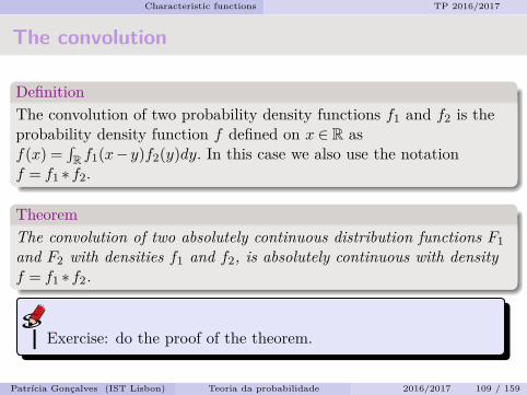
DefinitionThe convolution of two probability density functions f1 and f2 is theprobability density function f defined on x ∈ R asf(x) =
∫R f1(x−y)f2(y)dy. In this case we also use the notation
f = f1 ∗f2.
TheoremThe convolution of two absolutely continuous distribution functions F1and F2 with densities f1 and f2, is absolutely continuous with densityf = f1 ∗f2.
Exercise: do the proof of the theorem.
Patrıcia Goncalves (IST Lisbon) Teoria da probabilidade 2016/2017 109 / 159
Characteristic functions TP 2016/2017
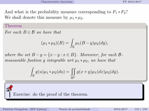
And what is the probability measure corresponding to F1 ∗F2?We shall denote this measure by µ1 ∗µ2.
TheoremFor each B ∈ B we have that
(µ1 ∗µ2)(B) =∫Rµ1(B−y)µ2(dy),
where the set B−y = x−y : x ∈B. Moreover, for each B-measurable funtion g integrable wrt µ1 ∗µ2, we have that∫
Rg(u)µ1 ∗µ2(du) =
x
R2
g(x+y)µ1(dx)µ2(dy).
Exercise: do the proof of the theorem.
Patrıcia Goncalves (IST Lisbon) Teoria da probabilidade 2016/2017 110 / 159
Characteristic functions TP 2016/2017
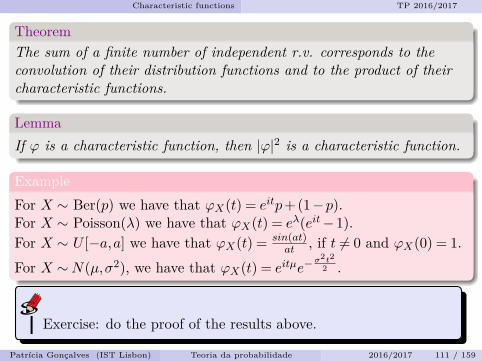
TheoremThe sum of a finite number of independent r.v. corresponds to theconvolution of their distribution functions and to the product of theircharacteristic functions.
LemmaIf ϕ is a characteristic function, then |ϕ|2 is a characteristic function.
ExampleFor X ∼ Ber(p) we have that ϕX(t) = eitp+ (1−p).For X ∼ Poisson(λ) we have that ϕX(t) = eλ(eit−1).For X ∼ U [−a,a] we have that ϕX(t) = sin(at)
at , if t 6= 0 and ϕX(0) = 1.For X ∼N(µ,σ2), we have that ϕX(t) = eitµe−
σ2t22 .
Exercise: do the proof of the results above.
Patrıcia Goncalves (IST Lisbon) Teoria da probabilidade 2016/2017 111 / 159
Characteristic functions TP 2016/2017
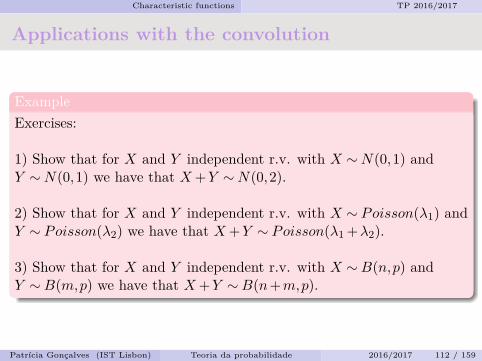
Applications with the convolution
ExampleExercises:
1) Show that for X and Y independent r.v. with X ∼N(0,1) andY ∼N(0,1) we have that X+Y ∼N(0,2).
2) Show that for X and Y independent r.v. with X ∼ Poisson(λ1) andY ∼ Poisson(λ2) we have that X+Y ∼ Poisson(λ1 +λ2).
3) Show that for X and Y independent r.v. with X ∼B(n,p) andY ∼B(m,p) we have that X+Y ∼B(n+m,p).
Patrıcia Goncalves (IST Lisbon) Teoria da probabilidade 2016/2017 112 / 159
Characteristic functions TP 2016/2017
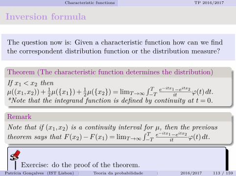
Inversion formula
The question now is: Given a characteristic function how can we findthe correspondent distribution function or the distribution measure?
Theorem (The characteristic function determines the distribution)If x1 < x2 thenµ((x1,x2)) + 1
2µ(x1) + 12µ(x2) = limT→∞
∫ T−T
e−itx1−eitx2it ϕ(t)dt.
*Note that the integrand function is defined by continuity at t= 0.
RemarkNote that if (x1,x2) is a continuity interval for µ, then the previoustheorem says that F (x2)−F (x1) = limT→∞
∫ T−T
e−itx1−eitx2it ϕ(t)dt.
Exercise: do the proof of the theorem.Patrıcia Goncalves (IST Lisbon) Teoria da probabilidade 2016/2017 113 / 159
Characteristic functions TP 2016/2017
Uniqueness of distribution
TheoremIf two probability measures (or two distribution functions) have thesame characteristic function, then the probability measures (or thedistribution functions) are the same.
TheoremIf ϕ ∈ L1(−∞,+∞), then F ∈ C1 and F ′(x) = 1
2π∫+∞−∞ e−ixtϕ(t)dt, that
is ϕ is the characteristic function of an absolutely continuous r.v.
CorollaryIf ϕ ∈ L1(−∞,+∞), then p(x) ∈ L1 where p(x) = 1
2π∫+∞−∞ e−ixtϕ(t)dt
and ϕ(x) =∫∞−∞ e
itxp(x)dx.
Exercise: do the proof of the results.Patrıcia Goncalves (IST Lisbon) Teoria da probabilidade 2016/2017 114 / 159
Characteristic functions TP 2016/2017
The atoms of µ
Theorem• For each x0 we have that
limT→∞
12T
∫ T
−Te−itX0ϕ(t)dt= µ(x0).
• It holds that
limT→∞
12T
∫ T
−T|ϕ(t)|2 dt=
∑x∈R
(µ(x))2.
Theoremµ is atomless (F is continuous) iff limT→∞
12T∫ T−T |ϕ(t)|2 dt= 0.
Exercise: do the proof of the results above.Patrıcia Goncalves (IST Lisbon) Teoria da probabilidade 2016/2017 115 / 159
Characteristic functions TP 2016/2017
Symmetric random variables
DefinitionWe say that a r.v. X is symmetric around 0 iff X and −X have thesame distribution.
RemarkFor a symmetric r.v. its distribution µ has the following propertyµ(B) = µ(−B) for any B ∈ B. Such probability measure is said to besymmetric around 0. Equivalently, for the distribution function, wehave that for any x ∈ R, F (x) = 1−F (x−).
TheoremA r.v. X or a p.m. µ is symmetric iff its characteristic function isreal-valued (for all t.)
Exercise: do the proof of the theorem.Patrıcia Goncalves (IST Lisbon) Teoria da probabilidade 2016/2017 116 / 159
Characteristic functions TP 2016/2017
Convergence theorems
Theorem (Levy’s converging Theorem)Let µn n≥ 1 and µ∞ be subprobability measures on R withcharacteristic function ϕnn≥1.
It µn→v µ∞, then ϕn(t)→n→∞ ϕ∞(t), where ϕ∞ is thecharacteristic function of µ∞.If ϕn(t)→n→∞ ϕ∞(t) for all t ∈ R, and ϕ∞(t) is continuous att= 0, then
ϕ∞ is a characteristic function of a r.v.µn→v µ∞ and ϕ∞ is the characteristic function of µ∞.
Exercise: do the proof of the theorem.
Patrıcia Goncalves (IST Lisbon) Teoria da probabilidade 2016/2017 117 / 159
Characteristic functions TP 2016/2017
CorollaryIf µn n≥ 1 and µ are probability measures with characteristicfunctions ϕnn≥1 and ϕ, then µn→v µ∞ iff ϕn(t)→n→∞ ϕ(t), for allt ∈ R.
Exercise: do the proof of the corollary.
ExampleExercises:1) Take µn which gives mass 1/2 to 0 and to n and analyze it.2) Take µn as Uniform in [−n,n] and analyze it.
Patrıcia Goncalves (IST Lisbon) Teoria da probabilidade 2016/2017 118 / 159
Characteristic functions TP 2016/2017
Applications
TheoremIf F has finite absolute moment of order k, with k ≥ 1, then ϕ has thefollowing expansion around a neighbourhood of t= 0:
ϕ(t) =k∑j=0
ij
j!mjtj +o(|t|k)
ϕ(t) =k−1∑j=0
ij
j!mjtj + θk
k!µk|t|k,
where mj is the moment of order j, µk is the absolute moment of orderk and θk ≤ 1.
Patrıcia Goncalves (IST Lisbon) Teoria da probabilidade 2016/2017 119 / 159
Characteristic functions TP 2016/2017
Applications: limiting laws
Theorem (The weak law of large numbers)
If F has finite mean m<∞, then Snn →m in probability.
Theorem (The central limit theorem)If F has finite mean m<∞ and variance σ2 such that 0< σ2 <+∞,then Sn−mn
σ√n→ Φ in distribution, where Φ is the distribution function of
N(0,1).
Exercise: do the proof of the results above.
Patrıcia Goncalves (IST Lisbon) Teoria da probabilidade 2016/2017 120 / 159

Conditional expectation TP 2016/2017
Conditional expectation
Patrıcia Goncalves (IST Lisbon) Teoria da probabilidade 2016/2017 121 / 159
Conditional expectation TP 2016/2017
Definition (Conditional probability)Given a set A ∈ F with P(A)> 0 we define PA(·) in the following way:
PA(E) = P(A∩E)P(A) .
PA is a probability measure and it is called the conditional probabilitywith respect to A. The expectation with respect to this probability iscalled the conditional expectation wrt A:
EA[X] =∫
ΩX(ω)PA(dω) = 1
P(A)
∫AX(ω)P(dω).
DefinitionIf we take now a partition of Ω that is (An)n≥1 with Ω = ∪n≥1An,An ∈ F and An∩Am = ∅ if m 6= n, then given a set E ∈ F we have that
P(E) =∑n≥1
P(E∩An) =∑n≥1
PAn(E)P(An).
Patrıcia Goncalves (IST Lisbon) Teoria da probabilidade 2016/2017 122 / 159
Conditional expectation TP 2016/2017
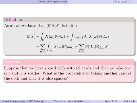
DefinitionAs above we have that (if E[X] is finite)
E[X] =∫
ΩX(ω)P(dω) =
∫∪n≥1AnX(ω)P(dω)
=∑n≥1
∫AnX(ω)P(dω) =
∑n≥1
P(An)EAn [X].
ExampleSuppose that we have a card deck with 52 cards and that we take oneout and it is spades. What is the probability of taking another card ofthe deck and that it is also spades?
Patrıcia Goncalves (IST Lisbon) Teoria da probabilidade 2016/2017 123 / 159
Conditional expectation TP 2016/2017
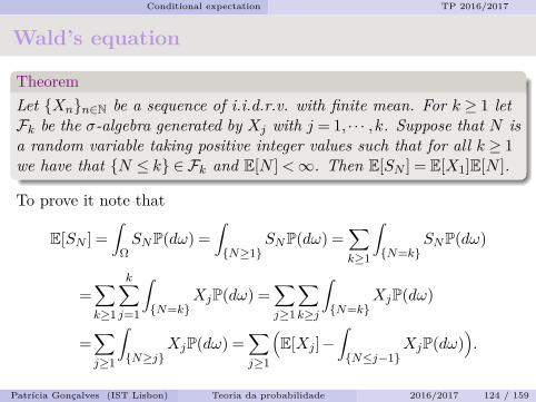
Wald’s equation
TheoremLet Xnn∈N be a sequence of i.i.d.r.v. with finite mean. For k ≥ 1 letFk be the σ-algebra generated by Xj with j = 1, · · · ,k. Suppose that N isa random variable taking positive integer values such that for all k ≥ 1we have that N ≤ k ∈ Fk and E[N ]<∞. Then E[SN ] = E[X1]E[N ].
To prove it note that
E[SN ] =∫
ΩSNP(dω) =
∫N≥1
SNP(dω) =∑k≥1
∫N=k
SNP(dω)
=∑k≥1
k∑j=1
∫N=k
XjP(dω) =∑j≥1
∑k≥j
∫N=k
XjP(dω)
=∑j≥1
∫N≥j
XjP(dω) =∑j≥1
(E[Xj ]−
∫N≤j−1
XjP(dω)).
Patrıcia Goncalves (IST Lisbon) Teoria da probabilidade 2016/2017 124 / 159
Conditional expectation TP 2016/2017
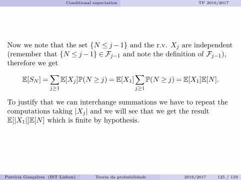
Now we note that the set N ≤ j−1 and the r.v. Xj are independent(remember that N ≤ j−1 ∈ Fj−1 and note the definition of Fj−1),therefore we get
E[SN ] =∑j≥1
E[Xj ]P(N ≥ j) = E[X1]∑j≥1
P(N ≥ j) = E[X1]E[N ].
To justify that we can interchange summations we have to repeat thecomputations taking |Xj | and we will see that we get the resultE[|X1|]E[N ] which is finite by hypothesis.
Patrıcia Goncalves (IST Lisbon) Teoria da probabilidade 2016/2017 125 / 159
Conditional expectation TP 2016/2017
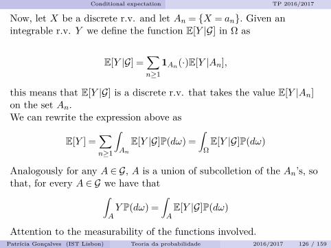
Now, let X be a discrete r.v. and let An = X = an. Given anintegrable r.v. Y we define the function E[Y |G] in Ω as
E[Y |G] =∑n≥1
1An(·)E[Y |An],
this means that E[Y |G] is a discrete r.v. that takes the value E[Y |An]on the set An.We can rewrite the expression above as
E[Y ] =∑n≥1
∫An
E[Y |G]P(dω) =∫
ΩE[Y |G]P(dω)
Analogously for any A ∈ G, A is a union of subcolletion of the An’s, sothat, for every A ∈ G we have that∫
AY P(dω) =
∫AE[Y |G]P(dω)
Attention to the measurability of the functions involved.Patrıcia Goncalves (IST Lisbon) Teoria da probabilidade 2016/2017 126 / 159
Conditional expectation TP 2016/2017
Now, we suppose that we have two functions ϕ1 and ϕ2 both Gmeasurable and such that∫
AY P(dω) =
∫Aϕ1P(dω) =
∫Aϕ2P(dω).
If we take the set A= ω ∈ Ω : ϕ1(ω)> ϕ2(ω), then A ∈ G and weconclude that P(A) = 0. Repeating the argument exchanging ϕ1 withϕ2 we conclude that ϕ1 = ϕ2 a.e.
This means that E[Y |G] is unique up to a equivalence and we are goingto denote EG [Y ] or E[Y |G] to denote that class. The results holds forany σ-algebra.
TheoremIf E[|Y |]<∞ and G is a σ-algebra contained in F , then, there exists aunique equivalence class of integrable r.v. E[Y |G] belonging to G suchthat for any A ∈ G it holds that
∫AY P(dω) =
∫AE[Y |G]P(dω).
Patrıcia Goncalves (IST Lisbon) Teoria da probabilidade 2016/2017 127 / 159
Conditional expectation TP 2016/2017
Conditional expectation
Definition (Conditional expectation)Given an integrable r.v. Y and a σ-algebra G, the conditionalexpectation EG [Y ] of Y with respect to G is any one of the equivalenceclass of r.v. on Ω such that:
1 it belongs to G;2 it has the same integral as Y over any set in G.
Note that for Y = 1Λ with Λ ∈ F we write P(Λ|G) = E[1Λ|G] and this isthe conditional probability of Λ relatively to G. This is any one of theequivalence class of r.v. belonging to G and satisfying
∀B ∈ G : P(B∩Λ) =∫BP(Λ|G)P(dω).
Patrıcia Goncalves (IST Lisbon) Teoria da probabilidade 2016/2017 128 / 159
Conditional expectation TP 2016/2017
Conditional expectation
TheoremLet Y and ZY be integrable r.v. and let Z ∈ G. Then
E[Y Z|G] = ZE[Y |G], a.e.
Exercise: do the proof of the theorem.
Let us note that E[X|T ] = E[X], where T is the trivial σ-algebra, thatis T := ∅,Ω.
Patrıcia Goncalves (IST Lisbon) Teoria da probabilidade 2016/2017 129 / 159
Conditional expectation TP 2016/2017
Properties of the conditional expectation
Let X and Xn be integrable r.v.1 If X ∈ G, then E[X|G] =X a.e., this is true also if X = a a.e.,2 E[X1 +X2|G] = E[X1|G] +E[X2|G],3 If X1 ≤X2 then E[X1|G]≤ E[X2|G],4 |E[X|G]| ≤ E[|X||G],5 If Xn ↑X, then E[Xn|G] ↑ E[X|G],6 If Xn ↓X, then E[Xn|G] ↓ E[X|G],7 If |Xn| ≤ Y , Y is integrable and Xn→X, then E[Xn|G]→ E[X|G],8 E[|XY ||G]2 ≤ E[X2|G]E[Y 2|G]. (Cauchy-Schwarz inequality)
Exercise: do the proof.Patrıcia Goncalves (IST Lisbon) Teoria da probabilidade 2016/2017 130 / 159
Conditional expectation TP 2016/2017
Jensen’s inequality
Theorem (Jensen’s inequality)If ϕ is a convex function on R and X and ϕ(X) are integrable r.v.,then for each G:
ϕ(E[X|G])≤ E[ϕ(X)|G].
Exercise: do the proof.
Note that when Λ = Ω, the defining relation for the conditionalexpectation says that
E[E[Y |G]|T ] = E[Y |T ] = E[E[Y |T ]|G]
This can be generalized and it is called the tower law.
Patrıcia Goncalves (IST Lisbon) Teoria da probabilidade 2016/2017 131 / 159
Conditional expectation TP 2016/2017
Tower Law
Theorem (Tower law)If Y is integrable and F1 ⊂F2, then:
E[Y |F1] = E[Y |F2] iff E[Y |F2] ∈ F1.E[E[Y |F2]|F1] = E[Y |F1] = E[E[Y |F1]|F2]
As a particular case we note that
E[E[Y |X1,X2]|X1] = E[Y |X1] = E[E[Y |X1]|X1,X2].
Patrıcia Goncalves (IST Lisbon) Teoria da probabilidade 2016/2017 132 / 159
Conditional expectation TP 2016/2017
Tower Law: proof of the theoremLet us prove the theorem now.
We start with the first assertion. Let start by assuming thatE[Y |F1] = E[Y |F2], then by 1) in page 128 we have that E[Y |F2] ∈ F1.Now let us assume that E[Y |F2] ∈ F1. Then, for A ∈ F1, 2) in page 128holds, from where the result follows.
Now let us prove the second assertion. Note that E[Y |F1] ∈ F2, andfrom the first assertion applied to E[Y |F1] we conclude the secondequality. Let us prove the first equality now. For that purpose notethat if Λ ∈ F1 then Λ ∈ F2, so that∫
ΛE[E[Y |F2]|F1]P(dω) =
∫ΛE[Y |F2]P(dω) =
∫ΛY P(dω).
Moreover, E[E[Y |F2]|F1] ∈ F1 so that, both properties defining theconditional expectation are verified and we are done.
Patrıcia Goncalves (IST Lisbon) Teoria da probabilidade 2016/2017 133 / 159
Conditional expectation TP 2016/2017
Conditional independence
Let F be a σ-algebra and let Fαα∈A, where A is a index set, becontained in F .DefinitionThe collection Fαα∈A is said to be conditionally independent to aσ-algebra G iff for any finite collection of sets A1, · · · ,An with Aj ∈ Fjand with α′js distinct indices of A we have
P(∩nj=1Aj |G
)=
n∏j=1
P(Aj |G).
Note that if G = T then the previous condition is just the usualindependence.
Patrıcia Goncalves (IST Lisbon) Teoria da probabilidade 2016/2017 134 / 159
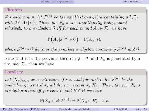
Conditional expectation TP 2016/2017
TheoremFor each α ∈A, let F (α) be the smallest σ-algebra containing all Fβwith β ∈A\α. Then, the Fα’s are conditionally independentrelatively to a σ-algebra G iff for each α and Aα ∈ Fα we have
P(Aα|F (α)∨G
)= P(Aα|G),
where F (α)∨G denotes the smallest σ-algebra containing F (α) and G.
Note that if in the previous theorem G = T and Fα is generated by ar.v. say Xα then we have
CorollaryLet (Xα)α∈A be a collection of r.v. and for each α let F (α) be theσ-algebra generated by all the r.v. except by Xα. Then, the r.v. Xα’sare independent iff for each α and B ∈ B we have
P(Xα ∈B|F (α)) = P(Xα ∈B) a.e.
Patrıcia Goncalves (IST Lisbon) Teoria da probabilidade 2016/2017 135 / 159
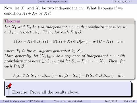
Conditional expectation TP 2016/2017
Now, let X1 and X2 be two independent r.v. What happens if wecondition X1 +X2 by X1?
TheoremLet X1 and X2 be two independent r.v. with probability measures µ1and µ2, respectively. Then, for each B ∈ B:
P(X1 +X2 ∈B|X1) = P(X1 +X2 ∈B|F1) = µ2(B−X1) a.e.
where F1 is the σ−algebra generated by X1.More generally, let (Xn)n∈N be a sequence of independent r.v. withprobability measures (µn)n∈N and let Sn =X1 + · · ·+Xn. Then, foreach B ∈ B:
P(Sn ∈B|S1, · · · ,Sn−1) = µn(B−Sn1) = P(Sn ∈B|Sn−1) a.e.
Exercise: Prove all the results above.
Patrıcia Goncalves (IST Lisbon) Teoria da probabilidade 2016/2017 136 / 159
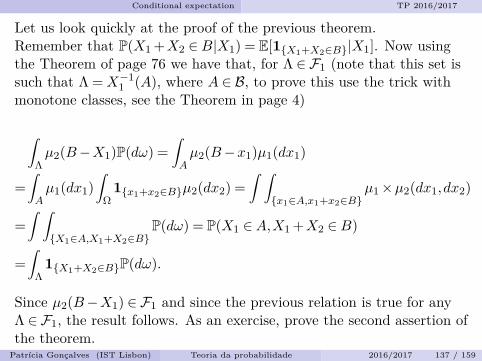
Conditional expectation TP 2016/2017
Let us look quickly at the proof of the previous theorem.Remember that P(X1 +X2 ∈B|X1) = E[1X1+X2∈B|X1]. Now usingthe Theorem of page 76 we have that, for Λ ∈ F1 (note that this set issuch that Λ =X−1
1 (A), where A ∈ B, to prove this use the trick withmonotone classes, see the Theorem in page 4)
∫Λµ2(B−X1)P(dω) =
∫Aµ2(B−x1)µ1(dx1)
=∫Aµ1(dx1)
∫Ω
1x1+x2∈Bµ2(dx2) =∫ ∫x1∈A,x1+x2∈B
µ1×µ2(dx1,dx2)
=∫ ∫X1∈A,X1+X2∈B
P(dω) = P(X1 ∈A,X1 +X2 ∈B)
=∫
Λ1X1+X2∈BP(dω).
Since µ2(B−X1) ∈ F1 and since the previous relation is true for anyΛ ∈ F1, the result follows. As an exercise, prove the second assertion ofthe theorem.
Patrıcia Goncalves (IST Lisbon) Teoria da probabilidade 2016/2017 137 / 159
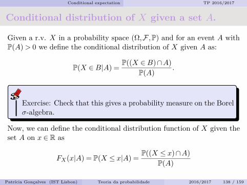
Conditional expectation TP 2016/2017
Conditional distribution of X given a set A.
Given a r.v. X in a probability space (Ω,F ,P) and for an event A withP(A)> 0 we define the conditional distribution of X given A as:
P(X ∈B|A) = P((X ∈B)∩A)P(A) .
Exercise: Check that this gives a probability measure on the Borelσ-algebra.
Now, we can define the conditional distribution function of X given theset A on x ∈ R as
FX(x|A) = P(X ≤ x|A) = P((X ≤ x)∩A)P(A)
Patrıcia Goncalves (IST Lisbon) Teoria da probabilidade 2016/2017 138 / 159
Conditional expectation TP 2016/2017
The conditional expectation of X given the set A is the expectation ofthe conditional distribution given by
E[X|A] =∫xdFX(x|A)
if it exists. As above, if we take now a partition of Ω that is (An)n≥1with Ω = ∪n≥1An, An ∈ F and An∩Am = ∅ if m 6= n, then
P(X ∈B) =∑n≥1
P(X ∈B|An)P(An).
Also for any x,FX(x) = P(X ≤ x) =
∑n≥1P(X ≤ x|An)P(An) =
∑n≥1FX(x|An)P(An)
and analogously
E[X] =∫xdFX(x) =
∑n≥1
P(An)E[X|An].
1) Let X ∼ U [−1,1] and let A= X ≥ 0. What is the conditionaldistribution of X given A?
Patrıcia Goncalves (IST Lisbon) Teoria da probabilidade 2016/2017 139 / 159
Conditional expectation TP 2016/2017
Conditional distribution of X given a discreter.v. YLet us suppose now that the partition is generated by a discrete r.v.Let Y be a discrete r.v. defined on a probability space (Ω,F ,P) takingthe values (an)n∈N. Then the events Y = an form a partition of Ω. Inthis case P(X ∈B|Y = an) is called the conditional distribution of Xgiven Y = an and we have that
P(X ∈B|Y = an) =∑n≥1
P(X ∈B|Y = an)P(Y = an).
Also for any x,
FX(x) = P(X ≤ x) =∑n≥1
P(X ≤ x|Y = an)P(Y = an)
=∑n≥1
FX(x|Y = an)P(X = an)
and analogously E[X] =∫xdFX(x) =
∑n≥1P(Y = an)E[X|Y = an].
Patrıcia Goncalves (IST Lisbon) Teoria da probabilidade 2016/2017 140 / 159
Conditional expectation TP 2016/2017
Note that for B fixed we have that P(X ∈B|Y = an) is a function of anlet us say g(an). Defining g(y) = P(X ∈B|Y = y) we have thatP(X ∈B) =
∫P(X ∈B|Y = y)dFY (y) =
∫g(y)dFY (y). Moreover,
FX(x) =∫FX(x|Y = y)dFY (y) E[X] =
∫E[X|Y = y]dFY (y).
When X is integrable the function ϕ(y) = E[X|Y = y] is finite. In thiscase, the r.v. ϕ(Y ) is called the conditional expectation of X given Y :ϕ(Y ) = E[X|Y ]. We note that E[X|Y = y] is the value of the randomvariable E[X|Y ] when Y = y. The last formula can be interpreted as
E[X] = E[ϕ(Y )] = E[E[X|Y ]].
2) Consider the following experience: a player tosses a fair coin n timesobtaining k heads with 0≤ k ≤ n. After that a second player tosses thesame coin k times. Let X be the number of heads obtained by thesecond player. What is the expectation of X supposing that all theevents are independent?
Patrıcia Goncalves (IST Lisbon) Teoria da probabilidade 2016/2017 141 / 159
Conditional expectation TP 2016/2017
Conditional distribution: general case
Let us define now the conditional expectation for general r.v. X andY . Before we defined the conditional distribution of X when Y wasdiscrete, so that P(Y = y) = 0 for all y 6= an. But now we want toextend this to the continuous case in which the probability above isnull for all y ∈ R. How to do it? We define by approximation. Take Ian interval containing y with size ∆y and define
P(X ∈B|Y = y)∼ P(X ∈B|Y ∈ I) = P(X ∈B,Y ∈ I)P(Y ∈ I) .
If P(X ∈B|Y ∈ I) has a limit when ∆y→ 0 we call to the limitP(X ∈B|Y = y):
lim∆y→0
P(X ∈B|Y ∈ I) = P(X ∈B|Y = y).
Patrıcia Goncalves (IST Lisbon) Teoria da probabilidade 2016/2017 142 / 159
Conditional expectation TP 2016/2017
Let us go back to the case in which X is discrete.Then we have
F(X,Y )(x,y) = P(X ≤ x,Y ≤ y) =∑
n:an≤yP(X ≤ x,Y = an)
=∑
n:an≤yP(X ≤ x|Y = an)P(Y = an)
=∑
n:an≤yFX(x|Y = an)P(Y = an)
=∫ y
−∞FX(x|Y = a)dFY (a).
Note that in the discrete case, the joint distribution is like acomposition of the marginal distribution of Y with the conditionaldistribution of X given Y . Let use then the last equality!
Patrıcia Goncalves (IST Lisbon) Teoria da probabilidade 2016/2017 143 / 159
Conditional expectation TP 2016/2017
Formal definitions
DefinitionLet X and Y be two r.v. defined on the same probability space. Afunction P(X ∈B|Y = y) defined for each borelian B and y ∈ R is a(regular) conditional distribution for X given Y if:
1 for each y fixed, P(X ∈B|Y = y) defines a probability measure inB,
2 for any B ∈ B fixed, P(X ∈B|Y = y) is a measurable function of y,3 for any (x,y) ∈ R2 it holds that
P(X ≤ x,Y ≤ y) =∫ y
−∞FX(x|Y = a)dFY (a).
P(X ∈B|Y = y) is called the conditional probability of X belonging toB given that Y = y and FX(·|Y = y) = P(X ≤ ·|Y = y) is theconditional distribution of X given Y = y.
Patrıcia Goncalves (IST Lisbon) Teoria da probabilidade 2016/2017 144 / 159
Conditional expectation TP 2016/2017
Formal definitions
TheoremLet X and Y be two r.v. defined on the same probability space. Thereexists a (regular) conditional distribution for X given Y . In fact thereexists only one in the sense that they are equal a.e.: that is, ifP1(X ∈B|Y = y) and P2(X ∈B|Y = y) are conditional distributionsfor X given Y , then there exists a borelian B0 such that P(Y ∈B0) = 1and P1(X ∈B|Y = y) = P2(X ∈B|Y = y) for all B ∈ B and y ∈B0.
TheoremFor each B ∈ B fixed, the limit
lim∆a→0
P(X ∈B|Y ∈ I) = P(X ∈B|Y = a)
exists a.e. Moreover, for each B ∈ B fixed, the limit is equal toP(X ∈B|X = y) as given in the definition above, a.e.
Patrıcia Goncalves (IST Lisbon) Teoria da probabilidade 2016/2017 145 / 159
Conditional expectation TP 2016/2017
1) What is the conditional distribution of Y given Y ? Let us guess it.If it is given that Y = y, then Y = y! So the candidate isP(Y = y|Y = y) = 1 the distribution which gives weight 1 to the pointy. Check that for B = (q1, q2) with qi ∈Q it holds that
P(Y ∈B|Y = y) = lim∆a→0
P(Y ∈B|Y ∈ I),
which proves the result.Note however that if we take B = y0 then
P(Y = y0|Y = y) = lim∆a→0
P(Y = y0|Y ∈ I) = 0!
This does not contradict our result but contradicts our intuition!2) Given Y = y what is the conditional distribution of Z = g(Y )? Recallthat above we have seen that if Y = y, then P(Y = y|Y = y) = 1. Hereit is analogous. In this case we have that P(g(Y ) = g(y)|Y = y) = 1.
Patrıcia Goncalves (IST Lisbon) Teoria da probabilidade 2016/2017 146 / 159
Conditional expectation TP 2016/2017
3) Let X be a symmetric r.v. around 0. What is the conditionaldistribution of X given the r.v. |X|? Given that |X|= y > 0, thenX = y or −y, there are no other possibilities and from symmetry wehave that:
P(X = y||X|= y) = 12 = P(X =−y||X|= y), y > 0,
and P(X = 0||X|= 0) = 1.Let us do it now in a different way. Suppose y > 0. Take B = (q1,a2)with qi ∈Q and take I ⊂B. Then
P(X ∈B||X| ∈ I) =P(X ∈ I) = 12(P(X ∈ I)+P(X ∈−I)
)= 1
2P(|X| ∈ I).
And
P(X ∈ −B||X| ∈ I) = P(X ∈ −I) = 12P(|X| ∈ I).
Patrıcia Goncalves (IST Lisbon) Teoria da probabilidade 2016/2017 147 / 159
Conditional expectation TP 2016/2017
Since I ⊂B we have that
P(X ∈B||X| ∈ I) = 12 = P(X ∈ −B||X| ∈ I).
Therefore,
P(X ∈B||X|= y) = lim∆y→0
P(X ∈B||X| ∈ I) = 12 ,
P(X ∈ −B||X|= y) = lim∆y→0
P(X ∈ −B||X| ∈ I) = 12 .
Taking B decreasing to y we see that the conditional probabilitygives weight 1/2 to each one of the points y and −y. The proof thatP(X = 0||X|= 0) = 1 can be reached by taking B = (q1, q2) as abovewith q1 < 0< q2.
Patrıcia Goncalves (IST Lisbon) Teoria da probabilidade 2016/2017 148 / 159
Conditional expectation TP 2016/2017
4) Let X and Y be independent r.v. each one with law N(0,σ2) withσ2 > 0. What is the conditional distribution of (X,Y ) given
√X2 +Y 2?
For z > 0,√X2 +Y 2 = z iff (X,Y ) is in the circle centered at (0,0)
with radius z. Therefore the conditional distribution is concentrated inthat circle, that is, in the set of points of R2 given byC := (x,y) : x2 +y2 = z.Note that the joint density function of (X,Y ) is given by
f(x,y) = 12πσ2 e
− (x2+y2)2
2σ2 .
Note that the density is constant on the circle C. Therefore, before theexperience all the points in the circle C had the same ”chance” and ourguess for the distribution is the uniform distribution on the circle, thatis, for B ∈ B2 and z > 0:
P((X,Y ) ∈B|√X2 +Y 2 = z) = ”size of”(B∩C)
2πz .
Prove it!Patrıcia Goncalves (IST Lisbon) Teoria da probabilidade 2016/2017 149 / 159

Martingales TP 2016/2017
Discrete time martingales
Patrıcia Goncalves (IST Lisbon) Teoria da probabilidade 2016/2017 150 / 159
Martingales TP 2016/2017
Martingales
Let (Xn)n∈N be independent r.v. with mean zero and letSn =
∑nj=1Xj . Then
E[Sn+1|X1, · · · ,Xn] = E[X1 + · · ·+Xn+Xn+1|X1, · · · ,Xn]= Sn+E[Xn+1|X1, · · · ,Xn] = Sn+E[Xn+1]= Sn.
Historically, the equation above gave rise to consider dependent r.v.which satisfy E[Xn+1|X1, · · · ,Xn] = 0 and this opened a way to define aclass of stochastic processes which are extremely useful - themartingales.
Patrıcia Goncalves (IST Lisbon) Teoria da probabilidade 2016/2017 151 / 159
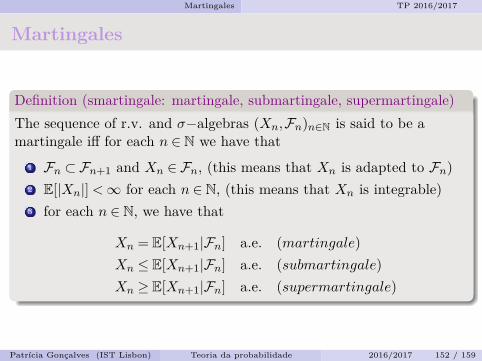
Martingales TP 2016/2017
Martingales
Definition (smartingale: martingale, submartingale, supermartingale)The sequence of r.v. and σ−algebras (Xn,Fn)n∈N is said to be amartingale iff for each n ∈ N we have that
1 Fn ⊂Fn+1 and Xn ∈ Fn, (this means that Xn is adapted to Fn)2 E[|Xn|]<∞ for each n ∈ N, (this means that Xn is integrable)3 for each n ∈ N, we have that
Xn = E[Xn+1|Fn] a.e. (martingale)Xn ≤ E[Xn+1|Fn] a.e. (submartingale)Xn ≥ E[Xn+1|Fn] a.e. (supermartingale)
Patrıcia Goncalves (IST Lisbon) Teoria da probabilidade 2016/2017 152 / 159
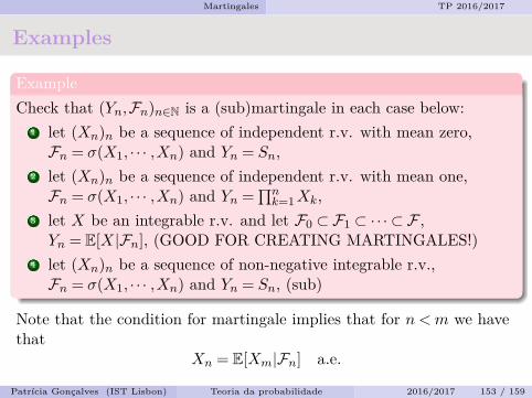
Martingales TP 2016/2017
Examples
ExampleCheck that (Yn,Fn)n∈N is a (sub)martingale in each case below:
1 let (Xn)n be a sequence of independent r.v. with mean zero,Fn = σ(X1, · · · ,Xn) and Yn = Sn,
2 let (Xn)n be a sequence of independent r.v. with mean one,Fn = σ(X1, · · · ,Xn) and Yn =
∏nk=1Xk,
3 let X be an integrable r.v. and let F0 ⊂F1 ⊂ ·· · ⊂ F ,Yn = E[X|Fn], (GOOD FOR CREATING MARTINGALES!)
4 let (Xn)n be a sequence of non-negative integrable r.v.,Fn = σ(X1, · · · ,Xn) and Yn = Sn, (sub)
Note that the condition for martingale implies that for n <m we havethat
Xn = E[Xm|Fn] a.e.
Patrıcia Goncalves (IST Lisbon) Teoria da probabilidade 2016/2017 153 / 159

Martingales TP 2016/2017
Jensen’s inequality
Theorem (Jensen’s inequality)Let (Xn,Fn)n∈N be a submartingal and let ϕ be an increasing convexfunction defined on R. If ϕ(Xn) is integrable for any n, then(ϕ(Xn),Fn)n∈N is also a submartingal.
CorollaryIf (Xn,Fn)n∈N is a submartingal then (X+
n ,Fn)n∈N, (|Xn|,Fn)n∈N,(|Xn|p,Fn)n∈N for 1< p <∞ if Xn ∈ Lp are also submartingales.
Exercise: Prove the theorem.
Patrıcia Goncalves (IST Lisbon) Teoria da probabilidade 2016/2017 154 / 159
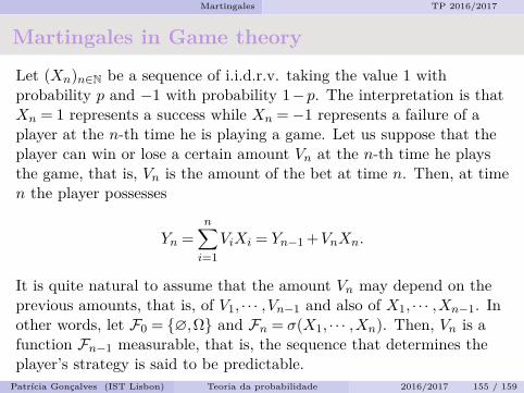
Martingales TP 2016/2017
Martingales in Game theory
Let (Xn)n∈N be a sequence of i.i.d.r.v. taking the value 1 withprobability p and −1 with probability 1−p. The interpretation is thatXn = 1 represents a success while Xn =−1 represents a failure of aplayer at the n-th time he is playing a game. Let us suppose that theplayer can win or lose a certain amount Vn at the n-th time he playsthe game, that is, Vn is the amount of the bet at time n. Then, at timen the player possesses
Yn =n∑i=1
ViXi = Yn−1 +VnXn.
It is quite natural to assume that the amount Vn may depend on theprevious amounts, that is, of V1, · · · ,Vn−1 and also of X1, · · · ,Xn−1. Inother words, let F0 = ∅,Ω and Fn = σ(X1, · · · ,Xn). Then, Vn is afunction Fn−1 measurable, that is, the sequence that determines theplayer’s strategy is said to be predictable.
Patrıcia Goncalves (IST Lisbon) Teoria da probabilidade 2016/2017 155 / 159
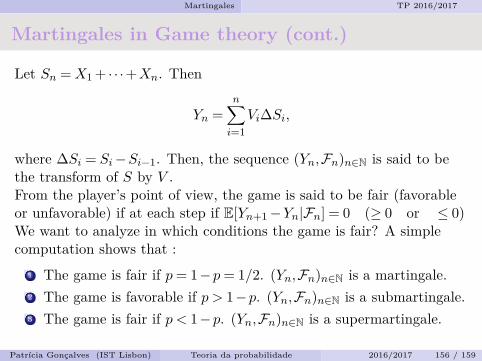
Martingales TP 2016/2017
Martingales in Game theory (cont.)
Let Sn =X1 + · · ·+Xn. Then
Yn =n∑i=1
Vi∆Si,
where ∆Si = Si−Si−1. Then, the sequence (Yn,Fn)n∈N is said to bethe transform of S by V .From the player’s point of view, the game is said to be fair (favorableor unfavorable) if at each step if E[Yn+1−Yn|Fn] = 0 (≥ 0 or ≤ 0)We want to analyze in which conditions the game is fair? A simplecomputation shows that :
1 The game is fair if p= 1−p= 1/2. (Yn,Fn)n∈N is a martingale.2 The game is favorable if p > 1−p. (Yn,Fn)n∈N is a submartingale.3 The game is fair if p < 1−p. (Yn,Fn)n∈N is a supermartingale.
Patrıcia Goncalves (IST Lisbon) Teoria da probabilidade 2016/2017 156 / 159

Martingales TP 2016/2017
Martingales in Game theory (cont.)
Let us now consider another strategy. Take (Vn,Fn−1)n≥1 with V1 = 1and for n≥ 1 we have that Vn = 2n−1 if X1 =−1, · · · ,Xn−1 =−1 and 0otherwise.Under this strategy, a player starts to bet 1 euro and doubles the betin the next play if he had lost or leaves immediately the game in casehe had won.If X1 =−1, · · ·Xn =−1, then the total loss after n plays is∑ni=1 2i−1 = 2n−1.
Therefore, if Xn+1 = 1 thenYn+1 = Yn+Xn+1Vn+1 =−(2n−1) + 2n = 1.Let τ := infn≥ 1 : Yn = 1, that is the first time that Yn = 1. If p= 1
2 ,then the game is fair and
P(τ = n) = P(Yn = 1,Yk 6= 1,∀k = 1, · · · ,n−1) =(1
2)n.
Patrıcia Goncalves (IST Lisbon) Teoria da probabilidade 2016/2017 157 / 159
Martingales TP 2016/2017
Martingales in Game theory (cont.)
From where we conclude that
P(τ <∞) = P(∪n≥1τ = n) =∑n≥1
(12)n
= 1.
Moreover, P(Yτ = 1) = 1 and E[Yτ ] = 1.Therefore, even in a fair game, applying the strategy described above,a player can, in finite time, complete the game with success, that is,increase his capital in one unity: E[Yτ ] = 1> Y0 = 0. In game theorythis type of system - double the bet after a loss and leave the gameimmediately after a win - is called a martingale.We note however that p= 1/2, so that (Yn,Fn)n∈N is a martingale andE[Yn] = E[Y0] = 0 for all n≥ 1. Above the same is not true for arandom time (above we took the random time τ .)
Patrıcia Goncalves (IST Lisbon) Teoria da probabilidade 2016/2017 158 / 159

Martingales TP 2016/2017
Markov time
DefinitionA r.v. τ which takes values in the set 0,1, · · · ,∞ is said to be aMarkov time wrt a σ-algebra Fn if for each n≥ 0 we have thatτ = n ∈ Fn. When P(τ <∞) = 1, the Markov time is said to be astopping time.
If (Xn,Fn)n∈N is a sequence of r.v. and σ-algebras with Fn ∈ Fn+1,and if τ is a Markov time wrt Fn, then we write Xτ =
∑∞n=0Xn1τ=n.
Note that since P(τ <∞) = 1 we have that Xτ = 0 in the set τ =∞.Prove that Xτ is a r.v.
Example (Prove it!)Let (Xn,Fn)n∈N be a martingale (or submartingale) and τ a Markovtime wrt Fn. Then the stopping process Xτ = (Xn∧τ ,Fn) is also amartingale (or submartingale).
Patrıcia Goncalves (IST Lisbon) Teoria da probabilidade 2016/2017 159 / 159