Techniques of Mathematical Modelling

Specimen fhs questions.

Warning: these are rather longer than actual fhs questions would be. In parts theyare also somewhat harder.

1. Explain what is meant by a conservation law and a constitutive law in a mathe-matical model. A certain substance has a density φ of a certain quantity, whichmoves with a flux f . Write down an integral conservation law for the quantityof the substance in an arbitrary volume V , and hence deduce carefully that φsatisfies the partial differential equation

∂φ

∂t+ ∇.f = 0.

The density of cars on a certain one lane highway is ρ (with units of cars perunit length), and the speed v of the cars is measured as a function of the density,

v = v0

(1− ρ

ρ0

)2

.

Give a physical interpretation of the quantities v0 and ρ0, and explain why thisrelation is intuitively sensible.

Write down an equation governing the traffic density, using the above expressionfor car speed, and by choosing suitable non-dimensional variables, show thatthe model can be written in the dimensionless form

∂ρ

∂t+∂q

∂x= 0,

where q = ρ(1− ρ)2, and x represents dimensionless distance along the road.

A line of cars of initial (dimensionless) density ρ0(x) moves along a road −∞ <x <∞, and is governed by the preceding equation. Consider the three situationsin which ρ0(x) is monotonic, with ρ→ ρ− as x→ −∞ and ρ→ ρ+ as x→∞,where (i) ρ− < 1

3< ρ+ < 2

3, (ii) 2

3> ρ− > 1

3> ρ+, (iii) 1

3< ρ− < 2

3< ρ+.

Explain qualitatively, using diagrams, what happens in each case. In particular,describe in which situation(s) a shock forms, and give an expression for theresulting shock speed(s). [An exact solution is not required.]

1

2. Explain what is meant by a regular perturbation and by a singular perturbationfor an algebraic equation and for an ordinary differential equation. [It may beuseful to give illustrative examples.]

The quantity x satisfies the algebraic equation

x4 − εx− 1 = 0.

Suppose that ε ¿ 1. Find approximate expressions, correct to terms of O(ε),for each of the four solutions of the equation.

Now suppose ε À 1. Show that an approximate solution cannot immediatelybe found, but that by a suitable rescaling of the equation (which you shouldfind), it can be written in the form

X4 −X − δ = 0,

where δ = ε−4/3 ¿ 1.

Hence find leading order (non-zero) approximations for all four of the solutions.

Find a more accurate approximation to the smallest root in this case.

2

3. A nonlinear damped pendulum satisfies the equation

lθ + kθ + g sin θ = 0.

Explain the meaning of the terms in this equation, and how it is derived.

Suppose that θ = 0, θ = ω0 at t = 0. By suitably non-dimensionalising theequation, show that the model can be written in the form

θ + θ + ε sin θ = 0,

θ(0) = 0, θ = µ,

and give the definitions of ε and µ.

The pendulum is suspended in a bath of liquid (e. g., water). Why might thisbe consistent with a value of ε¿ 1?

Assume now that ε ¿ 1 and that µ = O(1). Find an approximate solution inthis case, and show that θ → µ for large t.

By rescaling t = τ/ε, find an approximate equation satisfied by θ over thislonger time scale, and explain why a suitable initial condition for θ as τ → 0 isθ ≈ µ.

Hence show that for τ ≥ O(1),

θ ≈ 2 tan−1[e−τ tan

µ

2

].

Do these results accord with your expectation?

3

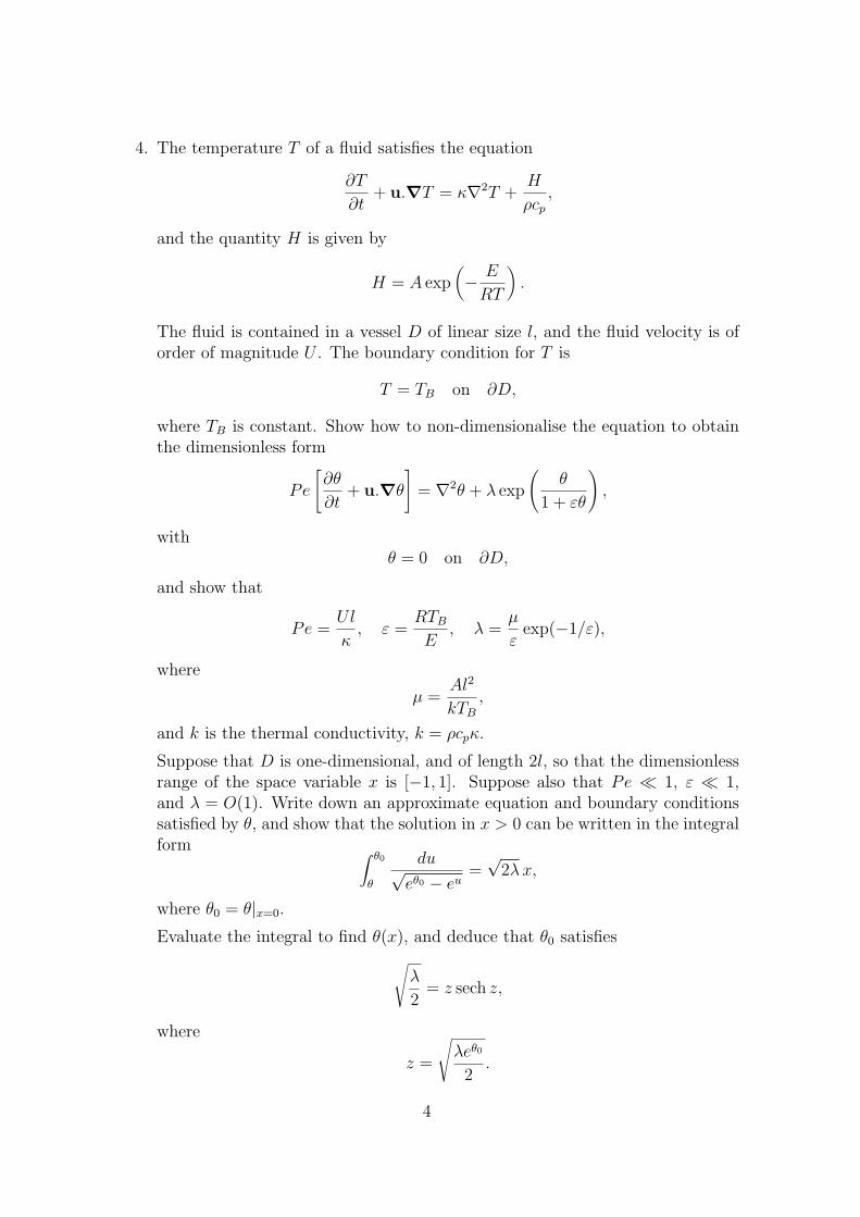
4. The temperature T of a fluid satisfies the equation

∂T

∂t+ u.∇T = κ∇2T +

H

ρcp,

and the quantity H is given by

H = A exp(− E

RT

).

The fluid is contained in a vessel D of linear size l, and the fluid velocity is oforder of magnitude U . The boundary condition for T is

T = TB on ∂D,

where TB is constant. Show how to non-dimensionalise the equation to obtainthe dimensionless form

Pe

[∂θ

∂t+ u.∇θ

]= ∇2θ + λ exp

(θ

1 + εθ

),

withθ = 0 on ∂D,

and show that

Pe =Ul

κ, ε =

RTB

E, λ =

µ

εexp(−1/ε),

where

µ =Al2

kTB

,

and k is the thermal conductivity, k = ρcpκ.

Suppose that D is one-dimensional, and of length 2l, so that the dimensionlessrange of the space variable x is [−1, 1]. Suppose also that Pe ¿ 1, ε ¿ 1,and λ = O(1). Write down an approximate equation and boundary conditionssatisfied by θ, and show that the solution in x > 0 can be written in the integralform ∫ θ0

θ

du√eθ0 − eu

=√

2λx,

where θ0 = θ|x=0.

Evaluate the integral to find θ(x), and deduce that θ0 satisfies

√λ

2= z sech z,

where

z =

√λeθ0

2.

4

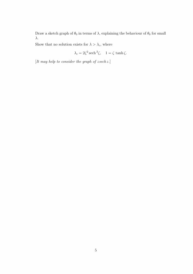
Draw a sketch graph of θ0 in terms of λ, explaining the behaviour of θ0 for smallλ.

Show that no solution exists for λ > λc, where

λc = 2ζ2 sech 2ζ, 1 = ζ tanh ζ.

[It may help to consider the graph of zsech z.]

5

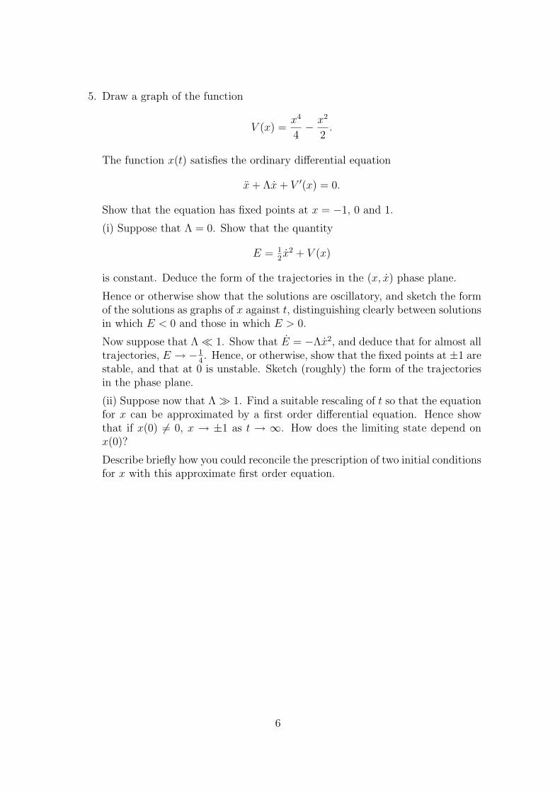
5. Draw a graph of the function

V (x) =x4

4− x2

2.

The function x(t) satisfies the ordinary differential equation

x+ Λx+ V ′(x) = 0.

Show that the equation has fixed points at x = −1, 0 and 1.

(i) Suppose that Λ = 0. Show that the quantity

E = 12x2 + V (x)

is constant. Deduce the form of the trajectories in the (x, x) phase plane.

Hence or otherwise show that the solutions are oscillatory, and sketch the formof the solutions as graphs of x against t, distinguishing clearly between solutionsin which E < 0 and those in which E > 0.

Now suppose that Λ ¿ 1. Show that E = −Λx2, and deduce that for almost alltrajectories, E → −1

4. Hence, or otherwise, show that the fixed points at ±1 are

stable, and that at 0 is unstable. Sketch (roughly) the form of the trajectoriesin the phase plane.

(ii) Suppose now that Λ À 1. Find a suitable rescaling of t so that the equationfor x can be approximated by a first order differential equation. Hence showthat if x(0) 6= 0, x → ±1 as t → ∞. How does the limiting state depend onx(0)?

Describe briefly how you could reconcile the prescription of two initial conditionsfor x with this approximate first order equation.

6

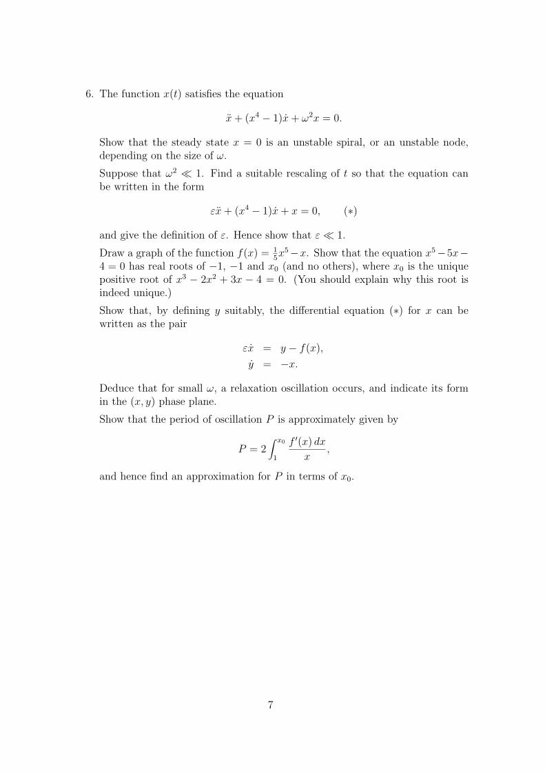
6. The function x(t) satisfies the equation

x+ (x4 − 1)x+ ω2x = 0.

Show that the steady state x = 0 is an unstable spiral, or an unstable node,depending on the size of ω.

Suppose that ω2 ¿ 1. Find a suitable rescaling of t so that the equation canbe written in the form

εx+ (x4 − 1)x+ x = 0, (∗)

and give the definition of ε. Hence show that ε¿ 1.

Draw a graph of the function f(x) = 15x5−x. Show that the equation x5−5x−

4 = 0 has real roots of −1, −1 and x0 (and no others), where x0 is the uniquepositive root of x3 − 2x2 + 3x − 4 = 0. (You should explain why this root isindeed unique.)

Show that, by defining y suitably, the differential equation (∗) for x can bewritten as the pair

εx = y − f(x),

y = −x.

Deduce that for small ω, a relaxation oscillation occurs, and indicate its formin the (x, y) phase plane.

Show that the period of oscillation P is approximately given by

P = 2∫ x0

1

f ′(x) dxx

,

and hence find an approximation for P in terms of x0.

7

7. Describe what is meant by a boundary layer approximation to the solution of adifferential equation.

Describe, giving brief reasons, where you expect the boundary layers to belocated for the solutions of the boundary value problem

εy′′ + a(x)y′ + b(x)y = 0, y(0) = 0, y(1) = 1,

if ε¿ 1 and (i) a(x) > 0; (ii) a(x) < 0.

Find a leading order approximation (including boundary layers, where neces-sary) to the solution of the boundary value problem

εy′′ + (1 + x)y′ + xy = 0, y(0) = 0, y(1) = 2.

Hence show that, approximately,

y′(0) =e

ε.

8

8. Suppose that

X = A(t)X, (∗)

where X ∈ Rn and A is a 2π–perodic n×n matrix, whose elements are contin-uous.

Define what is meant by the fundamental matrix Φ(t), and use it to show thatthe solution of (∗) satisfying X = X0 at t = 0 is given by

X = Φ(t)X0.

Suppose that W = det Φ; show that

W = (trA)W,

and deduce that W is never zero.

Deduce that the monodromy matrix M = Φ(2π) has no zero eigenvalues.

Suppose the (distinct) eigenvalues of M are exp (2πλs), s = 1, 2 . . . n, and thatΛ is the diagonal matrix diag (λs).

If Ψ is the matrix exp(tΛ), show that

Ψ(2π) = diag [exp(2πλs)] .

Suppose now that the constant matrix P satisfies P−1MP = Ψ(2π). Show thatPΨ(2π) = Φ(2π)P , and deduce that the matrix B = ΦPΨ−1P−1 is 2π–periodic.

Show how this can be used to prove Floquet’s theorem, that there is a 2π–periodic matrix B(t) such that X = BY , and

Y = CY,

where C is a constant matrix, which you should find.

Explain how the eigenvalues of C are related to those of M .

9

9. (i) The function u(x, t) satisfies the heat equation

ut = uxx

on 0 < x <∞, together with the initial condition

u = 0 at t = 0,

and the boundary conditions

u = 1 at x = 0,

u→ 0 as x→∞.

Find a similarity solution for u.

(ii) Suppose now that u(x, t) satisfies

ut = (uux)x in 0 < x <∞,

with the same initial and boundary conditions as above.

Show that a similarity solution in the form u = f(η), η =x

ctαcan be found if

α is chosen appropriately, and show that if also c takes a certain value, then fsatisfies the equation

(ff ′)′ + 2ηf ′ = 0.

Write down the boundary conditions for f .

Suppose now that f > 0 for all finite η, and assume that ηf → 0 as η → ∞.By integrating the equation for f , show that f satisfies

f ′ = −2η − 2∫∞η f(ξ) dξ

f,

and deduce thatf < 1− η2

in this case.

Hence show that in fact f must reach zero at some finite value η0. Can thissame argument be used to show that η0 < 1?

10

10. Jensen’s inequality states that

f[∫

Ωg(x) dω

]≤

∫

Ωf [g(x)] dω,

if f is convex, i. e., f ′′ > 0, and the spatial domain Ω has unit measure, i. e.,∫

Ωdω = 1.

The function u satisfies

ut = ∇2u+ λf(u) in Ω,

u = 0 for x ∈ ∂Ω, u = 0 at t = 0,

where Ω is a bounded domain, λ > 0 and f is a positive convex function foru ≥ 0. Assume that u ≥ 0 for t ≥ 0.

Assume that the principal eigenfunction φ and the corresponding eigenvalue µof Helmholtz’s equation

∇2φ+ µφ = 0

satisfy φ > 0 and

µ = minφ

∫

Ω|∇ψ|2 dV

∫

Ω|ψ|2 dV

.

Using the definitions

dω =φ dV∫

Ωφ dV

andv =

∫

Ωu dω,

use Jensen’s inequality to show that

v ≥ −µv + λf(v),

where v = dv/dt.

Suppose now that w(t) satisfies the equation

w = −µw + λf(w), w(0) = 0,

and that f(w) > 0, f ′(w) > 0 for all w ≥ 0. By writing the solution asa quadrature in the form t = I(w), show that if λ is sufficiently large thatλf(w)− µw is positive for all w ≥ 0, then w →∞ as t→ tc, where

tc = I(∞) =∫ ∞

0

dw

λf(w)− µw,

assuming this integral exists.

Show that I(v) is a monotone increasing function of v, and that v satisfies theinequality I(v) ≥ t. Deduce that v ≥ w, and therefore that u must blow up infinite time.

11

11. A forced pendulum satisfies the equation

lθ + kθ + g sin θ = a sinαt.

By scaling the equation suitably, show that this can be written in the dimen-sionless form

θ + βθ + sin θ = ε sinωt,

and give the definitions of β, ε and ω.

Suppose that ε¿ 1 and θ ¿ 1. Find an approximate linear equation for θ andobtain its (particular) solution if β = 0. Plot the amplitude A = max |θ| as afunction of the driving frequency ω.

Now suppose β 6= 0 (but is still small). Find the solution (ignoring the transient)and show that its amplitude A is given by

A =ε

|1− ω2 + iβω| .

Next consider the oscillator when β = 0 and ε = 0. Find a first integral of themotion, plot the trajectories in the (θ, θ) phase plane, and hence deduce thatthe period of oscillation P is given by

P = 4∫ A

0

du√2[E − (1− cosu)]1/2

,

where A is the amplitude of the oscillation, and

E(A) = 1− cosA.

Hence show that the frequency of the undamped, unforced pendulum is givenby

Ω(A) =π

√2∫ A

0

du

[cosu− cosA]1/2

.

Show that Ω → 1 as A→ 0.

Suppose that when β 6= 0 and ε 6= 0, the amplitude of oscillation is related tothe forcing frequency by

A = R[Ω(A)],

whereR(Ω) =

ε

|Ω2 − ω2 + iβω| .

Assume that Ω(A) = 1− 18A2; write down an expression for the inverse function

A = I(Ω).

By consideration of the intersection of the graphs of I(Ω) and R(Ω), show that,for sufficiently small ε and β, there can be one, three, or exceptionally twovalues of Ω (and thus A) for given ω. Draw a graph of the amplitude A interms of ω.

12

12. The size of courgette plants in my garden is measured by the leaf area L. Therate of growth of the plants is proportional to leaf area, and also to receivedsunlight, which is itself proportional to leaf area. Additionally, the plants grow

to a maximum size. Explain why a growth rate for L of gL2(1− L

L0

)represents

these assumptions.

Slugs consume courgette leaves at a rate rS, where S is slug density, and Iplant out seedlings at a rate p (leaf area per unit time). Explain why a modelequation for leaf area can be assumed to be

L = p− rS + gL2(1− L

L0

),

where L = dL/dt.

Assume to begin with that the slug density S is constant. Non-dimensionalisethe equation to obtain the dimensionless model

l = 1− ρ+ γl2 (1− l) ,

and define the parameters ρ and γ.

Show that if ρ < 1, the plants grow to a healthy size.

Show that if ρ > 1 +4γ

27, I cannot grow courgettes.

Show that if 1 < ρ < 1 +4γ

27, there is a threshold value lc such that if l > lc,

plants will thrive, but if l < lc, plants will die out.

Draw a graph of the steady state l versus ρ, and show that this response diagramindicates hysteresis as ρ varies. Indicate where l > 0 and l < 0 on the diagram,and thus determine the stability of the steady state(s).

In reality, the slug consumption rate depends on leaf area. Suppose now that

r =r0L

L+ Lc

.

Write down the corresponding form of the dimensionless model in this case.Suppose that l0 = Lc/L0 is small. Draw a response diagram of steady statel versus ρ0 = r0S/p in this case, indicating carefully how this diagram differsfrom the previous one.

Show that the diagram again displays hysteresis, and that there are two valuesρ− and ρ+ such that for ρ− < ρ0 < ρ+, there are three possible steady state

values of l, only two of which are stable. Show that ρ− → 1 and ρ+ → 1 +4γ

27as l0 → 0, and that the corresponding values l− → 0 and l+ → 2/3.

Slugs are attracted towards foliage at a rate proportional to leaf area, and Ikill them at a rate proportional to their number. Explain why a suitable modelequation for slug density is

S = aL− bS,

13

and show that by suitable choice of the slug density scale, the dimensionlessslug model can be written in the form

s = l − µs,

and give the definition of µ.

Hence show that for small killing rate or high planting rate, a stable state occursin which slugs win, but for high killing rate or low planting rate, the plants win.Show also that for intermediary rates, oscillations are possible.

14

13. The variables x and y satisfy the ordinary differential equations

x = f(x, y),

y = g(x, y),

where x = dx/dt, y = dy/dt, and t denotes time. Suppose (x0, y0) is a fixed pointof these equations. Describe how the stability of the fixed point is determinedby the trace T and determinant D of the community matrix

M =

(fx fy

gx gy

),

and indicate on a diagram in which regions of (T,D) space the fixed point is asaddle, a node, or a spiral. Give a necessary and sufficient condition on T andD for (x0, y0) to be stable.

The functions G(x) and H(x) are defined for positive x by

G(x) = x2e−x, H(x) = βe−2x,

where β > 0. Show that the equation G(x) = H(x) has a unique positiveroot. If this root is denoted by x0(β), show (for example, graphically) that x0

increases with β, and that x0 → 0 as β → 0 and x0 →∞ as β →∞.

Now suppose that in the differential equations for x and y,

f(x, y) = y −G(x), g(x, y) = H(x)− y,

and suppose that x and y are initially non-negative. Show that x and y remainpositive for t > 0.

Show that there is a unique fixed point P at (x0, H(x0)) in the positive quadrant.Draw the nullclines in the phase plane, indicating on your diagram the directionof trajectories in the four regions of the positive quadrant delineated by thenullclines.

Show that the trace T and the determinant D of the community matrix at thefixed point P are given by

T = −G′(x0)− 1, D = G′ −H ′,

and deduce that D > 0 for all positive values of β.

Derive an expression for −G′(x), and show that it has a maximum at x = xM =2+

√2. Assuming that −G′(xM) < 1, deduce (explaining why) that P is stable

for all positive values of β.

15

14. The Fisher equation is given by

ut = ru[1− u

K

]+ Duxx.

If r, K and D are constant, show how to non-dimensionalise the equation tothe form

ut = u [1− u] + uxx.

If, initially, u = 0 except on a finite interval where it is small and positive,explain using diagrams how you would expect the solution to evolve. Verify yourdescription by seeking travelling wave solutions of the form u = f(ξ), ξ = x−ct,and write down the resulting equation and boundary conditions which f mustsatisfy, assuming that c > 0. How should the boundary conditions be modifiedif c < 0?

By examining the solutions in a suitable phase plane, show that a travellingwave in which u > 0 is positive is possible if c ≥ 2. What happens if c < 2?

Sketch the form of the wave as a function of ξ. If, instead, D = D0u, what formwould you expect a travelling wave to take, assuming such a wave exists?

16

15. The function u(x, t) satisfies the equation

ut + uux = −βu,

with initial conditions

u = u0(x) on −∞ < x <∞,

and u0 > 0, u→ 0 as x→ ±∞.

Use the method of characteristics to derive the solution in the parametric form

u = u0(s)e−βt,

x = s+u0(s)

(1− e−βt

)

β.

Assume that β > 0 and that t ≥ 0. By first writing u = F (x, t, u), or otherwise,find an expression for ux, and hence show that a shock will develop if max |u′0| >β.

Suppose that u0(s) = α(1 − |s|) for s ∈ (−1, 1), and u0 = 0 otherwise. If0 < α < β, show that characteristics do not intersect, and deduce that u = 0for |x| > 1. By considering the characteristics from 0 < s < 1, show also that

u =αβ(1− x)e−βt

β − α(1− e−βt)

forα((1− e−βt)

β< x < 1. Write down a corresponding expression for u in

0 < x <α((1− e−βt)

β. Draw the characteristic diagram for the solution.

17

16. The function u(x, t) satisfies the equation

ut + u2ux = εuxx

on (−∞,∞), where ε ¿ 1. At t = 0, u = u0(x), where u0 is positive and

u0(±∞) = 0. Show that∫ ∞

−∞u dx is conserved in time.

If the diffusion term is neglected, use the method of characteristics to solve theequation, and hence derive an expression for ux as a function of x, t and u.Use this to show that a shock will form for t > 0 if u′0 < 0, and this occurs at

t = minu′0<0

1

2u0|u′0|.

Suppose u0(x) = V (1 − |x|) for |x| < 1, u0 = 0 otherwise, where V > 0. Show

that a shock first forms when t =1

2V 2, at the point x = 1

2. Draw the shape of

u as a function of x at this time.

For time t >1

2V 2, a shock propagates forwards at a position x = X(t). If the

value of u behind the front is U(t), show that, for large enough t,

tU2 +U

V− 1−X = 0,

and that (also for large enough t)

X = 13U2.

Deduce that for large t and X,

U ≈(X

t

)1/2

,

and hence thatX ≈ at1/3,

and use the value of the conserved integral∫ ∞

−∞u dx to show that

a =(

3V

2

)2/3

.

If ε is small but non-zero, show that a shock structure consistent with thisdescription is possible, by writing x = X+εξ, and solving the resulting approx-imate equation for u with the boundary conditions u→ U as ξ → −∞, u→ 0as ξ →∞.

18

17. A model of snow melt run off from a snow pack is described by the equations

φ∂S

∂t+∂u

∂z= 0,

u = −k(S)

µ

[∂p

∂z− ρg

],

pa − p = pc(S),

where z measures distance downwards from the surface of the snowpack, andS ∈ (0, 1) is the relative water saturation (S = 1 represents total saturation,S = 0 represents complete dryness).

Show that the equations can be reduced to a single equation for S of the form

φ∂S

∂t=

∂

∂z

[D(S)

∂S

∂z−K(S)

],

and give the definitions of the hydraulic diffusivity D(S) and hydraulic conduc-tivity K(S).

If k(S) = k0kr(S) and pc(S) = p0f(S), where kr and f are dimensionless andof O(1), show that a dimensionless model can be written in the form

∂S

∂t= −∂u

∂z=

∂

∂z

[D(S)

∂S

∂z− εkr(S)

],

where nowD(S) = −kr(S)f ′(S),

u is the dimensionless flux, and

ε =ρgd

p0

,

d being a suitable length scale.

Assume now that kr(S) = S2 and f(S) = ln(1/S). Find the form of the equationfor S in this case.

An initially dry snowpack (i. e., with S = 0) of depth d begins to melt, so thatthe dimensional surface flux for t > 0 is u|z=0 = q. Show that the corresponding

dimensionless surface flux is q∗ =µdq

k0p0

.

Supposing that ε ¿ 1, show that a similarity solution in the form S = tαg(η),η = z/tβ, which describes the advance of the wetting front into the snowpackcan be found, if

(gg′)′ = 13g − 2

3ηg′,

andgg′ = −q∗ on η = 0.

19

Explain briefly why for this model there is a finite wetting front, i. e., g = 0 atη = η0.

Show that∫ η0

0g dη = q∗.

Show that

g′ = −23η −

∫ η0

ηg dη

g,

and deduce that g′ < −23η.

If g = g0 at η = 0, show that g < g0 − 13η2, and deduce that g0 >

13η2

0. Show

also that the integral constraint on g implies g0 >19η2

0 +q∗

η0

.

By graphical means, show that these two inequalities together imply that g0 >(3q∗2/4)1/3.

Show that the dimensionless breakthrough time (when the wetting front reaches

the base of the snow pack) is tB = 1/η3/20 , and the dimensionless ponding time

(when the surface saturation reaches S = 1) is tS = 1/g30. By means of the

above inequalities, show that (tB/tS)1/3 > (g30/3)1/4, and hence deduce that

tB > tS if q∗ > 2.

20

18. The function u(x, t) satisfies the nonlinear diffusion equation

ut = [(D + u)ux]x on 0 < x <∞,

where D is a non-negative constant, together with the boundary conditionsu = 1 at x = 0, u → 0 as x → ∞, and the initial condition u = 0 at t = 0.Show that a similarity solution in the form u = f(η), η = x/ctβ, can be found,where for suitable constants c and β, f satisfies

[(D + f)f ′]′ + 2ηf ′ = 0. (1)

Write down the boundary conditions satisfied by f .

Suppose that f(η) is any analytic function satisfying an equation of the form

f ′′ = φ2,1(η, f, f′)f ′,

where φ2,1(η, f, g) has derivatives of all orders with respect to f and g. Showby induction that

f (n) = φn,1(η, f, f′)f ′ + . . .+ φn,n−1(η, f, f

′)f (n−1),

and deduce that if f ′ = 0 at a point, then f ′ ≡ 0.

Hence show that the solution of equation (1) satisfying the boundary conditionsyou have prescribed must be monotonically decreasing.

Deduce from this that if D > 0, then f > 0 for all finite η. Why does thisconclusion not apply if D = 0?

Show, contrarily, that if D = 0, then ff ′ < −2ηf , and deduce that f mustreach 0 at a finite value of η = η0, and that in fact η0 < 1.

21

19. A small drop of fluid of depth h sits on a horizontal plane. The equation ofconservation of mass can be written in the form

ht + ∇.q = 0,

where q denotes the horizontal fluid flux (i. e., the integral over the depth of thehorizontal velocity). Assume that the horizontal fluid flux, q, can be approxi-mated as

q = −ρgh3

3µ∇h,

where ρ is density, g is gravity, and µ is the viscosity.

Hence derive the evolution equation

ht =ρg

3µ∇.[h3∇h],

and show that it can be written in the dimensionless form

ht = ∇.[h3∇h].

A lava dome is modelled by a shallow two-dimensional fluid flow of dimensionlessdepth h(x, t) satisfying the above equation in one space variable x. The eruptionrate is modelled by a prescribed dimensionless flux q = 1 at x = 0. Restrictingattention to the dome shape in x > 0, show that it may be modelled by theequation

ht =[h3hx

]x

in x > 0,

withh3hx = −1 on x = 0, h→ 0 as x→∞.

Look for a similarity solution of the form h = tαf(η), η = x/tβ to the aboveequations and boundary conditions for a suitable choice of α and β, and showthat f satisfies (

f 3f ′)′

+ 45(ηf)′ = f,

with (f 3f ′

)′= −1 at η = 0, f(∞) = 0.

If f first reaches zero when η = η0 (which may be infinite) (thus f > 0 forη < η0), show that

f 3f ′ = −45ηf −

∫ η0

ηf dη.

Deduce that f ′ < 0, and that

f 2f ′ < −45η

while η < η0. Hence show that η0 is in fact finite, and that

η0 <

√5f(0)3

6.

22