TD() and the Proximal Algorithmdimitrib/Proximal_TD_Slides_NIPS.pdf · TD( ) and the Proximal...

TD(λ) and the Proximal Algorithm

Dimitri P. Bertsekas

Laboratory for Information and Decision SystemsMassachusetts Institute of Technology

Optimization Methods Workshop

NIPS 2017

Bertsekas (M.I.T.) TD(λ) and the Proximal Algorithm 1 / 30

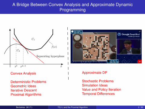
A Bridge Between Convex Analysis and Approximate DynamicProgramming

Convex Analysis

Deterministic ProblemsGeometric IdeasIterative DescentProximal Algorithms

Approximate DP

Stochastic ProblemsSimulation IdeasValue and Policy IterationTemporal Differences

4

Polyhedral Convexity Template

x0 x1 x2 x3 x4 f(x) X x

f(x0) + (x − x0)′g0

f(x1) + (x − x1)′g1

αx + (1 − α)y, 0 ≤ α ≤ 1

< 90◦

Level set!x | f(x) ≤ f∗ + αc2/2

"Optimal solution set x0

X

xk − αkgk

xk+1 = PX(xk − αkgk)

x∗

xk

1

4


x0 x1 x2 x3 x4 f(x) X x

f(x0) + (x − x0)′g0

f(x1) + (x − x1)′g1

αx + (1 − α)y, 0 ≤ α ≤ 1

< 90◦

Level set!x | f(x) ≤ f∗ + αc2/2

"Optimal solution set x0

X

xk − αkgk

xk+1 = PX(xk − αkgk)

x∗

xk

1

C1 C2 H Normal xk�xk+1

ck xk xk+1

�k � 12ck kx � xkk2 �k f(xk)

Constraint set X x Ha Hb a w b sa sb a b yk = (Xk)�1xk yk+1

yk = (1, 1, 1)

(a) (b) xk xk+2 xk+3 xkrf(xk) xk+1 = xk + dk xk � ↵kDkrf(xk)

↵02x = b2 ↵0

1x = b1 a2 a1 (µ1 < 0) (µ2 > 0) �µ2a2 �µ1a1

{x | Ax = b, x � 0} x⇤ {x | Ax = b} {y | AXk = b}

Feasible directions at x d z � x⇤ x � x⇤ x⇤ = 0 x x⇤ � srf(x⇤)

Level sets of f �(t) = max{0, t} t �(t,�, c) x0ref x1

exp x3ref x4 =

x1ref x5 = x3

ref x0 x1 x2 x3

Origin of Destination of OD Pair w rw x1 x2 x3 x4 rf(x) xk+2 xk+3

xk+2 � sk+2rf(xk+2) xk+1 � sk+1rf(xk+1) xk+1 = xk � skrf(xk)

Constraint set X z � x⇤ x � x⇤ x⇤ = 0 x rf(x⇤) Level sets of f�(t) = max{0, t} t �(t,�, c) x0

ref x1exp x3

ref x4 = x1ref x5 = x3

ref

x0 x1 x2 x3 x4 x⇤ x xk xk�1 xk+1 �1 1 0 �k ↵k x1 x0 x2 X1 X2 rf(x2)

d0 d1 y2 ⇠0 ⇠1 ⇠2 x0 x1 x2 x0 x1 d1 = Q�1/2w1 d0 = Q�1/2w0

y0 y1 y2 w0 w1 ⇠0 = �c10d0 d1 = ⇠1 + c10d0 d2 = ⇠2 + c20d0 + c21d1

xi xref xmax xmin xnew xexp x xnew = xref (a) (b) (c) (d)

� �1 �2 �n�1 �nPn

i=1 ⇠i�i1�

�1+�n��1�n

1�

�1+�n�Pn

i=1⇠i�i

�1�n

�(⇠) =1Pn

i=1 ⇠i�i (⇠) =

nX

i=1

⇠i�i

1


ck xk xk+1



yk = (1, 1, 1)


↵02x = b2 ↵0

1x = b1 a2 a1 (µ1 < 0) (µ2 > 0) �µ2a2 �µ1a1




exp x3ref x4 =

x1ref x5 = x3

ref x0 x1 x2 x3




ref x1exp x3


ref


d0 d1 y2 ⇠0 ⇠1 ⇠2 x0 x1 x2 x0 x1 d1 = Q�1/2w1 d0 = Q�1/2w0



� �1 �2 �n�1 �nPn

i=1 ⇠i�i1�

�1+�n��1�n

1�

�1+�n�Pn

i=1⇠i�i

�1�n

�(⇠) =1Pn

i=1 ⇠i�i (⇠) =

nX

i=1

⇠i�i

1


ck xk xk+1



yk = (1, 1, 1)


↵02x = b2 ↵0

1x = b1 a2 a1 (µ1 < 0) (µ2 > 0) �µ2a2 �µ1a1




exp x3ref x4 =

x1ref x5 = x3

ref x0 x1 x2 x3




ref x1exp x3


ref


d0 d1 y2 ⇠0 ⇠1 ⇠2 x0 x1 x2 x0 x1 d1 = Q�1/2w1 d0 = Q�1/2w0



� �1 �2 �n�1 �nPn

i=1 ⇠i�i1�

�1+�n��1�n

1�

�1+�n�Pn

i=1⇠i�i

�1�n

�(⇠) =1Pn

i=1 ⇠i�i (⇠) =

nX

i=1

⇠i�i

1


ck xk xk+1



yk = (1, 1, 1)


↵02x = b2 ↵0

1x = b1 a2 a1 (µ1 < 0) (µ2 > 0) �µ2a2 �µ1a1




exp x3ref x4 =

x1ref x5 = x3

ref x0 x1 x2 x3




ref x1exp x3


ref


d0 d1 y2 ⇠0 ⇠1 ⇠2 x0 x1 x2 x0 x1 d1 = Q�1/2w1 d0 = Q�1/2w0



� �1 �2 �n�1 �nPn

i=1 ⇠i�i1�

�1+�n��1�n

1�

�1+�n�Pn

i=1⇠i�i

�1�n

�(⇠) =1Pn

i=1 ⇠i�i (⇠) =

nX

i=1

⇠i�i

1


ck xk xk+1


Separating hyperplane


yk = (1, 1, 1)


↵02x = b2 ↵0

1x = b1 a2 a1 (µ1 < 0) (µ2 > 0) �µ2a2 �µ1a1




exp x3ref x4 =

x1ref x5 = x3

ref x0 x1 x2 x3




ref x1exp x3


ref


d0 d1 y2 ⇠0 ⇠1 ⇠2 x0 x1 x2 x0 x1 d1 = Q�1/2w1 d0 = Q�1/2w0



� �1 �2 �n�1 �nPn

i=1 ⇠i�i1�

�1+�n��1�n

1�

�1+�n�Pn

i=1⇠i�i

�1�n

�(⇠) =1Pn

i=1 ⇠i�i (⇠) =

nX

i=1

⇠i�i

1


Fixed Point Problem Formulation

Problem: Solve x = T (x)

We assume that T : <n 7→ <n has a unique fixed point and is nonexpansive,∥∥T (x1)− T (x2)∥∥ ≤ γ‖x1 − x2‖, ∀ x1, x2 ∈ <n,

where 0 ≤ γ ≤ 1 and ‖ · ‖ is some norm

Special focus for this talk: The linear case

x = Ax + b

where I − A is invertible and A has spectral radius ≤ 1


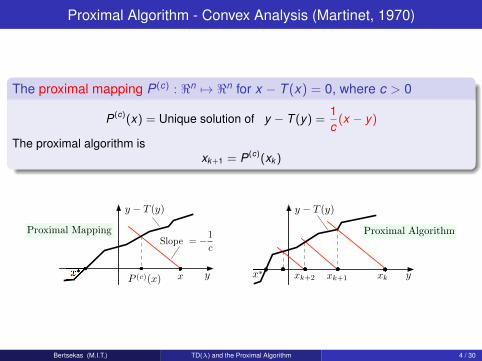
Proximal Algorithm - Convex Analysis (Martinet, 1970)

The proximal mapping P(c) : <n 7→ <n for x − T (x) = 0, where c > 0

P(c)(x) = Unique solution of y − T (y) =1c

(x − y)

The proximal algorithm isxk+1 = P(c)(xk )

x∗ x∗ c v xkk xk+1+1 xk+2d z xP (c)(x)

) y − T (y) ) y − T (y)

) y − ) y −

+2 Slope = −1

c

) Proximal Mapping Proximal Algorithm ) Proximal Mapping Proximal Algorithm


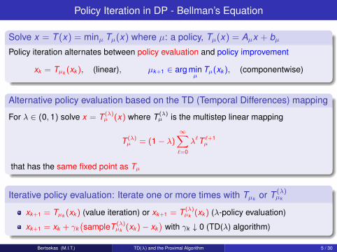
Policy Iteration in DP - Bellman’s Equation

Solve x = T (x) = minµ Tµ(x) where µ: a policy, Tµ(x) = Aµx + bµ

Policy iteration alternates between policy evaluation and policy improvement

xk = Tµk (xk ), (linear), µk+1 ∈ arg minµ

Tµ(xk ), (componentwise)

Alternative policy evaluation based on the TD (Temporal Differences) mapping

For λ ∈ (0, 1) solve x = T (λ)µ (x) where T (λ)

µ is the multistep linear mapping

T (λ)µ = (1− λ)

∞∑`=0

λ`T `+1µ

that has the same fixed point as Tµ

Iterative policy evaluation: Iterate one or more times with Tµk or T (λ)µk

xk+1 = Tµk (xk ) (value iteration) or xk+1 = T (λ)µk (xk ) (λ-policy evaluation)

xk+1 = xk + γk(sampleT (λ)

µk (xk )− xk)

with γk ↓ 0 (TD(λ) algorithm)


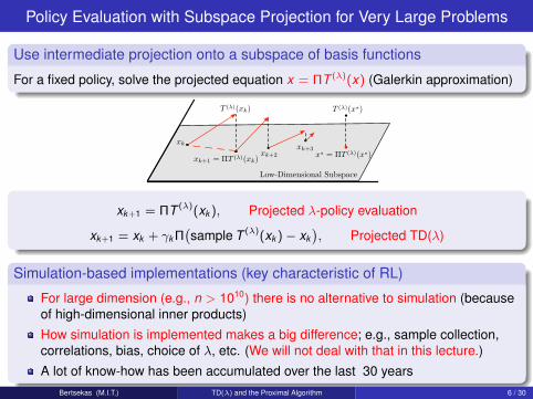
Policy Evaluation with Subspace Projection for Very Large Problems

Use intermediate projection onto a subspace of basis functions

For a fixed policy, solve the projected equation x = ΠT (λ)(x) (Galerkin approximation)

xk

xk+2

xk+3

Extrapolated Forward-Backward Step Low-Dimensional Subspace

xk+1 = ΠT (λ)(xk)

) T (λ)(xk) ) T (λ)(x∗)

) x∗ = ΠT (λ)(x∗)

xk+1 = ΠT (λ)(xk ), Projected λ-policy evaluation

xk+1 = xk + γk Π(sample T (λ)(xk )− xk

), Projected TD(λ)

Simulation-based implementations (key characteristic of RL)

For large dimension (e.g., n > 1010) there is no alternative to simulation (becauseof high-dimensional inner products)

How simulation is implemented makes a big difference; e.g., sample collection,correlations, bias, choice of λ, etc. (We will not deal with that in this lecture.)

A lot of know-how has been accumulated over the last 30 yearsBertsekas (M.I.T.) TD(λ) and the Proximal Algorithm 6 / 30

KEY POINT OF THIS TALKTD(λ) Map for Policy Evaluation ≈ Proximal Map for the Lin. Bellman Eq

T P

T Px

T P (c)

T P (c)

λ =c

c + 1, c =

λ

1 − λ

T (λ)(x) = x + c+1c

(P (c)(x) − x

)

(

J T (x)

)T (λ)(x) = (P (c)T )(x) = (TP (c))(x)

) P (c)(x) = x + λ(T (λ)(x) − x

)

Extrapolation Formula T (λ) = T · P (c) = P (c) · T

T (λ) IS FASTER

TD(λ) IS A STOCHASTIC PROXIMAL ALGORITHM FOR LINEAR FIXED POINTS


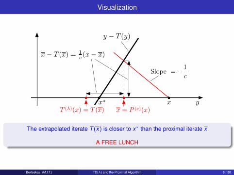
Visualization

4


xk

xk+1

g

fS(s | H0)

x∗

X

Level Sets of f

∂f(x∗)

Significance Levels s − t s + tSpace of Measurement XH0 True Type I Error

1

Pc,f (z) ⌃f(x) 0 slope � c v xk xk+1 xk+2

w pW (·; x) z = g(w) g

⇤k � Dk(x, xk) ⇤k+1 � Dk+1(x, xk+1)

Ty3 x3 Slope = y3

rx(z) = �(cl⇧)(x, z)

rx(µ) � ⌅ µ Z (u, 1)

= Min Common Value w�

= Max Crossing Value q�

Positive Halfspace {x | a⇥x ⇥ b}

a�(C) C C ⇤ S⇤ d z x

Hyperplane {x | a⇥x = b} = {x | a⇥x = a⇥x}

x� x f��x� + (1 � �)x

⇥

x x�

x0 � d x1 x2 x x4 � d x5 � d d

x0 x1 x2 x3

a0 a1 a2 a3

f(z)

z

X 0 u w (µ,⇥) (u, w)µ

⇥

⇥u + w

1

x � T (x) y � T (y) rf(x) P (c)(x) xk xk+1 xk+2

1


1

x � T (x) y � T (y) rf(x) P (c)(x) xk xk+1 xk+2 Slope = �1

c

1

x − T (x) y − T (y) ∇f(x) x − P (c)(x) xk xk+1 xk+2 Slope = −1

c

T (λ)(x) = T (x) x = P (c)(x)

1


c

T (λ)(x) = T (x) x = P (c)(x)

1

xc = ΠP (c)(xc) Bias (→ 0 as c → ∞) E(c)(x) = T (x) P (c)(xc)

x − T (x) = 1c (x − x)

Q(λ) = (Ψ′ΞΦ)−1Ψ′ΞA(λ)Φ d(λ) = (Ψ′ΞΦ)−1Ψ′Ξb(λ) S = {Φr | r ∈ ℜs} x∗ Πx∗ x

xλ = ΠT (xλ) Πx∗ Bias (→ 0 as λ → 1) T (xλ) x Projection ΠxSolution Approximate solution

T (λ)(x) = T (x) x = P (c)(x)


c

T (λ)(x) = T (x) x = P (c)(x)

Extrapolation by a Factor of 2 T (λ) = P (c) · T = T · P (c)

Extrapolation Formula T (λ) = P (c) · T = T · P (c)

Multistep Extrapolation T (λ) = P (c) · T = T · P (c)

1

The extrapolated iterate T (x) is closer to x∗ than the proximal iterate x

A FREE LUNCH


Potential Implications of the TD-Proximal Relation

Benefit to the TD contextClarify the nature of TD(λ) and other TD methods

Bring proximal methodology and insights to bear on exact and approximate DP

Benefit to the proximal contextBring large scale DP/RL methodology to bear on the proximal mainstream

Develop new convex analysis algorithms based on DP/RL ideas


References for this Talk

D. P. Bertsekas, “Proximal Algorithms and Temporal Differences for Large LinearSystems: Extrapolation, Approximation, and Simulation," Report LIDS-P-3205,MIT, Oct. 2016 (rev. Nov. 2017)

Related book references:D. P. Bertsekas, Abstract Dynamic Programming, 2nd Edition, in press

D. P. Bertsekas, Convex Optimization Algorithms, 2015

D. P. Bertsekas and J. N. Tsitsiklis, Neuro-Dynamic Programming, 1996

Related works on Monte Carlo solution methods for linear systems:D. P. Bertsekas and H. Yu, “Projected Equation Methods for Approximate Solutionof Large Linear Systems," J. of Comp. and Applied Mathematics, Vol. 227, 2009

M. Wang and D. P. Bertsekas, “Convergence of Iterative Simulation-BasedMethods for Singular Linear Systems", Stoch. Systems, Vol. 3, 2013

M. Wang and D. P. Bertsekas, “Stabilization of Stochastic Iterative Methods forSingular and Nearly Singular Linear Systems", Math. of Op. Res., Vol. 39, 2013


Outline

1 Acceleration of the Proximal Algorithm for Linear Systems

2 Acceleration of the Proximal Algorithm for Nonlinear Systems

3 Acceleration of Forward-Backward and Proximal Gradient Algorithms

4 Linearized Proximal Algorithms for Nonlinear Systems


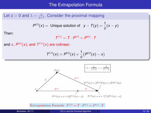
The Extrapolation Formula

Let c > 0 and λ = cc+1 . Consider the proximal mapping


(x − y)

Then:T (λ) = T · P(c) = P(c) · T

and x , P(c)(x), and T (λ)(x) are colinear:

T (λ)(x) = P(c)(x) +1c(P(c)(x)− x

)

T P

T Px

T P (c)

T P (c)

λ =c

c + 1, c =

λ

1 − λ

T (λ)(x) = x + c+1c

(P (c)(x) − x

)

(

J T (x)

)T (λ)(x) = (P (c)T )(x) = (TP (c))(x)

) P (c)(x) = x + λ(T (λ)(x) − x

)

Extrapolation Formula T (λ) = T · P (c) = P (c) · TBertsekas (M.I.T.) TD(λ) and the Proximal Algorithm 13 / 30

Proof outline

Main idea: Express the proximal mapping in terms of a power seriesWe have

P(c)(x) =

(c + 1

cI − A

)−1(b +

1c

x)

and by a series expansion(c + 1

cI − A

)−1

=

(1λ

I − A)−1

= λ(I − λA)−1 = λ

∞∑`=0

(λA)`

Recall that

T (λ)(x) = (1− λ)∞∑`=0

λ`A`+1x +∞∑`=0

λ`A`b

Using these relations and the fact 1c = 1−λ

λ, it follows that

T (λ) = T · P(c) = P(c) · T


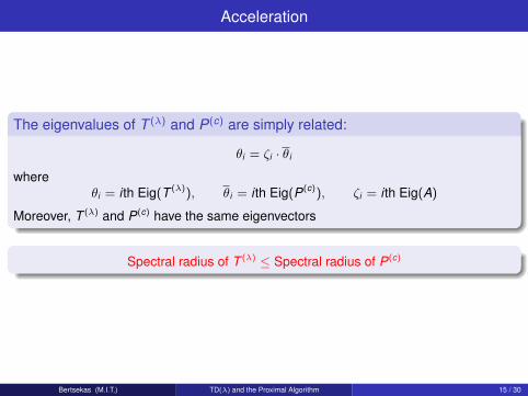
Acceleration

The eigenvalues of T (λ) and P(c) are simply related:

θi = ζi · θi

whereθi = i th Eig(T (λ)), θi = i th Eig(P(c)), ζi = i th Eig(A)

Moreover, T (λ) and P(c) have the same eigenvectors

Spectral radius of T (λ) ≤ Spectral radius of P(c)


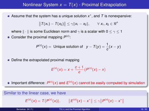
Nonlinear System x = T (x) - Proximal Extrapolation

Assume that the system has a unique solution x∗, and T is nonexpansive:∥∥T (x1)− T (x2)∥∥ ≤ γ‖x1 − x2‖, ∀ x1, x2 ∈ <n

where ‖ · ‖ is some Euclidean norm and γ is a scalar with 0 ≤ γ ≤ 1

Consider the proximal mapping P(c):


(x − y)

Define the extrapolated proximal mapping

E (c)(x) = x +c + 1

c(P(c)(x)− x

)Important difference: P(c)(x) and E (c)(x) cannot be easily computed by simulation

Similar to the linear case, we have

E (c)(x) = T(P(c)(x)

),

∥∥E (c)(x)− x∗∥∥ ≤ γ∥∥P(c)(x)− x∗

∥∥Bertsekas (M.I.T.) TD(λ) and the Proximal Algorithm 18 / 30

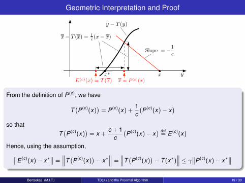
Geometric Interpretation and Proof

x∗ d z x

) y − T (y)

) y −

+2 Slope = −1

c

x = P (c)(x)) E(c)(x) = T (x)

x − T (x) = 1c (x − x)

From the definition of P(c), we have

T(P(c)(x)

)= P(c)(x) +

1c(P(c)(x)− x

)so that

T(P(c)(x)

)= x +

c + 1c(P(c)(x)− x

) def= E (c)(x)

Hence, using the assumption,∥∥E (c)(x)− x∗∥∥ =

∥∥∥T(P(c)(x)

)− x∗

∥∥∥ =∥∥∥T(P(c)(x)

)− T (x∗)

∥∥∥ ≤ γ∥∥P(c)(x)− x∗∥∥


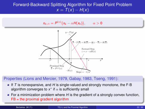
Forward-Backward Splitting Algorithm for Fixed Point Problemx = T (x)− H(x)

xk+1 = P(α)(xk − αH(xk )), α > 0

≥ π/2 Pc,f(x)−x λ∗−cv∗ = (N1·N2)(λ∗−cv∗) 0 λ∗ N2(λ∗−cv∗) v∗ ∂h(x) x −∇f(x)

Slope Optimal dual proximal solution Optimal primal

x∗ = Pc,f (x∗) Nc,f(x)− x∗ Nc,f(x) X∗ x− x∗ < π/2 (N1 · N2)(yk) N2(yk)

xk−1 xk+1 yk yk+1 xk+2 ∇f(xk+1) yk − α∇f(yk) X

yk = xk − γk∇f(xk) yk = xk + βk(xk − xk−1)

x0 = x−1 x1 = y1 y2 x2 = x∗ xk+2 ∇f(xk+1)

y2 = x1 − α1∇f(x1) x2 = y2 + β2(xk − xk−1)

Gradient Projection Step Extrapolation StepOptimal F ⋆

k (λ) y f⋆(λ) λ Slope = −1/c Slope = 1/c p(u) p(u)+ c2∥u∥2

uk+1 u

f(y) ℓ(y; x) +L

2∥y − x∥2

Slope = 1/c Slope = −1/c Slope =xk − xk+1

ckf(xk+1)

f(xk+1) + (x − xk+1)′gk+1 xk+3

βd(x)α d(xk+1) d(xk) Slope =d(xk) − d(xk+1)

ckf(x) δk+1

Augmented Lagrangian Method Proximal Algorithm Dual ProximalAlgorithm

z = Pc,f (z) Nc,f(z) ∂f(x) 0 slope −c v vk xk xk+1 = Pc(xk) = xk−vk xk+2 = Pc(xk+1)

Pc,M (z) M(x) ∂f(x) 0 slope − c v xk xk+1 xk+2 xk+1 = xk − cvk

w pW (·; x) z = g(w) g

1


Slope Optimal dual proximal solution Optimal primal




x0 = x−1 x1 = y1 y2 x2 = x∗ xk+2 ∇f(xk+1)

y2 = x1 − α1∇f(x1) x2 = y2 + β2(xk − xk−1)


k (λ) y f⋆(λ) λ Slope = −1/α Slope = 1/c p(u) p(u)+ c2∥u∥2

uk+1 u

f(y) ℓ(y; x) +L

2∥y − x∥2


ckf(xk+1)

f(xk+1) + (x − xk+1)′gk+1 xk+3


ckf(x) δk+1




w pW (·; x) z = g(w) g

1

x0 x0 − α∇f(x0) x1 x2 x3 x∗ x1 − α∇f(x1) x2 ∂h(x) x − ∇f(x)


Gradient Step Proximal Step dual proximal solution Optimal primal




x0 = x−1 x1 = y1 y2 x2 = x∗ xk+2 ∇f(xk+1)

y2 = x1 − α1∇f(x1) x2 = y2 + β2(xk − xk−1)



uk+1 u

f(y) ℓ(y; x) +L

2∥y − x∥2


ckf(xk+1)

f(xk+1) + (x − xk+1)′gk+1 xk+3


ckf(x) δk+1




1

x0 x0 − α∇f(x0) x1 x2 x3 x∗ x1 − α∇f(x1) x2 ∂h(x) x − ∇f(x)


Gradient Step Proximal Step dual proximal solution Optimal primal




x0 = x−1 x1 = y1 y2 x2 = x∗ xk+2 ∇f(xk+1)

y2 = x1 − α1∇f(x1) x2 = y2 + β2(xk − xk−1)



uk+1 u

f(y) ℓ(y; x) +L

2∥y − x∥2


ckf(xk+1)

f(xk+1) + (x − xk+1)′gk+1 xk+3


ckf(x) δk+1




1


−H(x) z = x − αH(x) x = P (α)(z) x − T (x) = 1c (x − x)

x − T (x) = 1c (x − x)



T (λ)(x) = T (x) x = P (c)(x)


c

T (λ)(x) = T (x) x = P (c)(x)




1


1


−H(x) z = x − αH(x) x = P (α)(z) Forward Step

x − T (x) = 1c (x − x) x − T (x) = 1

c (x − x)



T (λ)(x) = T (x) x = P (c)(x)


c

T (λ)(x) = T (x) x = P (c)(x)




1



x − T (x) = 1c (x − x) x − T (x) = 1

c (x − x)



T (λ)(x) = T (x) x = P (c)(x)


c

T (λ)(x) = T (x) x = P (c)(x)




1



x − T (x) = 1c (x − x) x − T (x) = 1

c (x − x)



T (λ)(x) = T (x) x = P (c)(x)


c

T (λ)(x) = T (x) x = P (c)(x)




1



x − T (x) + H(x) = 1α (z − x) + H(x) x − T (x) = 1

c (x − x)



T (λ)(x) = T (x) x = P (c)(x)


c

T (λ)(x) = T (x) x = P (c)(x)




1


1

Properties (Lions and Mercier, 1979, Gabay, 1983, Tseng, 1991):If T is nonexpansive, and H is single-valued and strongly monotone, the F-Balgorithm converges to x∗ if α is sufficiently small

For a minimization problem where H is the gradient of a strongly convex function,FB = the proximal gradient algorithm


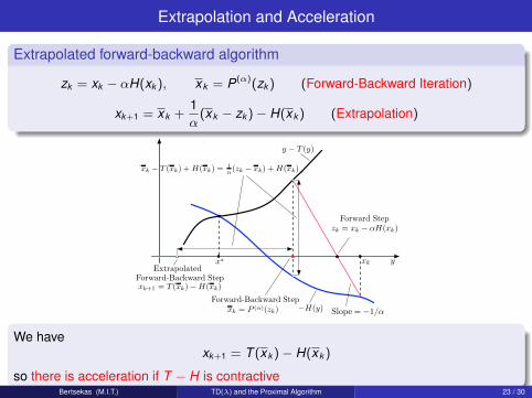
Extrapolation and Acceleration

Extrapolated forward-backward algorithm

zk = xk − αH(xk ), xk = P(α)(zk ) (Forward-Backward Iteration)

xk+1 = xk +1α

(xk − zk )− H(xk ) (Extrapolation)

λ Slope = −1/α

3 x∗

) y − T (y)

) Forward Step

) y −xk

zk = xk − αH(xk)

xk − T (xk) + H(xk) = 1α (zk − xk) + H(xk)

) Forward-Backward Step

) Forward-Backward Step

) xk = P (α)(zk)

Extrapolated Forward-Backward Step

Extrapolated Forward-Backward Step xk+1 = T (xk) − H(xk)

−H(y)

We havexk+1 = T (xk )− H(xk )

so there is acceleration if T − H is contractiveBertsekas (M.I.T.) TD(λ) and the Proximal Algorithm 23 / 30

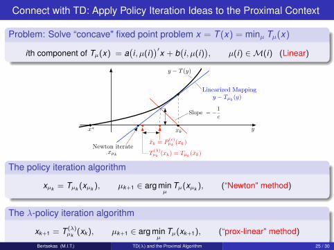
Connect with TD: Apply Policy Iteration Ideas to the Proximal Context

Problem: Solve “concave" fixed point problem x = T (x) = minµ Tµ(x)

i th component of Tµ(x) = a(i, µ(i)

)′x + b(i, µ(i)

), µ(i) ∈M(i) (Linear)

) y − T (y)

) y −

+2 Slope = −1

c

xk

Linearized Mapping

Newton iteratexµk

y − Tµk(y)

) xk = P(c)µk (xk)

) T(λ)µk (xk) = Tµk

(xk)

} x∗

The policy iteration algorithm

xµk = Tµk (xµk ), µk+1 ∈ arg minµ

Tµ(xµk ), (“Newton" method)

The λ-policy iteration algorithm

xk+1 = T (λ)µk (xk ), µk+1 ∈ arg min

µTµ(xk+1), (“prox-linear" method)


A Fundamental Difficulty

The algorithm chases a moving target

The TD(λ) mapping T (λ)µk “targets" the fixed point of Tµk , but as µk changes so

does the target ...

This is why some policy iteration algorithms may not converge (particularly withcost function approximation) ...


Convergence Under Monotonicity Assumptions

Assume the following:For all µ, the matrix Aµ has nonnegative components

The mappings Tµ are all contractions with respect to a common sup-norm (thiscan be relaxed ...)

Then:T is a contraction and its fixed point is x∗ = minµ xµA sequence {xk} generated from an initial condition x0 such that x0 ≥ T (x0) ismonotonically nonincreasing and converges to x∗ (this can be improved ...)

Proof idea:Based on DP/policy iteration arguments

Monotonicity is critical

Once projection is introduced in policy iteration, monotonicity may be lost


Convergence of Randomized Version Without Monotonicity

Assume the following:The setM is finite

The mappings Tµ and T are all contractions with respect to a common norm

We use a randomized form of the linearized iteration:

xk+1 = Tµk (xk ), with probability p,

xk+1 = T (λ)µk (xk ), with probability 1− p,

followed by µk+1 ∈ arg minµ Tµ(xk )

Then:For any starting point x0, a sequence {xk} generated by the algorithm converges to thefixed point of T with probability one

Randomization resolves the “moving target" problem


Concluding Remarks

Proximal and multistep/TD iterations for fixed point problems are closelyconnected

x , P(c)(x), and T (λ)(x) are colinear and simply related (no line search needed)

TD(λ) mapping is “faster" than proximal

A free lunch: Acceleration of the proximal algorithm. It can be substantial,particularly for small c

Extrapolation formula provides new insight and justification for TD-type methodsI TD(λ) is stochastic version of the proximal algorithmI TD(λ) with subspace approximation is stochastic version of the projected proximal

The ideas extend to the forward-backward algorithm and potentially otheralgorithmic contexts that involve fixed points and proximal operators

The relation between proximal and TD methods extends to classes of nonlinearfixed point problems using linearization/policy iteration ideas


Thank you!


TD() and the Proximal Algorithmdimitrib/Proximal_TD_Slides_NIPS.pdf · TD( ) and the Proximal...

Documents

Transcript of TD() and the Proximal Algorithmdimitrib/Proximal_TD_Slides_NIPS.pdf · TD( ) and the Proximal...