1

TCOM 501: Networking Theory & Fundamentals

Lectures 7

February 20, 2002

Prof. Yannis A. Korilis

7-2 Topics

Reversibility of Markov Chains Truncating a Reversible Markov Chain Time-Reversed Chain Burke’s Theorem Queues in Tandem

7-3 Time-Reversed Markov Chains

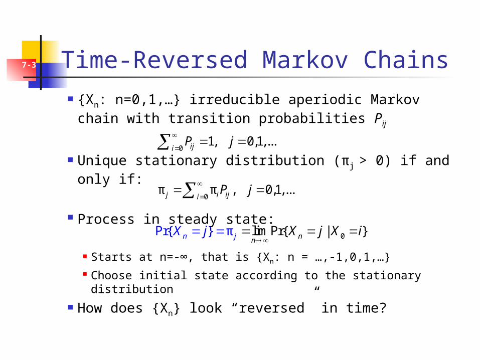
{Xn: n=0,1,…} irreducible aperiodic Markov chain with transition probabilities Pij

Unique stationary distribution (πj > 0) if and only if:

Process in steady state:

Starts at n=-∞, that is {Xn: n = …,-1,0,1,…} Choose initial state according to the stationary distribution

How does {Xn} look “reversed” in time?

0π π , 0,1,...j i iji

P j

01, 0,1,...iji

P j

0Pr{ } lim Pr |π { }nn

n j X XX ij j

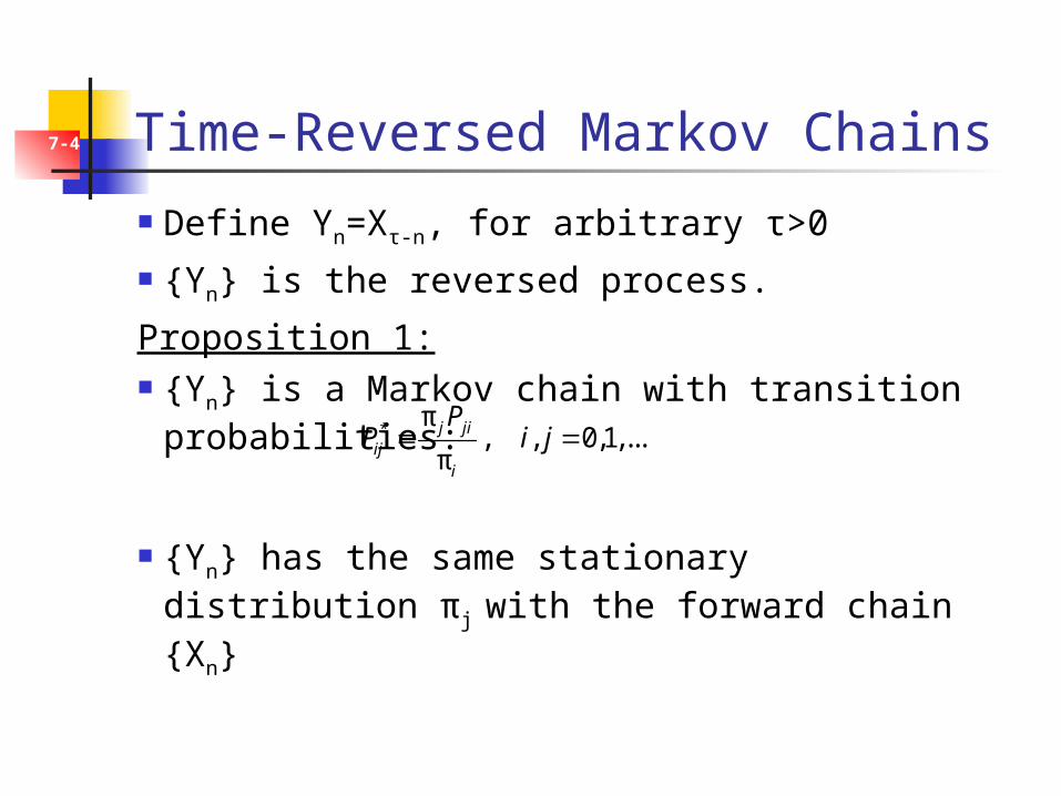
7-4 Time-Reversed Markov Chains

Define Yn=Xτ-n, for arbitrary τ>0

{Yn} is the reversed process.

Proposition 1: {Yn} is a Markov chain with transition probabilities:

{Yn} has the same stationary distribution πj with the forward chain {Xn}

* π, , 0,1,...

πj ji

iji

PP i j

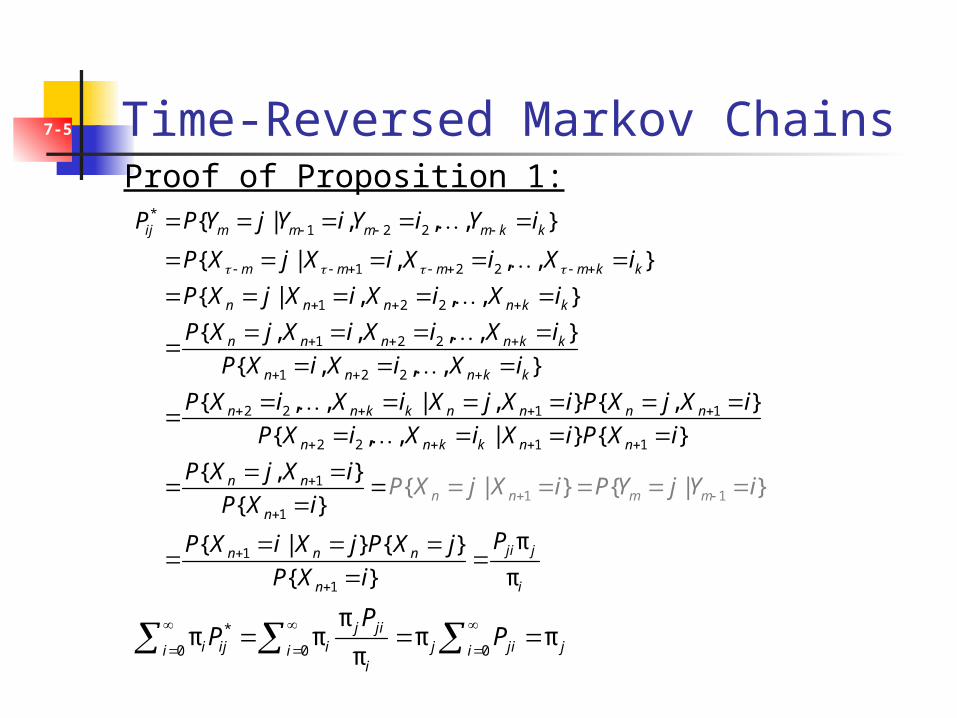
7-5 Time-Reversed Markov Chains

*1 2 2

1 2 2

1 2 2

1 2 2

1 2 2

2 2

{ | , , , }

{ | , , , }

{ | , , , }

{ , , , , }

{ , , , }

{ , , | ,

ij m m m m k k

m m m m k k

n n n n k k

n n n n k k

n n n k k

n n k k n n

P P Y j Y i Y i Y i

P X j X i X i X i

P X j X i X i X i

P X j X i X i X i

P X i X i X i

P X i X i X j X

1 1

2 2 1 1

1

1

1

1

1 1

} { , }

{ , , | } { }

{ , }

{ }

π{ | } { }

{ | } | }

{ } π

{

n n

n n k k n n

n nn n m

n

ji jn

m

n n

n i

i P X j X i

P X i X

P X j X i P Y

i X i P X i

P X j X i

P X i

PP X i X j P

j

X

Y i

j

P X i

*

0 0 0

ππ π π π

πj ji

i ij i j ji ji i ii

PP P

Proof of Proposition 1:

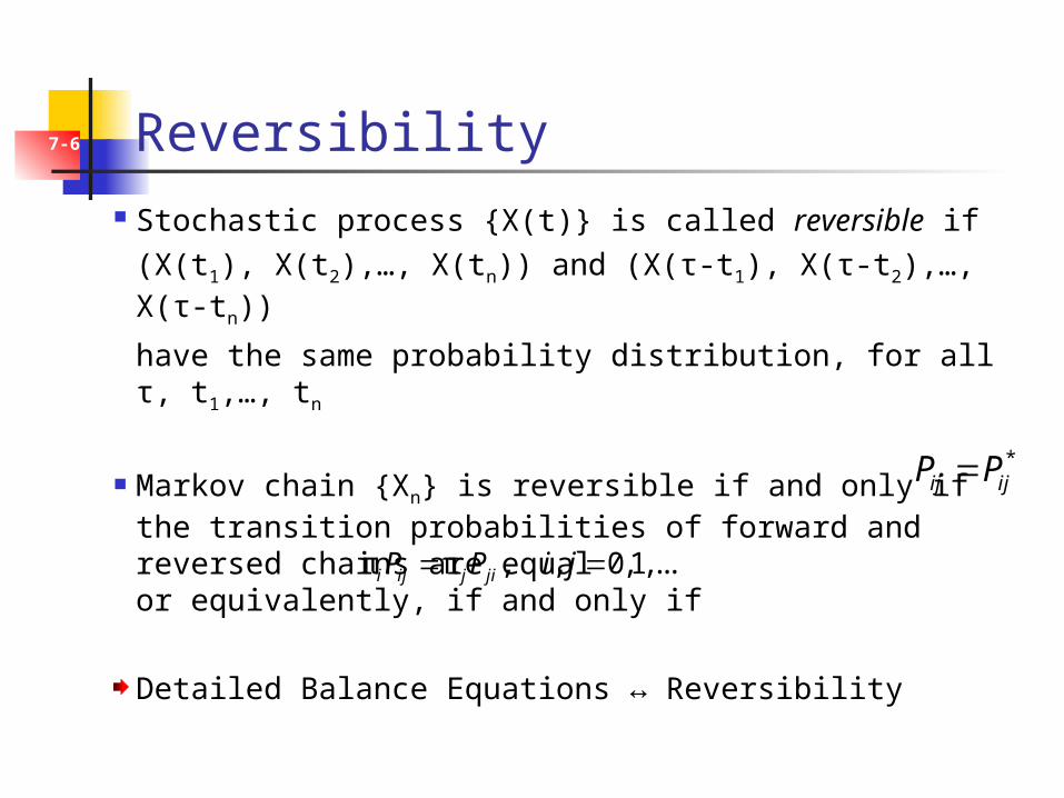
7-6 Reversibility

Stochastic process {X(t)} is called reversible if (X(t1), X(t2),…, X(tn)) and (X(τ-t1), X(τ-t2),…, X(τ-tn))

have the same probability distribution, for all τ, t1,…, tn

Markov chain {Xn} is reversible if and only if the transition probabilities of forward and reversed chains are equalor equivalently, if and only if

Detailed Balance Equations ↔ Reversibility

*ij ijP P

π π , , 0,1,...i ij j jiP P i j

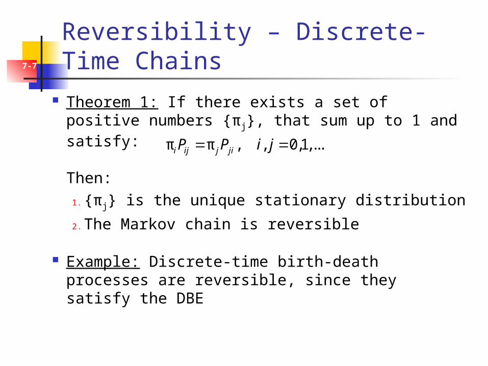
7-7 Reversibility – Discrete-Time Chains

Theorem 1: If there exists a set of positive numbers {πj}, that sum up to 1 and satisfy:

Then:

1. {πj} is the unique stationary distribution

2. The Markov chain is reversible

Example: Discrete-time birth-death processes are reversible, since they satisfy the DBE

π π , , 0,1,...i ij j jiP P i j

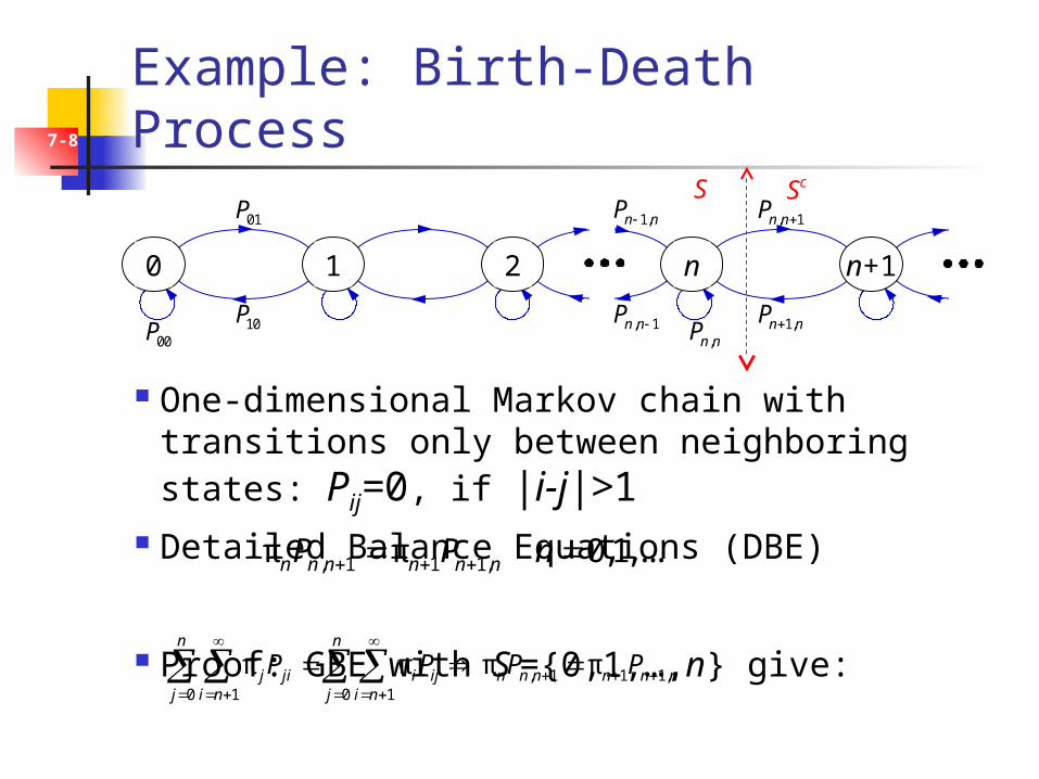
7-8 Example: Birth-Death Process

One-dimensional Markov chain with transitions only between neighboring states: Pij=0, if |i-j|>1

Detailed Balance Equations (DBE)

Proof: GBE with S ={0,1,…,n} give:

0 1 n+1n2

, 1n nP

1,n nP ,n nP, 1n nP

1,n nP 01P

10P00P

S Sc

, 1 1 1,π π 0,1,...n n n n n nP P n

, 1 1 1,0 1 0 1

π π π πn n

j ji i ij n n n n n nj i n j i n

P P P P

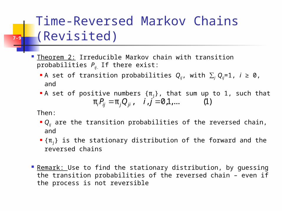
7-9 Time-Reversed Markov Chains (Revisited)

Theorem 2: Irreducible Markov chain with transition probabilities Pij. If there exist:

A set of transition probabilities Qij, with ∑j Qij=1, i ≥ 0, and

A set of positive numbers {πj}, that sum up to 1, such that

Then: Qij are the transition probabilities of the reversed chain, and

{πj} is the stationary distribution of the forward and the reversed chains

Remark: Use to find the stationary distribution, by guessing the transition probabilities of the reversed chain – even if the process is not reversible

π π , , 0,1,... (1)i ij j jiP Q i j

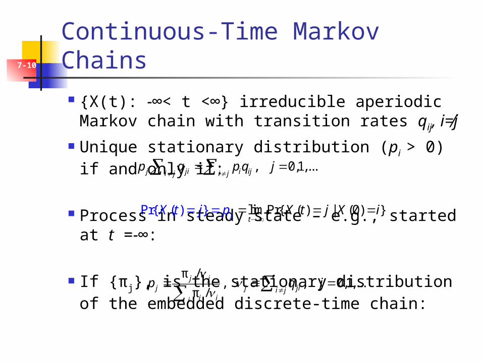
7-10 Continuous-Time Markov Chains

{X(t): -∞< t <∞} irreducible aperiodic Markov chain with transition rates qij, i≠j

Unique stationary distribution (pi > 0) if and only if:

Process in steady state – e.g., started at t =-∞:

If {πj}, is the stationary distribution of the embedded discrete-time chain:

, 0,1,...j ji i iji j i jp q p q j

limPr{ ( ) Pr{ ( ) | (0)} }t

j XX t t Xp j ij

π /, , 0,1,...

π /j j

j j jii ji ii

p q j

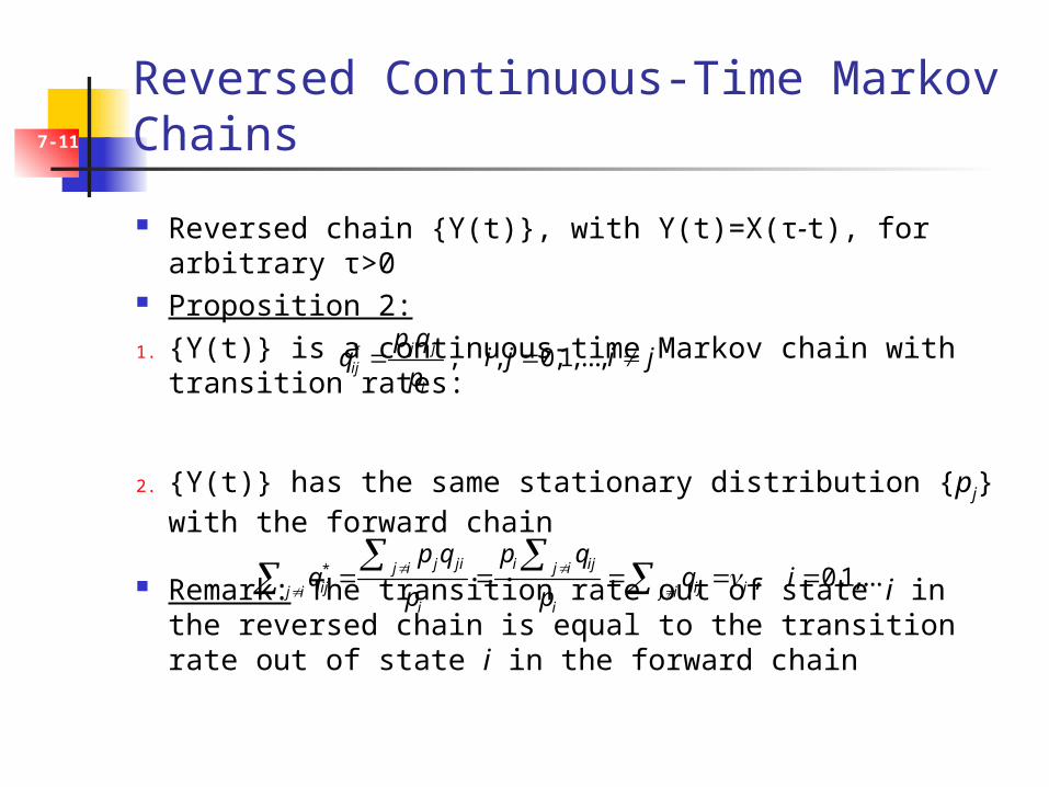
7-11 Reversed Continuous-Time Markov Chains

Reversed chain {Y(t)}, with Y(t)=X(τ-t), for arbitrary τ>0 Proposition 2:

1. {Y(t)} is a continuous-time Markov chain with transition rates:

2. {Y(t)} has the same stationary distribution {pj} with the forward chain

Remark: The transition rate out of state i in the reversed chain is equal to the transition rate out of state i in the forward chain

* , , 0,1,...,j jiij

i

p qq i j i j

p

* , 0,1,...j ji i ijj i j i

ij ij ij i j ii i

p q p qq q i

p p

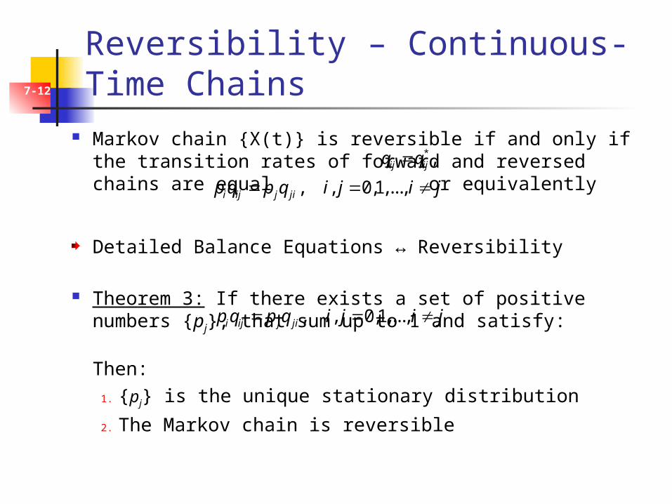
7-12 Reversibility – Continuous-Time Chains Markov chain {X(t)} is reversible if and only if the transition rates of

forward and reversed chains are equal or equivalently

Detailed Balance Equations ↔ Reversibility

Theorem 3: If there exists a set of positive numbers {pj}, that sum up to 1 and satisfy:

Then:

1. {pj} is the unique stationary distribution

2. The Markov chain is reversible

* ,ij ijq q

, , 0,1,...,i ij j jip q p q i j i j

, , 0,1,...,i ij j jip q p q i j i j

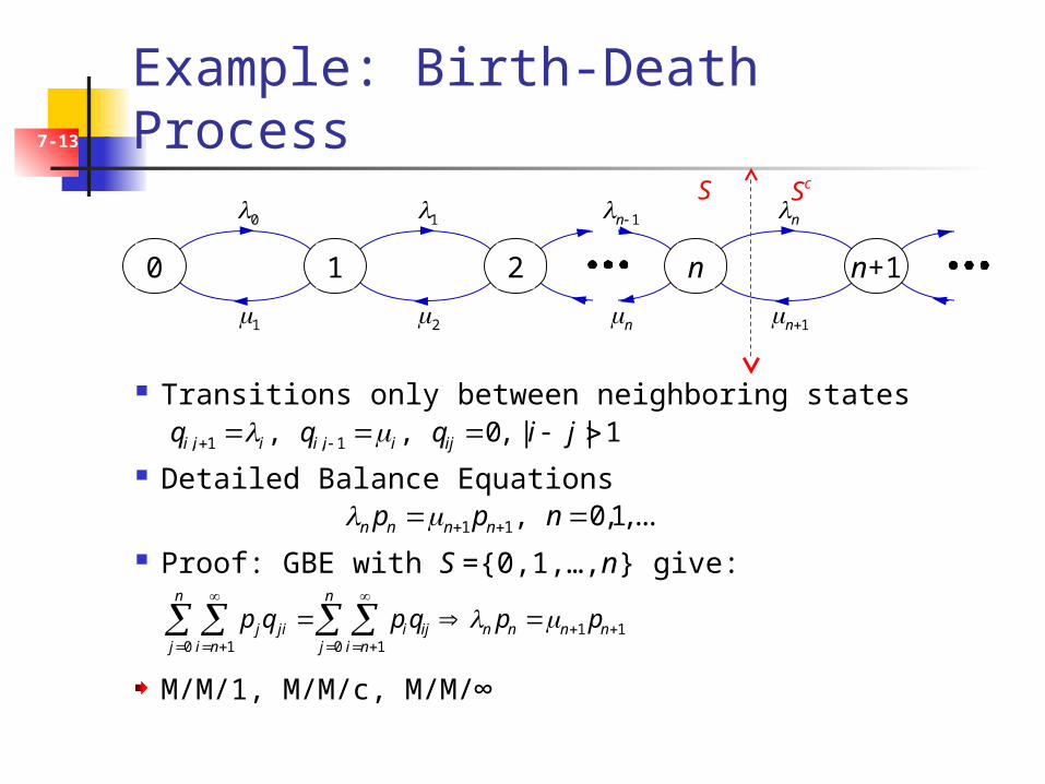
7-13 Example: Birth-Death Process

Transitions only between neighboring states

Detailed Balance Equations

Proof: GBE with S ={0,1,…,n} give:

M/M/1, M/M/c, M/M/∞

0 1 n+1n2

0

1

n

1n

1

2

1n

n

, 1 , 1, , 0, | | 1i i i i i i ijq q q i j

1 1, 0,1,...n n n np p n

1 10 1 0 1

n n

j ji i ij n n n nj i n j i n

p q p q p p

S Sc

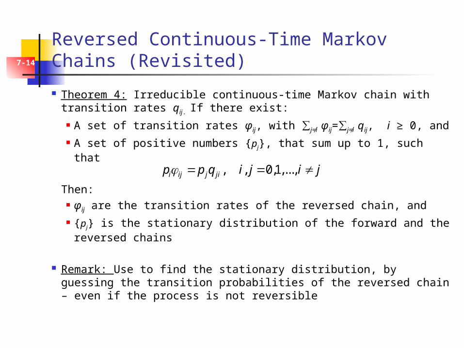
7-14 Reversed Continuous-Time Markov Chains (Revisited)

Theorem 4: Irreducible continuous-time Markov chain with transition rates qij. If there exist:

A set of transition rates φij, with ∑j≠i φij=∑j≠i qij, i ≥ 0, and

A set of positive numbers {pj}, that sum up to 1, such that

Then: φij are the transition rates of the reversed chain, and

{pj} is the stationary distribution of the forward and the reversed chains

Remark: Use to find the stationary distribution, by guessing the transition probabilities of the reversed chain – even if the process is not reversible

, , 0,1,...,i ij j jip p q i j i j

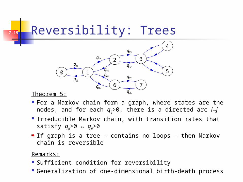
7-15 Reversibility: Trees

Theorem 5: For a Markov chain form a graph, where states are the nodes, and for

each qij>0, there is a directed arc i→j

Irreducible Markov chain, with transition rates that satisfy qij>0 ↔ qji>0

If graph is a tree – contains no loops – then Markov chain is reversible

Remarks: Sufficient condition for reversibility Generalization of one-dimensional birth-death process

01q

0 1

2

6

3

7

4

5

10q

12q

21q

16q

61q

23q

32q

67q

76q

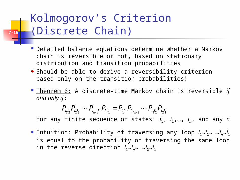
7-16 Kolmogorov’s Criterion (Discrete Chain)

Detailed balance equations determine whether a Markov chain is reversible or not, based on stationary distribution and transition probabilities

Should be able to derive a reversibility criterion based only on the transition probabilities!

Theorem 6: A discrete-time Markov chain is reversible if and only if:

for any finite sequence of states: i1, i2,…, in, and any n

Intuition: Probability of traversing any loop i1→i2→…→in→i1 is equal to the probability of traversing the same loop in the reverse direction i1→in→…→i2→i1

1 2 2 3 1 1 1 1 3 2 2 1n n n n n ni i i i i i i i i i i i i i i iP P P P P P P P

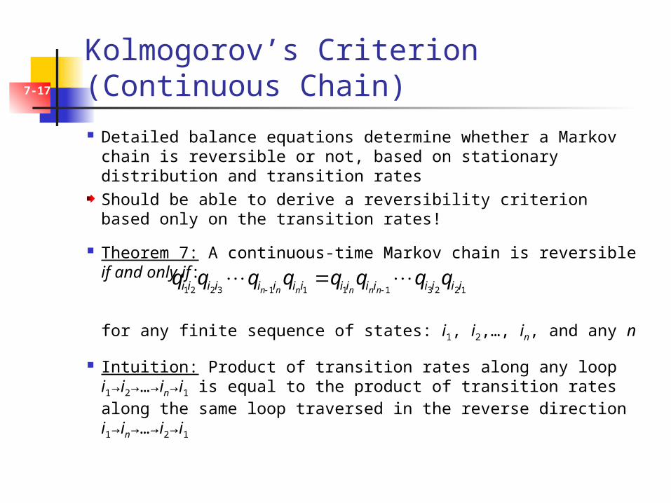
7-17 Kolmogorov’s Criterion (Continuous Chain)

Detailed balance equations determine whether a Markov chain is reversible or not, based on stationary distribution and transition rates

Should be able to derive a reversibility criterion based only on the transition rates!

Theorem 7: A continuous-time Markov chain is reversible if and only if:

for any finite sequence of states: i1, i2,…, in, and any n

Intuition: Product of transition rates along any loop i1→i2→…→in→i1 is equal to the product of transition rates along the same loop traversed in the reverse direction i1→in→…→i2→i1

1 2 2 3 1 1 1 1 3 2 2 1n n n n n ni i i i i i i i i i i i i i i iq q q q q q q q

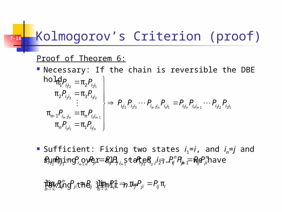
7-18 Kolmogorov’s Criterion (proof)

Proof of Theorem 6: Necessary: If the chain is reversible the DBE hold

Sufficient: Fixing two states i1=i, and in=j and summing over all states i2,…, in-1 we have

Taking the limit n→∞

1 2 2 1

2 3 3 2

1 2 2 3 1 1 1 1 3 2 2 1

1 1

1 1

1 2

2 3

1

1

π π

π π

π π

π π

n n n n n n

n n n n

n n

i i i i

i i i i

i i i i i i i i i i i i i i i i

n i i n i i

n i i i i

P P

P PP P P P P P P P

P P

P P

2 2 3 1 1 3 2 2, , , ,n n

n ni i i i i j ji ij j i i i i i ij ji ij jiP P P P P P P P P P P P

lim lim π πn nij ji ij ji j ji ij i

n nP P P P P P

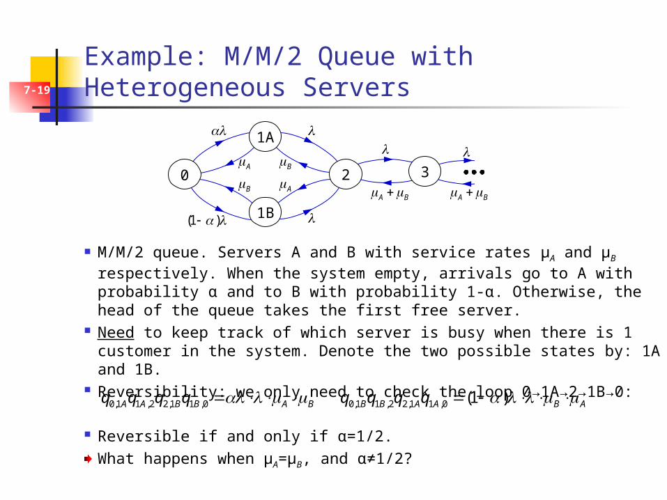
7-19 Example: M/M/2 Queue with Heterogeneous Servers

M/M/2 queue. Servers A and B with service rates μA and μB respectively. When the system empty, arrivals go to A with probability α and to B with probability 1-α. Otherwise, the head of the queue takes the first free server.

Need to keep track of which server is busy when there is 1 customer in the system. Denote the two possible states by: 1A and 1B.

Reversibility: we only need to check the loop 0→1A→2→1B→0:

Reversible if and only if α=1/2.

What happens when μA=μB, and α≠1/2?

0

1A

1B(1 )

A

B 2 3

B

AA B A B

0,1 1 ,2 2,1 1 ,0 0,1 1 ,2 2,1 1 ,0 (1 )A A B B A B B B A A B Aq q q q q q q q

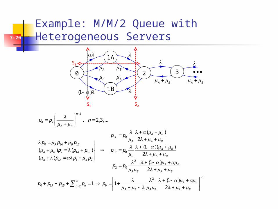
7-20 Example: M/M/2 Queue with Heterogeneous Servers

0

1A

1B(1 )

A

B 2 3

B

AA B A B

S1 S2

S3

2

2 , 2,3,...n

nA B

p p n

1 0

0 1 1

2 1 1 1 0

1 0 2 2

2 0

( )

2

(1 )( )( ) ( )

2( )

(1 )

2

A BA

A A BA A B B

A BA B A B B

B A BA A B

A B

A B A B

p p

p p p

p p p p p

p p p

p p

12

0 1 1 02

(1 )1 1

2A B

A B nnA B A B A B

p p p p p

7-21 Multidimensional Markov Chains

Theorem 8: {X1(t)}, {X2(t)}: independent Markov chains

{Xi(t)}: reversible

{X(t)}, with X(t)=(X1(t), X2(t)): vector-valued stochastic process

{X(t)} is a Markov chain

{X(t)} is reversible

Multidimensional Chains: Queueing system with two classes of customers, each having its own

stochastic properties – track the number of customers from each class Study the “joint” evolution of two queueing systems – track the number

of customers in each system

7-22 Example: Two Independent M/M/1 Queues

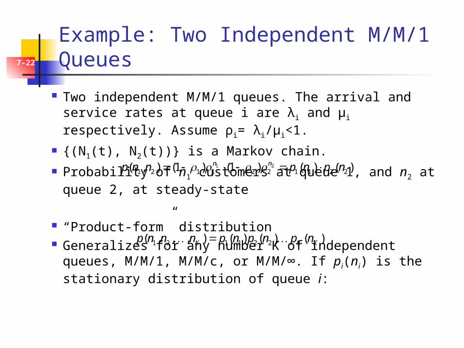
Two independent M/M/1 queues. The arrival and service rates at queue i are λi and μi respectively. Assume ρi= λi/μi<1.

{(N1(t), N2(t))} is a Markov chain.

Probability of n1 customers at queue 1, and n2 at queue 2, at steady-state

“Product-form” distribution Generalizes for any number K of independent queues, M/M/1, M/M/c,

or M/M/∞. If pi(ni) is the stationary distribution of queue i:

1 21 2 1 1 2 2 1 1 2 2( , ) (1 ) (1 ) ( ) ( )n np n n p n p n

1 2 1 1 2 2( , , , ) ( ) ( ) ( )K K Kp n n n p n p n p n

7-23

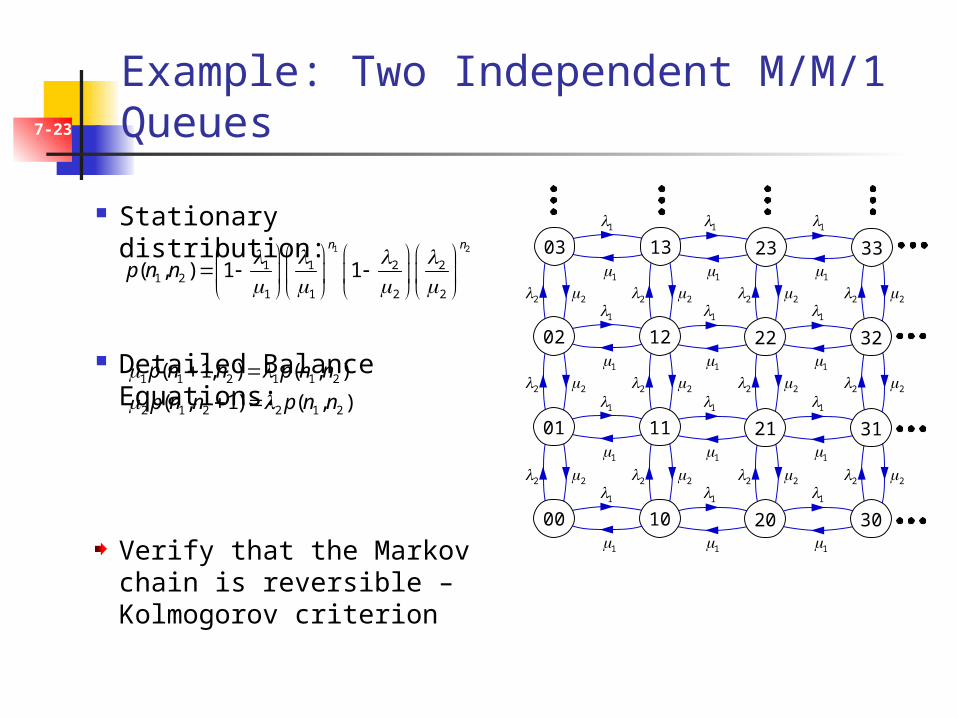
Stationary distribution:

Detailed Balance Equations:

Verify that the Markov chain is reversible – Kolmogorov criterion

Example: Two Independent M/M/1 Queues

1 2

1 1 2 21 2

1 1 2 2

( , ) 1 1n n

p n n

1 1 2 1 1 2

2 1 2 2 1 2

( 1, ) ( , )

( , 1) ( , )

p n n p n n

p n n p n n

2 22 2 2 2 2 2

2 22 2 2 2 2 2

2 22 2 2 2 2 2

02 12 22 321 1 1

1 1 1

01 11 21 311 1 1

1 1 1

00 10 20 301 1 1

1 1 1

03 13 23 331 1 1

1 1 1

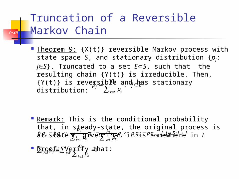
7-24 Truncation of a Reversible Markov Chain

Theorem 9: {X(t)} reversible Markov process with state space S, and stationary distribution {pj: jS}. Truncated to a set ES, such that the resulting chain {Y(t)} is irreducible. Then, {Y(t)} is reversible and has stationary distribution:

Remark: This is the conditional probability that, in steady-state, the original process is at state j, given that it is somewhere in E

Proof: Verify that:

,jj

kk E

pp j E

p

, , ;

1

j ij ji i ij ji ij j ji i ij

k kk E k E

jjj E j E

kk E

p pp q p q q q p q p q i j S i j

p p

pp

p

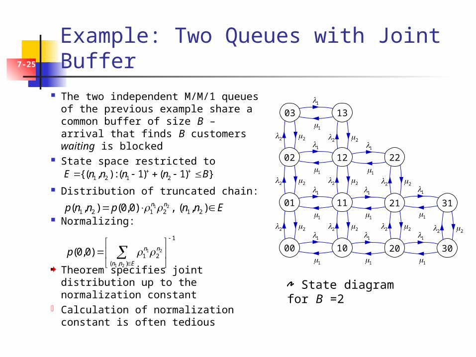
7-25 Example: Two Queues with Joint Buffer

The two independent M/M/1 queues of the previous example share a common buffer of size B – arrival that finds B customers waiting is blocked

State space restricted to

Distribution of truncated chain:

Normalizing:

Theorem specifies joint distribution up to the normalization constant

Calculation of normalization constant is often tedious

2 2

2 2

2 21

1

2 2

2 2

2 2

1

1

1

1

1

1

2 2

2 2 2 2

02 121

1

01 11 211 1

1 1

00 10 20 301 1

1 1

03 13

22

31

1 2 1 2{( , ) : ( 1) ( 1) }E n n n n B

1 21 2 1 2 1 2( , ) (0,0) , ( , )n np n n p n n E

1 2

1 2

1

1 2( , )

(0,0) n n

n n E

p

State diagram for B =2

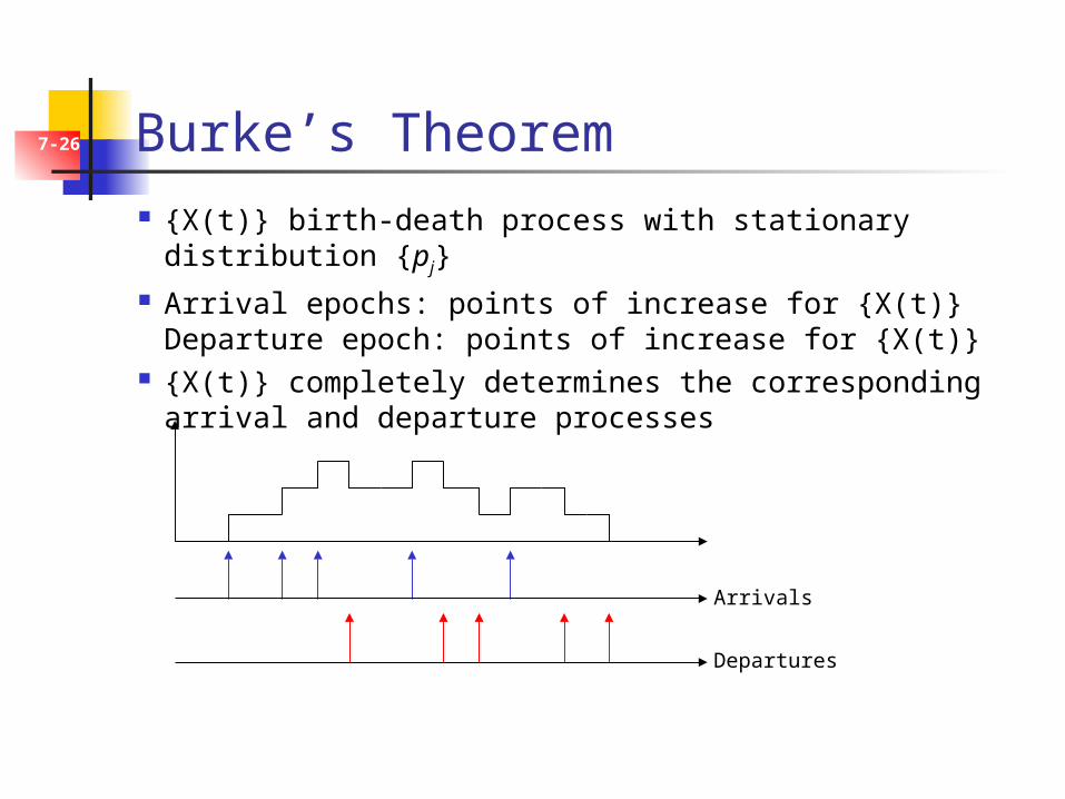
7-26 Burke’s Theorem

{X(t)} birth-death process with stationary distribution {pj} Arrival epochs: points of increase for {X(t)}

Departure epoch: points of increase for {X(t)} {X(t)} completely determines the corresponding arrival and departure

processes

Arrivals

Departures

7-27 Burke’s Theorem Poisson arrival process: λj=λ, for all j

Birth-death process called a (λ, μj)-process Examples: M/M/1, M/M/c, M/M/∞ queues

Poisson arrivals → LAA: For any time t, future arrivals are independent of {X(s): s≤t}

(λ, μj)-process at steady state is reversible: forward and reversed chains are stochastically identicalArrival processes of the forward and reversed chains are stochastically identical

Arrival process of the reversed chain is Poisson with rate λ The arrival epochs of the reversed chain are the departure epochs of the

forward chainDeparture process of the forward chain is Poisson with rate λ

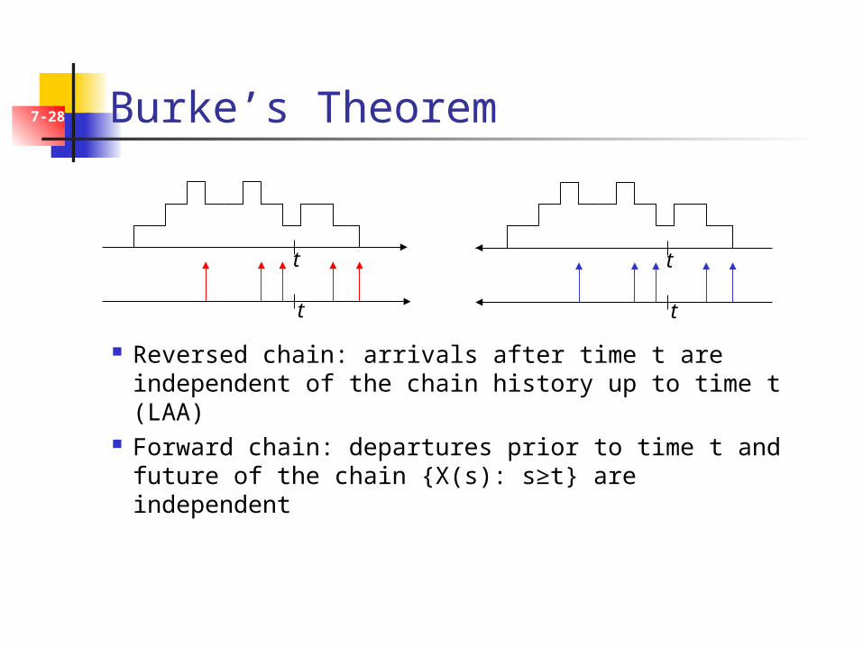
7-28 Burke’s Theorem

Reversed chain: arrivals after time t are independent of the chain history up to time t (LAA)

Forward chain: departures prior to time t and future of the chain {X(s): s≥t} are independent

t

t

t

t

7-29 Burke’s Theorem Theorem 10: Consider an M/M/1, M/M/c, or M/M/∞ system with

arrival rate λ. Suppose that the system starts at steady-state. Then:

1. The departure process is Poisson with rate λ

2. At each time t, the number of customers in the system is independent of the departure times prior to t

Fundamental result for study of networks of M/M/* queues, where output process from one queue is the input process of another

7-30 Single-Server Queues in Tandem

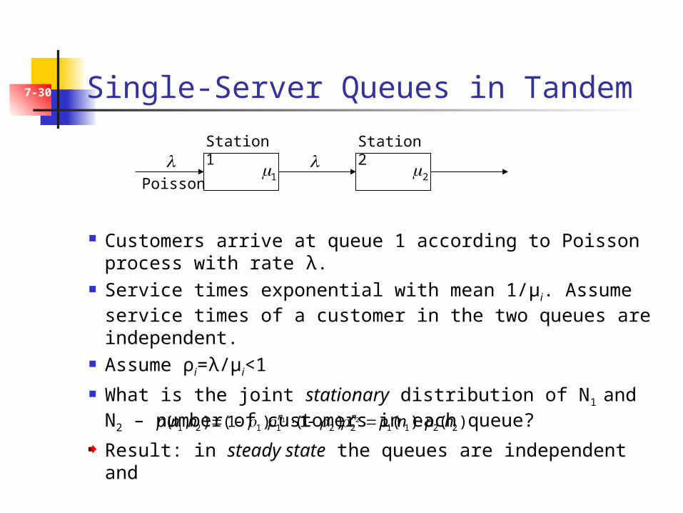
Customers arrive at queue 1 according to Poisson process with rate λ. Service times exponential with mean 1/μi. Assume service times of a

customer in the two queues are independent. Assume ρi=λ/μi<1

What is the joint stationary distribution of N1 and N2 – number of customers in each queue?

Result: in steady state the queues are independent and 1 2

1 2 1 1 2 2 1 1 2 2( , ) (1 ) (1 ) ( ) ( )n np n n p n p n

Poisson 1 2

Station 1 Station 2

7-31 Single-Server Queues in Tandem

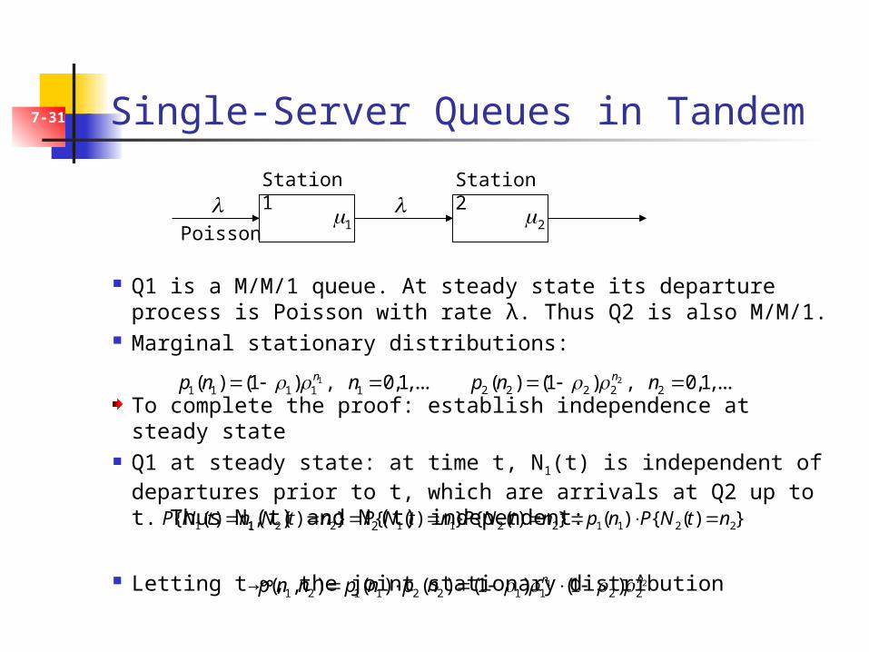
Q1 is a M/M/1 queue. At steady state its departure process is Poisson with rate λ. Thus Q2 is also M/M/1.

Marginal stationary distributions:

To complete the proof: establish independence at steady state Q1 at steady state: at time t, N1(t) is independent of departures prior to t,

which are arrivals at Q2 up to t. Thus N1(t) and N2(t) independent:

Letting t→∞, the joint stationary distribution1 2

1 2 1 1 2 2 1 1 2 2( , ) ( ) ( ) (1 ) (1 )n np n n p n p n

Poisson 1 2

Station 1 Station 2

11 1 1 1 1( ) (1 ) , 0,1,...np n n 2

2 2 2 2 2( ) (1 ) , 0,1,...np n n

1 1 2 2 1 1 2 2 1 1 2 2{ ( ) , ( ) } { ( ) } { ( ) } ( ) { ( ) }P N t n N t n P N t n P N t n p n P N t n

7-32 Queues in Tandem

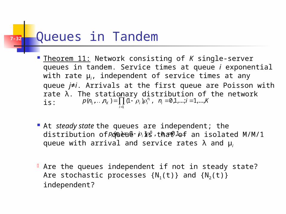
Theorem 11: Network consisting of K single-server queues in tandem. Service times at queue i exponential with rate μi, independent of service times at any queue j≠i. Arrivals at the first queue are Poisson with rate λ. The stationary distribution of the network is:

At steady state the queues are independent; the distribution of queue i is that of an isolated M/M/1 queue with arrival and service rates λ and μi

Are the queues independent if not in steady state? Are stochastic processes {N1(t)} and {N2(t)} independent?

11

( , , ) (1 ) , 0,1,...; 1,...,i

Kn

K i i ii

p n n n i K

( ) (1 ) , 0,1,...ini i i i ip n n

7-33 Queues in Tandem: State-Dependent Service Rates

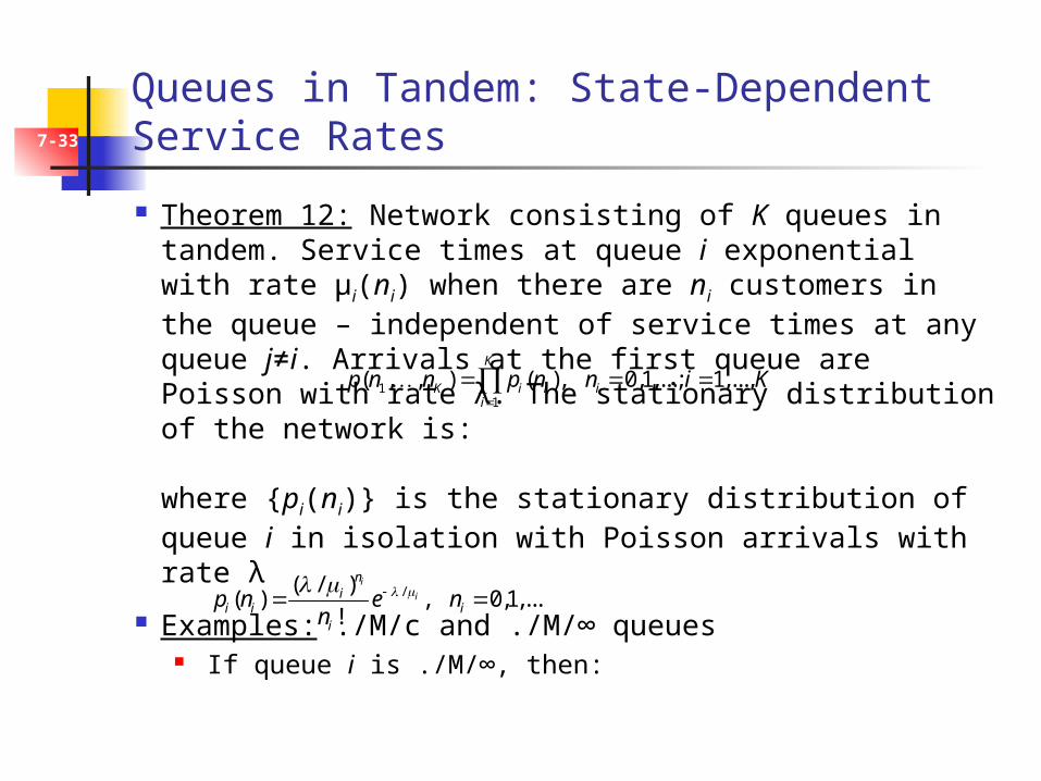
Theorem 12: Network consisting of K queues in tandem. Service times at queue i exponential with rate μi(ni) when there are ni customers in the queue – independent of service times at any queue j≠i. Arrivals at the first queue are Poisson with rate λ. The stationary distribution of the network is:

where {pi(ni)} is the stationary distribution of queue i in isolation with Poisson arrivals with rate λ

Examples: ./M/c and ./M/∞ queues If queue i is ./M/∞, then:

11

( , , ) ( ), 0,1,...; 1,...,K

K i i ii

p n n p n n i K

/( / )( ) , 0,1,...

!

i

i

ni

i i ii

p n e nn