T-UGOm :the Toulouse Unstructured

Grid Ocean model

F. Lyard 1, C. Nguyen 1, C. Mayet 1, Y. Soufflet 1

D. Greenberg 2, F. Dupont 3

1LEGOS, CNRS, Toulouse2BIO, Halifax, Nova Scottia

3Environement Canada, Montreal

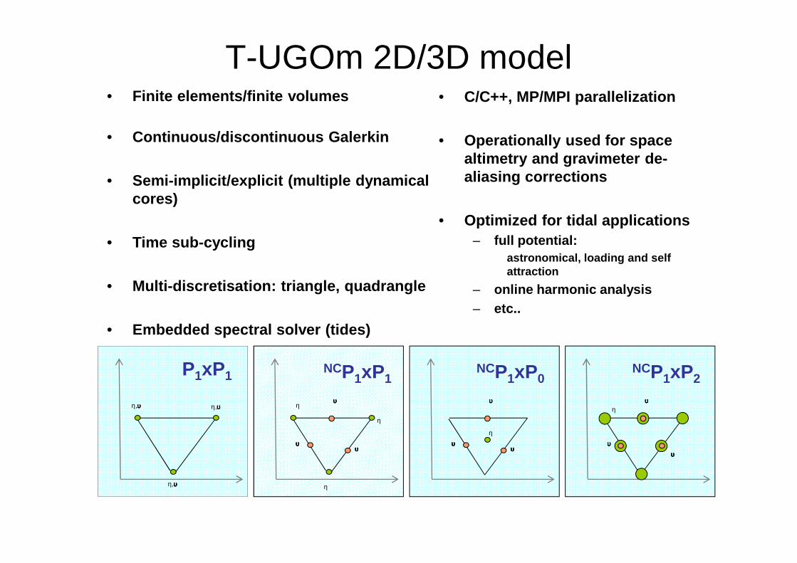
T-UGOm 2D/3D model

η,υυυυ

η,υυυυ

η,υυυυ

P1xP1

η

η

ηυυυυ

υυυυυυυυ

NCP1xP1

η

υυυυ

υυυυυυυυ

NCP1xP0

ηυυυυ

υυυυυυυυ

NCP1xP2

• Finite elements/finite volumes

• Continuous/discontinuous Galerkin

• Semi-implicit/explicit (multiple dynamical cores)

• Time sub-cycling

• Multi-discretisation: triangle, quadrangle

• Embedded spectral solver (tides)

• C/C++, MP/MPI parallelization

• Operationally used for space altimetry and gravimeter de-aliasing corrections

• Optimized for tidal applications– full potential:

astronomical, loading and self attraction

– online harmonic analysis– etc..

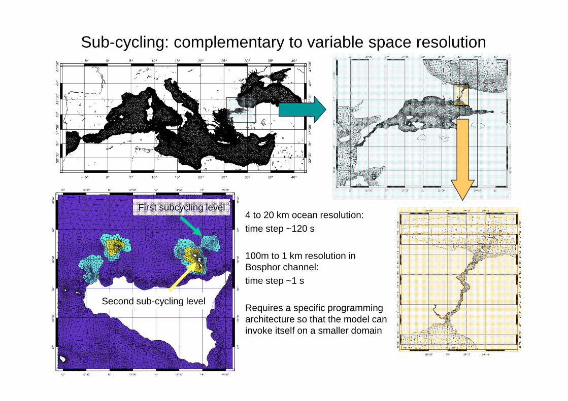
Sub-cycling: complementary to variable space resolution

• Automatic or constrained sub-cycling

First subcycling level

Second sub-cycling level

4 to 20 km ocean resolution:time step ~120 s

100m to 1 km resolution in Bosphor channel:time step ~1 s

Requires a specific programming architecture so that the model can invoke itself on a smaller domain

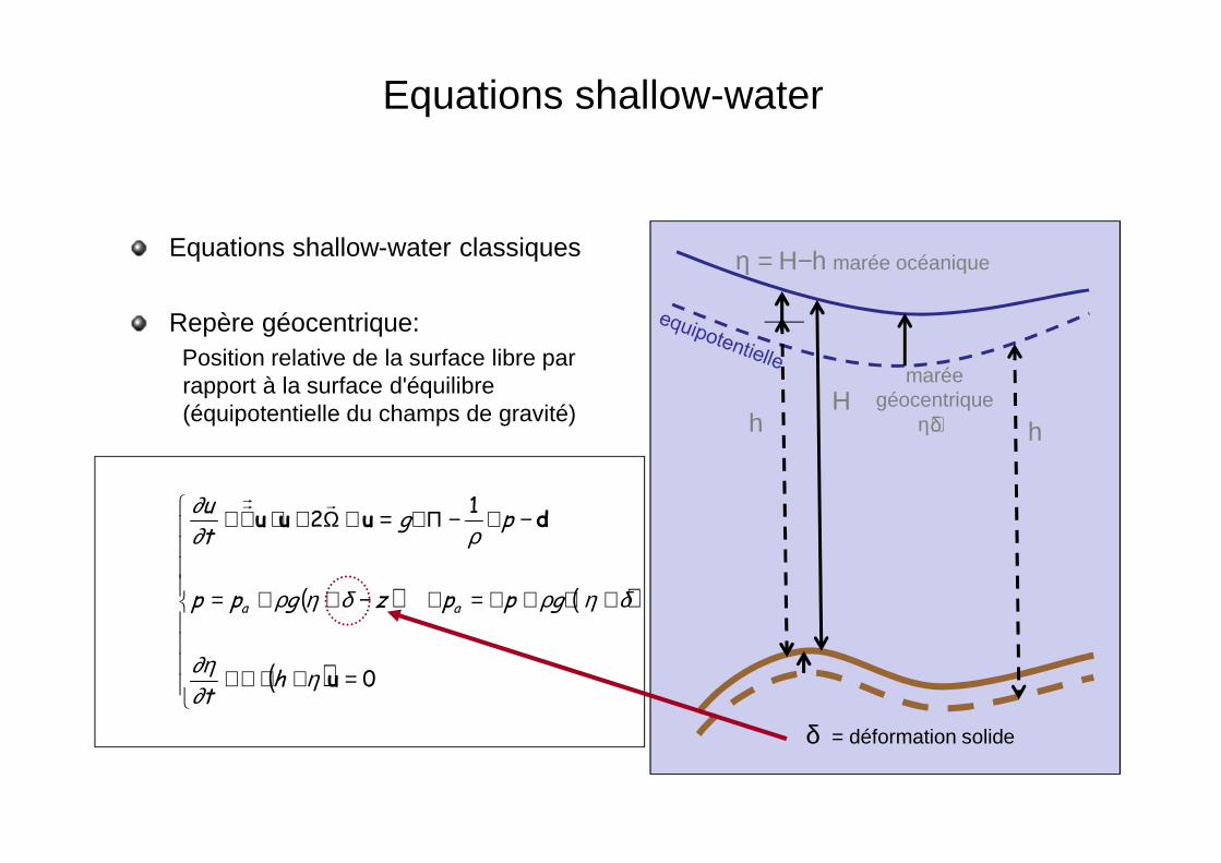
Equations shallow-water

( ) ( )

( )

=+⋅∇+

+∇+∇=∇−++=

−∇−Π∇=∧Ω+⋅∇+

0

12

u

duuu

η∂∂η

δηρδηρ

ρ∂∂

ht

gppzgpp

pgtu

aa

rrr

hH

δ = déformation solide

η = Η−h marée océaniqueEquations shallow-water classiques

Repère géocentrique:Position relative de la surface libre par rapport à la surface d'équilibre (équipotentielle du champs de gravité) h

maréegéocentrique

η+δ

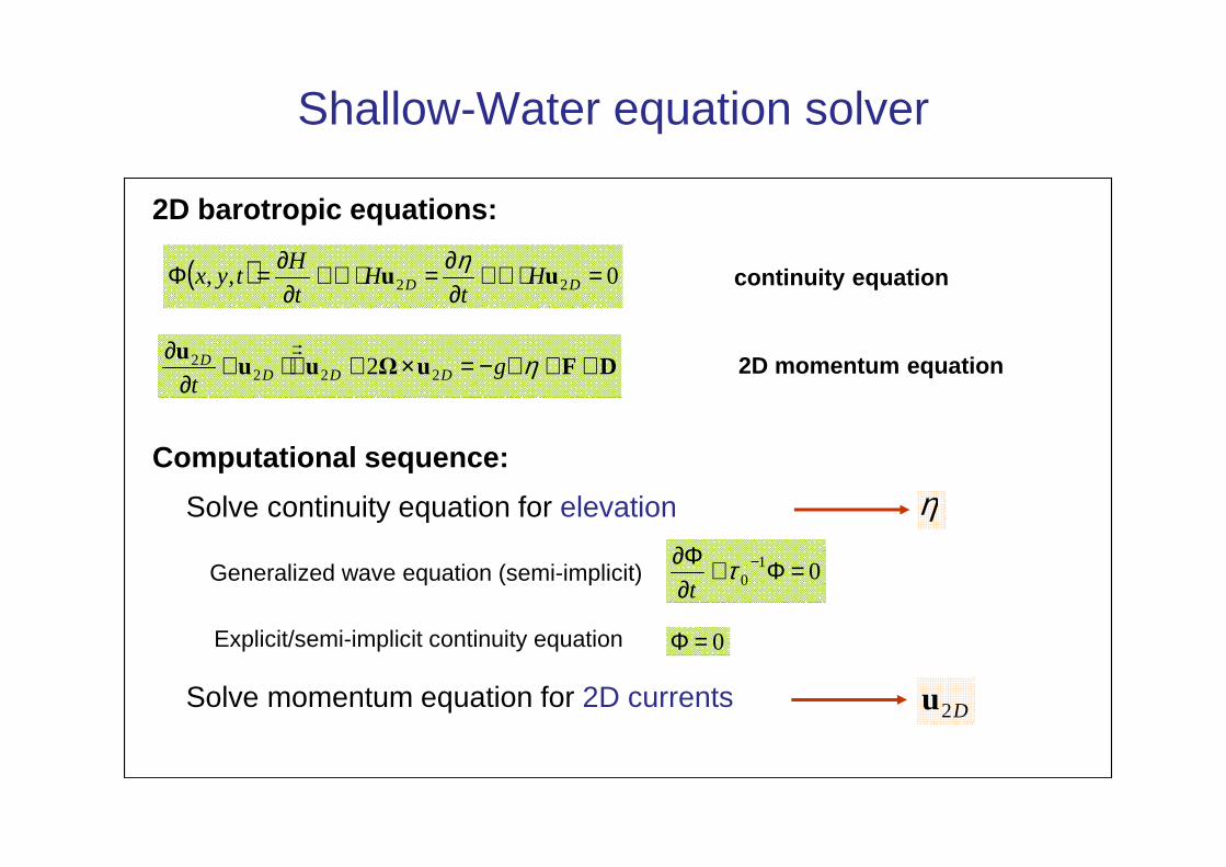
Shallow-Water equation solver

( ) 0,, 22 =⋅∇+∂∂=⋅∇+

∂∂=Φ DD H

tH

t

Htyx uu

η

DFuΩuuu ++∇−=×+∇⋅+∂

∂ ηgt DDD

D222

2 2rr

Computational sequence:

010 =Φ+

∂Φ∂ −τt

Solve continuity equation for elevation

Solve momentum equation for 2D currents

η

D2u

0=Φ

Generalized wave equation (semi-implicit)

Explicit/semi-implicit continuity equation

continuity equation

2D momentum equation

2D barotropic equations:

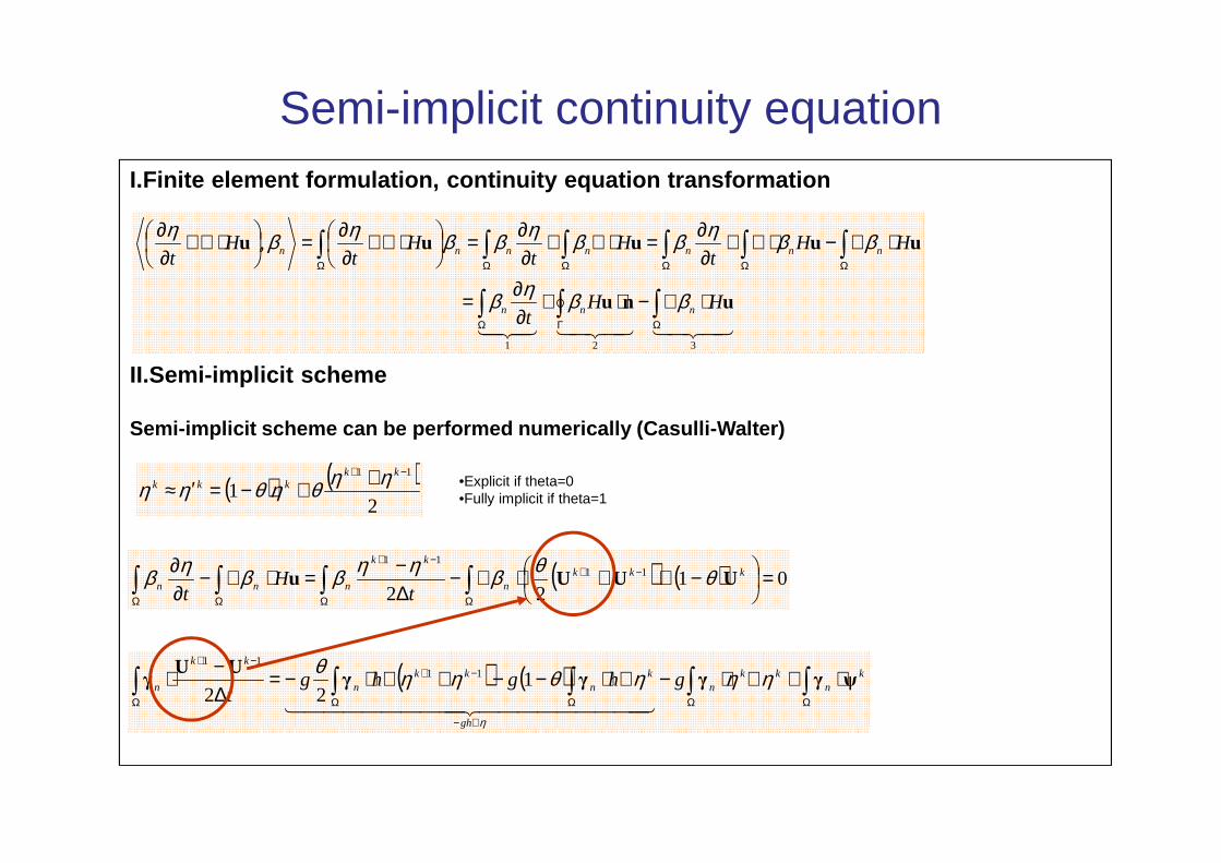
I.Finite element formulation, continuity equation t ransformation

II.Semi-implicit scheme

Semi-implicit scheme can be performed numerically ( Casulli-Walter)

Semi-implicit continuity equation

434214342143421321

,

∫∫∫

∫∫∫∫∫∫

ΩΓΩ

ΩΩΩΩΩΩ

⋅∇−⋅+∂∂=

⋅∇−⋅∇+∂∂=⋅∇+

∂∂=

⋅∇+∂∂=

⋅∇+∂∂

unu

uuuuu

HHt

HHt

Ht

Ht

Ht

nnn

nnnnnnn

ββηβ

ββηββηββηβη

( ) ( ) 0122

1111

=

−++⋅∇−∆−=⋅∇−

∂∂

∫∫∫∫Ω

−+

Ω

−+

ΩΩ

kkkn

kk

nnn tH

tUUUu θθβηηββηβ

( ) ( ) ∫∫∫∫∫ΩΩ

∇−

ΩΩ

−+

Ω

−+

⋅+∇⋅−∇⋅−−+∇⋅−=∆−⋅ k

nkk

n

gh

kn

kkn

kk

n ghghgt

ψγγγγUU

γ ηηηθηηθ

η444444444 3444444444 21

122

1111

( ) ( )2

111 −+ ++−=′≈

kkkkk ηηθηθηη •Explicit if theta=0

•Fully implicit if theta=1

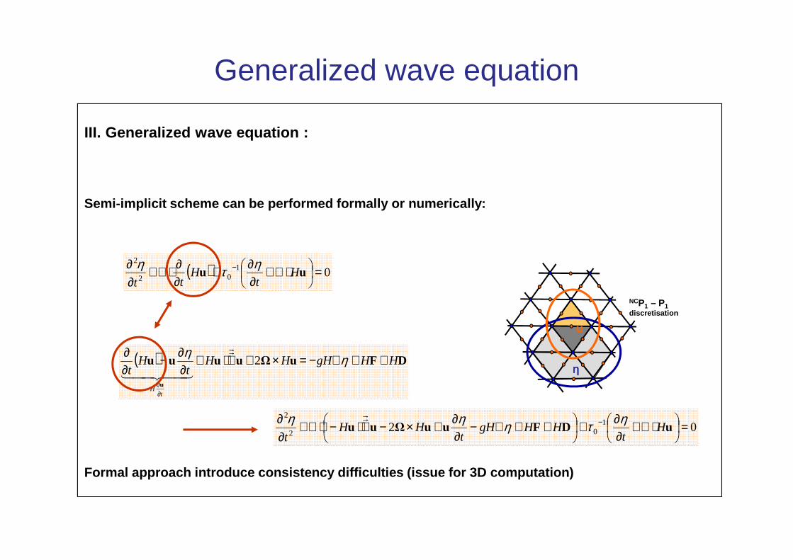
III. Generalized wave equation :

Semi-implicit scheme can be performed formally or n umerically:

Formal approach introduce consistency difficulties (issue for 3D computation)

( ) DFuΩuuuu

u

HHgHHHt

Ht

tH

++∇−=×+∇⋅+∂∂−

∂∂

∂∂

ηη2

rr

44 344 21

( ) 0102

2

=

⋅∇+∂∂+

∂∂⋅∇+

∂∂ − uu H

tH

tt

ητη

02 102

2

=

⋅∇+∂∂+

++∇−∂∂+×−∇⋅−⋅∇+

∂∂ − uDFuuΩuu H

tHHgH

tHH

t

ητηηη rr

Generalized wave equation

u

ηηηη

NCP1 – P1discretisation

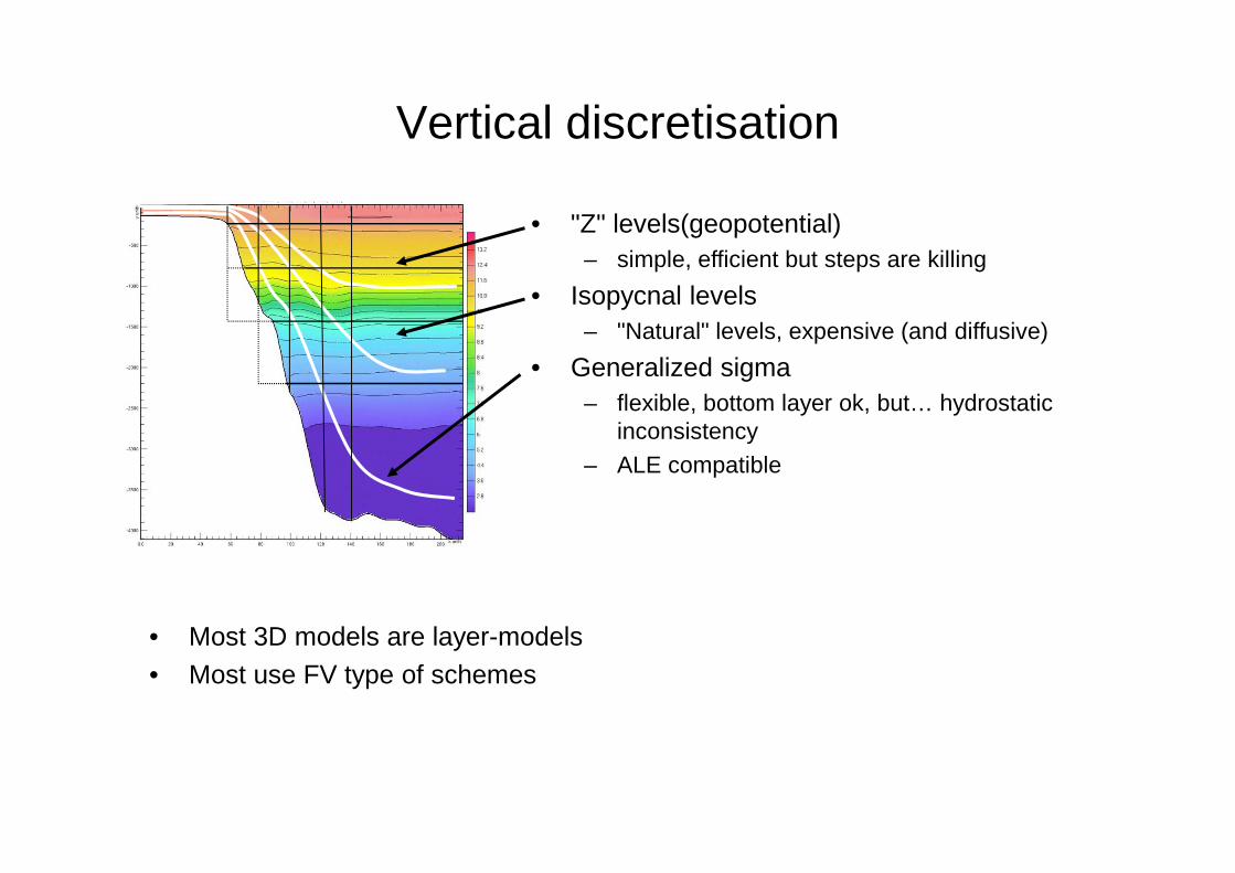
Vertical discretisation

• "Z" levels(geopotential)– simple, efficient but steps are killing

• Isopycnal levels– "Natural" levels, expensive (and diffusive)

• Generalized sigma– flexible, bottom layer ok, but… hydrostatic

inconsistency– ALE compatible

• Most 3D models are layer-models• Most use FV type of schemes

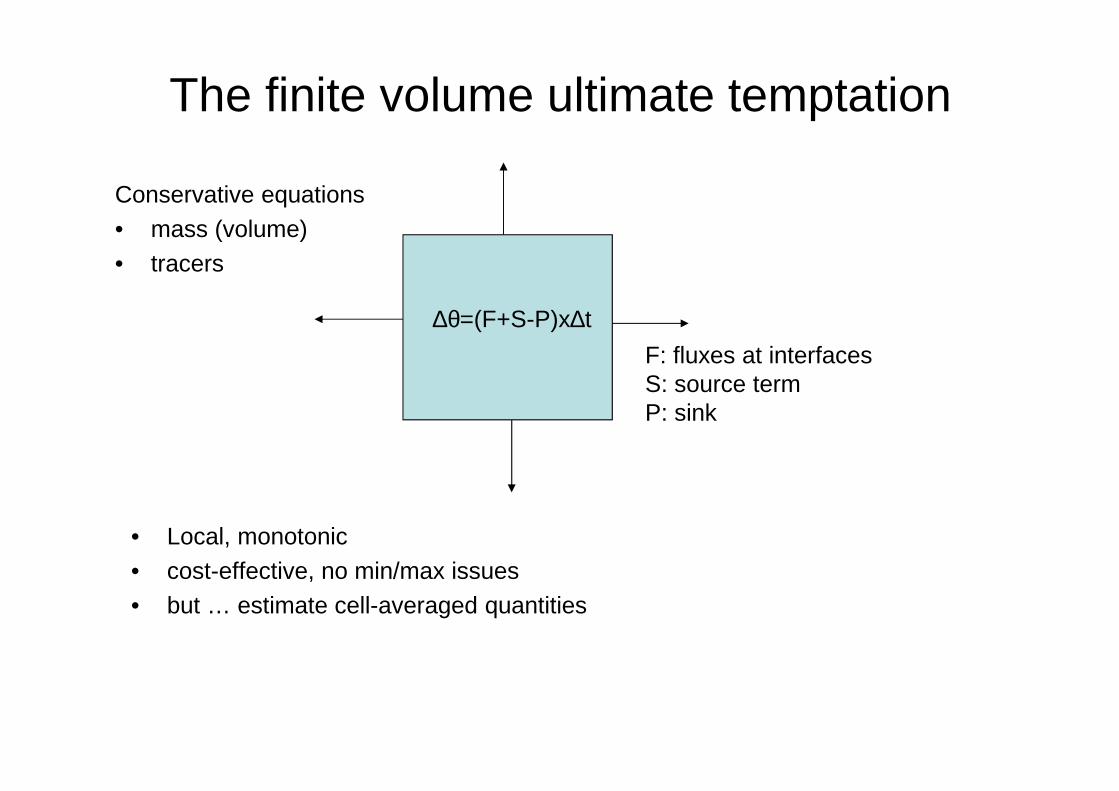
The finite volume ultimate temptation

• Local, monotonic• cost-effective, no min/max issues• but … estimate cell-averaged quantities

∆θ=(F+S-P)x∆t

Conservative equations• mass (volume)• tracers

F: fluxes at interfacesS: source termP: sink

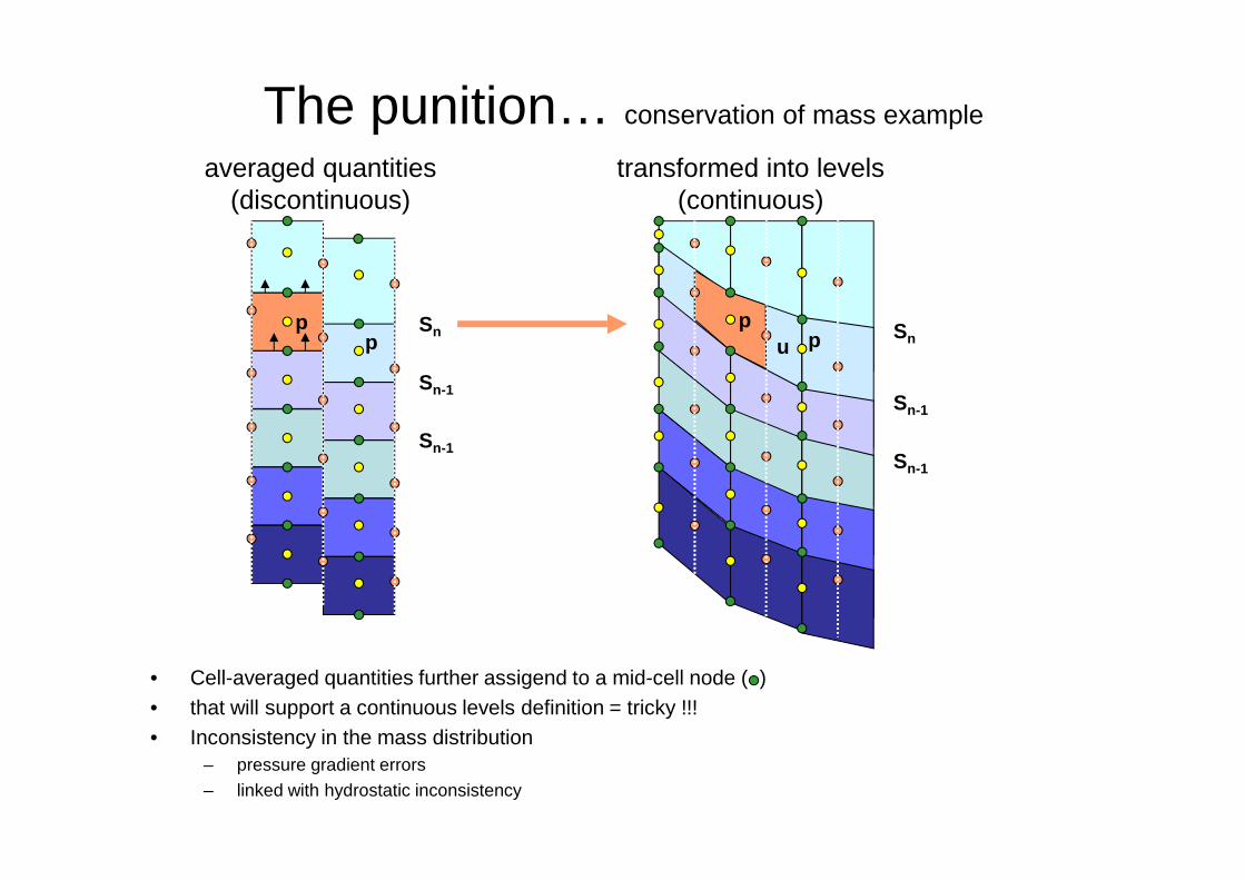
The punition… conservation of mass example

• Cell-averaged quantities further assigend to a mid-cell node ( )• that will support a continuous levels definition = tricky !!!• Inconsistency in the mass distribution

– pressure gradient errors– linked with hydrostatic inconsistency

up

Sn-1

Sn-1

averaged quantities(discontinuous)

p Snp

Sn-1

Sn-1

pSn

transformed into levels(continuous)

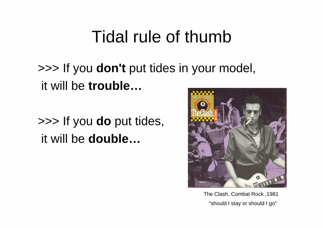
Tidal rule of thumb

>>> If you don't put tides in your model,it will be trouble…

>>> If you do put tides, it will be double…

The Clash, Combat Rock ,1981

"should I stay or should I go"

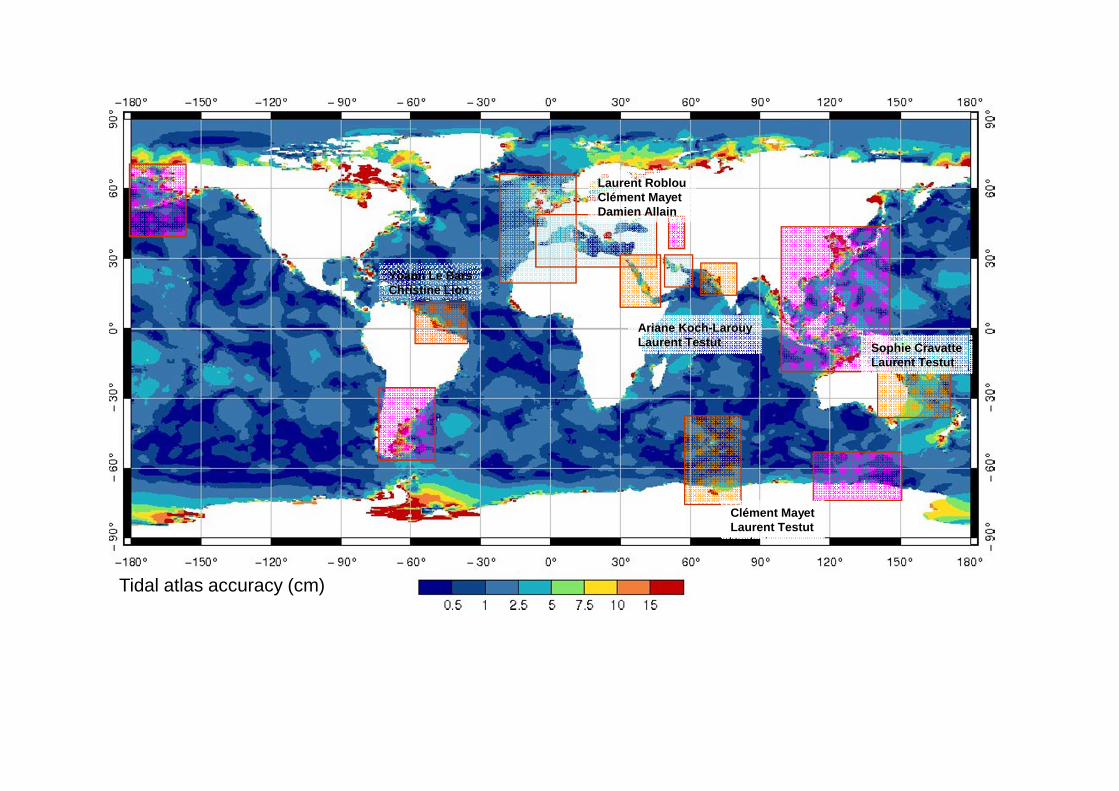
Tidal atlas accuracy (cm)

Ariane Koch-LarouyLaurent Testut

Yoann Le BarsChristine Lion

Sophie CravatteLaurent Testut

Laurent RoblouClément MayetDamien Allain

Clément MayetLaurent Testut

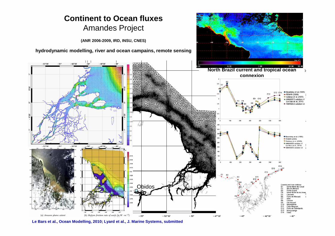
Obidos

North Brazil current and tropical ocean connexion

Continent to Ocean fluxesAmandes Project

(ANR 2006-2009, IRD, INSU, CNES)

hydrodynamic modelling, river and ocean campains, r emote sensing

Le Bars et al., Ocean Modelling, 2010; Lyard et al. , J. Marine Systems, submitted

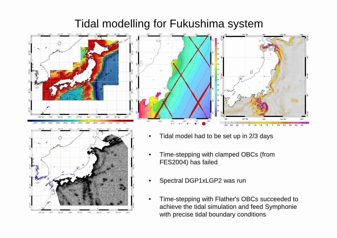
Tidal modelling for Fukushima system

• Tidal model had to be set up in 2/3 days

• Time-stepping with clamped OBCs (from FES2004) has failed

• Spectral DGP1xLGP2 was run

• Time-stepping with Flather's OBCs succeeded to achieve the tidal simulation and feed Symphonie with precise tidal boundary conditions

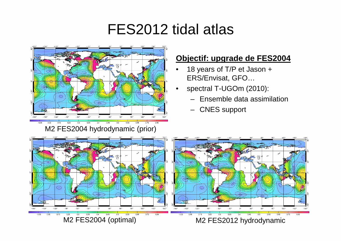
FES2012 tidal atlas

Objectif: upgrade de FES2004• 18 years of T/P et Jason +

ERS/Envisat, GFO… • spectral T-UGOm (2010):

– Ensemble data assimilation– CNES support

M2 FES2004 hydrodynamic (prior)

M2 FES2012 hydrodynamicM2 FES2004 (optimal)

Spectral 2D/3D tidal modellingTides is about going forward and backword, so let's go back to spectral

• What is a spectral model?– Wave separation– Quasi-linearised equations– (some) non-linearities solved by iteration– Extremely cost-effective

• What is it usefull for?– Get a quick look– Downscaling of boundary conditions, add currents (enabling Flather OBCs)– Parameters explorations: turbulence, rugosity, bathymetry– Enlighten ensemble computations (allowing for easy 3D assimilation)

• Best option of internal tide surface signature correction in future space ocean topography imager (SWOT, 2020)

• Tides can be used such as testing dynamical process

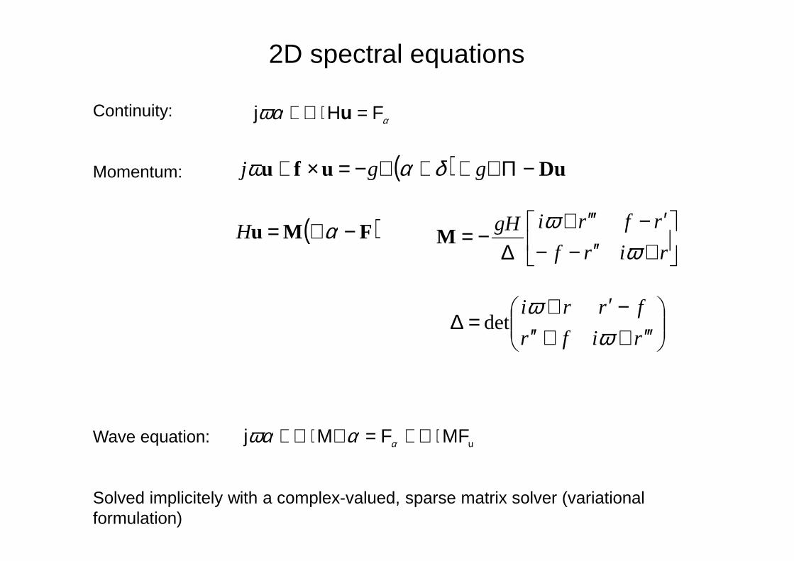
Continuity:

Momentum:

Wave equation:

Solved implicitely with a complex-valued, sparse matrix solver (variational formulation)

2D spectral equations

( ) Duufu −Π∇++∇−=×+ ggj δαω

( )FMu −∇= αH

+′′−−′−′′′+

∆−=

rirf

rfrigH

ωω

M

′′′++′′−′+

=∆rifr

frri

ωω

det

uMFFMj ⋅∇+=∇⋅∇+ ααωα

αωα FHj =⋅∇+ u

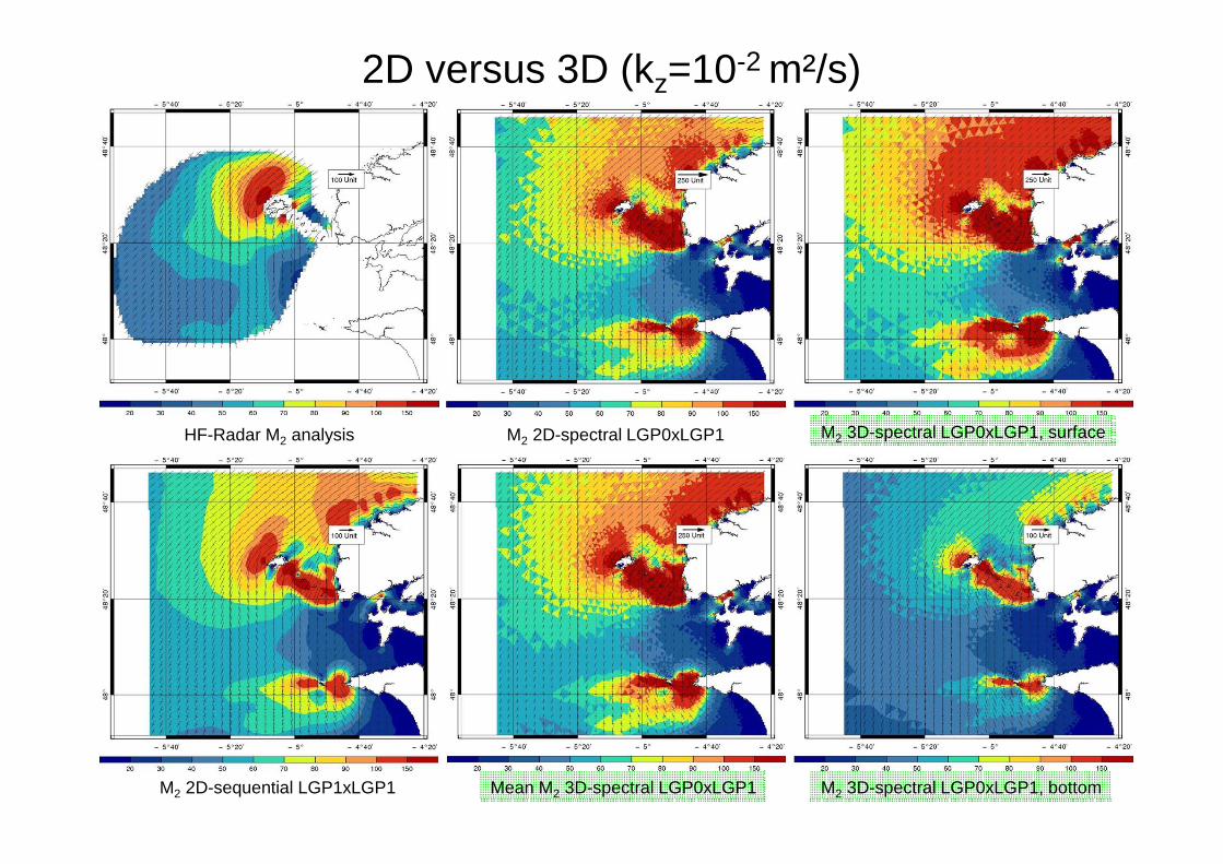
2D versus 3D (kz=10-2 m²/s)

HF-Radar M2 analysis M2 2D-spectral LGP0xLGP1

Mean M2 3D-spectral LGP0xLGP1M2 2D-sequential LGP1xLGP1 M2 3D-spectral LGP0xLGP1, bottom

M2 3D-spectral LGP0xLGP1, surface

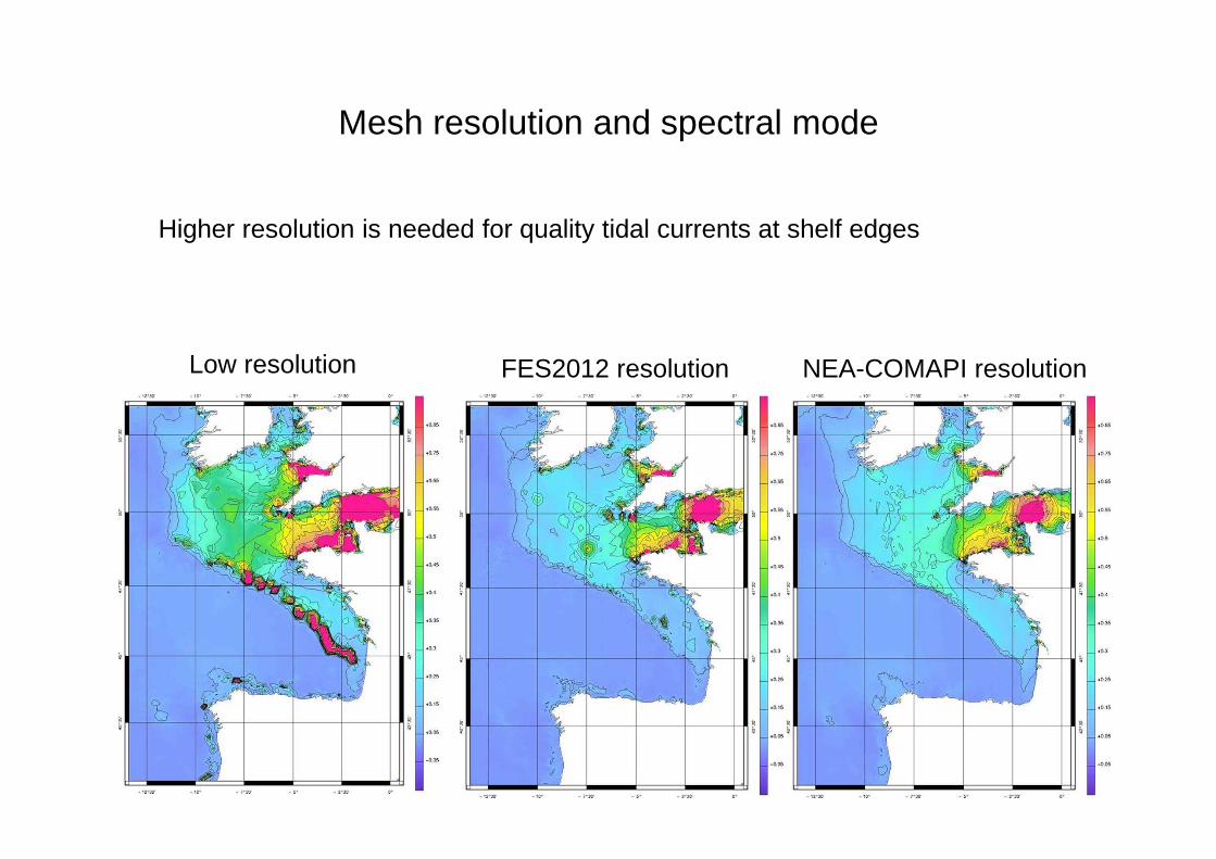
Mesh resolution and spectral mode

Higher resolution is needed for quality tidal currents at shelf edges

Low resolution FES2012 resolution NEA-COMAPI resolution

Bathymetry accuracy issue

NEA-COMAPI (optimal)

Bathymetry Version-2009

NEA (hydrodynamic)

Bathymetry Version-2010

Bathymetry Version-2009 versus XBTs depth

Bathymetry Version-2010 versus XBTs depth

M4

M2

NEA-COMAPI (hydrodynamic)

Bathymetry Version-2009

Mono-chromatic and poly-chromatic

spectral data assimilation

MICSS project (CNES/NASA foundings)P. De Mey, N. Ayoub, L. Roblou

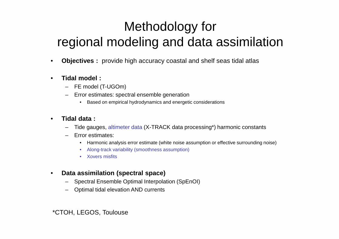
Methodology forregional modeling and data assimilation

• Objectives : provide high accuracy coastal and shelf seas tidal atlas

• Tidal model :– FE model (T-UGOm)– Error estimates: spectral ensemble generation

• Based on empirical hydrodynamics and energetic considerations

• Tidal data :– Tide gauges, altimeter data (X-TRACK data processing*) harmonic constants– Error estimates:

• Harmonic analysis error estimate (white noise assumption or effective surrounding noise)• Along-track variability (smoothness assumption)• Xovers misfits

• Data assimilation (spectral space)– Spectral Ensemble Optimal Interpolation (SpEnOI)– Optimal tidal elevation AND currents

*CTOH, LEGOS, Toulouse

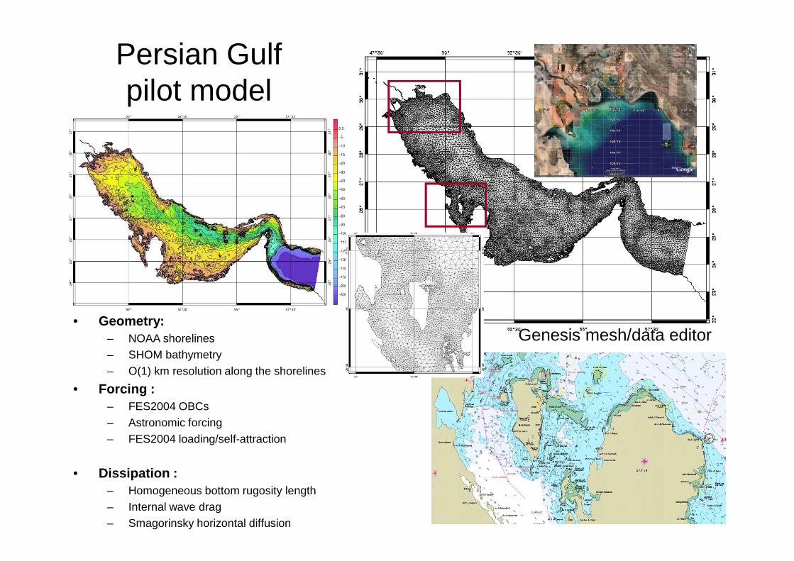
Persian Gulf pilot model

• Geometry:– NOAA shorelines– SHOM bathymetry– O(1) km resolution along the shorelines

• Forcing :– FES2004 OBCs– Astronomic forcing– FES2004 loading/self-attraction

• Dissipation :– Homogeneous bottom rugosity length– Internal wave drag– Smagorinsky horizontal diffusion

Genesis mesh/data editor

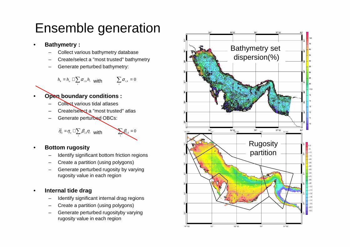
Ensemble generation• Bathymetry :

– Collect various bathymetry database– Create/select a "most trusted" bathymetry– Generate perturbed bathymetry:

with

• Open boundary conditions :– Collect various tidal atlases– Create/select a "most trusted" atlas– Generate perturbed OBCs:

with

• Bottom rugosity– Identify significant bottom friction regions– Create a partition (using polygons)– Generate perturbed rugosity by varying

rugosity value in each region

• Internal tide drag– Identify significant internal drag regions– Create a partition (using polygons)– Generate perturbed rugosityby varying

rugosity value in each region

Bathymetry set dispersion(%)

Rugositypartition

∑+=i

ikiok hhh ,α 0, =∑i

kiα

∑+=i

ikiok ηβηη ,~ 0, =∑

ikiβ

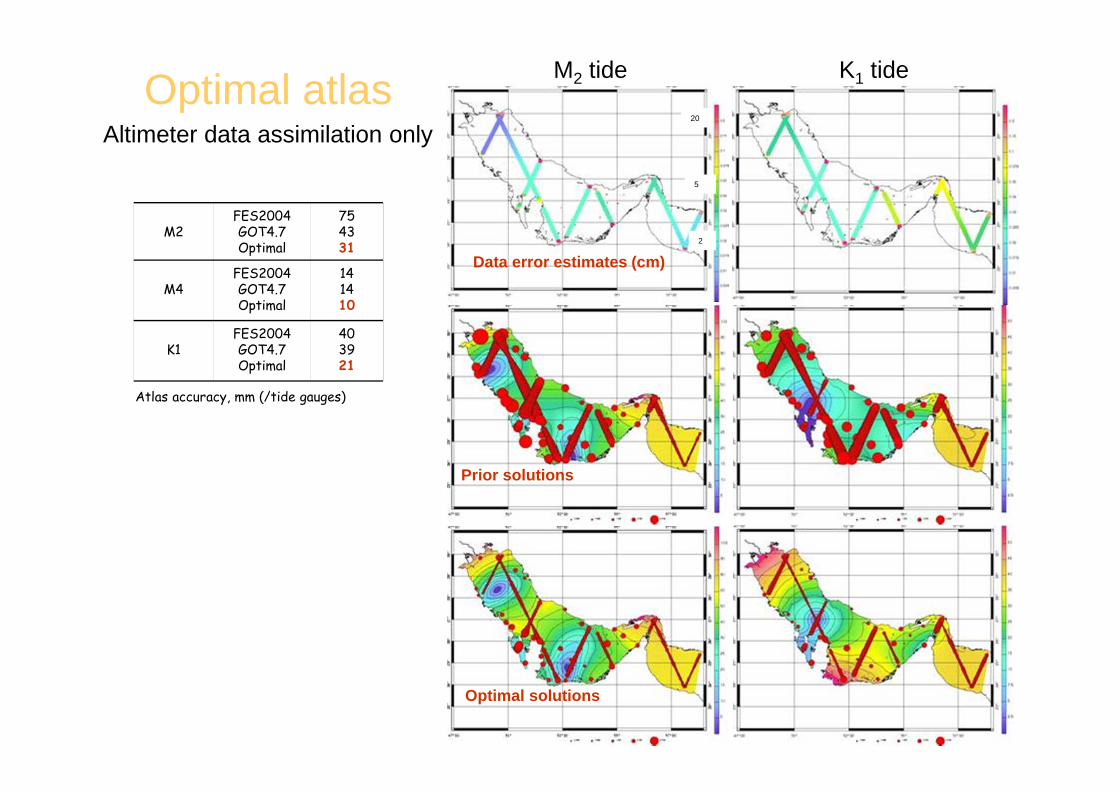
Optimal atlasM2 tide K1 tide

Altimeter data assimilation only20

2

5

M2FES2004GOT4.7Optimal

754331

M4FES2004GOT4.7Optimal

141410

K1FES2004GOT4.7Optimal

403921

Atlas accuracy, mm (/tide gauges)

Prior solutions

Optimal solutions

Data error estimates (cm)

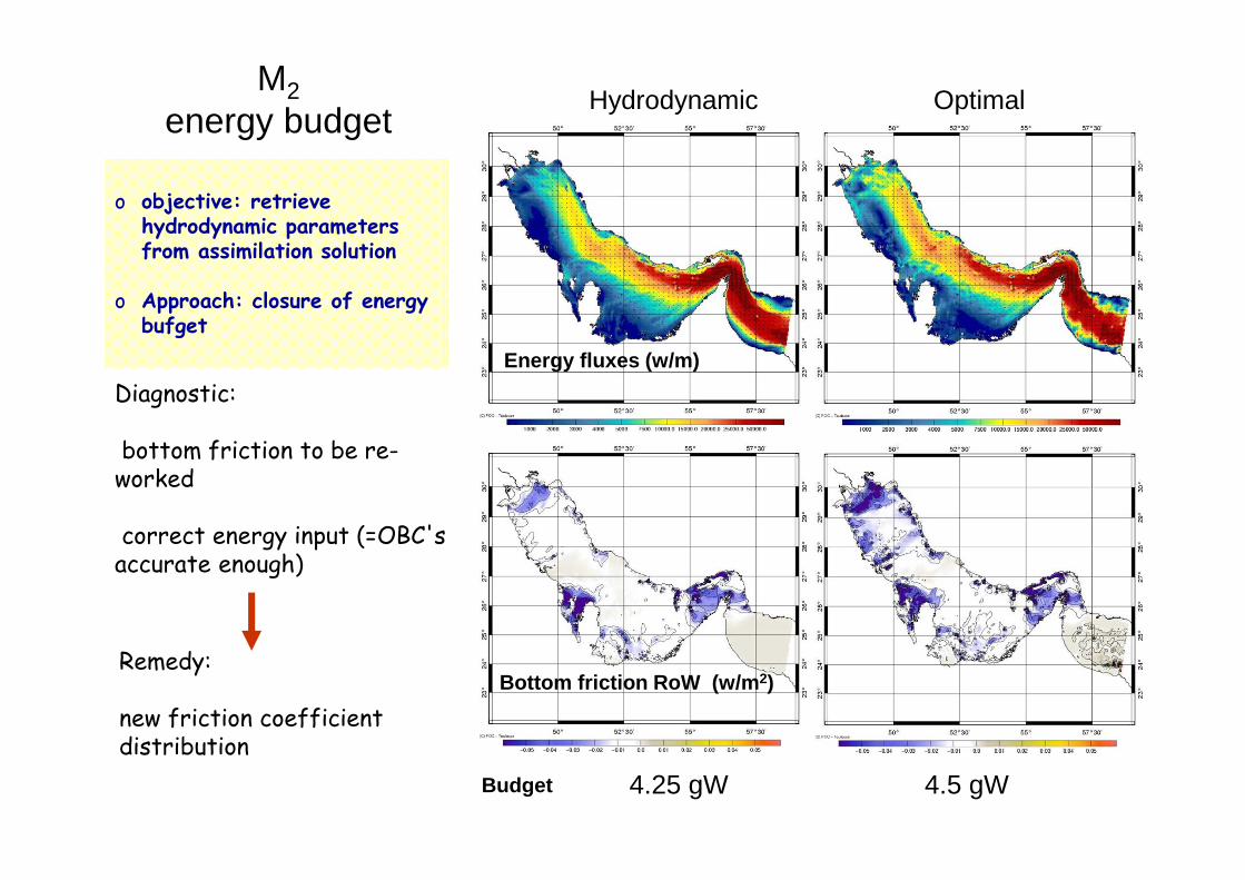
Hydrodynamic OptimalM2

energy budget

Energy fluxes (w/m)

Bottom friction RoW (w/m 2)

4.5 gW4.25 gW

o objective: retrieve hydrodynamic parameters from assimilation solution

o Approach: closure of energy bufget

Diagnostic:

bottom friction to be re-worked

correct energy input (=OBC's accurate enough)

Remedy:

new friction coefficient distribution

Budget

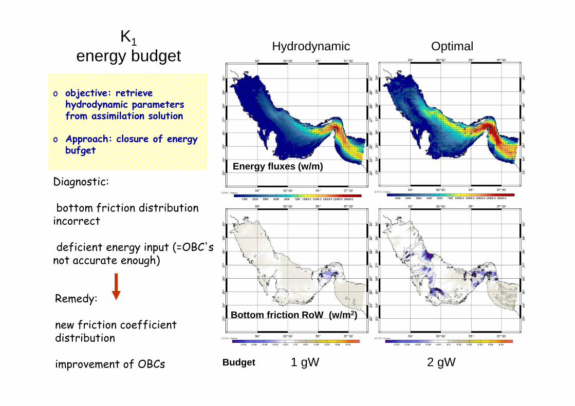
Hydrodynamic OptimalK1

energy budget

2 gW1 gW

Energy fluxes (w/m)

o objective: retrieve hydrodynamic parameters from assimilation solution

o Approach: closure of energy bufget

Diagnostic:

bottom friction distribution incorrect

deficient energy input (=OBC's not accurate enough)

Remedy:

new friction coefficient distribution

improvement of OBCs

Bottom friction RoW (w/m 2)

Budget

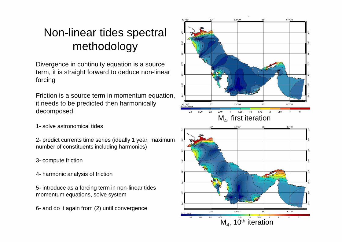
Non-linear tides spectral methodology

Divergence in continuity equation is a source term, it is straight forward to deduce non-linear forcing

Friction is a source term in momentum equation, it needs to be predicted then harmonically decomposed:

1- solve astronomical tides

2- predict currents time series (ideally 1 year, maximum number of constituents including harmonics)

3- compute friction

4- harmonic analysis of friction

5- introduce as a forcing term in non-linear tides momentum equations, solve system

6- and do it again from (2) until convergence

M4, first iteration

M4, 10th iteration

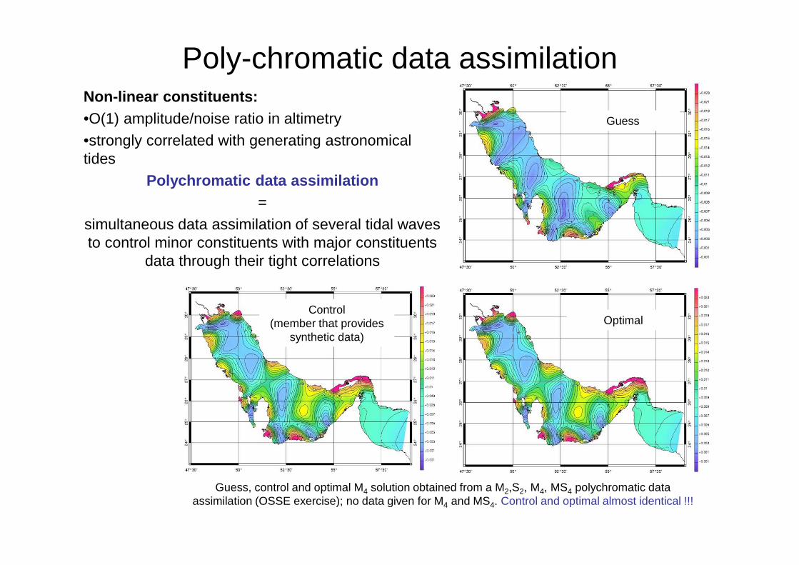
Poly-chromatic data assimilationNon-linear constituents:•O(1) amplitude/noise ratio in altimetry•strongly correlated with generating astronomical tides

Polychromatic data assimilation=

simultaneous data assimilation of several tidal waves to control minor constituents with major constituents

data through their tight correlations

Guess

Control(member that provides

synthetic data)

Optimal

Guess, control and optimal M4 solution obtained from a M2,S2, M4, MS4 polychromatic data assimilation (OSSE exercise); no data given for M4 and MS4. Control and optimal almost identical !!!