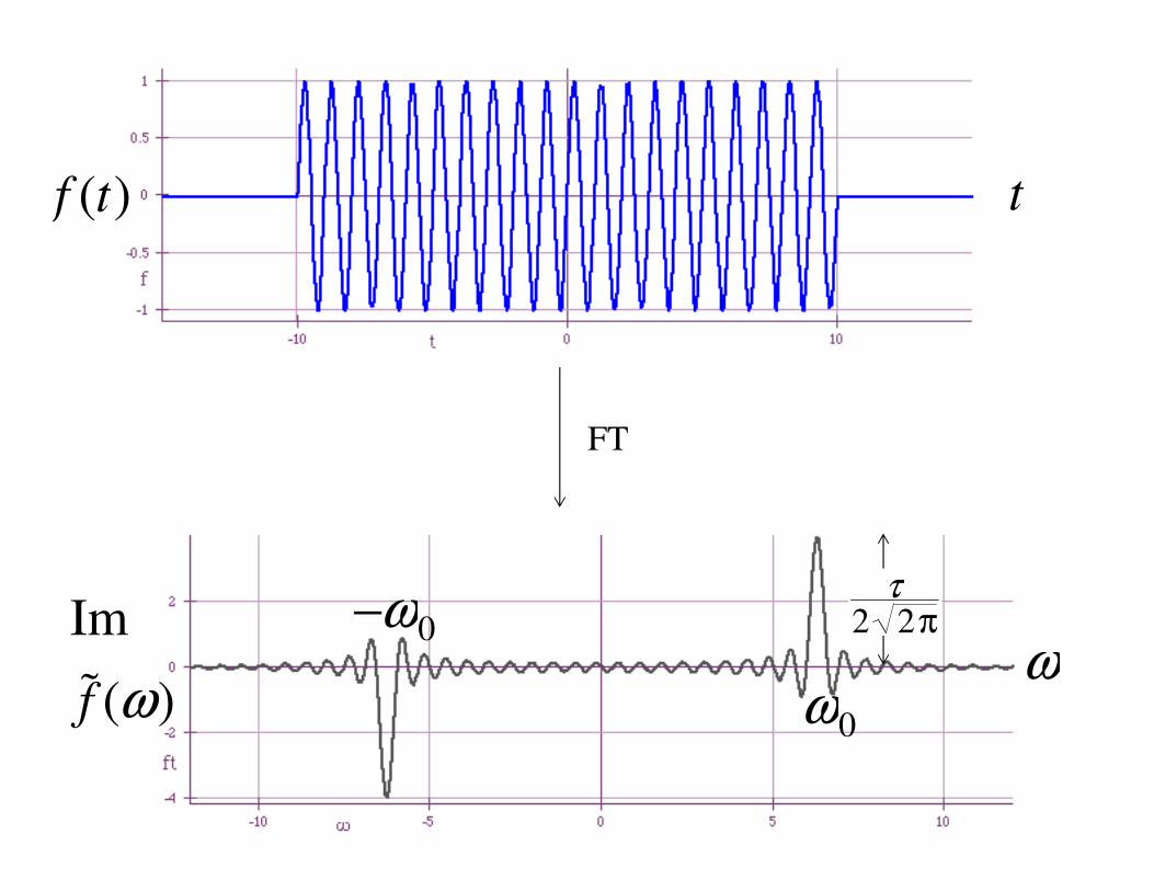
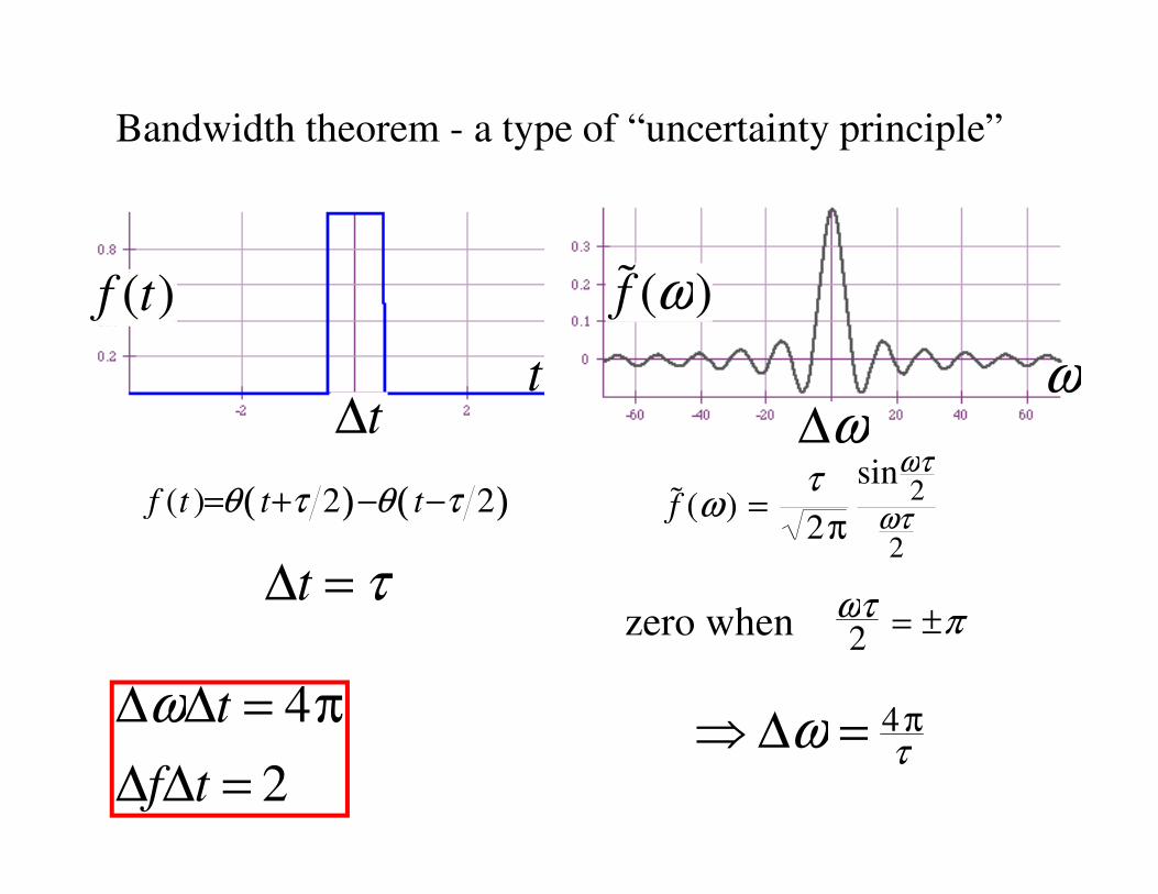
Bandwidth theorem - a type of “uncertainty principle”

f (t)

t∆t

f (t )=θ t+τ 2( )−θ t−τ 2( )

˜ f (ω)

ω∆ω

˜ f (ω ) =τ

2π

sinωτ2

ωτ2

ωτ2

= ±πzero when

⇒ ∆ω = 4πτ

∆t = τ

∆ω∆t = 4π

∆f∆t = 2

Reading:

Taylor 5.8

Main 11.3

Riley 13.1

THE DRIVEN LRC CIRCUIT

(A special driving function that is an impulse

function)

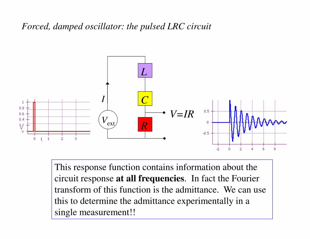
Forced, damped oscillator: the pulsed LRC circuit

L

R

CI

Vext

V=IR

This response function contains information about the

circuit response at all frequencies. In fact the Fourier

transform of this function is the admittance. We can use

this to determine the admittance experimentally in a

single measurement!!

A few words before we begin. We can actually calculate the time response of a series

LRC circuit to a delta function driving force rather easily without resorting to Fourier

analysis (and we will, later). But the impulse function is very special, and with other,

more general driving functions, the Fourier approach is much easier.

You might object - the impulse function “drives” the circuit for only a very short time

and the rest of the time, the circuit is “free”. Is this really a driving force? Well, yes,

it is. That voltage application for a short time is important.

You might object more - the impulse function is not a periodic function - how can it

be represented by a Fourier series, then? This is only a minor problem. You can think

of a non-periodic function as a periodic function with an extremely long period. The

concept is the same. In the lab, you will actually drive the circuit with a “periodic

impulse function”: an impulse is applied, then another a long time later, and then

another along time after that, and so on.

Another objection - the data you acquire in the lab for the current in the “driven”

circuit as a function of time is not continuous. How will you find the Fourier

spectrum of a discrete function? This again is not a problem of principle. We simply

need some numeric techniques - the technique is the FFT, the fast Fourier transform.

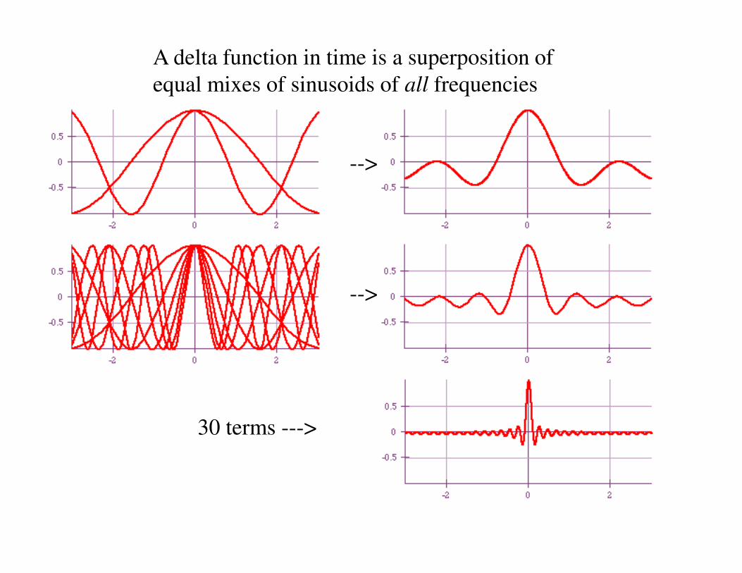
30 terms --->

A delta function in time is a superposition of

equal mixes of sinusoids of all frequencies

-->

-->

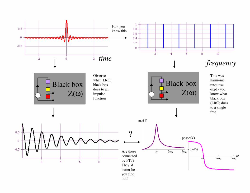
timefrequency

?

This was

harmonic

response

expt - you

know what

black box

(LRC) does

to a single

freq

Observe

what (LRC)

black box

does to an

impulse

function

FT - you

know this

Are these

connected

by FT??

They’d

better be -

you find

out!

Black box

Z(ω)

Black box

Z(ω)

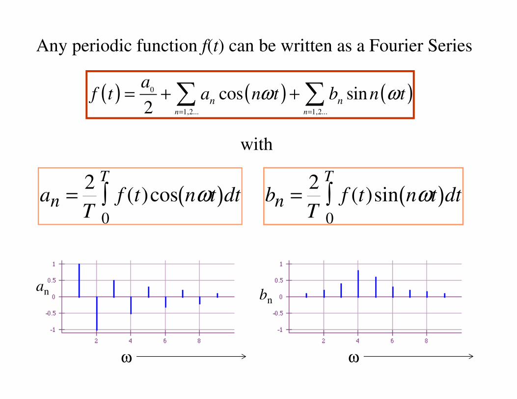
Any periodic function f(t) can be written as a Fourier Series

f t( ) =a

0

2+ an cos nωt( )

n=1,2...

∑ + bn sinn ωt( )n=1,2...

∑

with

an =2

Tf (t)cos nωt( )dt

0

T

∫ bn =2

Tf (t)sin nωt( )dt

0

T

∫

ω

an

ω

bn

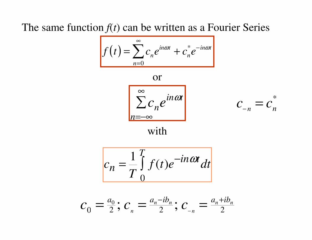
The same function f(t) can be written as a Fourier Series

f t( ) = cneinωt

+ cn

*e

− inωt

n=0

∞

∑

or

cneinωt

n=−∞

∞

∑

with

cn =1

Tf (t)e−inωt

dt0

T

∫

c0 =a0

2 ; cn=

an −ibn

2 ; c−n

=an +ibn

2

c−n

= cn

*

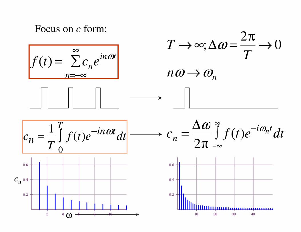
Focus on c form:

f (t) = cneinωt

n=−∞

∞

∑

cn =1

Tf (t)e−inωt

dt0

T

∫

T → ∞;∆ω =2π

T→ 0

nω → ωn

cn =∆ω

2πf (t)e−iωnt

dt−∞

∞

∫

ω

cn

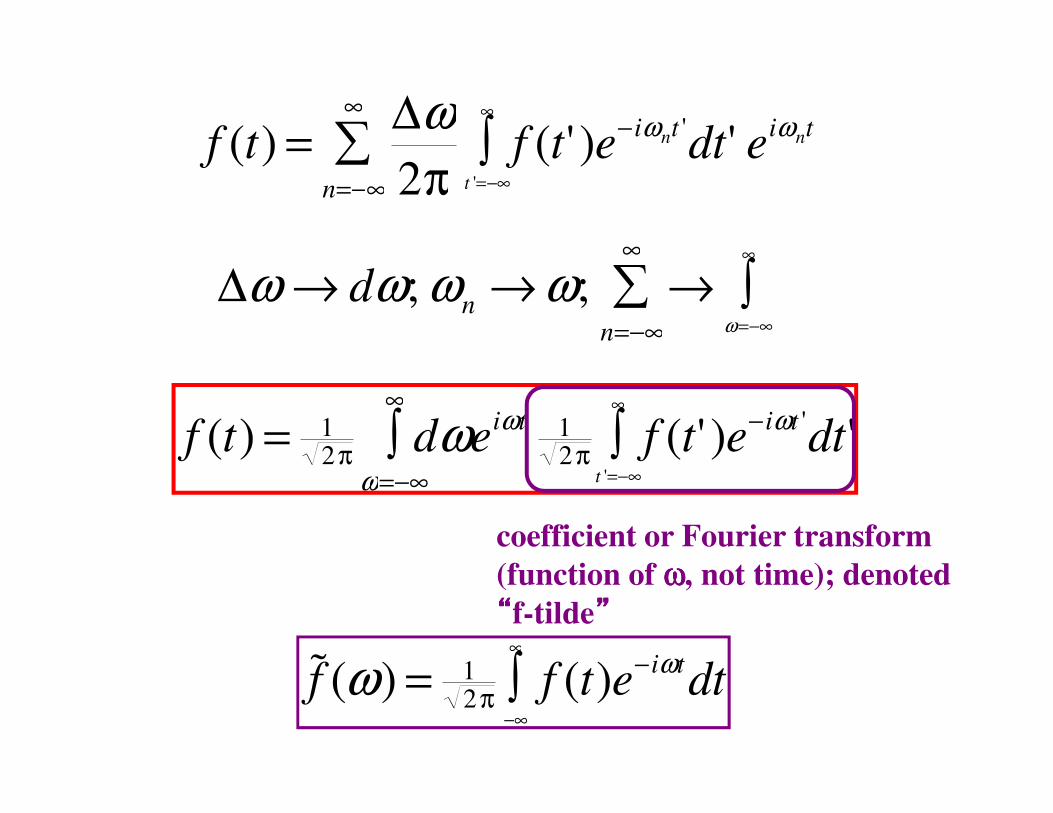
f (t) =∆ω

2πf (t' )e−iωnt '

dtt '=−∞

∞

∫ ' eiωnt

n=−∞

∞

∑

f (t) = 12π

dωeiωt 1

2πω=−∞

∞

∫ f (t' )e−iωt 'dt

t '=−∞

∞

∫ '

∆ω → dω; ωn

→ ω; →ω=−∞

∞

∫n=−∞

∞

∑

coefficient or Fourier transform

(function of ωωωω, not time); denoted

““““f-tilde””””

˜ f (ω) = 12π

f (t)e−iωtdt

−∞

∞

∫

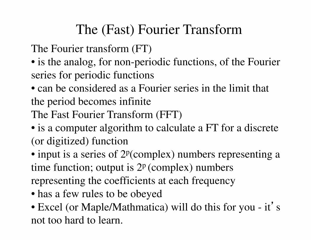
The (Fast) Fourier Transform

The Fourier transform (FT)

• is the analog, for non-periodic functions, of the Fourier

series for periodic functions

• can be considered as a Fourier series in the limit that

the period becomes infinite

The Fast Fourier Transform (FFT)

• is a computer algorithm to calculate a FT for a discrete

(or digitized) function

• input is a series of 2p(complex) numbers representing a

time function; output is 2p (complex) numbers

representing the coefficients at each frequency

• has a few rules to be obeyed

• Excel (or Maple/Mathmatica) will do this for you - it’s

not too hard to learn.

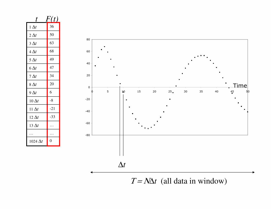
-80

-60

-40

-20

0

20

40

60

80

0 5 10 15 20 25 30 35 40 45 50

Time

1 ∆t 36

2 ∆t 50

3 ∆t 63

4 ∆t 68

5 ∆t 49

6 ∆t 47

7 ∆t 34

8 ∆t 20

9 ∆t 6

10 ∆t -8

11 ∆t -21

12 ∆t -33

13 ∆t …

… …

1024 ∆t 0

∆t

Τ = Ν∆t (all data in window)

t F(t)

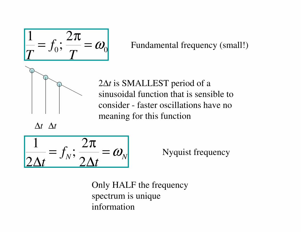
1

T= f0;

2π

T= ω0

Fundamental frequency (small!)

∆t ∆t

2∆t is SMALLEST period of a

sinusoidal function that is sensible to

consider - faster oscillations have no

meaning for this function

1

2∆t= f

N;

2π

2∆t= ω

NNyquist frequency

Only HALF the frequency

spectrum is unique

information

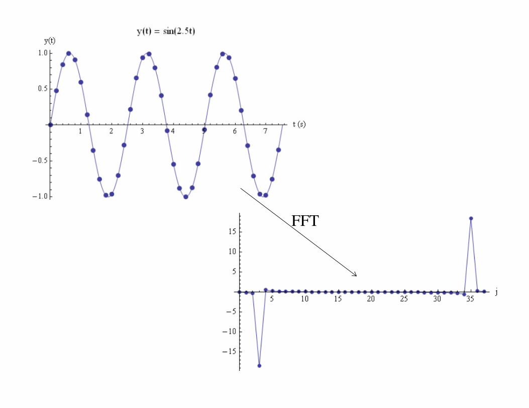
FFT

f (t) t

Im

˜ f (ω) ω0

−ω0ω

τ2 2π

FT

-0.5

0

0.5

y

2 4x

-0.5

0

0.5

2 4

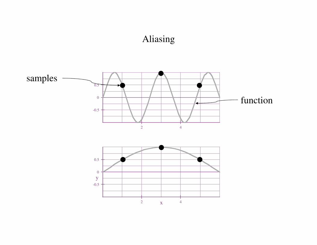
samples

function

Aliasing

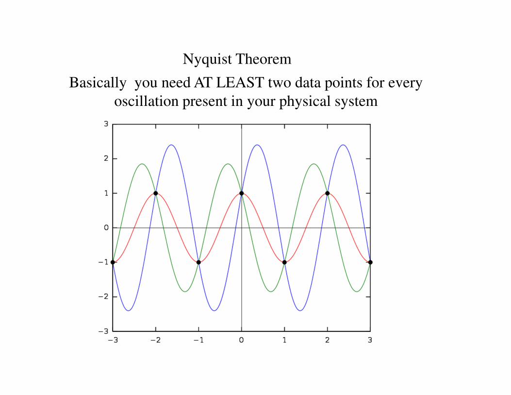
Nyquist Theorem

Basically you need AT LEAST two data points for every

oscillation present in your physical system

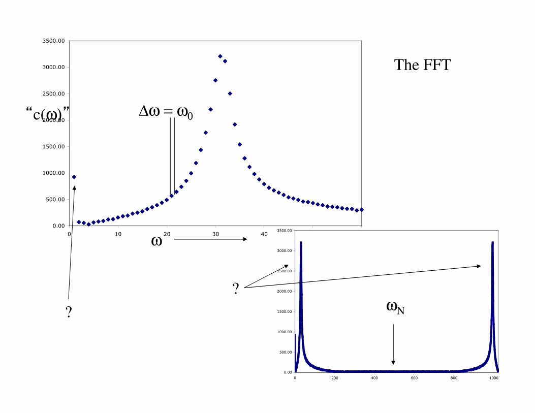
0.00

500.00

1000.00

1500.00

2000.00

2500.00

3000.00

3500.00

0 10 20 30 40 50 60

∆ω = ω0

ω

“c(ω)”

0.00

500.00

1000.00

1500.00

2000.00

2500.00

3000.00

3500.00

0 200 400 600 800 1000

ωΝ

The FFT

?

?

Plan:

The “Fourier representation” for a non-periodic function like a

delta function is the Fourier transform - it’s really a Fourier

series but with a very (infinitely) small fundamental

frequency. We’ll talk about this, and do some analytical

examples later.

If we want the Fourier transform of an experimentally

measured (i.e. digitized) function, we have to do something

called a Fast Fourier Transform (FFT). Excel or Maple will

help here, but we have to understand a few things about this.

Once we understand the concept of the FT and the FFT, we’ll

experimentally measure the response of the same LRC circuit

to an impulse (delta) function. We’ll FFT the response

function, and discuss what we find.

Plan cont’d:

Once we’ve done this experiment, we’ll go back and do some

analytical examples of Fourier transforms, and in particular,

we’ll FT (analytically now) the damped harmonic oscillator

response and show analytically that it really is the admittance

function.

We also want to know how to calculate the time response of

the LRC circuit to an arbitrary waveform, without using the

easier Fourier route. We’ll calculate the response to a delta

function (impulse) which we already measured so we have a

good idea of what to expect. Then we’ll use superposition to

add up a number of sequential delta functions, and find the

total response.

Finally, we’ll FT the expression for the general time response

and we’ll discover the admittance function again.