T P tt Δt - acclab.helsinki.fiknordlun/moldyn/lecture11.pdf · SR. to describe repulsion ......

Set the initial conditions , ri t0( ) vi t0( )

Get new forces Fi ri( )

Solve the equations of motion numerically over time step :

Δtri tn( ) ri tn 1+( )→ vi tn( ) vi tn 1+( )→

t t Δt+→

Get desired physical quantities

t tmax ?> Calculate results and finish

Update neighborlist

Perform , scaling (ensembles)T P

Potential models ionic compounds

Introduction to molecular dynamics 2015 11. Potential models for ionic compounds 1

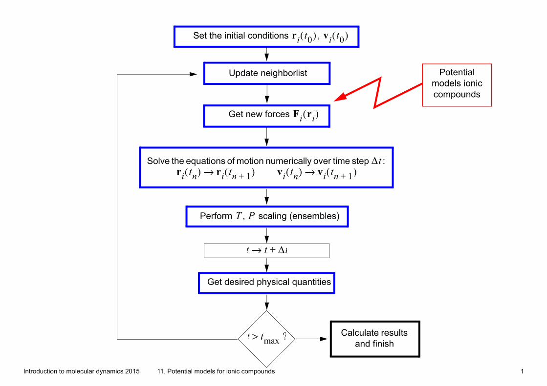
Potentials for ionic compounds• There is a wide range of materials where ionic interactions are important:

• In hard condensed matter many, if not most, compounds have at least some degree of ionicity.• Partial ionic charges are also very important for organic materials

• In ionic compounds one can simply describe the long-range interaction with a Coulomb pair potential. But one should add a short-range interaction VSR to describe repulsion at short dis-

tances:

V rij( ) VSR rij( )z1z2e2

4πε0rij------------------+= ;

• The charges zi are often fractional charges, depending on the degree of ionicity of a material (e.g. NaCl:

1, GaN: 0.5, GaAs: 0.2, Si 0.0).

• VSR contains the repulsion of the electron shells and possibly an attractive van der Waals-interaction.

Common forms:

• Buckingham: VSR r( ) Ae r ρ/– C

r6-----–=

• Born-Huggins-Mayer: VSR r( ) Ae B r σ–( )– C

r6----- D

r8-----––=

• Morse: VSR r( ) De 2α r r0–( )– 2De α r r0–( )––=


Potentials for ionic compounds• The repulsion is usually significant only for nearest neighbours, and the van der Waals interac-

tion for the 2-nd neighbours. In oxides frequently the interaction between cations is assumed to be only the Coulomb repulsion.

• In many real compounds the interactions are a mixture of covalent, metallic and ionic interac-tions (e.g. many carbides and nitrodes).


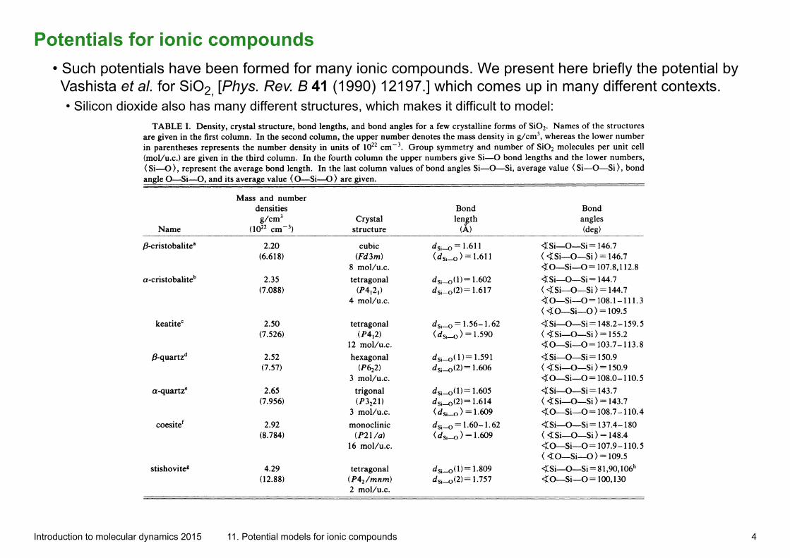
Potentials for ionic compounds• Such potentials have been formed for many ionic compounds. We present here briefly the potential by Vashista et al. for SiO2, [Phys. Rev. B 41 (1990) 12197.] which comes up in many different contexts.• Silicon dioxide also has many different structures, which makes it difficult to model:


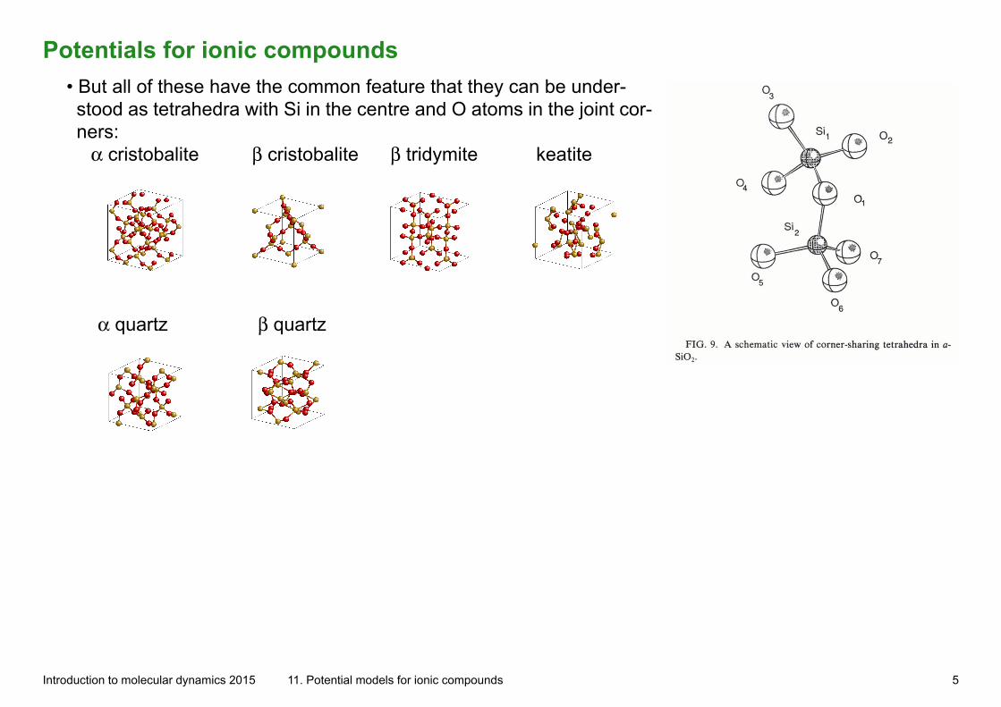
Potentials for ionic compounds• But all of these have the common feature that they can be under-stood as tetrahedra with Si in the centre and O atoms in the joint cor-ners: α cristobalite β cristobalite β tridymite keatite

α quartz β quartz


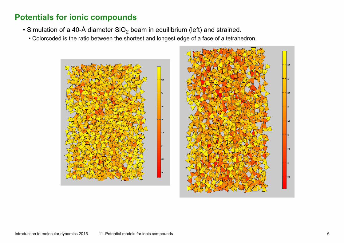
Potentials for ionic compounds• Simulation of a 40-Å diameter SiO2 beam in equilibrium (left) and strained.

• Colorcoded is the ratio between the shortest and longest edge of a face of a tetrahedron.


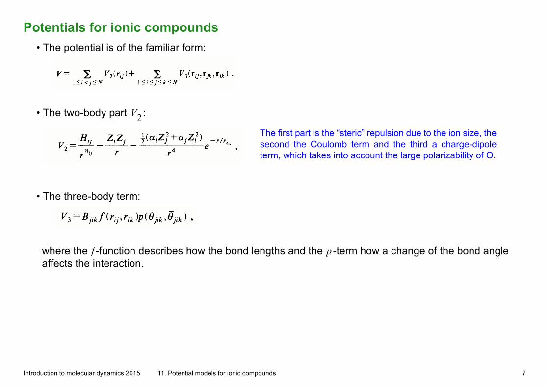
Potentials for ionic compounds• The potential is of the familiar form:

• The two-body part V2 :

The first part is the “steric” repulsion due to the ion size, the second the Coulomb term and the third a charge-dipole term, which takes into account the large polarizability of O.

• The three-body term:

where the f -function describes how the bond lengths and the p -term how a change of the bond angle affects the interaction.


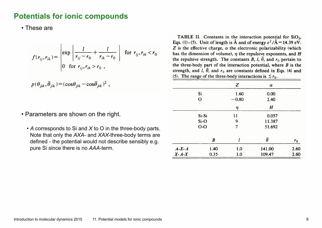
Potentials for ionic compounds• These are

• Parameters are shown on the right.

• A corresponds to Si and X to O in the three-body parts. Note that only the AXA- and XAX-three-body terms are defined - the potential would not describe sensibly e.g. pure Si since there is no AAA-term.


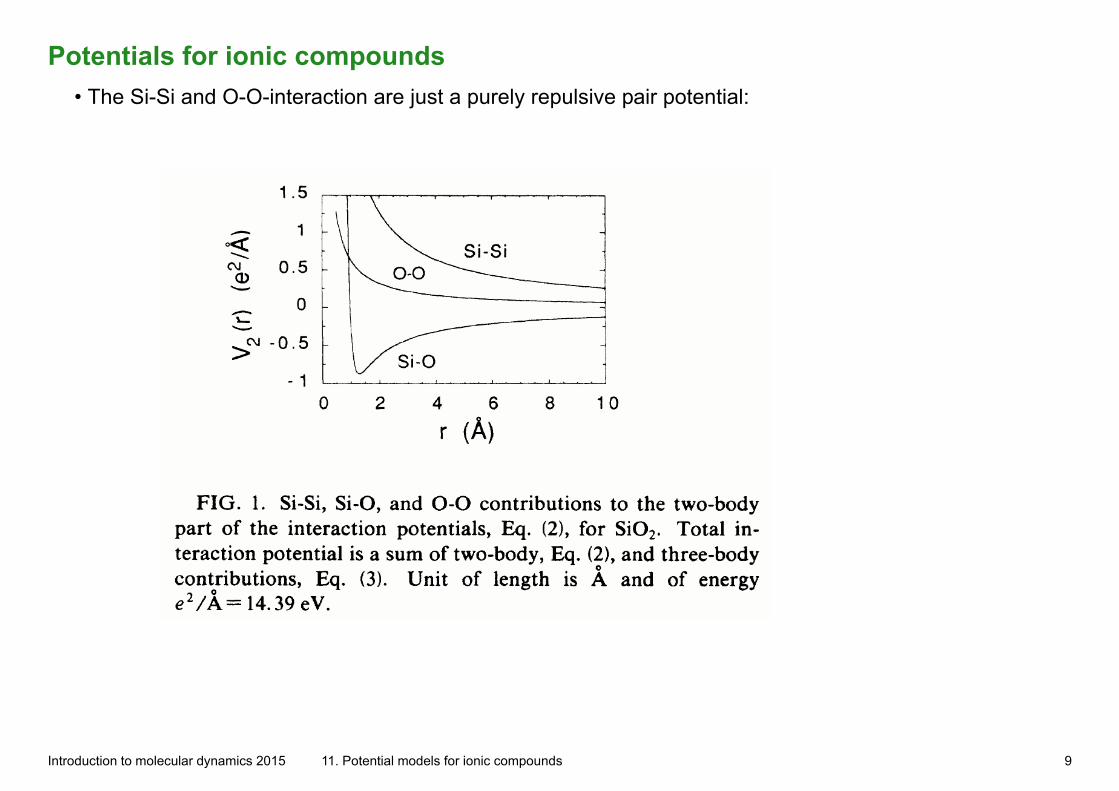
Potentials for ionic compounds• The Si-Si and O-O-interaction are just a purely repulsive pair potential:


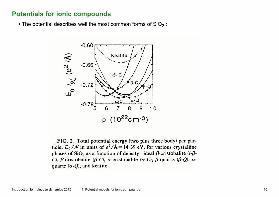
Potentials for ionic compounds• The potential describes well the most common forms of SiO2 :


Potentials for ionic compounds• A newer potential was developed by Watanabe et al. [Appl. Surf. Sci. 234 (2004) 207.].

• One of its strengths is the ability to describe also the so called sub-oxides of SiO2; e.g. SiO.

• Because of this it is suitable for describing interfaces between Si and SiO2 and to be used in defect studies and ion

bombardment simulations.• The potential is based on the Stillinger-Weber potential and the Si-Si interaction is the original Si-SW.

• Examples of its use in nanocluster bombardment can be found in J. Samela’s PhD thesis1.• However, its elastic properties are not very good, strongly overestimates e.g. bulk modulus

• An SiO2 potential in the Tersoff formalism: [Munetoh et al, Comput. Mater. Sci. 39 (2007) 334]: better than Watanabe in some elastic and melting properties

1. Electronically available at http://urn.fi/URN:ISBN:978-952-10-3927-0


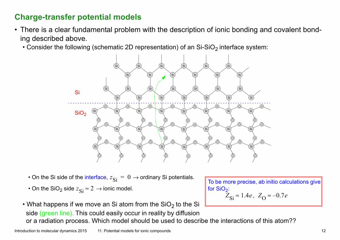
Charge-transfer potential models• There is a clear fundamental problem with the description of ionic bonding and covalent bond-

ing described above. • Consider the following (schematic 2D representation) of an Si-SiO2 interface system:

Si

Si

Si

Si

Si

Si

Si

Si

Si

Si

Si

Si

Si

Si

Si

Si

Si

Si

Si

Si

Si

Si

Si

Si

Si

Si

Si

O

O

Si

O

O

Si

O

O

Si

O

O

Si

O

O

Si

O

O

Si

O

O

Si

O

O

Si

O

O

Si

O

O

Si

O

O

Si

O

O

Si

O

O

Si

O

O

Si

O

O

Si

O

O

Si

O

O

Si

O

O

Si

O

O

Si

O

O

Si

O

O

Si

O

O

Si

O

O

Si

O

O

Si

SiO2

• On the Si side of the interface, zSi 0= → ordinary Si potentials. To be more precise, ab initio calculations give for SiO2:

, ZSi 1.4e≈ ZO 0.7e–≈• On the SiO2 side zSi 2≈ → ionic model.

• What happens if we move an Si atom from the SiO2 to the Si side (green line). This could easily occur in reality by diffusion or a radiation process. Which model should be used to describe the interactions of this atom??


Charge-transfer potential models• Here we get to the charge transfer model for the atoms, where the environment-dependence of

the ionicity of the atom is built into the model.

• There are extremely few models like this, since charge transfer processes are difficult to deal with and poorly understood.

• One fairly well motivated approach is that of Alavi et al., Phil. Mag. B 65 (1992) 489.

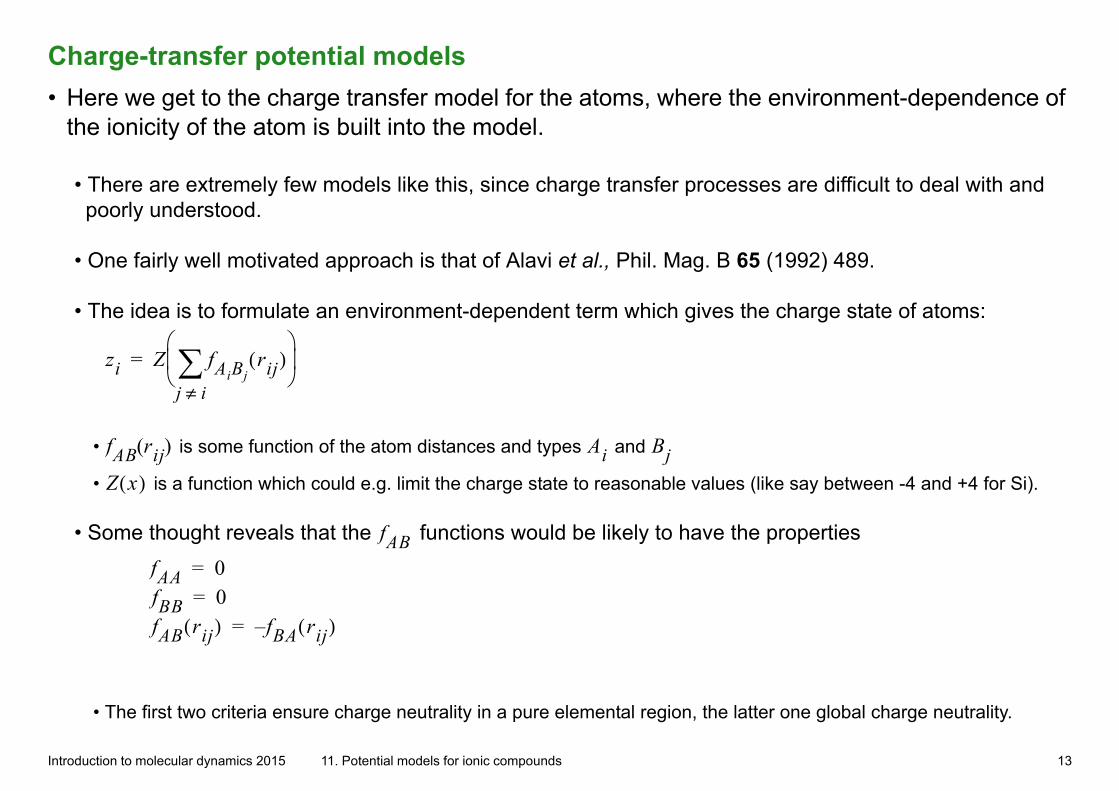
• The idea is to formulate an environment-dependent term which gives the charge state of atoms:

zi Z fAiBjrij( )

j i≠

=

• fAB rij( ) is some function of the atom distances and types Ai and Bj

• Z x( ) is a function which could e.g. limit the charge state to reasonable values (like say between -4 and +4 for Si).

• Some thought reveals that the fAB functions would be likely to have the properties

fAA 0fBB 0fAB rij( ) f– BA rij( )

==

=

• The first two criteria ensure charge neutrality in a pure elemental region, the latter one global charge neutrality.


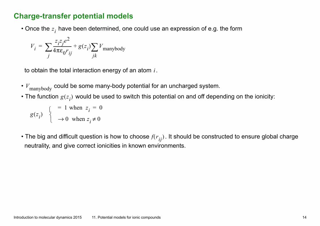
Charge-transfer potential models• Once the zi have been determined, one could use an expression of e.g. the form

Vi

zizje2

4πε0rij------------------

j g zi( ) Vmanybody

jk+=

to obtain the total interaction energy of an atom i .

• Vmanybody could be some many-body potential for an uncharged system.

• The function g zi( ) would be used to switch this potential on and off depending on the ionicity:

g zi( ) 1= when zi 0=

0→ when zi 0≠

• The big and difficult question is how to choose f rij( ) . It should be constructed to ensure global charge

neutrality, and give correct ionicities in known environments.


Charge-transfer potential models

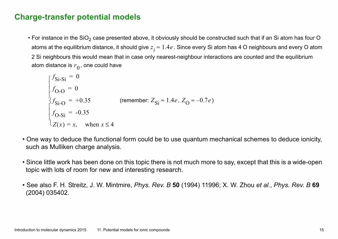
• For instance in the SiO2 case presented above, it obviously should be constructed such that if an Si atom has four O

atoms at the equilibrium distance, it should give zi 1.4e≈ . Since every Si atom has 4 O neighbours and every O atom

2 Si neighbours this would mean that in case only nearest-neighbour interactions are counted and the equilibrium

atom distance is r0 , one could have

fSi-Si 0=

fO-O 0=

fSi-O +0.35=

fO-Si -0.35=

Z x( ) x= when x 4≤,

(remember: ZSi 1.4e≈ , ZO 0.7e–≈ )

• One way to deduce the functional form could be to use quantum mechanical schemes to deduce ionicity, such as Mulliken charge analysis.

• Since little work has been done on this topic there is not much more to say, except that this is a wide-open topic with lots of room for new and interesting research.

• See also F. H. Streitz, J. W. Mintmire, Phys. Rev. B 50 (1994) 11996; X. W. Zhou et al., Phys. Rev. B 69 (2004) 035402.


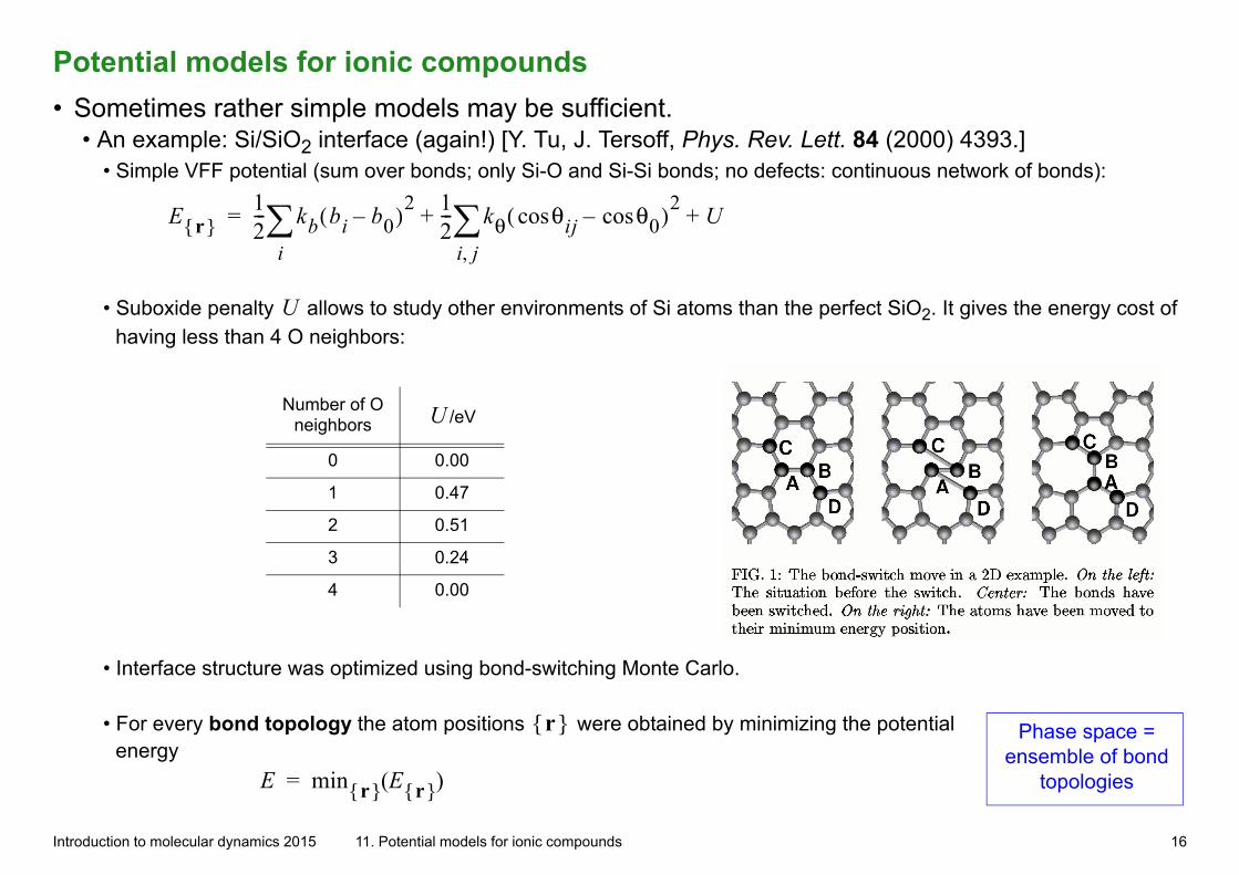
Potential models for ionic compounds• Sometimes rather simple models may be sufficient.

• An example: Si/SiO2 interface (again!) [Y. Tu, J. Tersoff, Phys. Rev. Lett. 84 (2000) 4393.]• Simple VFF potential (sum over bonds; only Si-O and Si-Si bonds; no defects: continuous network of bonds):

E r{ }12--- kb bi b0–( )2

i

12--- kθ θijcos θ0cos–( )2

i j, U+ +=

• Suboxide penalty U allows to study other environments of Si atoms than the perfect SiO2. It gives the energy cost of

having less than 4 O neighbors:

Number of O neighbors /eV

0 0.00

1 0.47

2 0.51

3 0.24

4 0.00

U

• Interface structure was optimized using bond-switching Monte Carlo.

• For every bond topology the atom positions r{ } were obtained by minimizing the potential energy

Phase space = ensemble of bond

topologies

E min r{ } E r{ }( )=


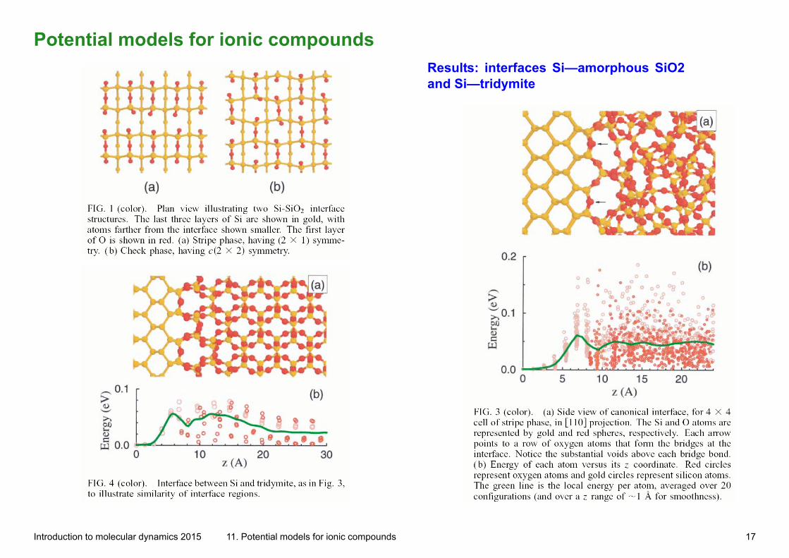
Potential models for ionic compounds

Results: interfaces Si—amorphous SiO2 and Si—tridymite

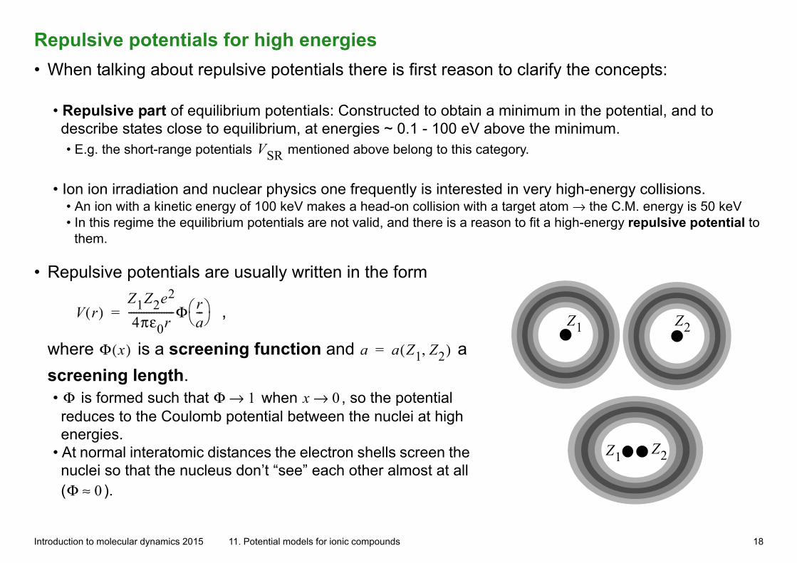
Repulsive potentials for high energies• When talking about repulsive potentials there is first reason to clarify the concepts:

• Repulsive part of equilibrium potentials: Constructed to obtain a minimum in the potential, and to describe states close to equilibrium, at energies ~ 0.1 - 100 eV above the minimum. • E.g. the short-range potentials VSR mentioned above belong to this category.

• Ion ion irradiation and nuclear physics one frequently is interested in very high-energy collisions. • An ion with a kinetic energy of 100 keV makes a head-on collision with a target atom → the C.M. energy is 50 keV • In this regime the equilibrium potentials are not valid, and there is a reason to fit a high-energy repulsive potential to

them.

• Repulsive potentials are usually written in the form

V r( )Z1Z2e2

4πε0r------------------Φ r

a--- = , Z1 Z2

Z1 Z2

where Φ x( ) is a screening function and a a Z1 Z2,( )= a

screening length. • Φ is formed such that Φ 1→ when x 0→ , so the potential reduces to the Coulomb potential between the nuclei at high energies.

• At normal interatomic distances the electron shells screen the nuclei so that the nucleus don’t “see” each other almost at all (Φ 0≈ ).


Repulsive potentials for high energies• At very small distances the nuclei are so close that the electron clouds do not screen them. The interac-tion is then purely Coulombic and Φ 1≈ .

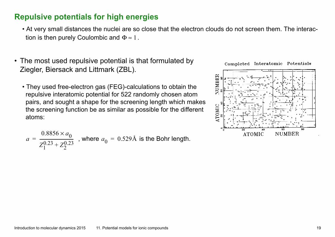
• The most used repulsive potential is that formulated by Ziegler, Biersack and Littmark (ZBL).

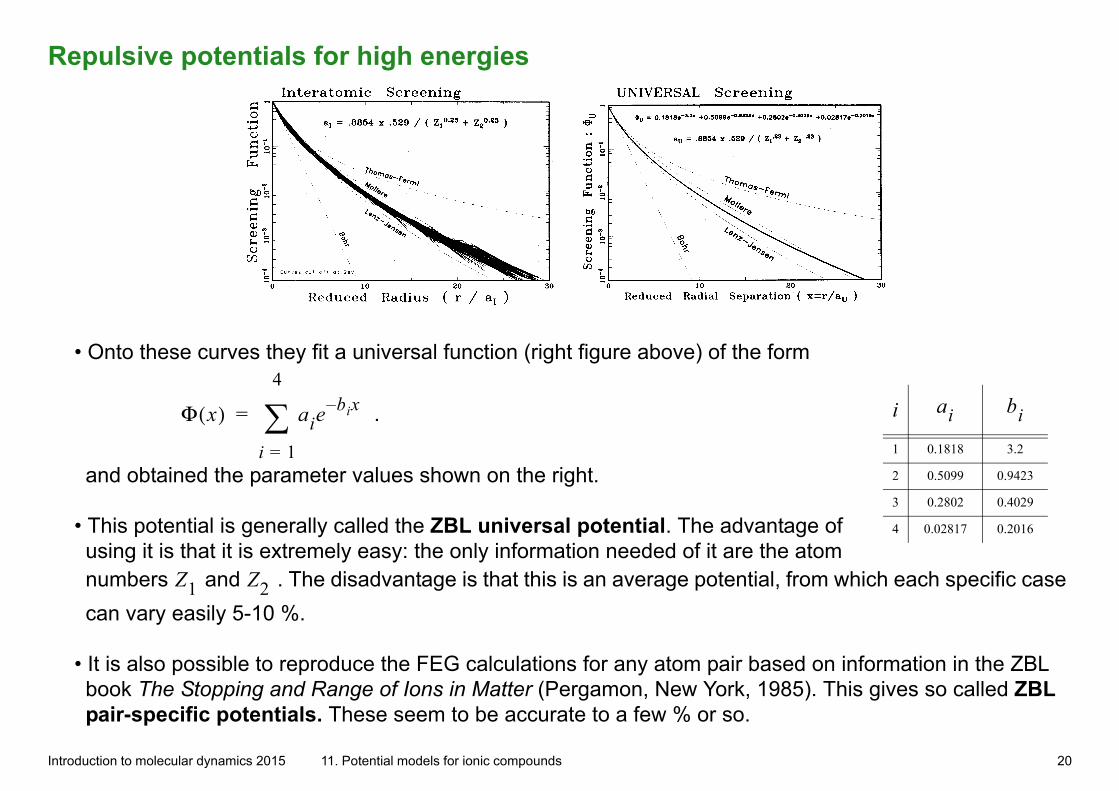
• They used free-electron gas (FEG)-calculations to obtain the repulsive interatomic potential for 522 randomly chosen atom pairs, and sought a shape for the screening length which makes the screening function be as similar as possible for the different atoms:

a0.8856 a0×

Z10.23 Z2

0.23+--------------------------------= , where a0 0.529Å= is the Bohr length.


Repulsive potentials for high energies

• Onto these curves they fit a universal function (right figure above) of the form

Φ x( ) aiebix–

i 1=

4

= .

1 0.1818 3.2

2 0.5099 0.9423

3 0.2802 0.4029

4 0.02817 0.2016

i ai bi

and obtained the parameter values shown on the right.

• This potential is generally called the ZBL universal potential. The advantage of using it is that it is extremely easy: the only information needed of it are the atom numbers Z1 and Z2 . The disadvantage is that this is an average potential, from which each specific case

can vary easily 5-10 %.

• It is also possible to reproduce the FEG calculations for any atom pair based on information in the ZBL book The Stopping and Range of Ions in Matter (Pergamon, New York, 1985). This gives so called ZBL pair-specific potentials. These seem to be accurate to a few % or so.


Repulsive potentials for high energies

• In case the best possible accuracy is desired, one can use Hartree-Fock- or DFT-calculations of the energy of a dimer, or even better an atom inside a solid.

• With dimer calculations by using certain HF- , HFS- and DFT methods it is possible to obtain the high-energy repulsive potential to ~ 1 % accuracy [Nordlund, Runeberg and Sundholm, Nucl. Instr. Meth. Phys. Res. B 132 (1997) 45].


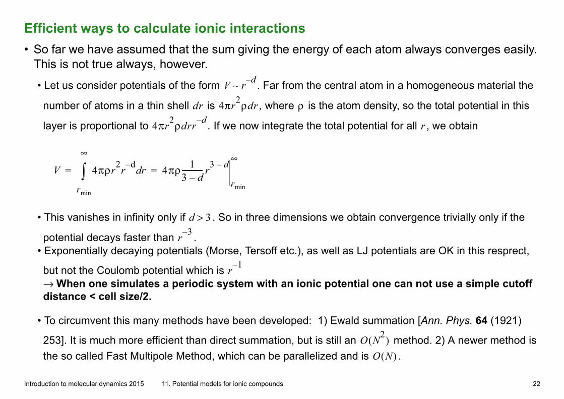
Efficient ways to calculate ionic interactions• So far we have assumed that the sum giving the energy of each atom always converges easily.

This is not true always, however.

• Let us consider potentials of the form V rd–∼ . Far from the central atom in a homogeneous material the

number of atoms in a thin shell dr is 4πr2ρdr , where ρ is the atom density, so the total potential in this

layer is proportional to 4πr2ρdrr

d–. If we now integrate the total potential for all r , we obtain

V 4πρr2r

d–rd

rmin

∞

4πρ 13 d–------------ r

3 d–

rmin

∞= =

• This vanishes in infinity only if d 3> . So in three dimensions we obtain convergence trivially only if the

potential decays faster than r3–

. • Exponentially decaying potentials (Morse, Tersoff etc.), as well as LJ potentials are OK in this resprect,

but not the Coulomb potential which is r1–

→ When one simulates a periodic system with an ionic potential one can not use a simple cutoff distance < cell size/2.

• To circumvent this many methods have been developed: 1) Ewald summation [Ann. Phys. 64 (1921)

253]. It is much more efficient than direct summation, but is still an O N2( ) method. 2) A newer method is

the so called Fast Multipole Method, which can be parallelized and is O N( ) .


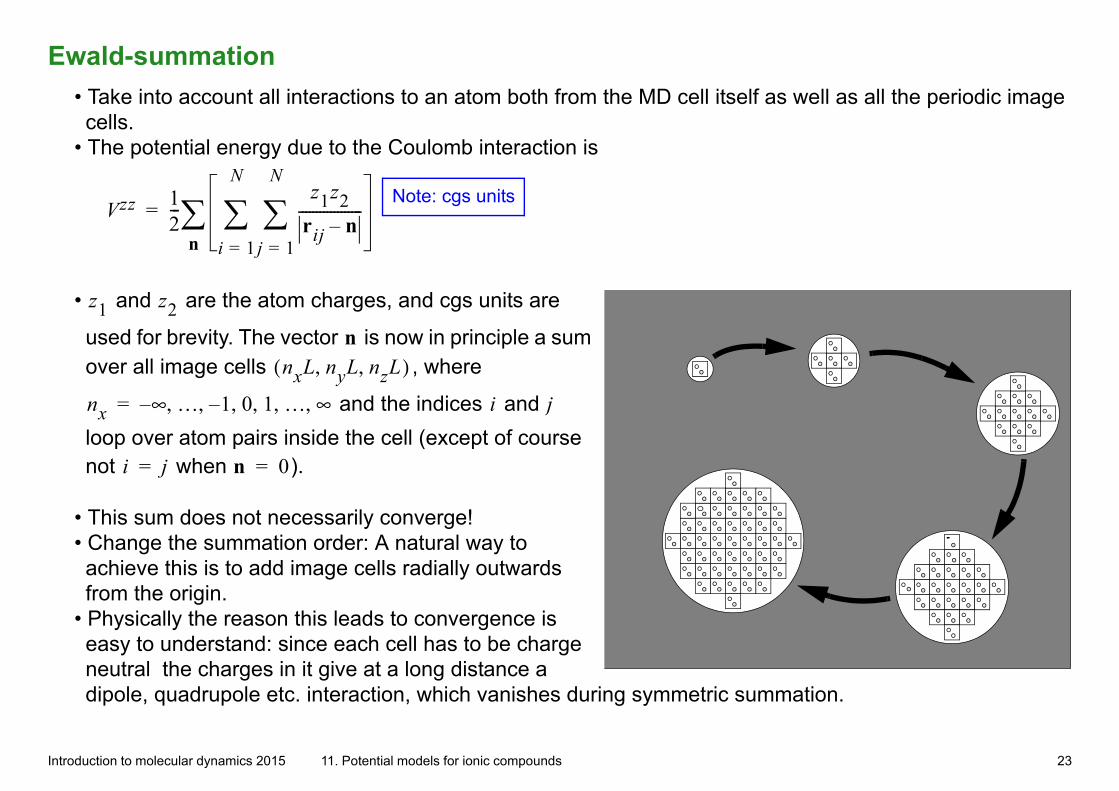
Ewald-summation• Take into account all interactions to an atom both from the MD cell itself as well as all the periodic image cells.

• The potential energy due to the Coulomb interaction is

Vzz 12---

z1z2rij n–------------------

j 1=

N

i 1=

N

n=

Note: cgs units

• z1 and z2 are the atom charges, and cgs units are

used for brevity. The vector n is now in principle a sum over all image cells nxL nyL nzL, ,( ) , where

nx ∞– … 1– 0 1 … ∞, , , , , ,= and the indices i and j

loop over atom pairs inside the cell (except of course not i j= when n 0= ).

• This sum does not necessarily converge! • Change the summation order: A natural way to achieve this is to add image cells radially outwards from the origin.

• Physically the reason this leads to convergence is easy to understand: since each cell has to be charge neutral the charges in it give at a long distance a dipole, quadrupole etc. interaction, which vanishes during symmetric summation.


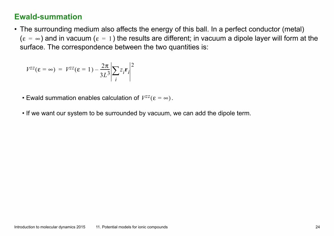
Ewald-summation• The surrounding medium also affects the energy of this ball. In a perfect conductor (metal)

(ε ∞= ) and in vacuum (ε 1= ) the results are different; in vacuum a dipole layer will form at the surface. The correspondence between the two quantities is:

Vzz ε ∞=( ) Vzz ε 1=( ) 2π3L3--------- ziri

i

2–=

• Ewald summation enables calculation of Vzz ε ∞=( ) .

• If we want our system to be surrounded by vacuum, we can add the dipole term.


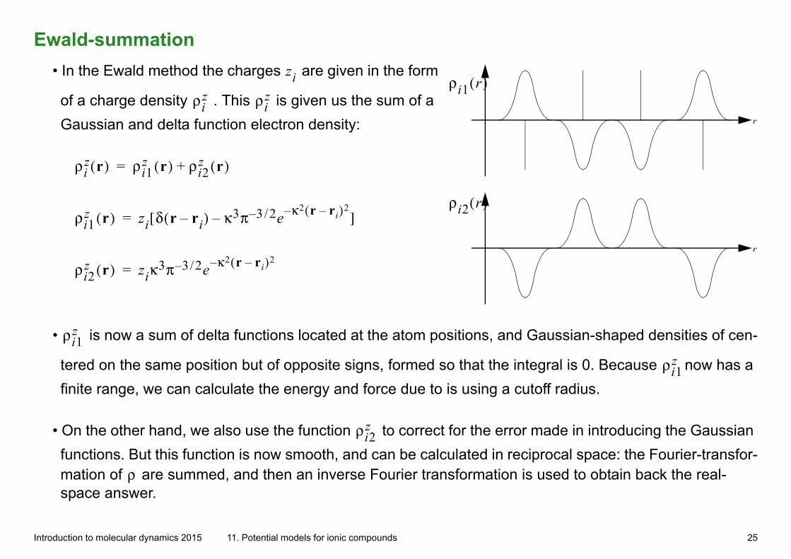
Ewald-summation• In the Ewald method the charges zi are given in the form

of a charge density ρiz . This ρi

z is given us the sum of a

Gaussian and delta function electron density:

r

r

ρi2 r( )

ρi1 r( )

ρiz r( ) ρi1

z r( ) ρi2z r( )+=

ρi1z r( ) zi δ r ri–( ) κ3π 3 2/– e κ2 r ri–( )2––[ ]=

ρi2z r( ) ziκ

3π 3 2/– e κ2 r ri–( )2–=

• ρi1z is now a sum of delta functions located at the atom positions, and Gaussian-shaped densities of cen-

tered on the same position but of opposite signs, formed so that the integral is 0. Because ρi1z now has a

finite range, we can calculate the energy and force due to is using a cutoff radius.

• On the other hand, we also use the function ρi2z to correct for the error made in introducing the Gaussian

functions. But this function is now smooth, and can be calculated in reciprocal space: the Fourier-transfor-mation of ρ are summed, and then an inverse Fourier transformation is used to obtain back the real-space answer.


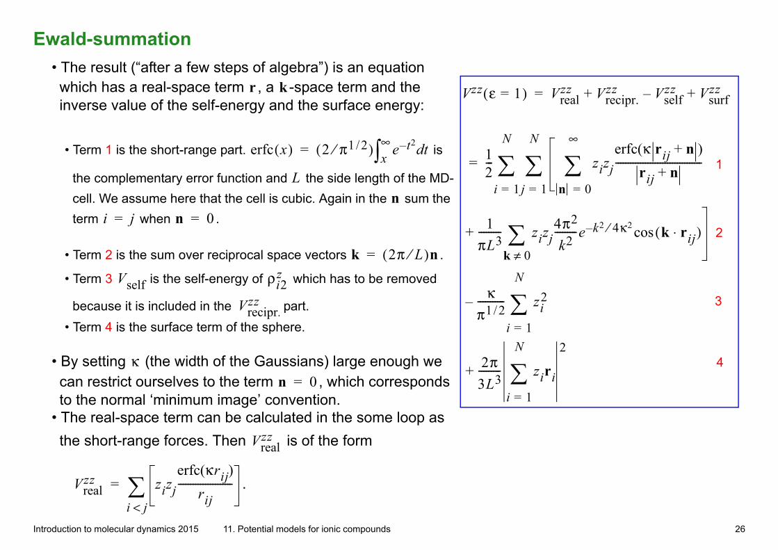
Ewald-summation• The result (“after a few steps of algebra”) is an equation which has a real-space term r , a k -space term and the inverse value of the self-energy and the surface energy:

Vzz ε 1=( ) Vrealzz Vrecipr.

zz Vselfzz Vsurf

zz+–+

12--- zizj

erfc κ rij n+( )rij n+

-----------------------------------

1πL3--------- zizj

4π2

k2---------e k2 4κ2⁄– k rij⋅( )cos

k 0≠+

n 0=

∞

j 1=

N

i 1=

N

κπ1 2/----------- zi

2

i 1=

N

2π3L3--------- ziri

i 1=

N

2

+

–

=

= 1

2

3

4

• Term 1 is the short-range part. erfc x( ) 2 π1 2/⁄( ) e t2– tdx∞= is

the complementary error function and L the side length of the MD-

cell. We assume here that the cell is cubic. Again in the n sum the

term i j= when n 0= .

• Term 2 is the sum over reciprocal space vectors k 2π L⁄( )n= .

• Term 3 Vself is the self-energy of ρi2z which has to be removed

because it is included in the Vrecipr.zz part.

• Term 4 is the surface term of the sphere.

• By setting κ (the width of the Gaussians) large enough we can restrict ourselves to the term n 0= , which corresponds to the normal ‘minimum image’ convention.

• The real-space term can be calculated in the some loop as

the short-range forces. Then Vrealzz is of the form

Vrealzz zizj

erfc κrij( )rij

----------------------i j<= .


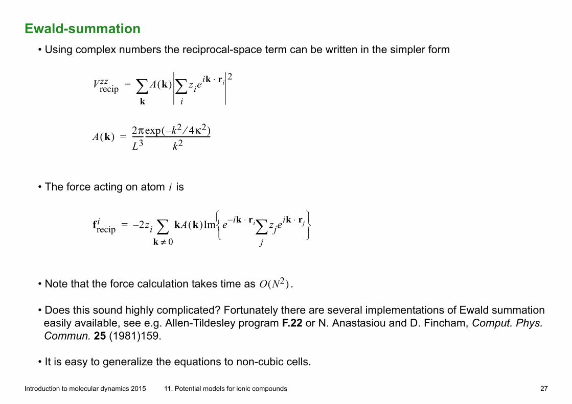
Ewald-summation• Using complex numbers the reciprocal-space term can be written in the simpler form

Vrecipzz A k( ) zie

ik ri⋅

i

2

k=

A k( ) 2πL3------exp k2 4κ2⁄–( )

k2------------------------------------=

• The force acting on atom i is

frecipi 2zi kA k( )Im e ik ri⋅– zje

ik rj⋅

j

k 0≠–=

• Note that the force calculation takes time as O N2( ) .

• Does this sound highly complicated? Fortunately there are several implementations of Ewald summation easily available, see e.g. Allen-Tildesley program F.22 or N. Anastasiou and D. Fincham, Comput. Phys. Commun. 25 (1981)159.

• It is easy to generalize the equations to non-cubic cells.


Ewald-summation• In applying the method one has to choose three parameters:

cutoff radius rc

width of Gaussian charge densities κ upper limit for k summation k max

2 .

• It is best to start by setting rc fairly large, e.g. L 2⁄ . From this a suitable value of κ can be obtained, on the basis of

which a suitable limit for the k -summation can be obtained. Typicallyκ 5 L⁄∼ , in which case the calculation is con-

centrated in k -space. The k -summation would then involve 100-200 vectors.


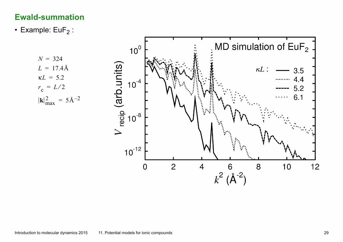
Ewald-summation• Example: EuF2 :

N 324= L 17.4Å= κL 5.2= rc L 2⁄=

k max2 5Å 2–=


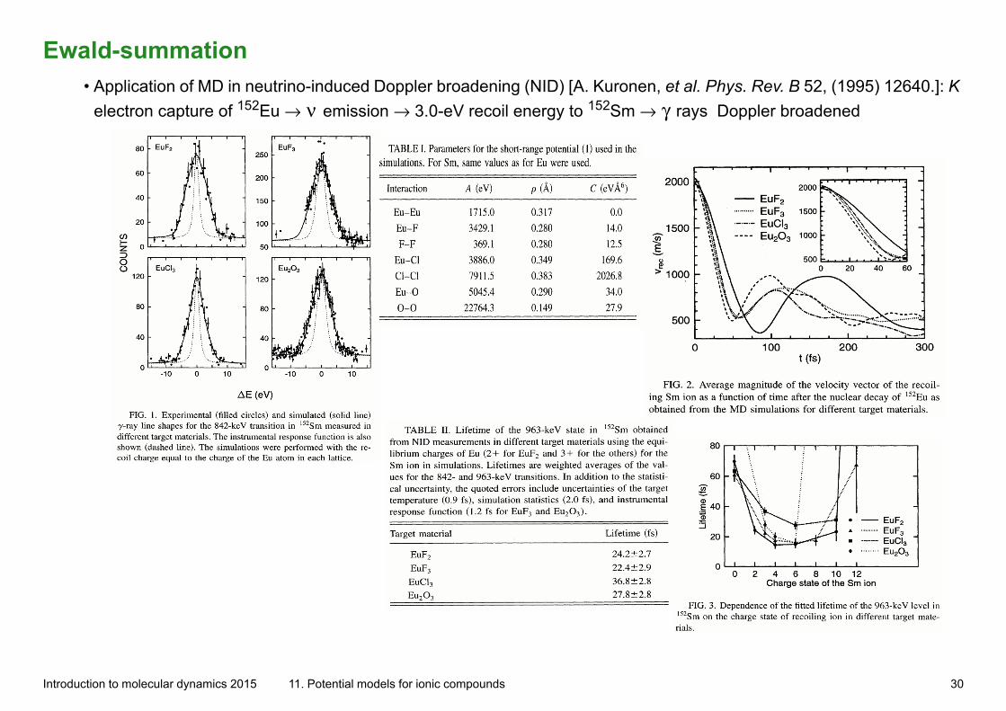
Ewald-summation• Application of MD in neutrino-induced Doppler broadening (NID) [A. Kuronen, et al. Phys. Rev. B 52, (1995) 12640.]: K

electron capture of 152Eu → ν emission → 3.0-eV recoil energy to 152Sm → γ rays Doppler broadened


Ewald-summation• If the periodicity of the Ewald summation causes trouble, one can use the particle-lattice (or par-

ticle-mesh) method:

• The reciprocal space part is calculated by smoothing the ion charges in a regular lattice and solving the potential from

the Poisson equation ∇2φ ρ ε0⁄–= with Fourier methods.

• The advantage is that this scales as O N( ) .

• The disadvantage is that the program gets more complicated

•


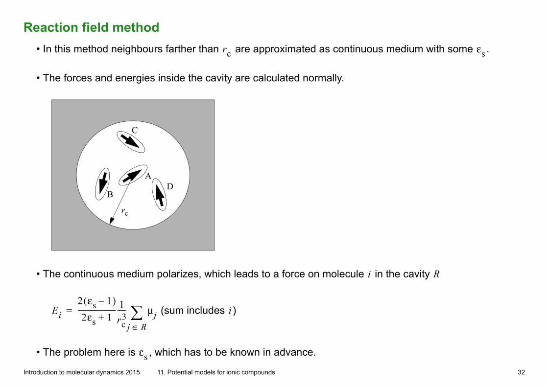
Reaction field method• In this method neighbours farther than rc are approximated as continuous medium with some εs .

• The forces and energies inside the cavity are calculated normally.

A

B

C

D

rc

• The continuous medium polarizes, which leads to a force on molecule i in the cavity R

Ei

2 εs 1–( )2εs 1+

---------------------- 1rc

3----- μj

j R∈= (sum includes i )

• The problem here is εs , which has to be known in advance.


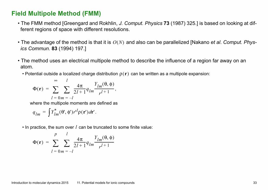
Field Multipole Method (FMM)• The FMM method [Greengard and Rokhlin, J. Comput. Physics 73 (1987) 325.] is based on looking at dif-ferent regions of space with different resolutions.

• The advantage of the method is that it is O N( ) and also can be parallelized [Nakano et al. Comput. Phys-ics Commun. 83 (1994) 197.]

• The method uses an electrical multipole method to describe the influence of a region far away on an atom. • Potential outside a localized charge distribution ρ r( ) can be written as a multipole expansion:

Φ r( ) 4π2l 1+--------------qlm

Ylm θ φ,( )

rl 1+-----------------------

m l–=

l

l 0=

∞

= ,

where the multipole moments are defined as

qlm Ylm* θ' φ',( )r'lρ r'( ) r'd= .

• In practice, the sum over l can be truncated to some finite value:

Φ r( ) 4π2l 1+--------------qlm

Ylm θ φ,( )

rl 1+-----------------------

m l–=

l

l 0=

p

=


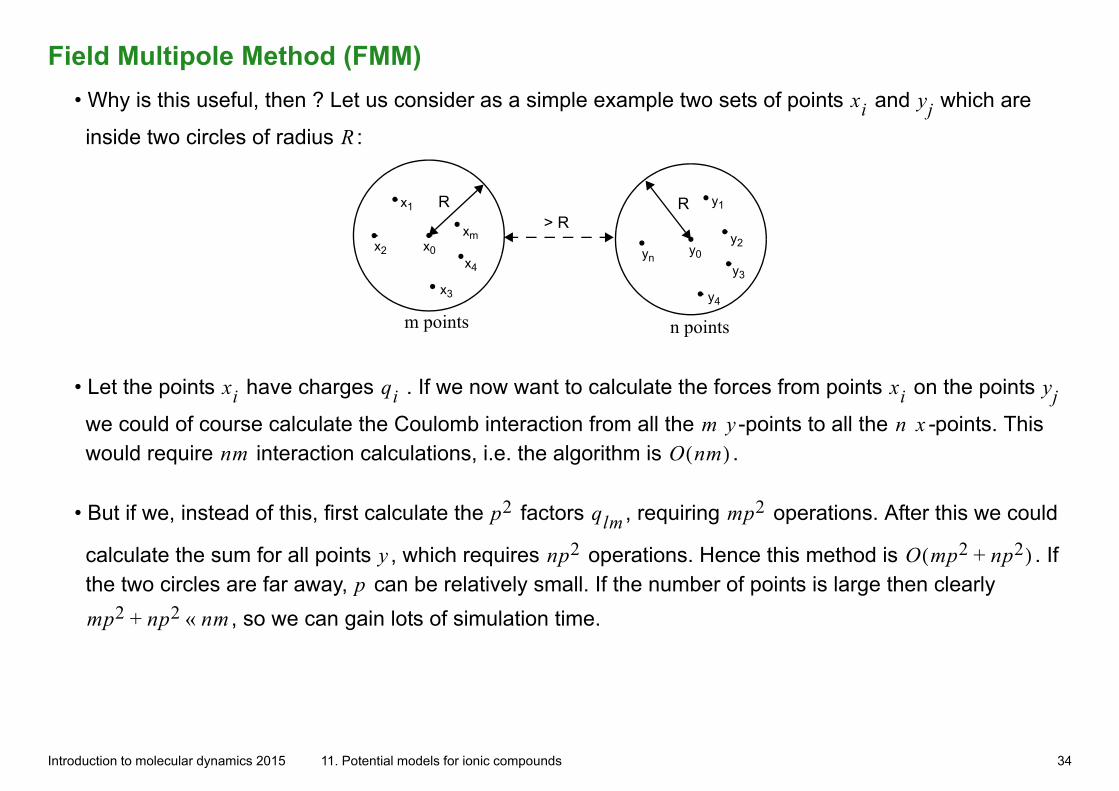
Field Multipole Method (FMM)• Why is this useful, then ? Let us consider as a simple example two sets of points xi and yj which are

inside two circles of radius R :

R R> R

x0 y0

y1

y2

y3

y4

yn

x1

xm

x4

x3

x2

m points n points

• Let the points xi have charges qi . If we now want to calculate the forces from points xi on the points yj

we could of course calculate the Coulomb interaction from all the m y -points to all the n x -points. This would require nm interaction calculations, i.e. the algorithm is O nm( ) .

• But if we, instead of this, first calculate the p2 factors qlm , requiring mp2 operations. After this we could

calculate the sum for all points y , which requires np2 operations. Hence this method is O mp2 np2+( ) . If the two circles are far away, p can be relatively small. If the number of points is large then clearly

mp2 np2+ nm« , so we can gain lots of simulation time.


Field Multipole Method (FMM)

Level 0

Level 1 Level 2 Level 3 Level 4

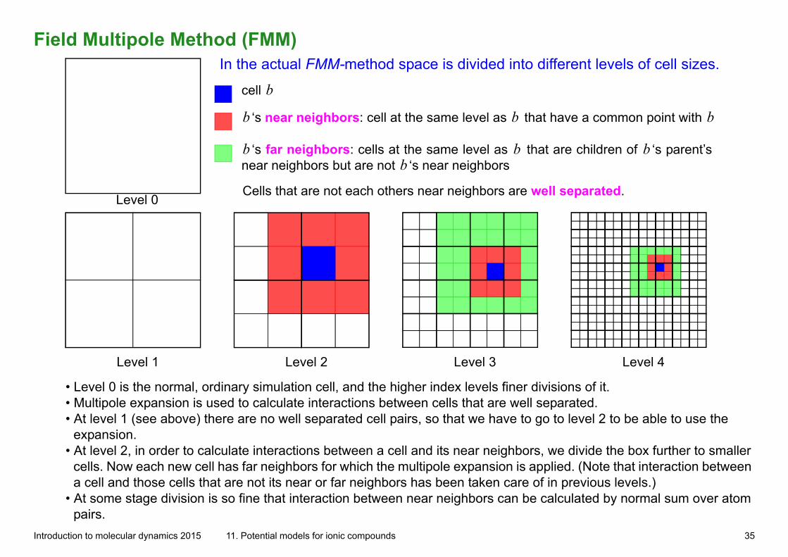
cell b

‘s near neighbors: cell at the same level as that have a common point with b b b

‘s far neighbors: cells at the same level as that are children of ‘s parent’s near neighbors but are not ‘s near neighborsb b b

b

Cells that are not each others near neighbors are well separated.

In the actual FMM-method space is divided into different levels of cell sizes.

• Level 0 is the normal, ordinary simulation cell, and the higher index levels finer divisions of it.• Multipole expansion is used to calculate interactions between cells that are well separated.• At level 1 (see above) there are no well separated cell pairs, so that we have to go to level 2 to be able to use the

expansion. • At level 2, in order to calculate interactions between a cell and its near neighbors, we divide the box further to smaller

cells. Now each new cell has far neighbors for which the multipole expansion is applied. (Note that interaction between a cell and those cells that are not its near or far neighbors has been taken care of in previous levels.)

• At some stage division is so fine that interaction between near neighbors can be calculated by normal sum over atom pairs.


Field Multipole Method (FMM)• This calculation scales as O N Nlog( ) (where N is the number of atoms):

1) at every level the calculation of multipole expansions scales as O p2N( ) 2) number of levels is O Nlog( )

• To obtain the O N( ) behavior multipole expansion is calculated from atom positions only at the smallest scale divisions.• These results can be compined to calculate the expansions in coarser levels by so called translation of a multipole

expansion.

• An accurate algorithm, the equations and boundary condition solutions can be found from the paper of Greengard and Rokhlin.

• In practical calculations numerical noise may become a problem.

• In addition, as in Ewald summation it is also possible to take into account the effect of periodic image cells with the same principle.

• It is also evident that this algorithm can be parallelized well, since for the far cells it is enough to know only the multipole expansion, which is relatively easy to pass around.

• The FMM-model is also very general: in addition to the calculation of atomic interactions it can also be used in plasma dynamics, fluid mechanics and in astronomy!


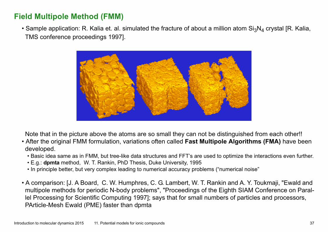
Field Multipole Method (FMM)• Sample application: R. Kalia et. al. simulated the fracture of about a million atom Si3N4 crystal [R. Kalia, TMS conference proceedings 1997].

Note that in the picture above the atoms are so small they can not be distinguished from each other!!

• After the original FMM formulation, variations often called Fast Multipole Algorithms (FMA) have been developed. • Basic idea same as in FMM, but tree-like data structures and FFT’s are used to optimize the interactions even further.• E.g.: dpmta method, W. T. Rankin, PhD Thesis, Duke University, 1995• In principle better, but very complex leading to numerical accuracy problems (“numerical noise”

• A comparison: [J. A Board, C. W. Humphres, C. G. Lambert, W. T. Rankin and A. Y. Toukmaji, "Ewald and multipole methods for periodic N-body problems", "Proceedings of the Eighth SIAM Conference on Paral-lel Processing for Scientific Computing 1997]; says that for small numbers of particles and processors, PArticle-Mesh Ewald (PME) faster than dpmta


T P tt Δt - acclab.helsinki.fiknordlun/moldyn/lecture11.pdf · SR. to describe repulsion ......

Documents

Transcript of T P tt Δt - acclab.helsinki.fiknordlun/moldyn/lecture11.pdf · SR. to describe repulsion ......