Chapter 1

Synchronizability and

Connectivity of

Discrete Complex Systems

Michael Holroyd

College of William and Mary

Williamsburg, Virginia

The synchronization of discrete complex systems is critical in applications such ascommunication and transportation networks, neuron respiratory systems, and othersystems in which either congestion can occur at individual nodes, or system wide syn-chrony is of importance to proper functionality. The first non-trivial eigenvalue of anetwork’s Laplacian matrix, called the algebraic connectivity, provides a quantifiablemeasure of synchronizability in a network. We study the general relationship betweennetwork topology, clustering coefficient distributions, and synchronizability, as well asthe effects of degree preserving rewiring on network synchronizability. In addition,we compare the synchronizability of different network topologies, including Poissonrandom graphs, geometric networks, preferential attachment networks, and scale-richnetworks. We also explore uses of the algebraic connectivity in the design and man-agement of complex networks where synchronization is desired (respiration networks),or detrimental to network performance (router networks).

1.1 Background

In the study of discrete complex systems, it is often important to understand thelikelihood of synchronization on a given network. For example, synchronizationin air transportation networks results in delays and congestion at airports.

Consider the network of nodes (airports, routers, neurons) and edges connect-

2 Synchronizability and Connectivity of Discrete Complex Systems

ing them (flights, ethernet, axons) that models such a complex system. Denotethe state of node i at time t by xi(t). How do the states of all nodes changeover time? Clearly if nodes do not take any note of their neighbors there is nochance for synchronization.

As in [1], we assume that all nodes are identical and conform to the followinggeneric discrete time equation to determine their next state:

xi(t + 1) = f(xi(t)) + κ

1

ki

∑

j|i↔j

f(xj(t)) − f(xi(t))

(1.1)

where i ↔ j denotes an edge between i and j [1]. κ is called the coupling

strength and is a scalar describing the extent to which neighbors effect the stateof a node. f(x) is any differentiable function that describes the behavior of anode in the absence of outside influence: notice that if κ = 0, the equation issimply xi(t + 1) = f(xi(t)).

An initial condition (x1(0), · · · , xn(0)) synchronizes if for all i, j

limt→∞

|xi(t) − xj(t)| = 0 (1.2)

and we say that the entire network synchronizes if x1 = · · · = xn is anattracting set.

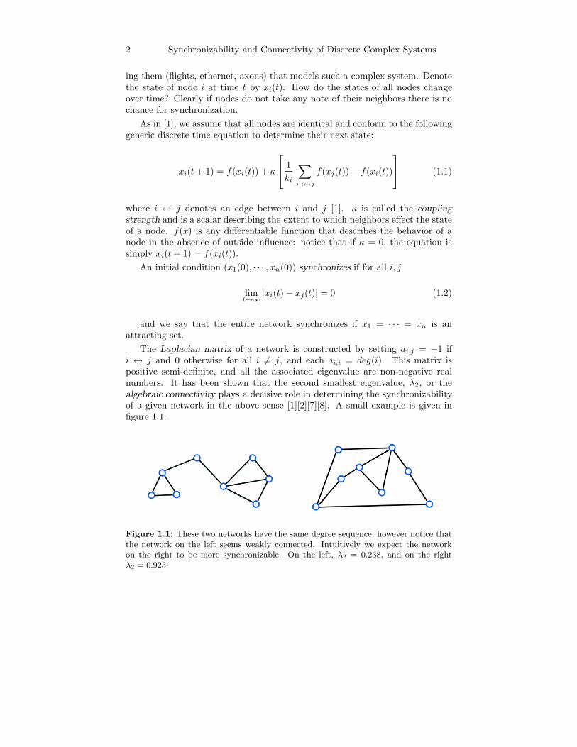
The Laplacian matrix of a network is constructed by setting ai,j = −1 ifi ↔ j and 0 otherwise for all i 6= j, and each ai,i = deg(i). This matrix ispositive semi-definite, and all the associated eigenvalue are non-negative realnumbers. It has been shown that the second smallest eigenvalue, λ2, or thealgebraic connectivity plays a decisive role in determining the synchronizabilityof a given network in the above sense [1][2][7][8]. A small example is given infigure 1.1.

Figure 1.1: These two networks have the same degree sequence, however notice thatthe network on the left seems weakly connected. Intuitively we expect the networkon the right to be more synchronizable. On the left, λ2 = 0.238, and on the rightλ2 = 0.925.

Synchronizability and Connectivity of Discrete Complex Systems 3

1.2 λ2 of Erdos-Renyi random graphs

In the Erdos-Renyi, or Gn,p, construction first defined by Paul Erdos and AlfredRenyi in [5], we take n nodes and between each pair of nodes create an edgewith probability p. This type of network is often referred to as a Poisson ran-dom graph, since for large n the degree distribution tends toward a Poissondistribution [4].

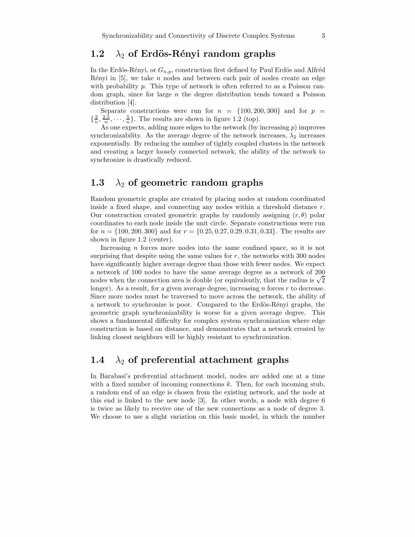
Separate constructions were run for n = {100, 200, 300} and for p ={ 2

n, 2.5

n, · · · , 5

n}. The results are shown in figure 1.2 (top).

As one expects, adding more edges to the network (by increasing p) improvessynchronizability. As the average degree of the network increases, λ2 increasesexponentially. By reducing the number of tightly coupled clusters in the networkand creating a larger loosely connected network, the ability of the network tosynchronize is drastically reduced.

1.3 λ2 of geometric random graphs

Random geometric graphs are created by placing nodes at random coordinatedinside a fixed shape, and connecting any nodes within a threshold distance r.Our construction created geometric graphs by randomly assigning (r, θ) polarcoordinates to each node inside the unit circle. Separate constructions were runfor n = {100, 200, 300} and for r = {0.25, 0.27, 0.29, 0.31, 0.33}. The results areshown in figure 1.2 (center).

Increasing n forces more nodes into the same confined space, so it is notsurprising that despite using the same values for r, the networks with 300 nodeshave significantly higher average degree than those with fewer nodes. We expecta network of 100 nodes to have the same average degree as a network of 200nodes when the connection area is double (or equivalently, that the radius is

√2

longer). As a result, for a given average degree, increasing n forces r to decrease.Since more nodes must be traversed to move across the network, the ability ofa network to synchronize is poor. Compared to the Erdos-Renyi graphs, thegeometric graph synchronizability is worse for a given average degree. Thisshows a fundamental difficulty for complex system synchronization where edgeconstruction is based on distance, and demonstrates that a network created bylinking closest neighbors will be highly resistant to synchronization.

1.4 λ2 of preferential attachment graphs

In Barabasi’s preferential attachment model, nodes are added one at a timewith a fixed number of incoming connections k. Then, for each incoming stub,a random end of an edge is chosen from the existing network, and the node atthis end is linked to the new node [3]. In other words, a node with degree 6is twice as likely to receive one of the new connections as a node of degree 3.We choose to use a slight variation on this basic model, in which the number

4 Synchronizability and Connectivity of Discrete Complex Systems

0

0.1

0.2

0.3

0.4

0.5

0.6

0.7

2 2.5 3 3.5 4 4.5 5 5.5

λ2 -

Alg

ebra

ic c

onn

ecti

vity

Average degree

Erdös-Rényi random graph

N = 100N = 200N = 300

0

0.5

1

1.5

2

2.5

5 10 15 20 25 30 35

λ2 (A

lgeb

raic

con

nec

tivi

ty)

Average degree

Geometric random graph on the unit square

N = 100N = 200N = 300

0

0.1

0.2

0.3

0.4

0.5

0.6

0.7

0.8

0.9

2 3 4 5 6 7 8

λ2 (A

lgeb

raic

con

nec

tivi

ty)

Average degree

Preferential Attachment

N = 100N = 200N = 300

Figure 1.2: Plots depicting the relationship between average degree and λ2 for ran-domly generated Erdos-Renyi graphs (top), geometric graphs (center), and preferentialattachment graphs (bottom). N is the number of nodes in the network.

Synchronizability and Connectivity of Discrete Complex Systems 5

of incoming connections for a new node is uniformly random from 1 to k. Thisresults in a wider variety of networks with different average degrees centeredaround k + 1. Separate constructions were run for k = {2, 3, 4, 5, 6} and forn = {100, 200, 300}. The results are shown in figure 1.2 (bottom).

We see an unexpected phenomena in the data, resulting in some clusteringof datapoints along the y axis, especially just beneath λ2 = 0.4. By observingspecific networks on opposite sides of this divide, it became clear that this strangebehavior was due to the “winner takes all” scenario, in which an early node in thenetwork construction gains an unusually large degree very quickly. New nodesprefer to connect with high degree nodes, so a single node of very high degreecauses most new nodes to connect with it. A network which relies on a singlehighly connected hub is less synchronizable than a network centered around acore of several nodes.

1.5 Neuron rhythmogensis

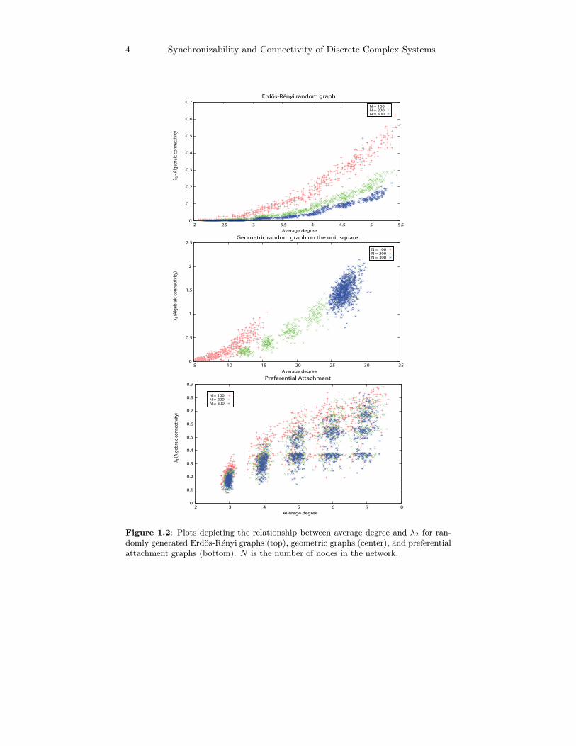
In mammals, a small group of neurons in the brainstem called the pre-Botzingercomplex is responsible for generating a regular rhythmic output to motor cellsthat initiate a breath. Disconnected, these neurons are unable to provide enoughoutput to activate the motor neurons, but their interconnected network structureallows them to synchronize without any external influence and produce regularbursts. An example of a typical neuron’s output is in figure 1.3.

Vm

40

mV

Figure 1.3: Example output from an individual neuron in the PreBotzinger complex.This function corresponds to f(x) in equation 1.1.

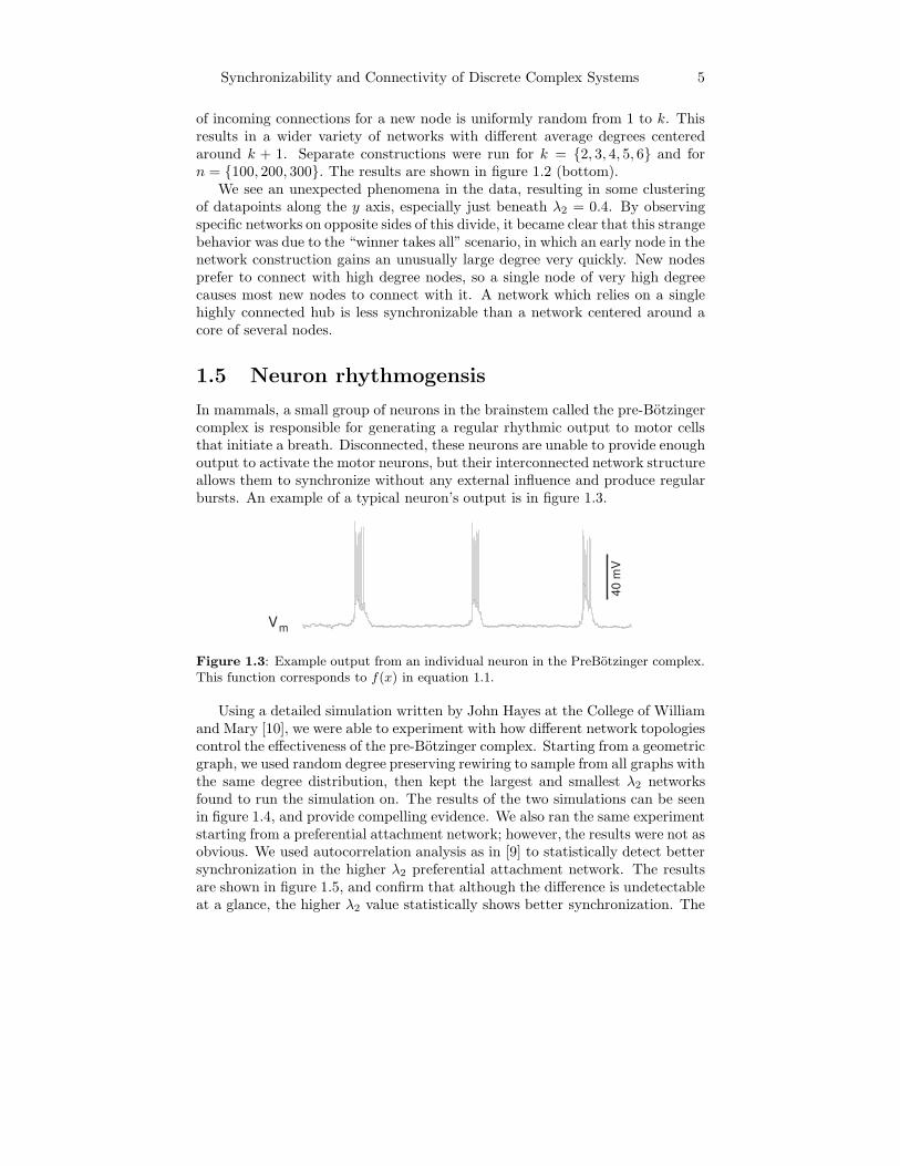
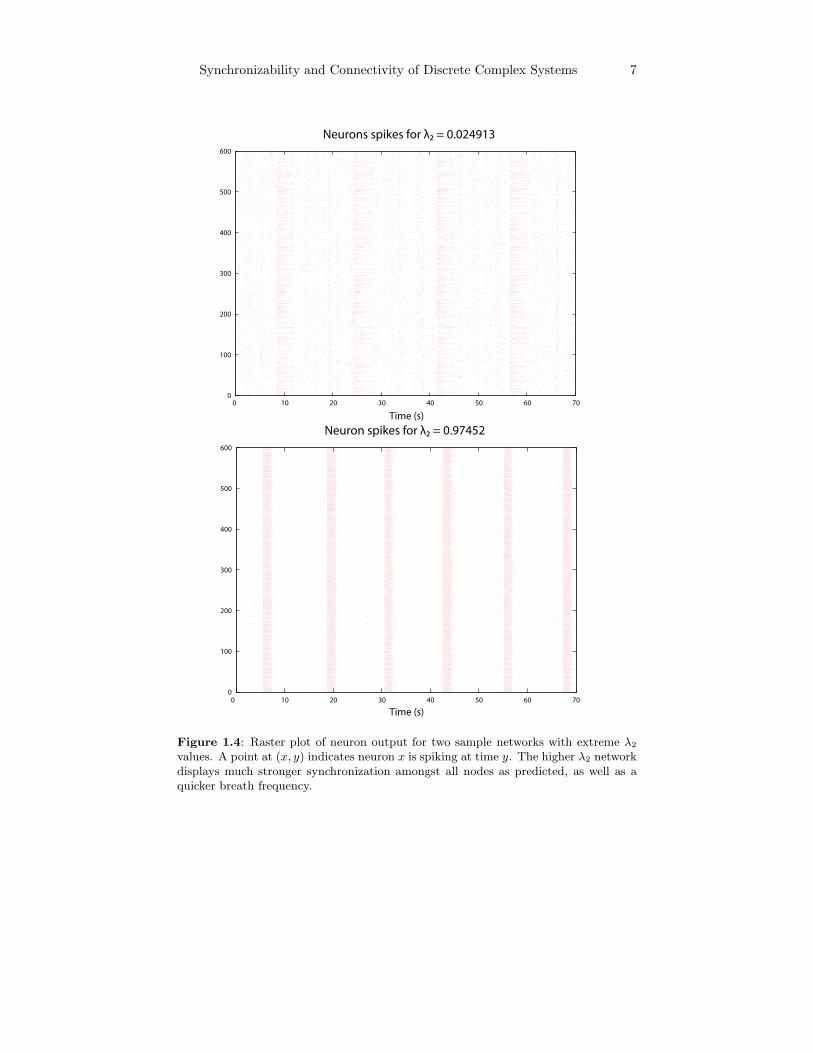
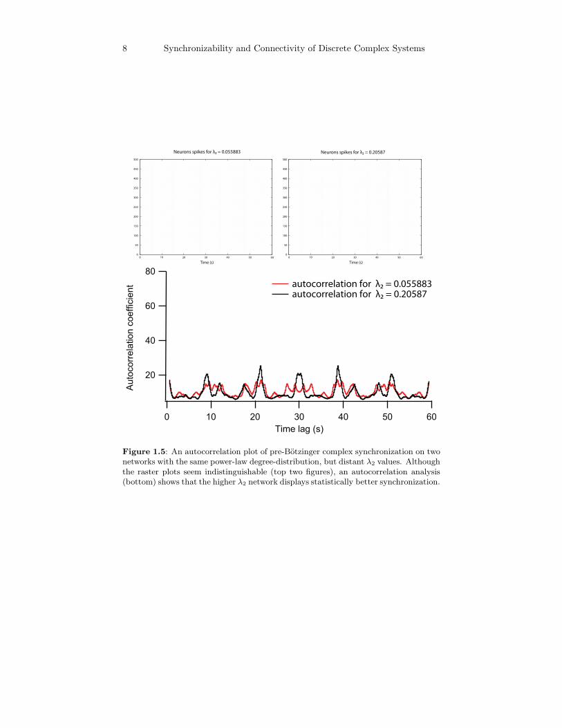
Using a detailed simulation written by John Hayes at the College of Williamand Mary [10], we were able to experiment with how different network topologiescontrol the effectiveness of the pre-Botzinger complex. Starting from a geometricgraph, we used random degree preserving rewiring to sample from all graphs withthe same degree distribution, then kept the largest and smallest λ2 networksfound to run the simulation on. The results of the two simulations can be seenin figure 1.4, and provide compelling evidence. We also ran the same experimentstarting from a preferential attachment network; however, the results were not asobvious. We used autocorrelation analysis as in [9] to statistically detect bettersynchronization in the higher λ2 preferential attachment network. The resultsare shown in figure 1.5, and confirm that although the difference is undetectableat a glance, the higher λ2 value statistically shows better synchronization. The

6 Synchronizability and Connectivity of Discrete Complex Systems

difference in autocorrelation is largest during the refractory (non-spiking) period,indicating that the two networks have similar behavior during the spikes, butnot between spikes. For more details, see the original paper at [6].

Acknowledgements

This research was supported in part by a Howard Hughes Medical Institutegrant through the Undergraduate Biological Sciences Education Program to theCollege of William & Mary.

Bibliography

[1] Atay, Fatihcan M., Tuerker Biyikoglu, and Juergen Jost, “Synchro-nization of networks with prescribed degree distributions” (May 29 2004).

[2] Atay, Fatihcan M., Jurgen Jost, and Andreas Wende, “Delays, con-nection topology, and synchronization of coupled chaotic maps” (Apr. 112003).

[3] Barabasi, Albert-Laszlo, and Reka Albert, “Emergence of scaling inrandom networks”, Science 286, 5439 (Oct. 1999), 509–512.

[4] Callaway, D. S., M. E. J. Newman, S. H. Strogatz, and D. J. Watts,“Network robustness and fragility: Percolation on random graphs” (Oct. 192000), Comment: 4 pages, 2 figures.

[5] Erdos, Paul, and A. Renyi, “On random graphs I”, Publicationes Math-

ematicae 6 (1959), 290–297.

[6] Holroyd, Michael, “Synchronizability and connectivity of discrete com-plex systems” (Apr. 2006).

[7] Hong, H., M. Y. Choi, and Beom Jun Kim, “Synchronization on small-world networks” (Oct. 17 2001).

[8] Jost, J., and M. P. Joy, “Spectral properties and synchronization incoupled map lattices” (Oct. 19 2001), To appear in PRE.

[9] Kosmidis, E. K., O. Pierrefiche, and J. F. Vibert, “Respiratory-like rhythmic activity can be produced by an excitatory network of non-pacemaker neuron models”, Journal of Neurophysiology 92 (2004), 686–699.

[10] Negro, Christopher Del, John Hayes, C. Morgadi-Valle, D. D.Mackay, R. W. Pace, E. A. Crowder, and J. L. Feldman, “Sodiumand calcium current-mediated pacemaker neurons and respiratory rhythmgeneration.”, J. Neurosci. 25 (Jan. 2005), 446–53.

Synchronizability and Connectivity of Discrete Complex Systems 7

0

100

200

300

400

500

600

0 10 20 30 40 50 60 70

Time (s)

Neurons spikes for λ2 = 0.024913

0

100

200

300

400

500

600

0 10 20 30 40 50 60 70

Time (s)

Neuron spikes for λ2 = 0.97452

Figure 1.4: Raster plot of neuron output for two sample networks with extreme λ2

values. A point at (x, y) indicates neuron x is spiking at time y. The higher λ2 networkdisplays much stronger synchronization amongst all nodes as predicted, as well as aquicker breath frequency.

8 Synchronizability and Connectivity of Discrete Complex Systems

0

50

100

150

200

250

300

350

400

450

500

0 10 20 30 40 50 60

Time (s)

Neurons spikes for λ2 = 0.055883

0

50

100

150

200

250

300

350

400

450

500

0 10 20 30 40 50 60

Time (s)

Neurons spikes for λ2 = 0.20587

80

60

40

20

Auto

co

rrela

tion

coeffic

ien

t

6050403020100

Time lag (s)

autocorrelation for λ2 = 0.055883 autocorrelation for λ2 = 0.20587

Figure 1.5: An autocorrelation plot of pre-Botzinger complex synchronization on twonetworks with the same power-law degree-distribution, but distant λ2 values. Althoughthe raster plots seem indistinguishable (top two figures), an autocorrelation analysis(bottom) shows that the higher λ2 network displays statistically better synchronization.