Symmetry Methods forDifferential Equationsand Conservation Laws

Peter J. Olver

University of Minnesota

http://www.math.umn.edu/∼ olver

Santiago, November, 2010

Symmetry Groups of

Differential Equations

System of differential equations

∆(x, u(n)) = 0

G — Lie group acting on the space of independentand dependent variables:

(x, u) = g · (x, u) = (Ξ(x, u), Φ(x, u))

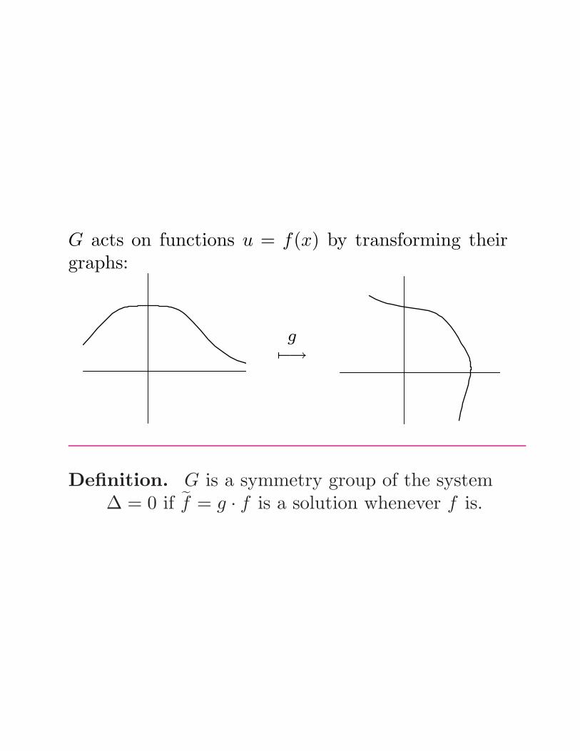
G acts on functions u = f(x) by transforming theirgraphs:

g7−→

Definition. G is a symmetry group of the system∆ = 0 if f = g · f is a solution whenever f is.

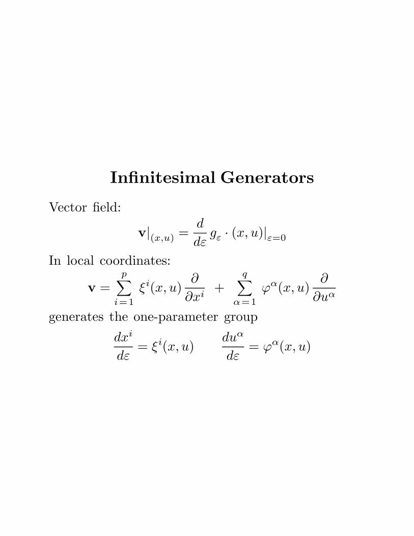
Infinitesimal Generators

Vector field:

v|(x,u) =d

dεgε · (x, u)|ε=0

In local coordinates:

v =p∑

i=1

ξi(x, u)∂

∂xi+

q∑

α=1

ϕα(x, u)∂

∂uα

generates the one-parameter group

dxi

dε= ξi(x, u)

duα

dε= ϕα(x, u)

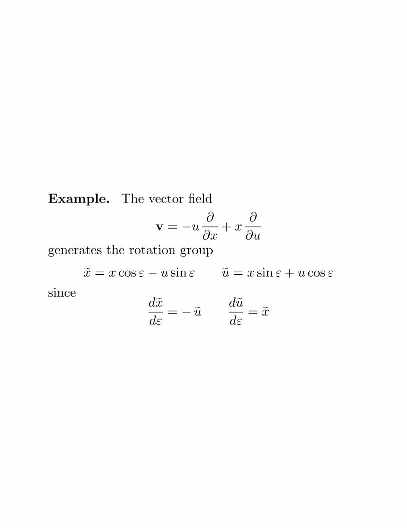
Example. The vector field

v = −u∂

∂x+ x

∂

∂ugenerates the rotation group

x = x cos ε − u sin ε u = x sin ε + u cos ε

sincedx

dε= − u

du

dε= x

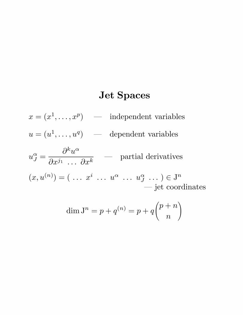
Jet Spaces

x = (x1, . . . , xp) — independent variables

u = (u1, . . . , uq) — dependent variables

uαJ =

∂kuα

∂xj1 . . . ∂xk— partial derivatives

(x, u(n)) = ( . . . xi . . . uα . . . uαJ . . . ) ∈ Jn

— jet coordinates

dimJn = p + q(n) = p + q

(p + n

n

)

Prolongation to Jet Space

Since G acts on functions, it acts on their derivatives,leading to the prolonged group action on the jet space:

(x, u(n)) = pr(n) g · (x, u(n))

=⇒ formulas provided by implicit differentiation

Prolonged vector field or infinitesimal generator:

pr v = v +∑

α,J

ϕαJ(x, u(n))

∂

∂uαJ

The coefficients of the prolonged vector field are givenby the explicit prolongation formula:

ϕαJ = DJ Qα +

p∑

i=1

ξi uαJ,i

Q = (Q1, . . . , Qq) — characteristic of v

Qα(x, u(1)) = ϕα −p∑

i=1

ξi ∂uα

∂xi

⋆ Invariant functions are solutions to

Q(x, u(1)) = 0.

Symmetry Criterion

Theorem. (Lie) A connected group of transforma-tions G is a symmetry group of a nondegeneratesystem of differential equations ∆ = 0 if and only if

pr v(∆) = 0 (∗)whenever u is a solution to ∆ = 0 for every infinitesi-mal generator v of G.

(*) are the determining equations of the symmetrygroup to ∆ = 0. For nondegenerate systems, thisis equivalent to

pr v(∆) = A · ∆ =∑

νAν∆ν

Nondegeneracy Conditions

Maximal Rank:

rank

(· · · ∂∆ν

∂xi· · · ∂∆ν

∂uαJ

· · ·)

= max

Local Solvability: Any each point (x0, u(n)0 ) such that

∆(x0, u(n)0 ) = 0

there exists a solution u = f(x) with

u(n)0 = pr(n) f(x0)

Nondegenerate = maximal rank + locally solvable

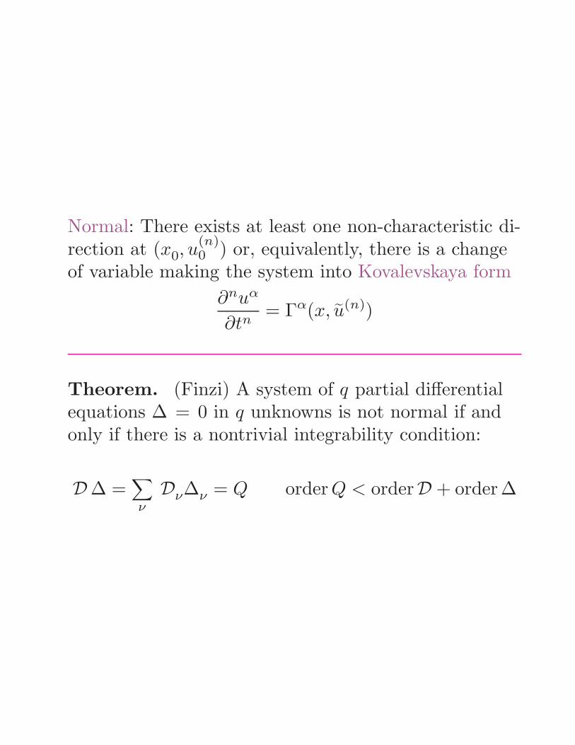
Normal: There exists at least one non-characteristic di-rection at (x0, u

(n)0 ) or, equivalently, there is a change

of variable making the system into Kovalevskaya form

∂nuα

∂tn= Γα(x, u(n))

Theorem. (Finzi) A system of q partial differentialequations ∆ = 0 in q unknowns is not normal if andonly if there is a nontrivial integrability condition:

D∆ =∑

νDν∆ν = Q order Q < orderD + order ∆

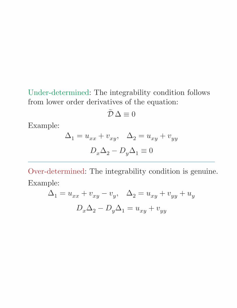
Under-determined: The integrability condition followsfrom lower order derivatives of the equation:

D∆ ≡ 0

Example:

∆1 = uxx + vxy, ∆2 = uxy + vyy

Dx∆2 − Dy∆1 ≡ 0

Over-determined: The integrability condition is genuine.

Example:

∆1 = uxx + vxy − vy, ∆2 = uxy + vyy + uy

Dx∆2 − Dy∆1 = uxy + vyy

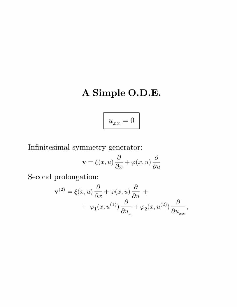
A Simple O.D.E.

uxx = 0

Infinitesimal symmetry generator:

v = ξ(x, u)∂

∂x+ ϕ(x, u)

∂

∂u

Second prolongation:

v(2) = ξ(x, u)∂

∂x+ ϕ(x, u)

∂

∂u+

+ ϕ1(x, u(1))∂

∂ux

+ ϕ2(x, u(2))∂

∂uxx

,

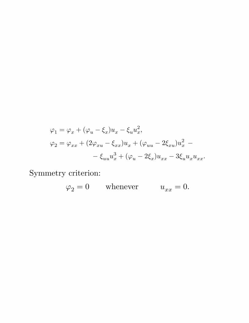
ϕ1 = ϕx + (ϕu − ξx)ux − ξuu2x,

ϕ2 = ϕxx + (2ϕxu − ξxx)ux + (ϕuu − 2ξxu)u2x −

− ξuuu3x + (ϕu − 2ξx)uxx − 3ξuuxuxx.

Symmetry criterion:

ϕ2 = 0 whenever uxx = 0.

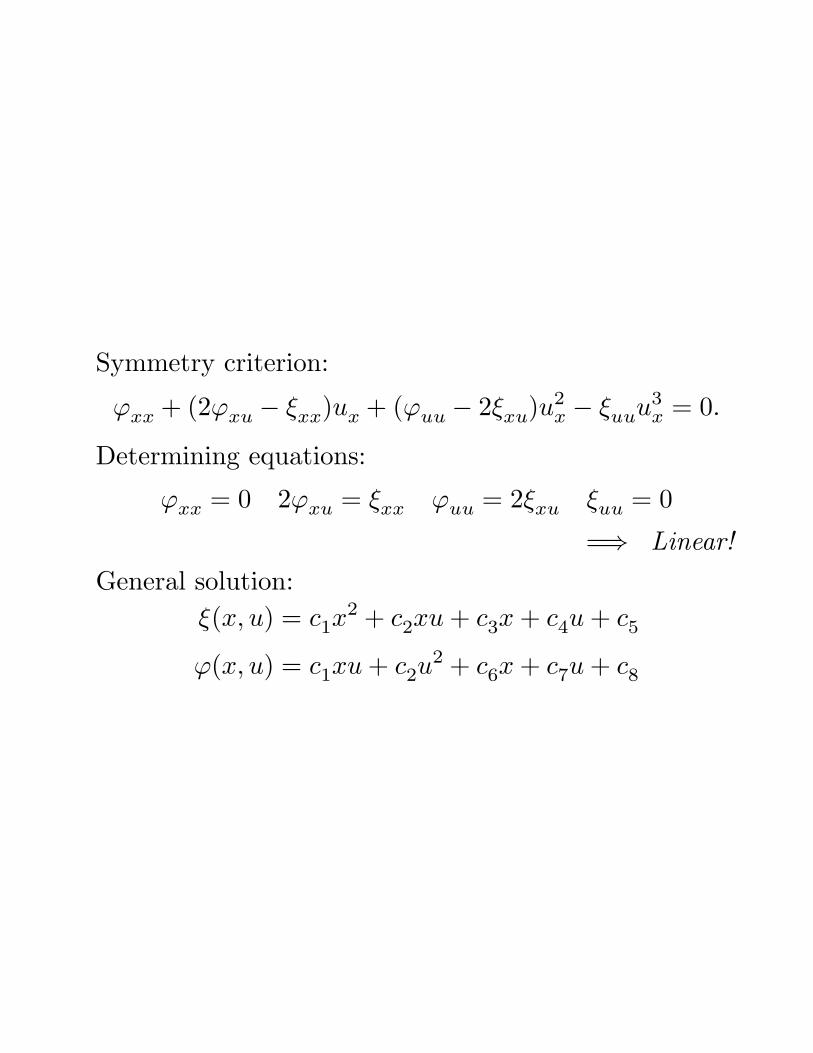
Symmetry criterion:

ϕxx + (2ϕxu − ξxx)ux + (ϕuu − 2ξxu)u2x − ξuuu3

x = 0.

Determining equations:

ϕxx = 0 2ϕxu = ξxx ϕuu = 2ξxu ξuu = 0

=⇒ Linear!

General solution:

ξ(x, u) = c1x2 + c2xu + c3x + c4u + c5

ϕ(x, u) = c1xu + c2u2 + c6x + c7u + c8

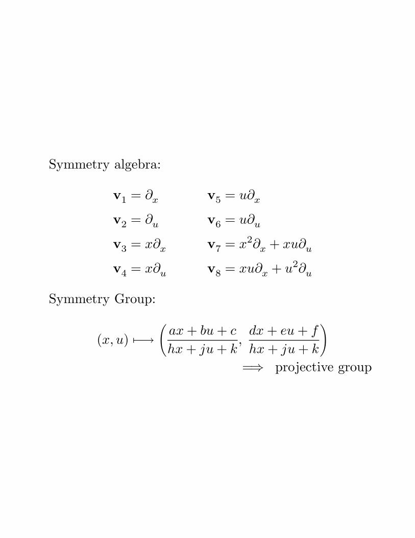
Symmetry algebra:

v1 = ∂x

v2 = ∂u

v3 = x∂x

v4 = x∂u

v5 = u∂x

v6 = u∂u

v7 = x2∂x + xu∂u

v8 = xu∂x + u2∂u

Symmetry Group:

(x, u) 7−→(

ax + bu + c

hx + ju + k,

dx + eu + f

hx + ju + k

)

=⇒ projective group

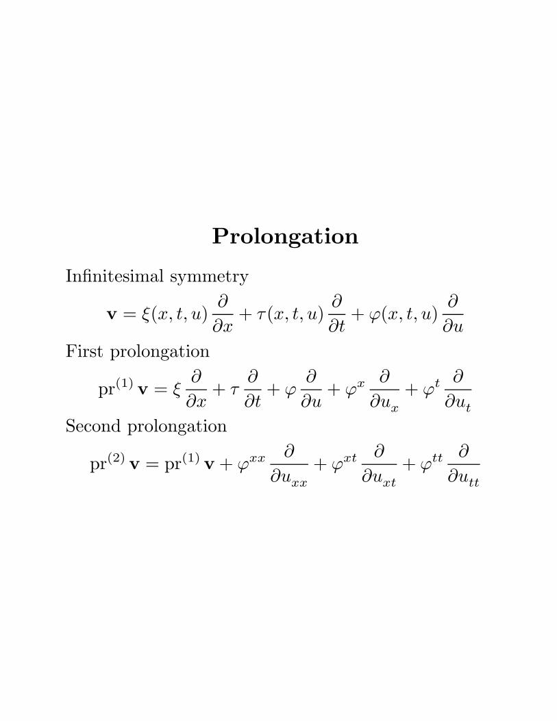
Prolongation

Infinitesimal symmetry

v = ξ(x, t, u)∂

∂x+ τ (x, t, u)

∂

∂t+ ϕ(x, t, u)

∂

∂u

First prolongation

pr(1) v = ξ∂

∂x+ τ

∂

∂t+ ϕ

∂

∂u+ ϕx ∂

∂ux

+ ϕt ∂

∂ut

Second prolongation

pr(2) v = pr(1) v + ϕxx ∂

∂uxx

+ ϕxt ∂

∂uxt

+ ϕtt ∂

∂utt

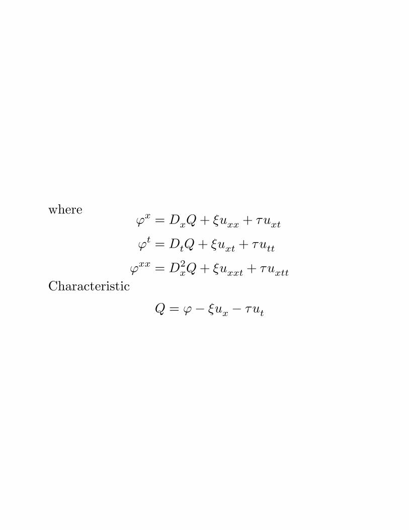
whereϕx = DxQ + ξuxx + τuxt

ϕt = DtQ + ξuxt + τutt

ϕxx = D2xQ + ξuxxt + τuxtt

Characteristic

Q = ϕ − ξux − τut

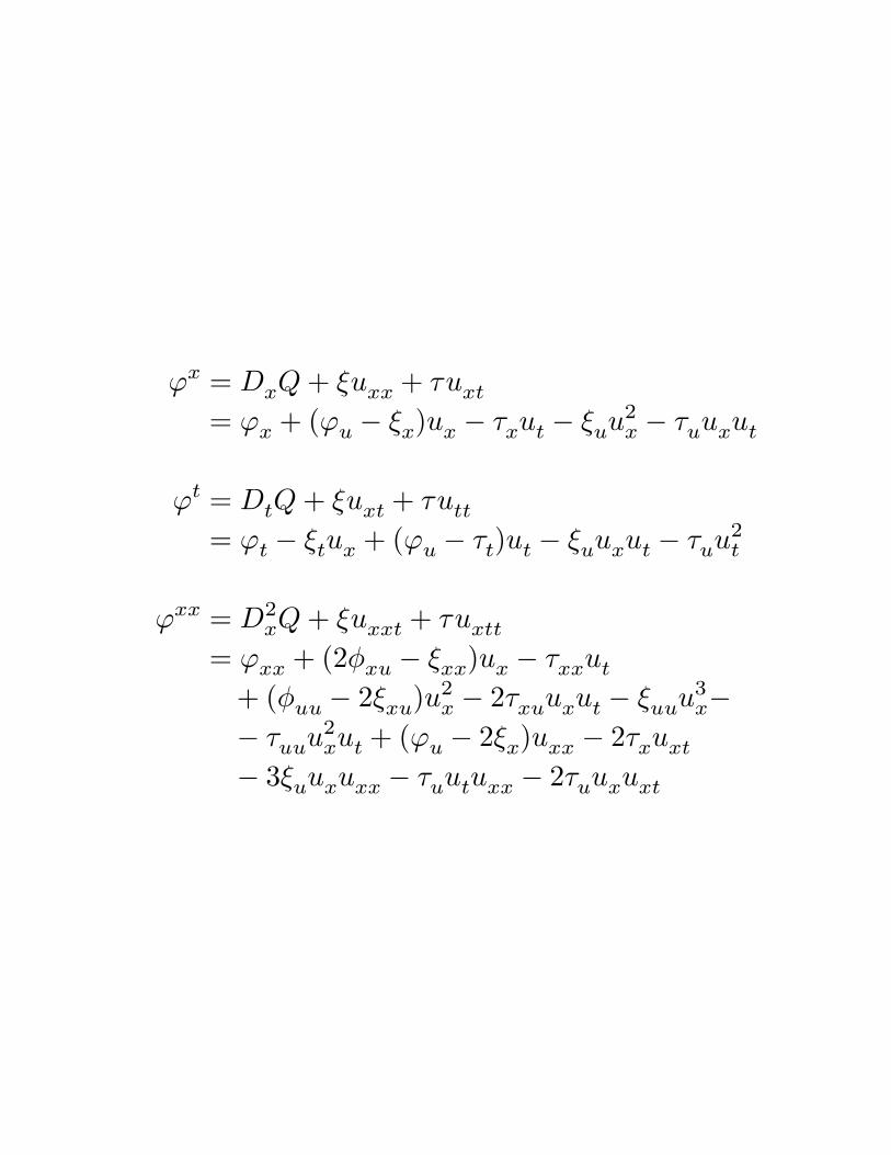
ϕx = DxQ + ξuxx + τuxt

= ϕx + (ϕu − ξx)ux − τxut − ξuu2x − τuuxut

ϕt = DtQ + ξuxt + τutt

= ϕt − ξtux + (ϕu − τt)ut − ξuuxut − τuu2t

ϕxx = D2xQ + ξuxxt + τuxtt

= ϕxx + (2φxu − ξxx)ux − τxxut

+ (φuu − 2ξxu)u2x − 2τxuuxut − ξuuu3

x−− τuuu2

xut + (ϕu − 2ξx)uxx − 2τxuxt

− 3ξuuxuxx − τuutuxx − 2τuuxuxt

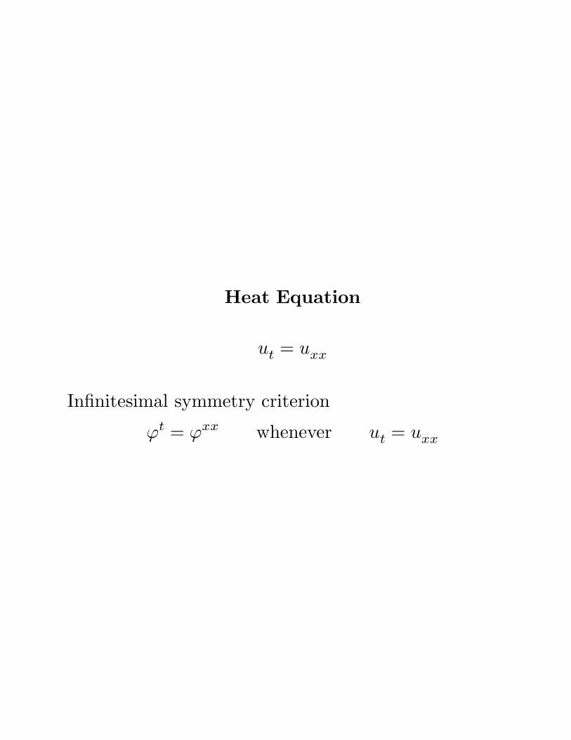
Heat Equation

ut = uxx

Infinitesimal symmetry criterion

ϕt = ϕxx whenever ut = uxx

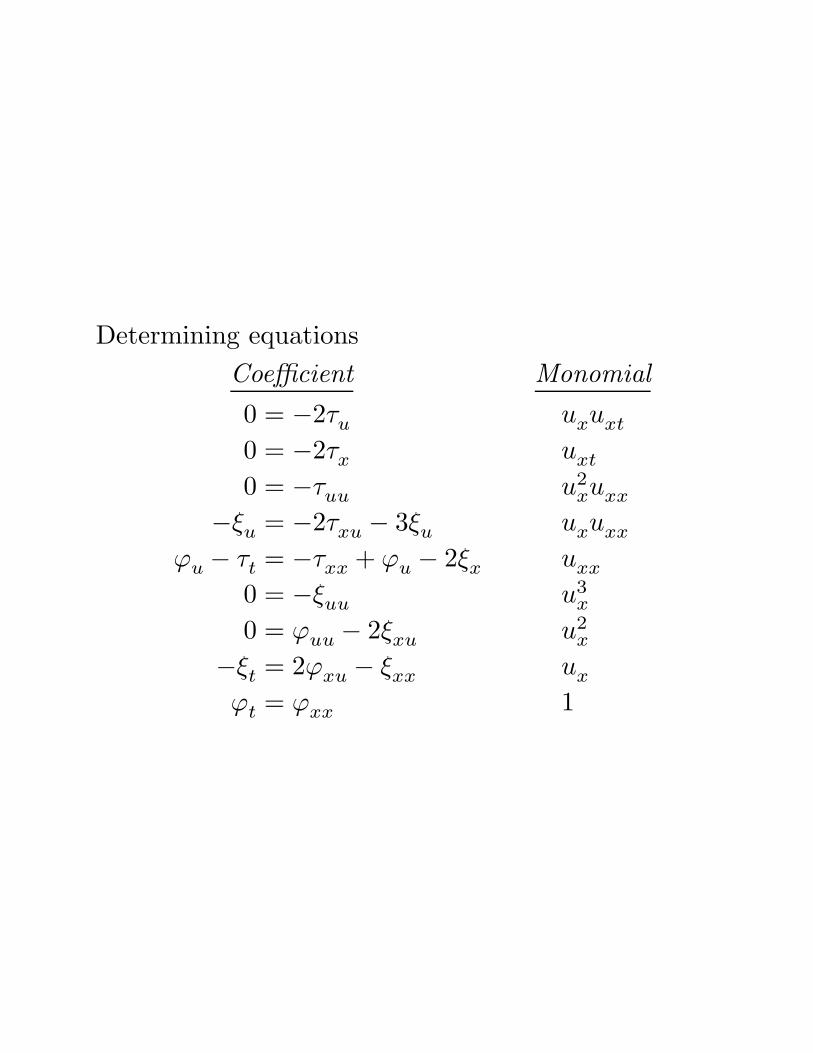
Determining equations

Coefficient Monomial

0 = −2τu uxuxt

0 = −2τx uxt

0 = −τuu u2xuxx

−ξu = −2τxu − 3ξu uxuxx

ϕu − τt = −τxx + ϕu − 2ξx uxx

0 = −ξuu u3x

0 = ϕuu − 2ξxu u2x

−ξt = 2ϕxu − ξxx ux

ϕt = ϕxx 1

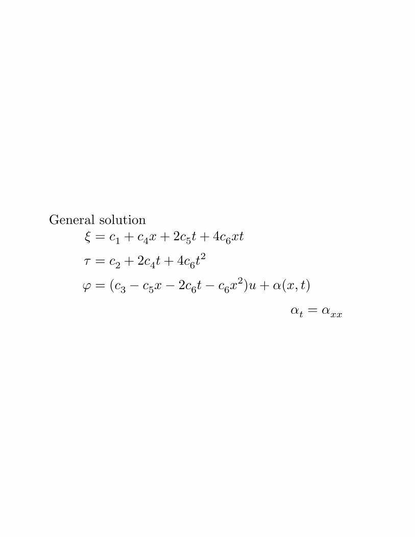
General solutionξ = c1 + c4x + 2c5t + 4c6xt

τ = c2 + 2c4t + 4c6t2

ϕ = (c3 − c5x − 2c6t − c6x2)u + α(x, t)

αt = αxx

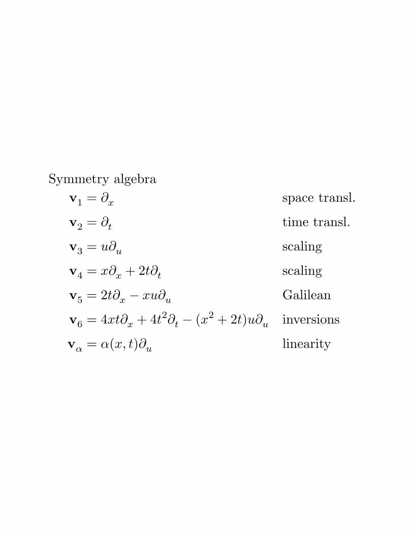
Symmetry algebra

v1 = ∂x space transl.

v2 = ∂t time transl.

v3 = u∂u scaling

v4 = x∂x + 2t∂t scaling

v5 = 2t∂x − xu∂u Galilean

v6 = 4xt∂x + 4t2∂t − (x2 + 2t)u∂u inversions

vα = α(x, t)∂u linearity

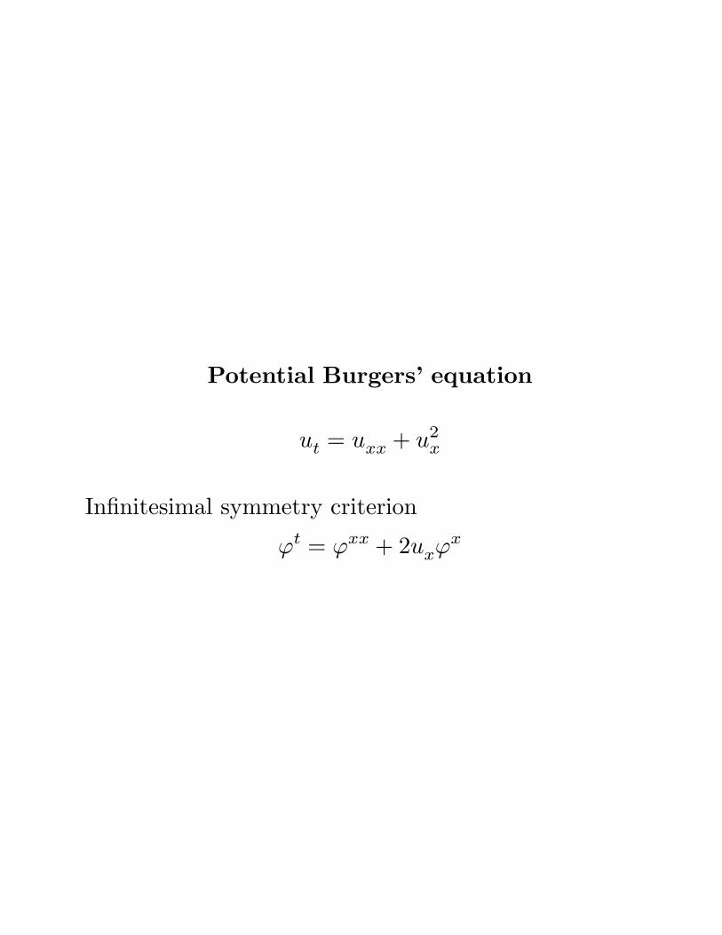
Potential Burgers’ equation

ut = uxx + u2x

Infinitesimal symmetry criterion

ϕt = ϕxx + 2uxϕx

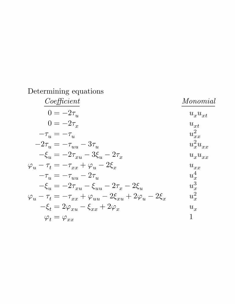
Determining equations

Coefficient Monomial

0 = −2τu uxuxt

0 = −2τx uxt

−τu = −τu u2xx

−2τu = −τuu − 3τu u2xuxx

−ξu = −2τxu − 3ξu − 2τx uxuxx

ϕu − τt = −τxx + ϕu − 2ξx uxx

−τu = −τuu − 2τu u4x

−ξu = −2τxu − ξuu − 2τx − 2ξu u3x

ϕu − τt = −τxx + ϕuu − 2ξxu + 2ϕu − 2ξx u2x

−ξt = 2ϕxu − ξxx + 2ϕx ux

ϕt = ϕxx 1

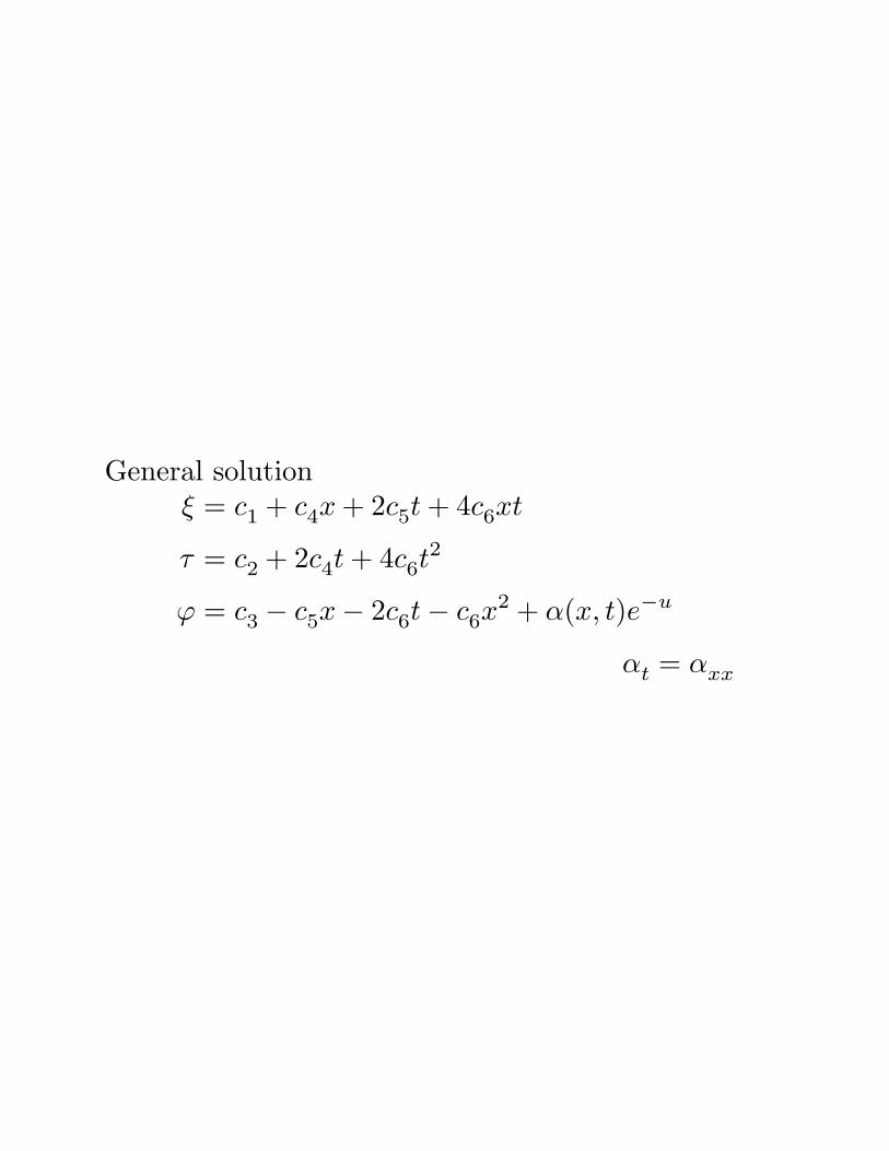
General solutionξ = c1 + c4x + 2c5t + 4c6xt

τ = c2 + 2c4t + 4c6t2

ϕ = c3 − c5x − 2c6t − c6x2 + α(x, t)e−u

αt = αxx

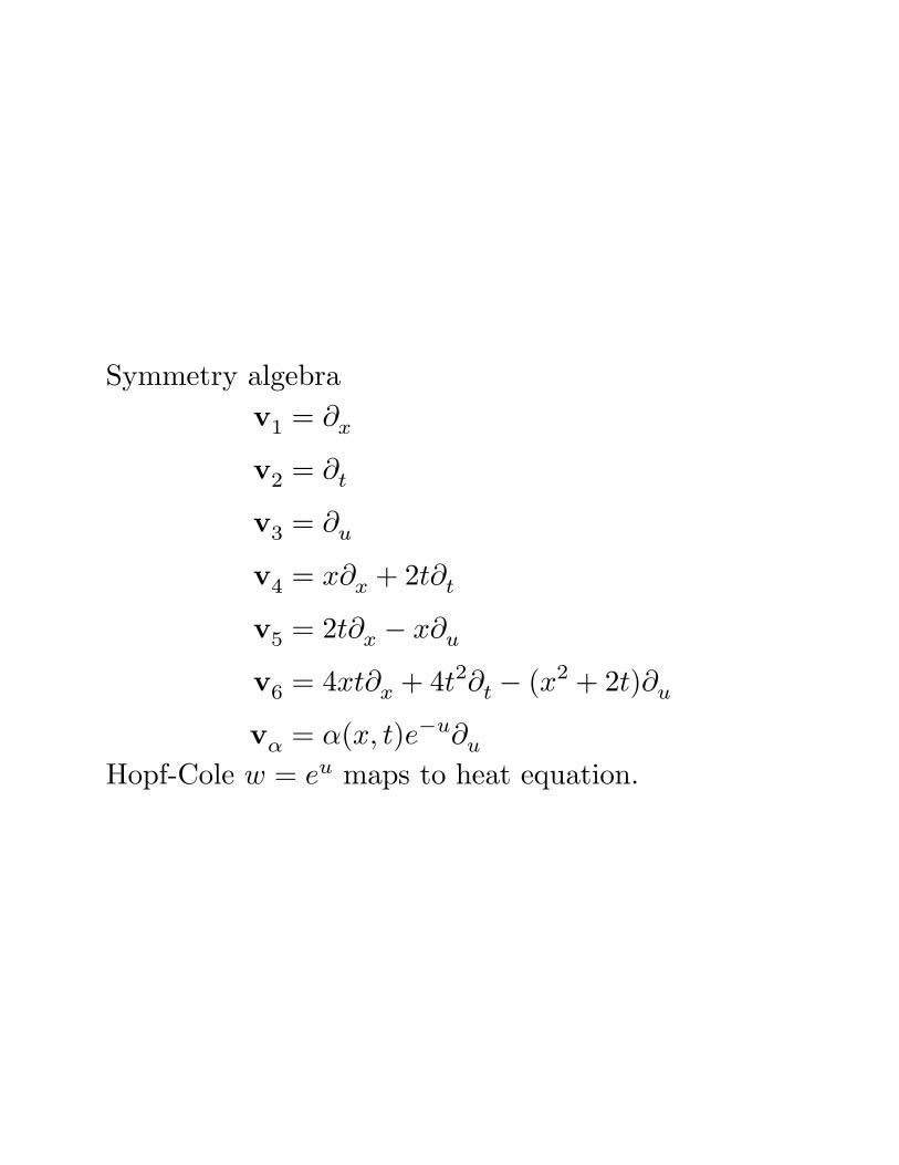
Symmetry algebra

v1 = ∂x

v2 = ∂t

v3 = ∂u

v4 = x∂x + 2t∂t

v5 = 2t∂x − x∂u

v6 = 4xt∂x + 4t2∂t − (x2 + 2t)∂u

vα = α(x, t)e−u∂u

Hopf-Cole w = eu maps to heat equation.

Symmetry–Based Solution Methods

Ordinary Differential Equations

• Lie’s method

• Solvable groups

• Variational and Hamiltonian systems

• Potential symmetries

• Exponential symmetries

• Generalized symmetries

Partial Differential Equations

• Group-invariant solutions

• Non-classical method

• Weak symmetry groups

• Clarkson-Kruskal method

• Partially invariant solutions

• Differential constraints

• Nonlocal Symmetries

• Separation of Variables

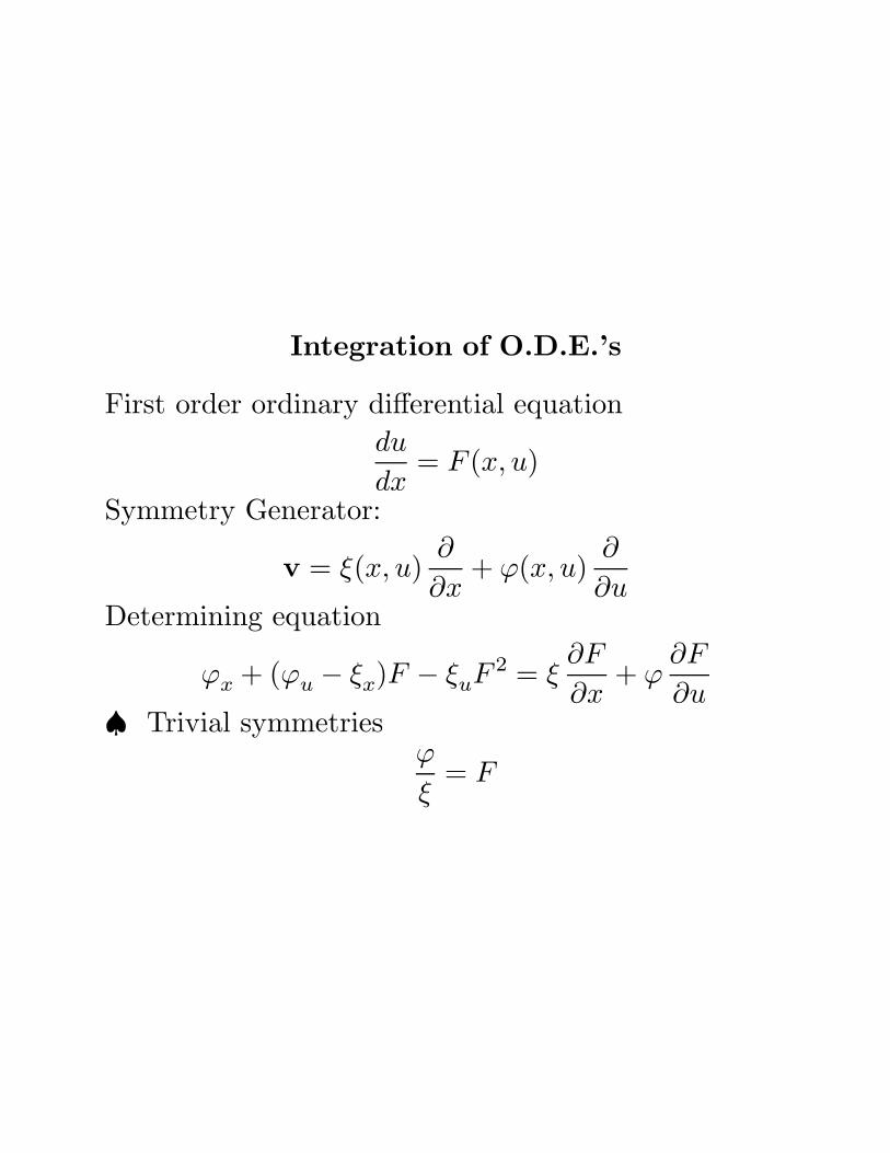
Integration of O.D.E.’s

First order ordinary differential equation

du

dx= F (x, u)

Symmetry Generator:

v = ξ(x, u)∂

∂x+ ϕ(x, u)

∂

∂uDetermining equation

ϕx + (ϕu − ξx)F − ξuF 2 = ξ∂F

∂x+ ϕ

∂F

∂u♠ Trivial symmetries

ϕ

ξ= F

Method 1: Rectify the vector field.

v|(x0,u0)6= 0

Introduce new coordinates

y = η(x, u) w = ζ(x, u)

near (x0, u0) so that

v =∂

∂wThese satisfy first order p.d.e.’s

ξ ηx + ϕ ηu = 0 ξ ζx + ϕ ζu = 1

Solution by method of characteristics:

dx

ξ(x, u)=

du

ϕ(x, u)=

dt

1

The equation in the new coordinates will be invariantif and only if it has the form

dw

dy= h(y)

and so can clearly be integrated by quadrature.

Method 2: Integrating Factor

If v = ξ ∂x + ϕ ∂u is a symmetry for

P (x, u) dx + Q(x, u) du = 0

then

R(x, u) =1

ξ P + ϕ Q

is an integrating factor.

♠ Ifϕ

ξ= − P

Q

then the integratimg factor is trivial. Also, rectificationof the vector field is equivalent to solving the originalo.d.e.

Higher Order Ordinary Differential Equations

∆(x, u(n)) = 0

If we know a one-parameter symmetry group

v = ξ(x, u)∂

∂x+ ϕ(x, u)

∂

∂uthen we can reduce the order of the equation by 1.

Method 1: Rectify v = ∂w. Then the equation isinvariant if and only if it does not depend on w:

∆(y, w′, . . . , wn) = 0

Set v = w′ to reduce the order.

Method 2: Differential invariants.

h[pr(n) g · (x, u(n)) ] = h(x, u(n)), g ∈ G

Infinitesimal criterion: pr v(h) = 0.

Proposition. If η, ζ are nth order differential invari-ants, then

dη

dζ=

Dxη

Dxζ

is an (n + 1)st order differential invariant.

Corollary. Let

y = η(x, u), w = ζ(x, u, u′)

be the independent first order differential invariants

for G. Any nth order o.d.e. admitting G as a symmetrygroup can be written in terms of the differentialinvariants y, w, dw/dy, . . . , dn−1w/dyn−1.

In terms of the differential invariants, the nth ordero.d.e. reduces to

∆(y, w(n−1)) = 0

For each solution w = g(y) of the reduced equation, wemust solve the auxiliary equation

ζ(x, u, u′) = g[η(x, u)]

to find u = f(x). This first order equation admits G asa symmetry group and so can be integrated as before.

Multiparameter groups

• G - r-dimensional Lie group.

Assume pr(r) G acts regularly with r dimensionalorbits.

Independent rth order differential invariants:

y = η(x, u(r)) w = ζ(x, u(r))

Independent nth order differential invariants:

y, w,dw

dy, . . . ,

dn−rw

dyn−r.

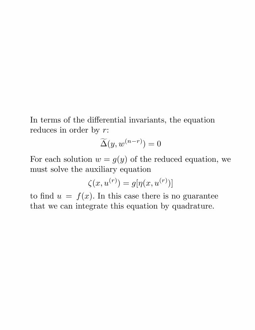
In terms of the differential invariants, the equationreduces in order by r:

∆(y, w(n−r)) = 0

For each solution w = g(y) of the reduced equation, wemust solve the auxiliary equation

ζ(x, u(r)) = g[η(x, u(r))]

to find u = f(x). In this case there is no guaranteethat we can integrate this equation by quadrature.

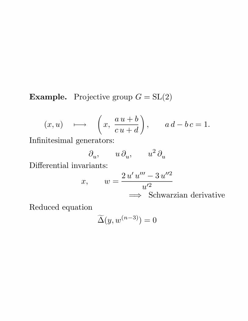
Example. Projective group G = SL(2)

(x, u) 7−→(

x,a u + b

c u + d

), a d − b c = 1.

Infinitesimal generators:

∂u, u ∂u, u2 ∂u

Differential invariants:

x, w =2 u′ u′′′ − 3 u′′2

u′2

=⇒ Schwarzian derivative

Reduced equation

∆(y, w(n−3)) = 0

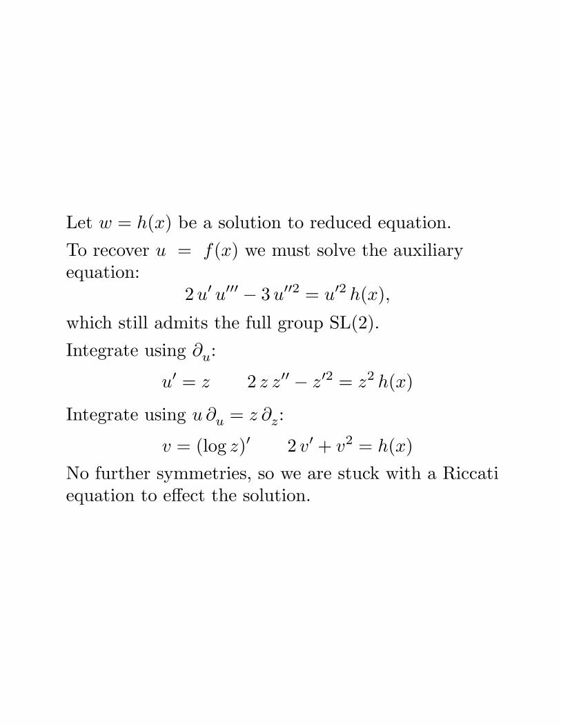
Let w = h(x) be a solution to reduced equation.

To recover u = f(x) we must solve the auxiliaryequation:

2 u′ u′′′ − 3 u′′2 = u′2 h(x),

which still admits the full group SL(2).

Integrate using ∂u:

u′ = z 2 z z′′ − z′2 = z2 h(x)

Integrate using u ∂u = z ∂z:

v = (log z)′ 2 v′ + v2 = h(x)

No further symmetries, so we are stuck with a Riccatiequation to effect the solution.

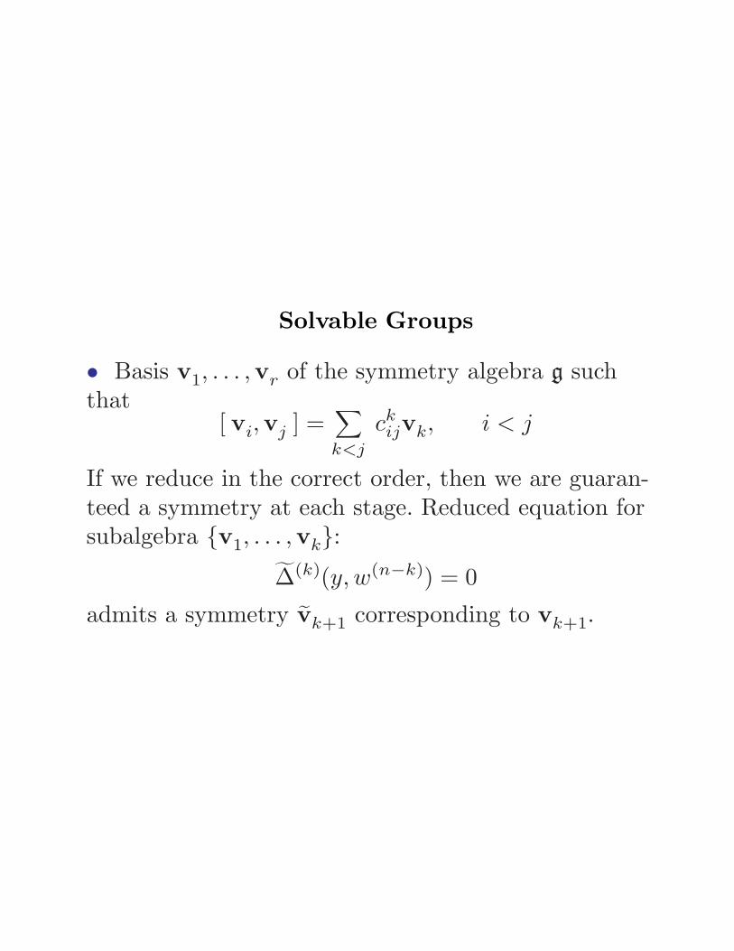
Solvable Groups

• Basis v1, . . . ,vr of the symmetry algebra g suchthat

[ vi,vj ] =∑

k<j

ckijvk, i < j

If we reduce in the correct order, then we are guaran-teed a symmetry at each stage. Reduced equation forsubalgebra v1, . . . ,vk:

∆(k)(y, w(n−k)) = 0

admits a symmetry vk+1 corresponding to vk+1.

Theorem. (Bianchi) If an nth order o.d.e. has a(regular) r-parameter solvable symmetry group, thenits solutions can be found by quadrature from those ofthe (n − r)th order reduced equation.

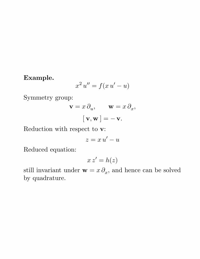
Example.x2 u′′ = f(x u′ − u)

Symmetry group:

v = x ∂u, w = x ∂x,

[ v,w ] = −v.

Reduction with respect to v:

z = x u′ − u

Reduced equation:

x z′ = h(z)

still invariant under w = x ∂x, and hence can be solvedby quadrature.

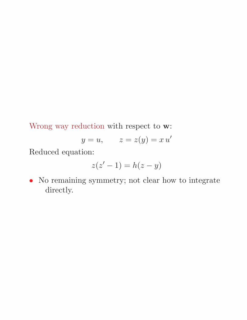
Wrong way reduction with respect to w:

y = u, z = z(y) = x u′

Reduced equation:

z(z′ − 1) = h(z − y)

• No remaining symmetry; not clear how to integratedirectly.

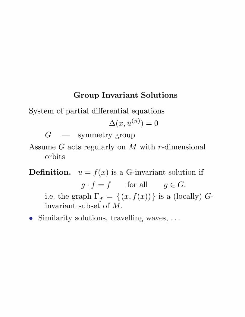
Group Invariant Solutions

System of partial differential equations

∆(x, u(n)) = 0

G — symmetry group

Assume G acts regularly on M with r-dimensionalorbits

Definition. u = f(x) is a G-invariant solution if

g · f = f for all g ∈ G.

i.e. the graph Γf = (x, f(x)) is a (locally) G-invariant subset of M .

• Similarity solutions, travelling waves, . . .

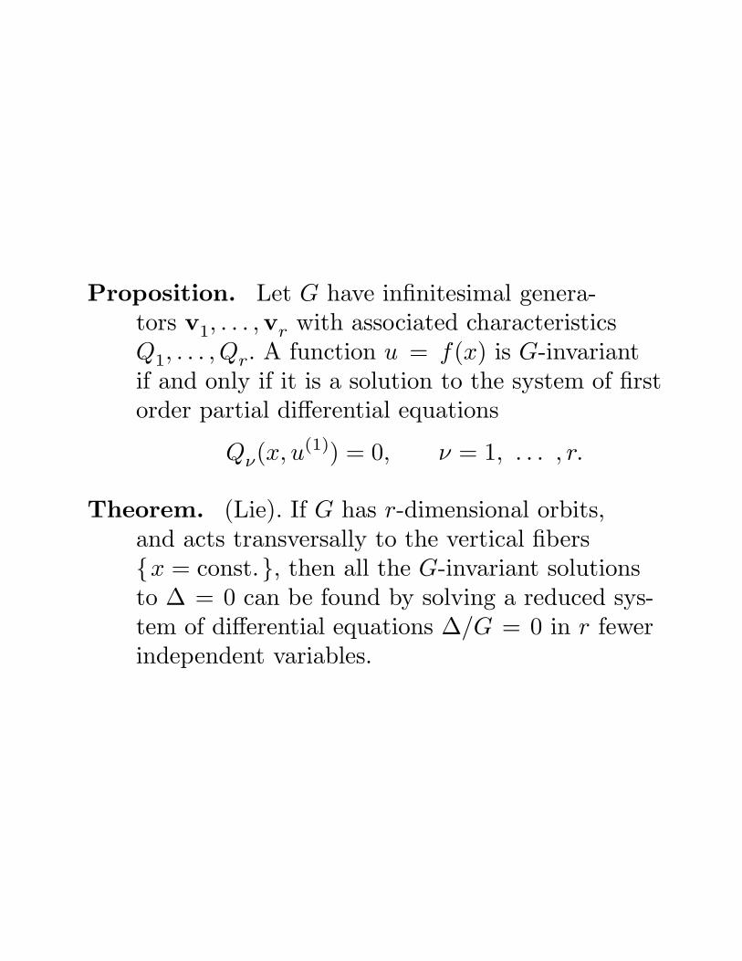
Proposition. Let G have infinitesimal genera-tors v1, . . . ,vr with associated characteristicsQ1, . . . , Qr. A function u = f(x) is G-invariantif and only if it is a solution to the system of firstorder partial differential equations

Qν(x, u(1)) = 0, ν = 1, . . . , r.

Theorem. (Lie). If G has r-dimensional orbits,and acts transversally to the vertical fibersx = const., then all the G-invariant solutionsto ∆ = 0 can be found by solving a reduced sys-tem of differential equations ∆/G = 0 in r fewerindependent variables.

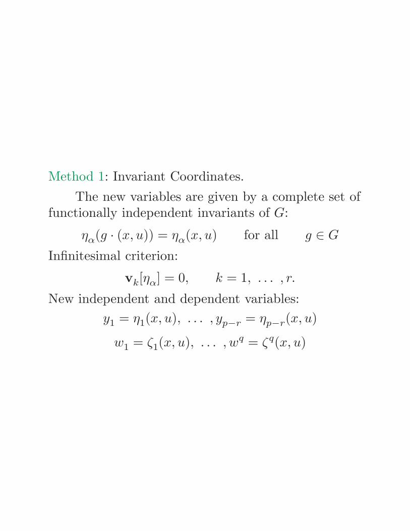
Method 1: Invariant Coordinates.

The new variables are given by a complete set offunctionally independent invariants of G:

ηα(g · (x, u)) = ηα(x, u) for all g ∈ G

Infinitesimal criterion:

vk[ηα] = 0, k = 1, . . . , r.

New independent and dependent variables:

y1 = η1(x, u), . . . , yp−r = ηp−r(x, u)

w1 = ζ1(x, u), . . . , wq = ζq(x, u)

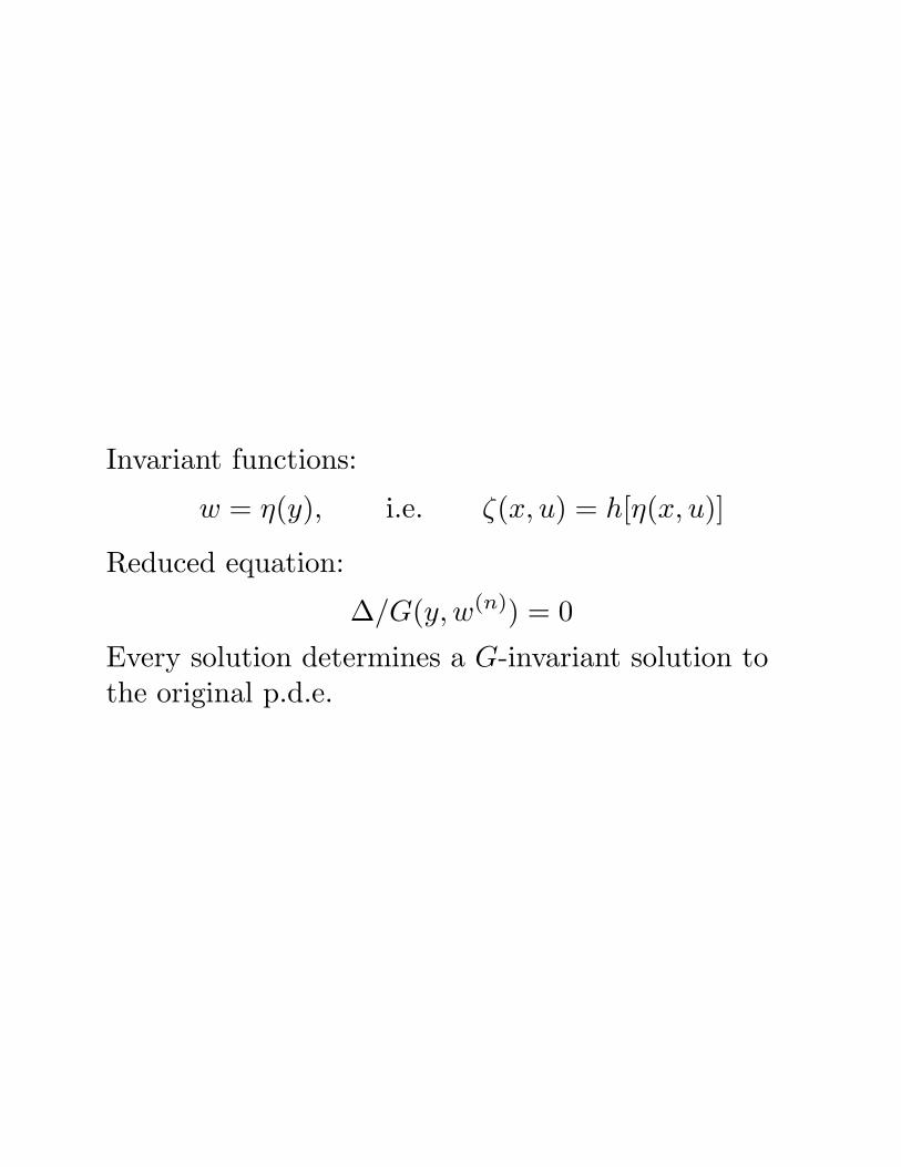
Invariant functions:

w = η(y), i.e. ζ(x, u) = h[η(x, u)]

Reduced equation:

∆/G(y, w(n)) = 0

Every solution determines a G-invariant solution tothe original p.d.e.

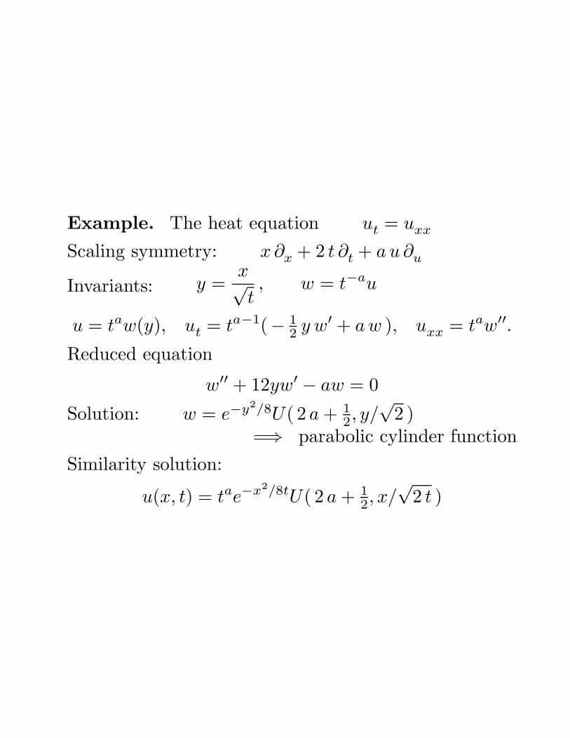
Example. The heat equation ut = uxx

Scaling symmetry: x ∂x + 2 t ∂t + a u ∂u

Invariants: y =x√t, w = t−au

u = taw(y), ut = ta−1(− 12 y w′ + a w ), uxx = taw′′.

Reduced equation

w′′ + 12yw′ − aw = 0

Solution: w = e−y2/8U( 2 a + 12, y/

√2 )

=⇒ parabolic cylinder function

Similarity solution:

u(x, t) = tae−x2/8tU( 2 a + 12, x/

√2 t )

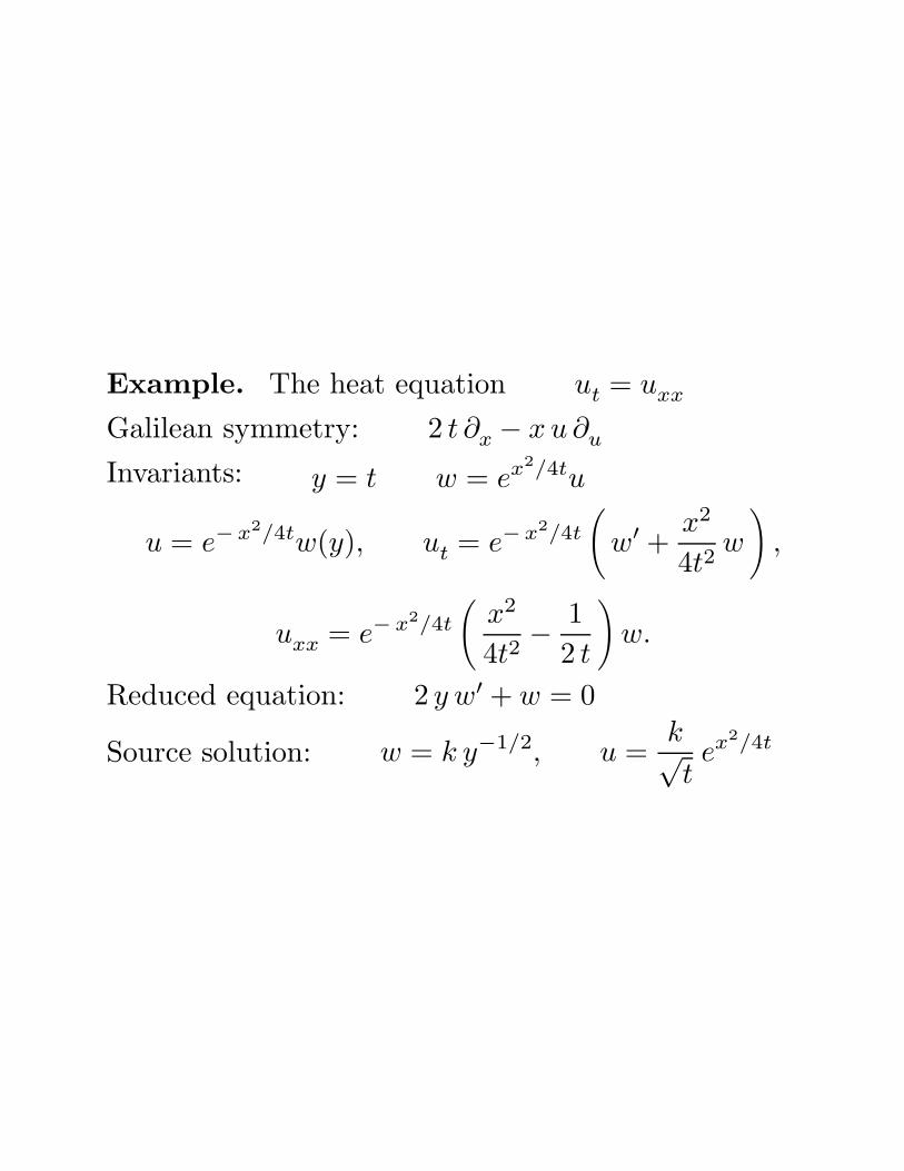
Example. The heat equation ut = uxx

Galilean symmetry: 2 t ∂x − x u ∂u

Invariants: y = t w = ex2/4tu

u = e−x2/4tw(y), ut = e−x2/4t

(w′ +

x2

4t2w

),

uxx = e− x2/4t

(x2

4t2− 1

2 t

)w.

Reduced equation: 2 y w′ + w = 0

Source solution: w = k y−1/2, u =k√tex2/4t

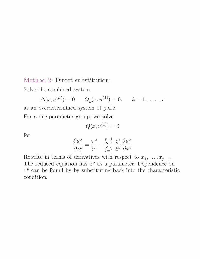
Method 2: Direct substitution:

Solve the combined system

∆(x, u(n)) = 0 Qk(x, u(1)) = 0, k = 1, . . . , r

as an overdetermined system of p.d.e.

For a one-parameter group, we solve

Q(x, u(1)) = 0

for∂uα

∂xp=

ϕα

ξn−

p−1∑

i=1

ξi

ξp

∂uα

∂xi

Rewrite in terms of derivatives with respect to x1, . . . , xp−1.The reduced equation has xp as a parameter. Dependence onxp can be found by by substituting back into the characteristiccondition.

Classification of invariant solutions

Let G be the full symmetry group of the system ∆ = 0. LetH ⊂ G be a subgroup. If u = f(x) is an H-invariant solution,and g ∈ G is another group element, then f = g·f is an invariantsolution for the conjugate subgroup H = g · H · g−1.

• Classification of subgroups of G under conjugation.

• Classification of subalgebras of g under the adjoint action.

• Exploit symmetry of the reduced equation

Non-Classical Method

=⇒ Bluman and Cole

Here we require not invariance of the original partial differentialequation, but rather invariance of the combined system

∆(x, u(n)) = 0 Qk(x, u(1)) = 0, k = 1, . . . , r

• Nonlinear determining equations.

• Most solutions derived using this approach come from ordi-nary group invariance anyway.

Weak (Partial) Symmetry Groups

Here we require invariance of

∆(x, u(n)) = 0 Qk(x, u(1)) = 0, k = 1, . . . , r

and all the associated integrability conditions

• Every group is a weak symmetry group.

• Every solution can be derived in this way.

• Compatibility of the combined system?

• Overdetermined systems of partial differential equations.

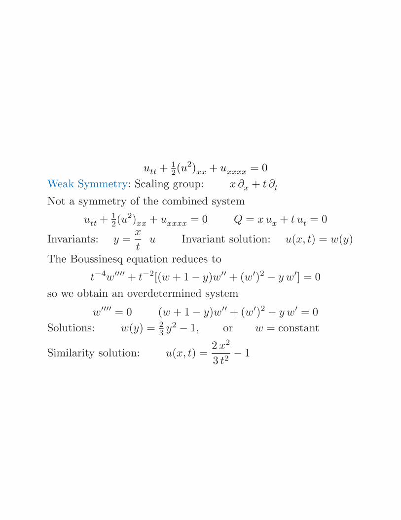
The Boussinesq Equation

utt + 12(u

2)xx + uxxxx = 0

Classical symmetry group:

v1 = ∂x v2 = ∂t v3 = x∂x + 2 t ∂t − 2u ∂u

For the scaling group

−Q = xux + 2 t ut + 2u = 0

Invariants:

y =x√t

w = t u u =1

tw

(x√t

)

Reduced equation:

w′′′′ + 12 (w2)′′ + 1

4 y2w′′ + 74 y w′ + 2w = 0

utt + 12(u

2)xx + uxxxx = 0

Group classification:

v1 = ∂x v2 = ∂t v3 = x∂x + 2 t ∂t − 2u ∂u

Note:

Ad(εv3)v1 = eε v1 Ad(εv3)v2 = e2 ε v2

Ad(δ v1 + εv2)v3 = v3 − δ v1 − εv2

so the one-dimensional subalgebras are classified by:

v3 v1 v2 v1 + v2 v1 − v2and we only need to determine solutions invariant underthese particular subgroups to find the most general group-invariant solution.

utt + 12(u

2)xx + uxxxx = 0

Non-classical: Galilean group

v = t ∂x + ∂t − 2 t ∂u

Not a symmetry, but the combined system

utt + 12(u

2)xx + uxxxx = 0 −Q = t ux + ut + 2 t = 0

does admit v as a symmetry. Invariants:

y = x − 12 t2, w = u + t2, u(x, t) = w(y) − t2

Reduced equation:

w′′′′ + ww′′ + (w′)2 − w′ + 2 = 0

utt + 12(u

2)xx + uxxxx = 0

Weak Symmetry: Scaling group: x∂x + t ∂t

Not a symmetry of the combined system

utt + 12(u

2)xx + uxxxx = 0 Q = xux + t ut = 0

Invariants: y =x

tu Invariant solution: u(x, t) = w(y)

The Boussinesq equation reduces to

t−4w′′′′ + t−2[(w + 1 − y)w′′ + (w′)2 − y w′] = 0

so we obtain an overdetermined system

w′′′′ = 0 (w + 1 − y)w′′ + (w′)2 − y w′ = 0

Solutions: w(y) = 23 y2 − 1, or w = constant

Similarity solution: u(x, t) =2 x2

3 t2− 1

Symmetries andConservation Laws

Variational problems

L[u ] =∫

ΩL(x, u(n)) dx

Euler-Lagrange equations

∆ = E(L) = 0

Euler operator (variational derivative)

Eα(L) =δL

δuα=∑

J

(−D)J ∂L

∂uαJ

Theorem. (Null Lagrangians)

E(L) ≡ 0 if and only if L = Div P

Theorem. The system ∆ = 0 is the Euler-Lagrangeequations for some variational problem if and only ifthe Frechet derivative D∆ is self-adjoint:

D∗∆ = D∆.

=⇒ Helmholtz conditions

Frechet derivative

Given P (x, u(n)), its Frechet derivative or formallinearization is the differential operator DP definedby

DP [w ] =d

dεP [u + εw ]

∣∣∣∣∣ε = 0

Example.P = uxxx + uux

DP = D3x + uDx + ux

Adjoint (formal)

D =∑

J

AJDJ D∗ =∑

J

(−D)J · AJ

Integration by parts formula:

P DQ = QD∗P + Div A

where A depends on P, Q.

Conservation Laws

Definition. A conservation law of a system of partialdifferential equations is a divergence expression

Div P = 0

which vanishes on all solutions to the system.

P = (P1(x, u(k)), . . . , Pp(x, u(k)))

=⇒ The integral ∫P · dS

is path (surface) independent.

If one of the coordinates is time, a conservation lawtakes the form

DtT + Div X = 0

T — conserved density X — flux

By the divergence theorem,∫

ΩT (x, t, u(k)) dx)

∣∣∣∣b

t=a=∫ b

a

∫

ΩX · dS dt

depends only on the boundary behavior of the solution.

• If the flux X vanishes on ∂Ω, then∫Ω T dx is

conserved (constant).

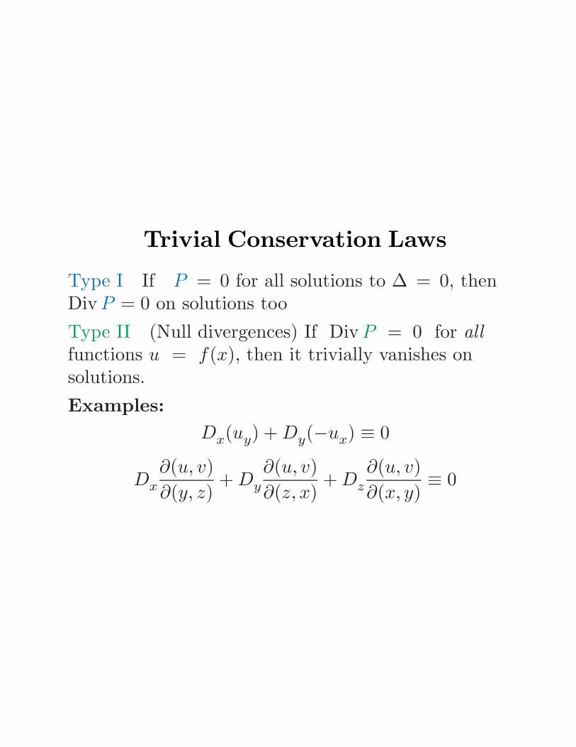
Trivial Conservation Laws

Type I If P = 0 for all solutions to ∆ = 0, thenDiv P = 0 on solutions too

Type II (Null divergences) If Div P = 0 for all

functions u = f(x), then it trivially vanishes onsolutions.

Examples:

Dx(uy) + Dy(−ux) ≡ 0

Dx

∂(u, v)

∂(y, z)+ Dy

∂(u, v)

∂(z, x)+ Dz

∂(u, v)

∂(x, y)≡ 0

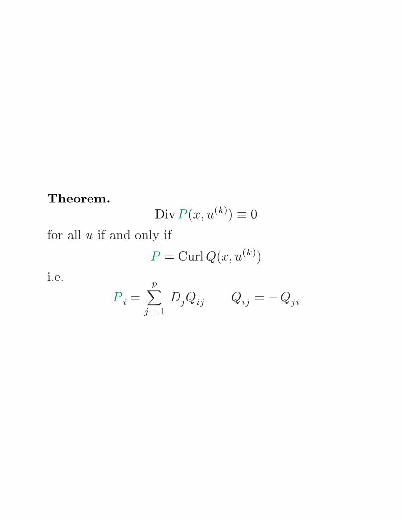
Theorem.Div P (x, u(k)) ≡ 0

for all u if and only if

P = Curl Q(x, u(k))

i.e.

P i =p∑

j =1

DjQij Qij = −Qji

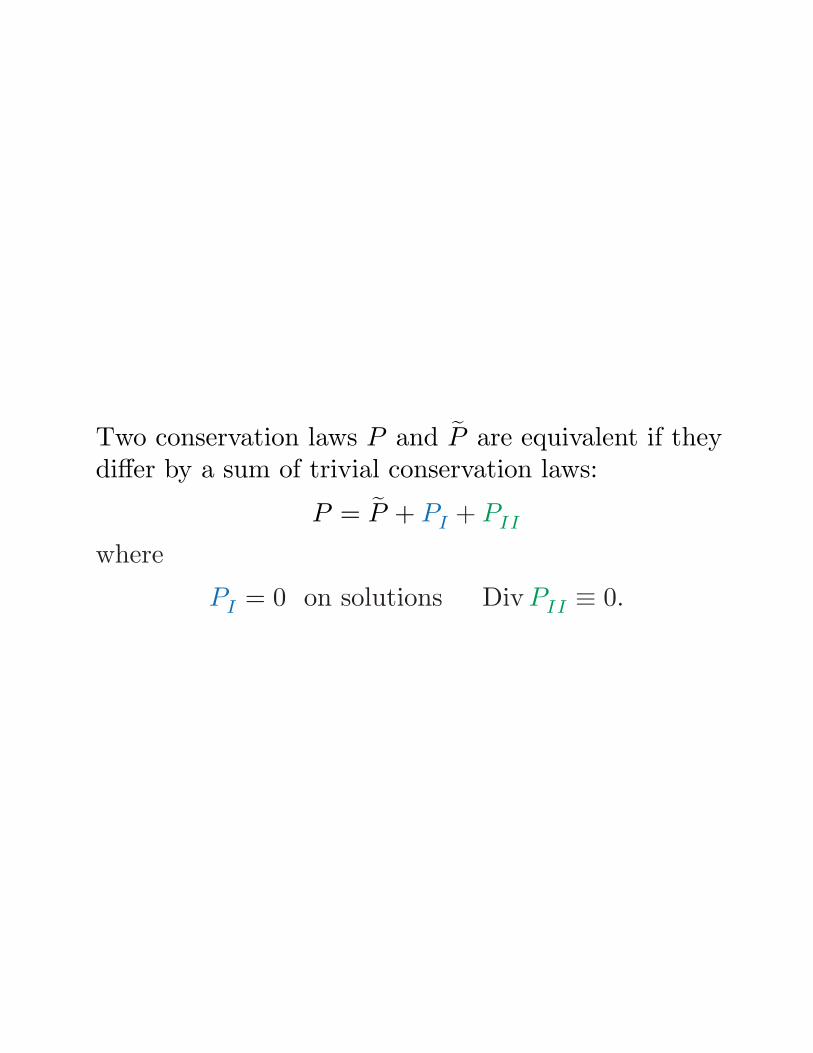
Two conservation laws P and P are equivalent if theydiffer by a sum of trivial conservation laws:

P = P + PI + PII

where

PI = 0 on solutions Div PII ≡ 0.

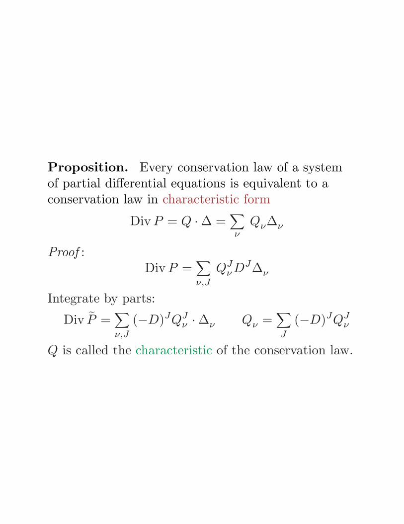
Proposition. Every conservation law of a systemof partial differential equations is equivalent to aconservation law in characteristic form

Div P = Q · ∆ =∑

νQν∆ν

Proof :Div P =

∑

ν,J

QJνDJ∆ν

Integrate by parts:

Div P =∑

ν,J

(−D)JQJν · ∆ν Qν =

∑

J

(−D)JQJν

Q is called the characteristic of the conservation law.

Theorem. Q is the characteristic of a conservationlaw for ∆ = 0 if and only if

D∗∆Q + D∗

Q∆ = 0.

Proof :

0 = E(Div P ) = E(Q · ∆) = D∗∆Q + D∗

Q∆

Normal Systems

A characteristic is trivial if it vanishes on solutions.Two characteristics are equivalent if they differ by atrivial one.

Theorem. Let ∆ = 0 be a normal system ofpartial differential equations. Then there is a one-to-one correspondence between (equivalence classes of)nontrivial conservation laws and (equivalence classesof) nontrivial characteristics.

Variational Symmetries

Definition. A (restricted) variational symmetry isa transformation (x, u) = g · (x, u) which leaves thevariational problem invariant:

∫

ΩL(x, u(n)) dx =

∫

ΩL(x, u(n)) dx

Infinitesimal criterion:

pr v(L) + L Div ξ = 0

Theorem. If v is a variational symmetry, then it is asymmetry of the Euler-Lagrange equations.

⋆ ⋆ But not conversely!

Noether’s Theorem (Weak version). If v generatesa one-parameter group of variational symmetries of avariational problem, then the characteristic Q of v isthe characteristic of a conservation law of the Euler-Lagrange equations:

Div P = Q E(L)

Elastostatics∫

W (x,∇u) dx — stored energy

x, u ∈ Rp, p = 2, 3

Frame indifference

u 7−→ R u + a, R ∈ SO(p)

Conservation laws = path independent integrals:

Div P = 0.

1. Translation invariance

Pi =∂W

∂uαi

=⇒ Euler-Lagrange equations

2. Rotational invariance

Pi = uαi

∂W

∂uβj

− uβi

∂W

∂uαj

3. Homogeneity : W = W (∇u) x 7−→ x + a

Pi =p∑

α=1

uαj

∂W

∂uαi

− δijW

=⇒ Energy-momentum tensor

4. Isotropy : W (∇u · Q) = W (∇u) Q ∈ SO(p)

Pi =p∑

α=1

(xjuαk − xkuα

j )∂W

∂uαi

+ (δijx

k − δikx

j)W

5. Dilation invariance : W (λ∇u) = λnW (∇u)

Pi =n − p

n

p∑

α,j =1

(uαδij − xjuα

j )∂W

∂uαi

+ xiW

5A. Divergence identity

Div P = p W

Pi =p∑

j =1

(uαδij − xjuα

j )∂W

∂uαi

+ xiW

=⇒ Knops/Stuart, Pohozaev, Pucci/Serrin

Generalized Vector Fields

Allow the coefficients of the infinitesimal generator todepend on derivatives of u:

v =p∑

i=1

ξi(x, u(k))∂

∂xi+

q∑

α=1

ϕα(x, u(k))∂

∂uα

Characteristic :

Qα(x, u(k)) = ϕα −p∑

i=1

ξiuαi

Evolutionary vector field:

vQ =q∑

α=1

Qα(x, u(k))∂

∂uα

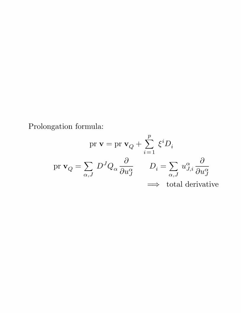
Prolongation formula:

pr v = pr vQ +p∑

i=1

ξiDi

pr vQ =∑

α,J

DJQα

∂

∂uαJ

Di =∑

α,J

uαJ,i

∂

∂uαJ

=⇒ total derivative

Generalized Flows

• The one-parameter group generated by an evolu-tionary vector field is found by solving the Cauchyproblem for an associated system of evolutionequations

∂uα

∂ε= Qα(x, u(n)) u|ε=0 = f(x)

Example. v =∂

∂xgenerates the one-parameter

group of translations:

(x, y, u) 7−→ (x + ε, y, u)

Evolutionary form:

vQ = −ux

∂

∂xCorresponding group:

∂u

∂ε= −ux

Solution

u = f(x, y) 7−→ u = f(x − ε, y)

Generalized Symmetries

of Differential Equations

Determining equations :

pr v(∆) = 0 whenever ∆ = 0

For totally nondegenerate systems, this is equivalent to

pr v(∆) = D∆ =∑

νDν∆ν

⋆ v is a generalized symmetry if and only if itsevolutionary form vQ is.

• A generalized symmetry is trivial if its characteristicvanishes on solutions to ∆. Two symmetries are equivalentif their evolutionary forms differ by a trivial symmetry.

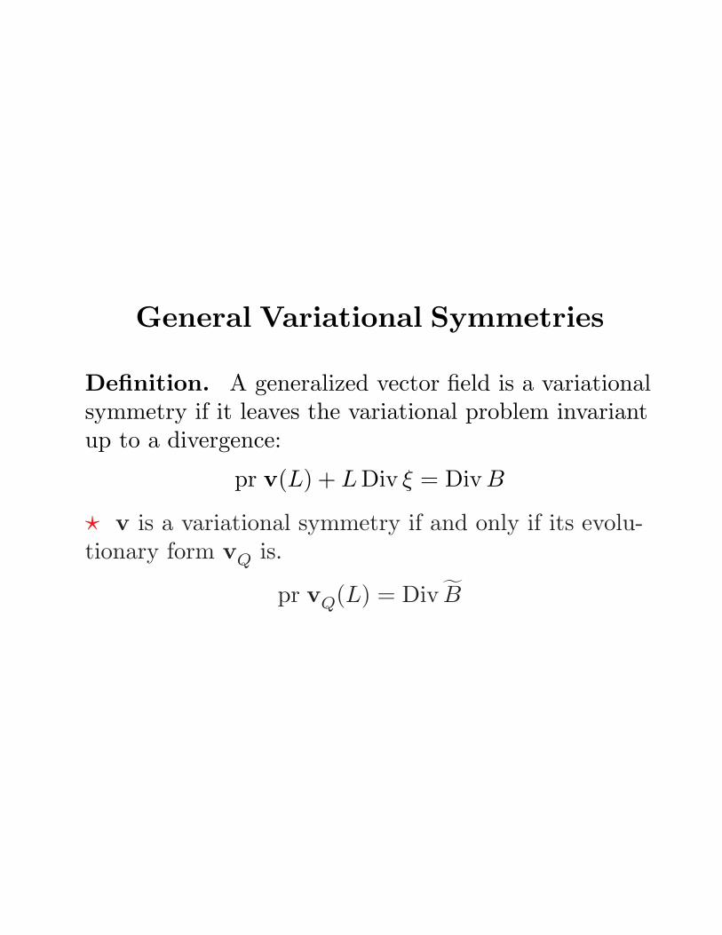
General Variational Symmetries

Definition. A generalized vector field is a variationalsymmetry if it leaves the variational problem invariantup to a divergence:

pr v(L) + L Div ξ = Div B

⋆ v is a variational symmetry if and only if its evolu-tionary form vQ is.

pr vQ(L) = Div B

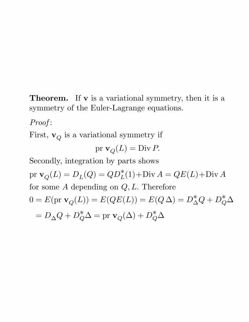
Theorem. If v is a variational symmetry, then it is asymmetry of the Euler-Lagrange equations.

Proof :

First, vQ is a variational symmetry if

pr vQ(L) = Div P.

Secondly, integration by parts shows

pr vQ(L) = DL(Q) = QD∗L(1)+Div A = QE(L)+Div A

for some A depending on Q, L. Therefore

0 = E(pr vQ(L)) = E(QE(L)) = E(Q ∆) = D∗∆Q + D∗

Q∆

= D∆Q + D∗Q∆ = pr vQ(∆) + D∗

Q∆

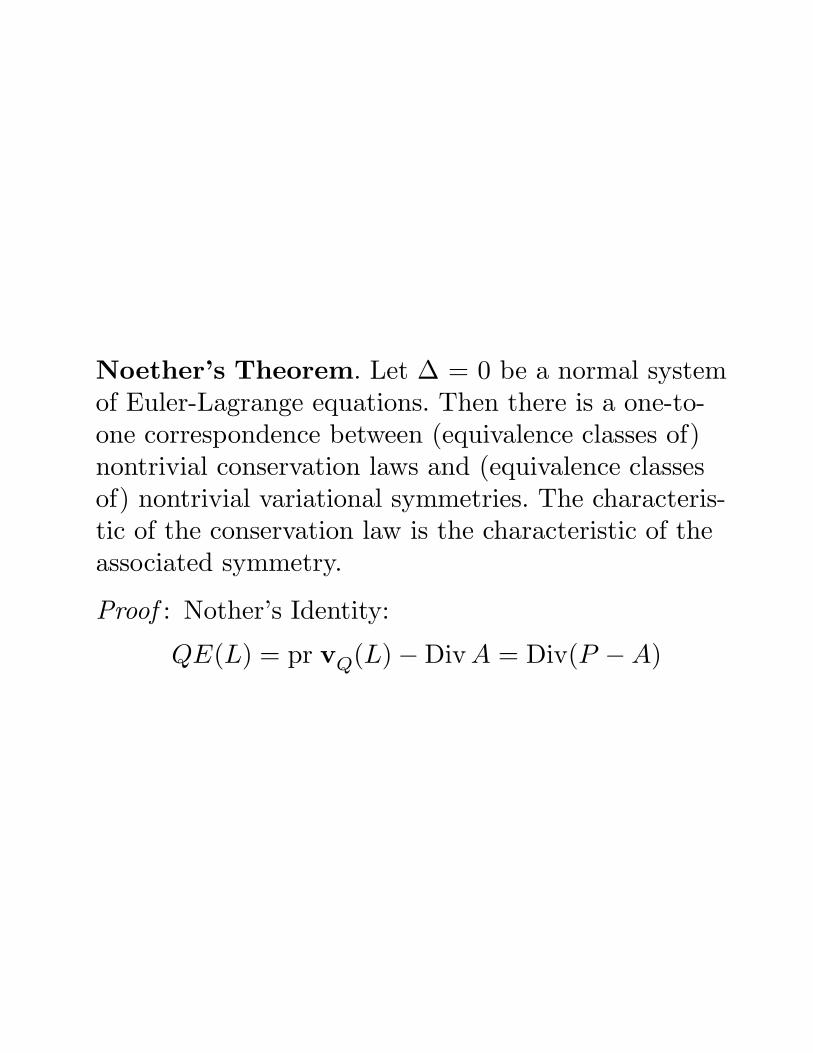
Noether’s Theorem. Let ∆ = 0 be a normal systemof Euler-Lagrange equations. Then there is a one-to-one correspondence between (equivalence classes of)nontrivial conservation laws and (equivalence classesof) nontrivial variational symmetries. The characteris-tic of the conservation law is the characteristic of theassociated symmetry.

Proof : Nother’s Identity:

QE(L) = pr vQ(L) − Div A = Div(P − A)

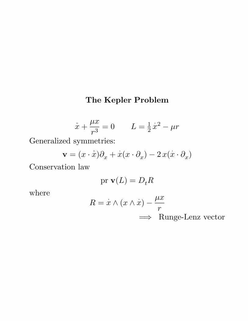
The Kepler Problem

x +µx

r3= 0 L = 1

2

x2 − µr

Generalized symmetries:

v = (x ·

x)∂x +

x(x · ∂x) − 2 x(

x · ∂x)

Conservation law

pr v(L) = DtR

whereR =

x ∧ (x ∧

x) − µx

r=⇒ Runge-Lenz vector

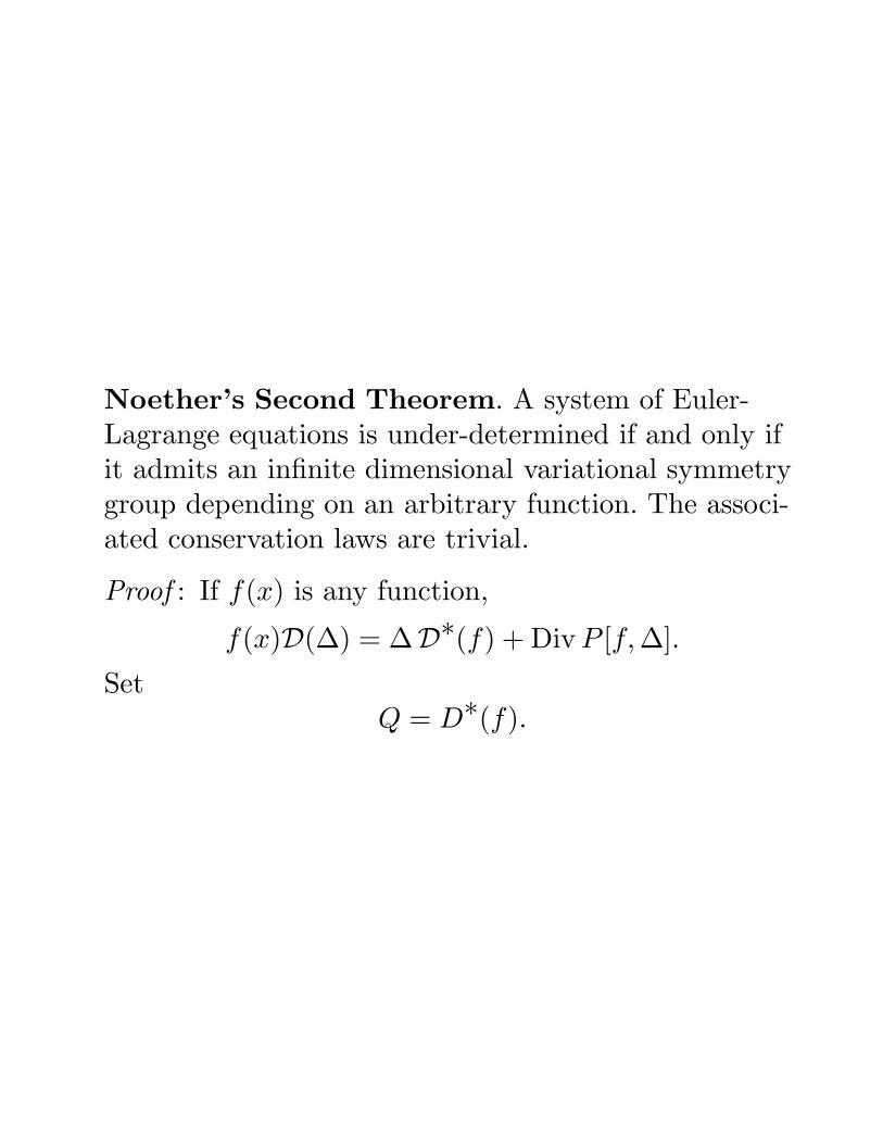
Noether’s Second Theorem. A system of Euler-Lagrange equations is under-determined if and only ifit admits an infinite dimensional variational symmetrygroup depending on an arbitrary function. The associ-ated conservation laws are trivial.

Proof : If f(x) is any function,

f(x)D(∆) = ∆D∗(f) + Div P [f, ∆].

SetQ = D∗(f).

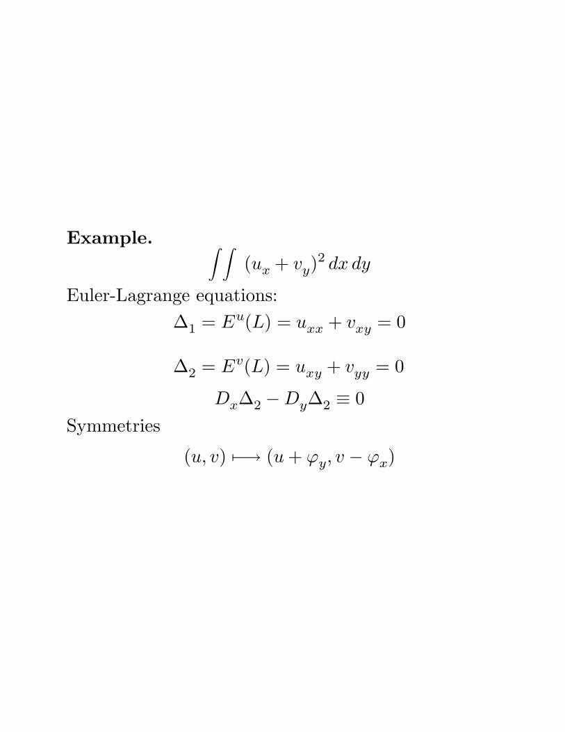
Example. ∫ ∫(ux + vy)

2 dx dy

Euler-Lagrange equations:

∆1 = Eu(L) = uxx + vxy = 0

∆2 = Ev(L) = uxy + vyy = 0

Dx∆2 − Dy∆2 ≡ 0

Symmetries

(u, v) 7−→ (u + ϕy, v − ϕx)