
Sur un Problème de Monge de Transport Optimal de Masse · Sur un Probl eme de Monge de Transport...
24
Sur un Probl` eme de Monge de Transport Optimal de Masse Noureddine Igbida LAMFA CNRS-UMR 6140 Universit´ e de Picardie Jules Verne, 80000 Amiens Limoges, 25 Mars 2010 MODE 2010, Limoges Noureddine Igbida Sur un Probl` eme de Monge de Transport Optimal de Masse
Transcript of Sur un Problème de Monge de Transport Optimal de Masse · Sur un Probl eme de Monge de Transport...

Sur un Probleme de Monge de TransportOptimal de Masse
Noureddine Igbida
LAMFA CNRS-UMR 6140Universite de Picardie Jules Verne, 80000 Amiens
Limoges, 25 Mars 2010MODE 2010, Limoges
Noureddine Igbida Sur un Probleme de Monge de Transport Optimal de Masse
Monge problem
Y
f^+ f^−
t
=t#f^+
x y=t(x)
X
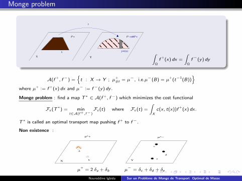
∫Ω
f +(x) dx =
∫Ω
f−(y) dy
A(f +, f−) =
t : X → Y ; µ+
#t = µ−, i.e.µ−(B) = µ
+(t−1(B))
where µ+ := f +(x) dx and µ− := f−(y) dy .
Monge problem : find a map T∗ ∈ A(f +, f−) which minimizes the cost functional
Fc (T∗) = mint∈A(f +,f−)
Fc (t) where Fc (t) =
∫X
c(x, t(x))f +(x) dx.
T∗ is called an optimal transport map pushing f + to f−.
Non existence :
d
X Y
µ^+ µ^−
e
a
b
c
µ+ = 2 δa + δb µ
− = δc + δd + δe
Noureddine Igbida Sur un Probleme de Monge de Transport Optimal de Masse
Monge-Kantorovich problem
µ^−
X
Y
µ
µ^+
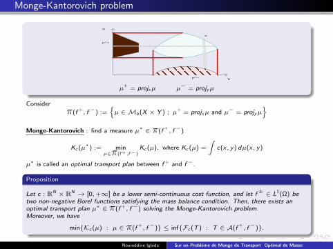
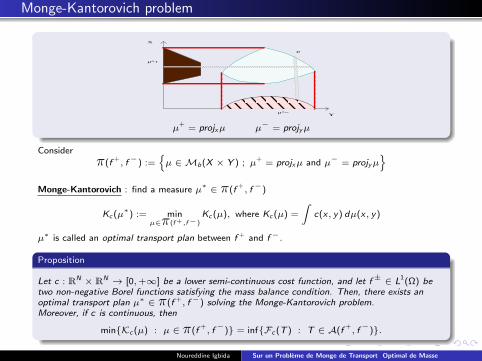
µ+ = projxµ µ
− = projyµ
Consider
π(f +, f−) :=
µ ∈ Mb(X × Y ) ; µ+ = projxµ and µ− = projyµ
Monge-Kantorovich : find a measure µ∗ ∈ π(f +
, f−)
Kc (µ∗) := minµ∈π(f +,f−)
Kc (µ), where Kc (µ) =
∫c(x, y) dµ(x, y)
µ∗ is called an optimal transport plan between f + and f−.
Proposition
Let c : RN × RN → [0,+∞] be a lower semi-continuous cost function, and let f± ∈ L1(Ω) betwo non-negative Borel functions satisfying the mass balance condition. Then, there exists anoptimal transport plan µ∗ ∈ π(f +, f−) solving the Monge-Kantorovich problem.Moreover, we have
minKc (µ) : µ ∈ π(f +, f−) ≤ infFc (T ) : T ∈ A(f +
, f−).
Noureddine Igbida Sur un Probleme de Monge de Transport Optimal de Masse
Monge-Kantorovich problem
µ^−
X
Y
µ
µ^+
µ+ = projxµ µ
− = projyµ
Consider
π(f +, f−) :=
µ ∈ Mb(X × Y ) ; µ+ = projxµ and µ− = projyµ
Monge-Kantorovich : find a measure µ∗ ∈ π(f +
, f−)
Kc (µ∗) := minµ∈π(f +,f−)
Kc (µ), where Kc (µ) =
∫c(x, y) dµ(x, y)
µ∗ is called an optimal transport plan between f + and f−.
Proposition
Let c : RN × RN → [0,+∞] be a lower semi-continuous cost function, and let f± ∈ L1(Ω) betwo non-negative Borel functions satisfying the mass balance condition. Then, there exists anoptimal transport plan µ∗ ∈ π(f +, f−) solving the Monge-Kantorovich problem.Moreover, if c is continuous, then
minKc (µ) : µ ∈ π(f +, f−) = infFc (T ) : T ∈ A(f +
, f−).
Noureddine Igbida Sur un Probleme de Monge de Transport Optimal de Masse
Kantorovich dual problem
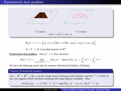
f^+f^−
Y
X
f +(x)u(x) ...... f−(x)v(y)u(x) + v(y) ≤ c(x, y)
Φc (f +, f−) :=
(u, v) ∈ L1(Ω)× L1(Ω) : u(x) + v(y) ≤ c(x, y)
X ∪ Y ⊆ Ω a bounded domain of RN
Kantorovich dual problem : find (u∗, v∗) that maximize
D(u∗, v∗) = max(u,v)∈Φc (f +,f−)
D(u, v) where D(u, v) :=
∫X
u f + +
∫Y
v f−
We have the following result (see for instance [Ambrosio-Pratelli] or [Villani]).
Theorem (Kantorovich duality)
Let c : RN × RN → [0,+∞] be a lower semi-continuous cost function, and let f± ∈ L1(Ω) betwo non-negative Borel functions satisfying the mass balance condition. Then,
minKc (µ) : µ ∈ π(f +, f−) = supD(u, v) : (u, v) ∈ Φc (f +
, f−).
Noureddine Igbida Sur un Probleme de Monge de Transport Optimal de Masse
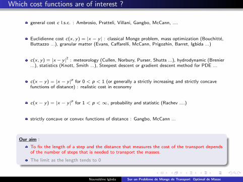
Which cost functions are of interest ?
general cost c l.s.c. : Ambrosio, Pratteli, Villani, Gangbo, McCann, ....
Euclidienne cost c(x, y) = |x − y | : classical Monge problem, mass optimization (Bouchitte,Buttazzo ...), granular matter (Evans, Caffarelli, McCann, Prigozhin, Barret, Igbida ...)
c(x, y) = |x − y |2 : meteorology (Cullen, Norbury, Purser, Shutts ...), hydrodynamic (Brenier...), statistics (Knott, Smith ...), Steepest descent or gradient descent method for PDE ...
c(x − y) = |x − y |p for 0 < p < 1 (or generally a strictly increasing and strictly concavefunctions of distance) : realistic cost in economy
c(x − y) = |x − y |p for 1 < p <∞, probability and statistic (Rachev ....)
strictly concave or convex functions of distance : Gangbo, McCann ...
Our aim :
To fix the length of a step and the distance that measures the cost of the transport dependsof the number of steps that is needed to transport the masses.
The limit as the length tends to 0
Noureddine Igbida Sur un Probleme de Monge de Transport Optimal de Masse
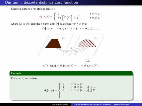
Our aim : discrete distance cost function
Discrete distance for step of size ε :
dε(x, y) =
0 if x = y ,
ε([[|x−y|ε
]]+ 1)
if x 6= y .
where |.| is the Euclidean norm and [[r ]] is defined for r > 0 by
[[r ]] := n, if n < r ≤ n + 1, n = 0, 1, 2, . . . .
x
f^+ f^−
epsilon
t_1
t_4
t_2t_3
dε(x, t1(x) = dε(x, t2(x) = ... = dε(x, t4(x)).
Example
For ε = 1, we obtain
d1(x, y) =
0 if x = y ,1 if 0 < |x − y | ≤ 1,2 if 1 < |x − y | ≤ 2,
.
.
.
Noureddine Igbida Sur un Probleme de Monge de Transport Optimal de Masse
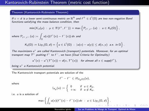
Kantorovich-Rubinstein Theorem (metric cost function)
Theorem (Kantorovich-Rubinstein Theorem)
If c = d is a lower semi-continuous metric on RN and f± ∈ L1(Ω) are two non-negative Borelfunctions satisfying the mass balance condition, then
minKd (µ) : µ ∈ π(f +, f−) = maxPf +,f− (u) : u ∈ Kd (Ω)
,
where Pf +,f− (u) :=
∫Ω
u(x)(f +(x)− f−(x)) dx and
Kd (Ω) := Lip1(Ω, d) =
u ∈ L1(Ω) : |u(x)− u(y)| ≤ d(x, y) a.e. in Ω.
The maximizers u∗ are called Kantorovich (transport) potentials. Moreover, for an optimal
transport map T∗ pushing f + to f−, we have (Dual Criteria for Optimality)
u∗(x)− u∗(T∗(x)) = d(x,T∗(x)) for almost all x ∈ supp(f +),
being u∗ a Kantorovich potential.
The Kantorovich transport potentials are solution of the
f + − f− ∈ ∂IKd (Ω)(u),
where
IKd(u) :=
0 if u ∈ Kd ,+∞ if u 6∈ Kd ,
i.e. u is a solution of
max
∫Ω
u(x)(f +(x)− f−(x)) dx : u ∈ Lip1(Ω, d)
.
Noureddine Igbida Sur un Probleme de Monge de Transport Optimal de Masse
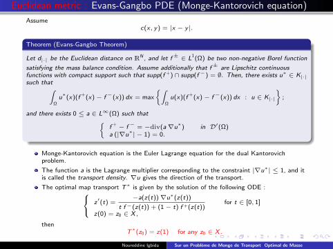
Euclidean metric : Evans-Gangbo PDE (Monge-Kantorovich equation)
Assumec(x, y) = |x − y |.
Theorem (Evans-Gangbo Theorem)
Let d|·| be the Euclidean distance on RN , and let f± ∈ L1(Ω) be two non-negative Borel function
satisfying the mass balance condition. Assume additionally that f± are Lipschitz continuousfunctions with compact support such that supp(f +)∩ supp(f−) = ∅. Then, there exists u∗ ∈ K|·|such that∫
Ω
u∗(x)(f +(x)− f−(x)) dx = max
∫Ω
u(x)(f +(x)− f−(x)) dx : u ∈ K|·|
;
and there exists 0 ≤ a ∈ L∞(Ω) such thatf + − f− = −div(a∇u∗) in D′(Ω)a (|∇u∗| − 1) = 0.
Monge-Kantorovich equation is the Euler Lagrange equation for the dual Kantorovichproblem.
The function a is the Lagrange multiplier corresponding to the constraint |∇u∗| ≤ 1, and itis called the transport density. ∇u gives the direction of the transport.
The optimal map transport T∗ is given by the solution of the following ODE : z′(t) =−a(z(t))∇u∗(z(t))
t f−(z(t)) + (1− t) f +(z(t))for t ∈ [0, 1]
z(0) = z0 ∈ X ,
thenT∗(z0) = z(1) for any z0 ∈ X .
Noureddine Igbida Sur un Probleme de Monge de Transport Optimal de Masse
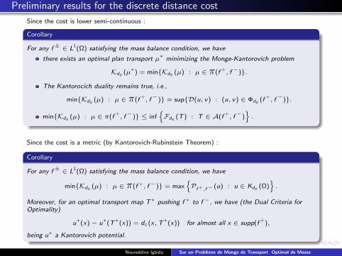
Preliminary results for the discrete distance cost
Since the cost is lower semi-continuous :
Corollary
For any f± ∈ L1(Ω) satisfying the mass balance condition, we have
there exists an optimal plan transport µ∗ minimizing the Monge-Kantorovich problem
Kdε (µ∗) = minKdε (µ) : µ ∈ π(f +, f−).
The Kantorocich duality remains true, i.e.,
minKdε (µ) : µ ∈ π(f +, f−) = supD(u, v) : (u, v) ∈ Φdε (f +
, f−).
minKdε (µ) : µ ∈ π(f +, f−) ≤ inf
Fdε (T ) : T ∈ A(f +
, f−).
Since the cost is a metric (by Kantorovich-Rubinstein Theorem) :
Corollary
For any f± ∈ L1(Ω) satisfying the mass balance condition, we have
minKdε (µ) : µ ∈ π(f +, f−) = maxPf +,f− (u) : u ∈ Kdε (Ω)
.
Moreover, for an optimal transport map T∗ pushing f + to f−, we have (the Dual Criteria forOptimality)
u∗(x)− u∗(T∗(x)) = dε(x,T∗(x)) for almost all x ∈ supp(f +),
being u∗ a Kantorovich potential.
Noureddine Igbida Sur un Probleme de Monge de Transport Optimal de Masse
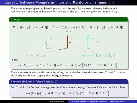
Equality between Monge’s infimun and Kantorovich’s minimum
The same example given by Pratelli proves that the equality between Monge’s infimun andKantorovich’s minimum is not true for the case of the cost function given by the metric d1 :
Example
R := (−1, y) : y ∈ [−1, 1], S := (0, y) : y ∈ [−1, 1], Q := (1, y) : y ∈ [−1, 1].
Q
0
1
−1
1
S
−1 x
y
R
f + := 2H1 S f− := H1 R +H1 Q
Then
minKd1(µ) : µ ∈ π(f +
, f−) = 2 < 4 ≤ infFd1
(T ) : T ∈ A(f +, f−)
.
The cause here is not the discontinuity of d1, but is the fact that the measures f + and f− are notabsolutely continuous respect the Lebesgue measure.
Theorem (Ig-Mazon-Toledo-Rossi,2010)
Let f± ∈ L1(Ω) be two non-negative Borel functions satisfying the mass balance condition. Then,
minKdε (µ) : µ ∈ π(f +, f−) = inf
Fdε (T ) : T ∈ A(f +
, f−).
Noureddine Igbida Sur un Probleme de Monge de Transport Optimal de Masse
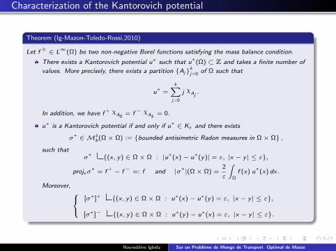
Characterization of the Kantorovich potential
Theorem (Ig-Mazon-Toledo-Rossi,2010)
Let f± ∈ L∞(Ω) be two non-negative Borel functions satisfying the mass balance condition.
There exists a Kantorovich potential u∗ such that u∗(Ω) ⊂ Z and takes a finite number of
values. More precisely, there exists a partition Ajkj=0 of Ω such that
u∗ =k∑
j=0
j χAj.
In addition, we have f + χA0
= f− χAk= 0.
u∗ is a Kantorovich potential if and only if u∗ ∈ Kε and there exists
σ∗ ∈ Ma
b(Ω× Ω) := bounded antisimetric Radon measures in Ω× Ω ,
such thatσ∗ (x, y) ∈ Ω× Ω : |u∗(x)− u∗(y)| = ε, |x − y | ≤ ε,
projxσ∗ = f + − f− =: f and |σ∗|(Ω× Ω) =
2
ε
∫Ω
f (x) u∗(x) dx.
Moreover, [σ∗]+ (x, y) ∈ Ω× Ω : u∗(x)− u∗(y) = ε, |x − y | ≤ ε,
[σ∗]− (x, y) ∈ Ω× Ω : u∗(y)− u∗(x) = ε, |x − y | ≤ ε.
Noureddine Igbida Sur un Probleme de Monge de Transport Optimal de Masse
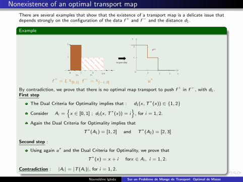
Nonexistence of an optimal transport map
There are several examples that show that the existence of a transport map is a delicate issue thatdepends strongly on the configuration of the data f + and f− and the distance d1.
Example
we prov ethat
0 2
1
L
1f^+ f^−
x
y
1
0 1 2 3
2
u^*
L=3
f + = L χ[0,1] f− = χ
[−L,0] u∗
By contradiction, we prove that there is no optimal map transport to push f + in f−, with d1.First step
The Dual Criteria for Optimality implies that : d1(x,T∗(x)) ∈ 1, 2
Consider Ai =
x ∈ [0, 1] ; d1(x,T∗(x)) = i, for i = 1, 2.
Again the Dual Criteria for Optimality implies that
T∗(A1) = [1, 2] and T∗(A2) = [2, 3]
Second step :
Using again u∗ and the Dual Criteria for Optimality, we prove that
T∗(x) = x + i forx ∈ Ai , i = 1, 2.
Contradiction : |Ai | = |T (Ai )|, for i = 1, 2.
Noureddine Igbida Sur un Probleme de Monge de Transport Optimal de Masse
Construction of an optimal plan transport
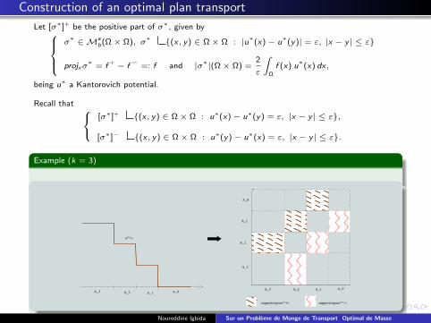
Let [σ∗]+ be the positive part of σ∗, given byσ∗ ∈ Ma
b(Ω× Ω), σ∗ (x, y) ∈ Ω× Ω : |u∗(x)− u∗(y)| = ε, |x − y | ≤ ε
projxσ∗ = f + − f− =: f and |σ∗|(Ω× Ω) =
2
ε
∫Ω
f (x) u∗(x) dx,
being u∗ a Kantorovich potential.
Recall that [σ∗]+ (x, y) ∈ Ω× Ω : u∗(x)− u∗(y) = ε, |x − y | ≤ ε,
[σ∗]− (x, y) ∈ Ω× Ω : u∗(y)− u∗(x) = ε, |x − y | ≤ ε.
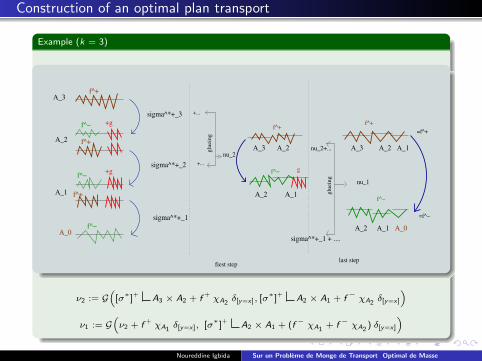
Example (k = 3)
support(sigma^*−)
A_3 A_2 A_0A_1
u^*+
A_0
A_0A_3
A_3
A_2
A_2
A_1
A_1
support(sigma^*+)
Noureddine Igbida Sur un Probleme de Monge de Transport Optimal de Masse
Construction of an optimal plan transport
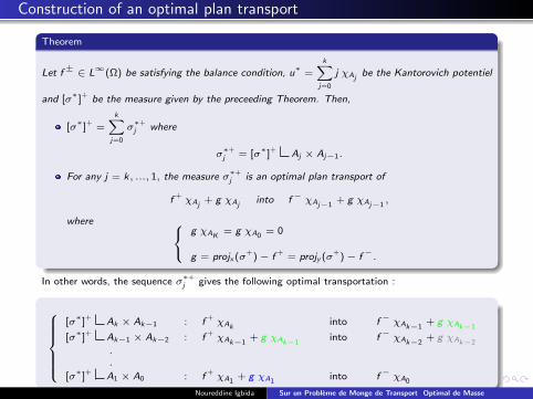
Theorem
Let f± ∈ L∞(Ω) be satisfying the balance condition, u∗ =k∑
j=0
j χAjbe the Kantorovich potentiel
and [σ∗]+ be the measure given by the preceeding Theorem. Then,
[σ∗]+ =k∑
j=0
σ∗+j where
σ∗+j = [σ∗]+ Aj × Aj−1.
For any j = k, ..., 1, the measure σ∗+j is an optimal plan transport of
f +χAj
+ g χAjinto f− χAj−1
+ g χAj−1,
where g χAK
= g χA0= 0
g = projx (σ+)− f + = projy (σ+)− f−.
In other words, the sequence σ∗+j gives the following optimal transportation :
[σ∗]+ Ak × Ak−1 : f +χAk
into f− χAk−1+ g χAk−1
[σ∗]+ Ak−1 × Ak−2 : f +χAk−1
+ g χAk−1into f− χAk−2
+ g χAk−2
.
.
[σ∗]+ A1 × A0 : f +χA1
+ g χA1into f− χA0
Noureddine Igbida Sur un Probleme de Monge de Transport Optimal de Masse
Construction of an optimal plan transport
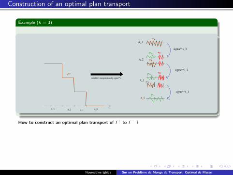
Example (k = 3)
f^−
A_3 A_2 A_0A_1
u^*detailled transportation by sigma^*+
A_3
A_2
A_1
A_0
f^+
+g
f^+
+g
f^+
sigma^*+_3
sigma^*+_2
sigma^*+_1
f^−
f^−
How to construct an optimal plan transport of f + to f− ?
Lemma (Gluing Lemma, Villani)
Let f1, f2, h be three positive measures in Ω. If µ1 ∈ π(f1, h) and µ2 ∈ π(h, f2), there exits ameasure G(µ1, µ2) ∈ π(f1, f2) such that
Kd (G(µ1, µ2)) ≤ Kd (µ1) +Kd (µ2).
Noureddine Igbida Sur un Probleme de Monge de Transport Optimal de Masse
Construction of an optimal plan transport
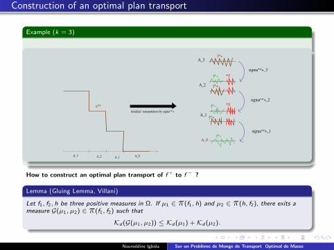
Example (k = 3)
f^−
A_3 A_2 A_0A_1
u^*detailled transportation by sigma^*+
A_3
A_2
A_1
A_0
f^+
+g
f^+
+g
f^+
sigma^*+_3
sigma^*+_2
sigma^*+_1
f^−
f^−
How to construct an optimal plan transport of f + to f− ?
Lemma (Gluing Lemma, Villani)
Let f1, f2, h be three positive measures in Ω. If µ1 ∈ π(f1, h) and µ2 ∈ π(h, f2), there exits ameasure G(µ1, µ2) ∈ π(f1, f2) such that
Kd (G(µ1, µ2)) ≤ Kd (µ1) +Kd (µ2).
Noureddine Igbida Sur un Probleme de Monge de Transport Optimal de Masse
Construction of an optimal plan transport
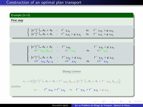
Example (k=3)
First step
[σ∗]+ A3 × A2 : f +
χA3to f− χA2
+ g χA2
[σ∗]+ A2 × A1 : f +χA2
+ g χA2to f− χA1
+ g χA1
[σ∗]+ A3 × A2 : f +
χA3f− χA2
+ g χA2
+f +χA2
δ[y=x] : +f +χA2
to +f +χA2
[σ∗]+ A2 × A1 : f +χA2
+ g χA2f− χA1
+ g χA1
+f− χA2δ[y=x] : +f− χA2
to +f− χA2
Gluing Lemma
ν2 := G(
[σ∗]+ A3 × A2 + f +χA2
δ[y=x], [σ∗]+ A2 × A1 + f− χA2δ[y=x]
)satisfies
ν2 : f +χA3
+ f +χA2
to f− χA1+ f− χA2
+ g χA1
Noureddine Igbida Sur un Probleme de Monge de Transport Optimal de Masse
Construction of an optimal plan transport
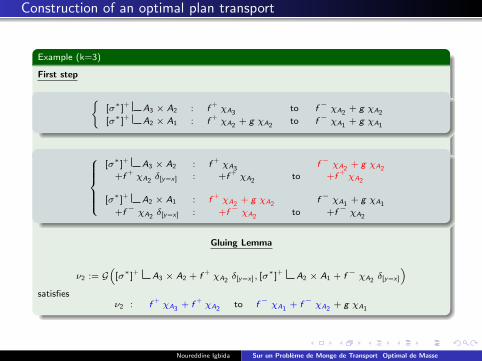
Example (k=3)
First step
[σ∗]+ A3 × A2 : f +
χA3to f− χA2
+ g χA2
[σ∗]+ A2 × A1 : f +χA2
+ g χA2to f− χA1
+ g χA1
[σ∗]+ A3 × A2 : f +
χA3f− χA2
+ g χA2
+f +χA2
δ[y=x] : +f +χA2
to +f +χA2
[σ∗]+ A2 × A1 : f +χA2
+ g χA2f− χA1
+ g χA1
+f− χA2δ[y=x] : +f− χA2
to +f− χA2
Gluing Lemma
ν2 := G(
[σ∗]+ A3 × A2 + f +χA2
δ[y=x], [σ∗]+ A2 × A1 + f− χA2δ[y=x]
)satisfies
ν2 : f +χA3
+ f +χA2
to f− χA1+ f− χA2
+ g χA1
Noureddine Igbida Sur un Probleme de Monge de Transport Optimal de Masse
Construction of an optimal plan transport
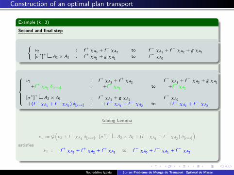
Example (k=3)
Second and final step
ν2 : f +
χA3+ f +
χA2to f− χA1
+ f− χA2+ g χA1
[σ∗]+ A2 × A1 : f +χA1
+ g χA1to f− χA0
ν2 : f +
χA3+ f +
χA2f− χA1
+ f− χA2+ g χA1
+f +χA1
δ[y=x] : +f +χA1
to +f +χA1
[σ∗]+ A2 × A1 : f +χA1
+ g χA1f− χA0
+(f− χA1+ f− χA2
) δ[y=x] : +f− χA1+ f− χA2
to +f− χA1+ f− χA2
Gluing Lemma
ν1 := G(ν2 + f +
χA1δ[y=x], [σ∗]+ A2 × A1 + (f− χA1
+ f− χA2) δ[y=x]
)satisfies
ν1 : f +χA3
+ f +χA2
+ f +χA1
to f− χA0+ f− χA1
+ f− χA2
Noureddine Igbida Sur un Probleme de Monge de Transport Optimal de Masse
Construction of an optimal plan transport
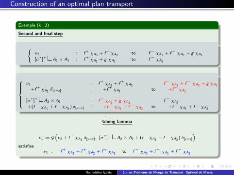
Example (k=3)
Second and final step
ν2 : f +
χA3+ f +
χA2to f− χA1
+ f− χA2+ g χA1
[σ∗]+ A2 × A1 : f +χA1
+ g χA1to f− χA0
ν2 : f +
χA3+ f +
χA2f− χA1
+ f− χA2+ g χA1
+f +χA1
δ[y=x] : +f +χA1
to +f +χA1
[σ∗]+ A2 × A1 : f +χA1
+ g χA1f− χA0
+(f− χA1+ f− χA2
) δ[y=x] : +f− χA1+ f− χA2
to +f− χA1+ f− χA2
Gluing Lemma
ν1 := G(ν2 + f +
χA1δ[y=x], [σ∗]+ A2 × A1 + (f− χA1
+ f− χA2) δ[y=x]
)satisfies
ν1 : f +χA3
+ f +χA2
+ f +χA1
to f− χA0+ f− χA1
+ f− χA2
Noureddine Igbida Sur un Probleme de Monge de Transport Optimal de Masse
Construction of an optimal plan transport
Example (k = 3)
=f^+
A_3
A_2
A_0
f^+
+g
f^+
+g
f^+
sigma^*+_3
sigma^*+_2
sigma^*+_1
f^−
f^−
f^−
+...
+...
A_1
g
f^+
f^−
f^+
f^−
A_3 A_2 A_1
A_2 A_1 A_0
A_3 A_2
A_2 A_1
nu_2 nu_2+...
nu_1
sigma^*+_1 + ....
fiest steplast step
glu
ein
g
glu
ein
g
=f^−
ν2 := G(
[σ∗]+ A3 × A2 + f +χA2
δ[y=x], [σ∗]+ A2 × A1 + f− χA2δ[y=x]
)ν1 := G
(ν2 + f +
χA1δ[y=x], [σ∗]+ A2 × A1 + (f− χA1
+ f− χA2) δ[y=x]
)Noureddine Igbida Sur un Probleme de Monge de Transport Optimal de Masse
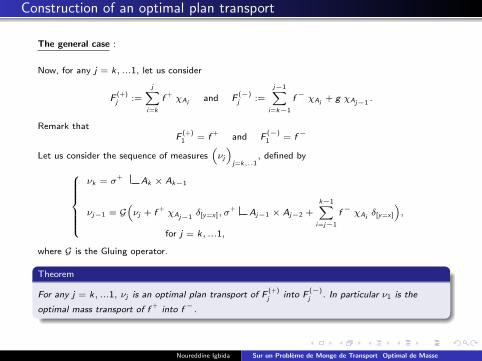
Construction of an optimal plan transport
The general case :
Now, for any j = k, ...1, let us consider
F(+)j :=
j∑i=k
f +χAi
and F(−)j :=
j−1∑i=k−1
f− χAi+ g χAj−1
.
Remark thatF
(+)1 = f + and F
(−)1 = f−
Let us consider the sequence of measures(νj
)j=k,..1
, defined by
νk = σ+ Ak × Ak−1
νj−1 = G(νj + f +
χAj−1δ[y=x], σ
+ Aj−1 × Aj−2 +
k−1∑i=j−1
f− χAiδ[y=x]
),
for j = k, ...1,
where G is the Gluing operator.
Theorem
For any j = k, ...1, νj is an optimal plan transport of F(+)j into F
(−)j . In particular ν1 is the
optimal mass transport of f + into f−.
Noureddine Igbida Sur un Probleme de Monge de Transport Optimal de Masse
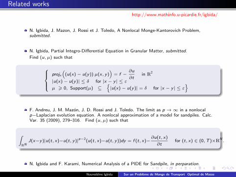
Related works
http://www.mathinfo.u-picardie.fr/igbida/
N. Igbida, J. Mazon, J. Rossi et J. Toledo, A Nonlocal Monge-Kantorovich Problem,submitted.
N. Igbida, Partial Integro-Differential Equation in Granular Matter, submitted.
Find (u, µ) such that
projx
((u(x)− u(y)) µ(x, y)
)= f −
∂u
∂tin R2
|u(x)− u(y)| ≤ δ for |x − y | ≤ εµ > 0, Support(µ) ⊆
|u(x)− u(y)| = δ for |x − y | ≤ ε
F. Andreu, J. M. Mazon, J. D. Rossi and J. Toledo. The limit as p →∞ in a nonlocalp−Laplacian evolution equation. A nonlocal approximation of a model for sandpiles. Calc.Var. 35 (2009), 279–316. Find (u, µ) such that
∫RN
J(x−y)|u(t, x)−u(t, y)|p−2(u(t, x)−u(t, y))dy = f (t, x)−∂u(t, x)
∂tfor (t, x) ∈ (0,T )×RN
.
N. Igbida and F. Karami, Numerical Analysis of a PIDE for Sandpile, in perparation.
Noureddine Igbida Sur un Probleme de Monge de Transport Optimal de Masse


![Radial-GelenklaGeR din iSO 12240-1 MaSSReihe G · lFd GelenklaGeR Produktkatalog 27 erfolgreich durch Präzision. Bezeichnung Hauptabmessungen Masse Tragzahlen Anschlussmaße d [mm]](https://static.fdocument.org/doc/165x107/5b5eb78b7f8b9a553d8d1ff3/radial-gelenklager-din-iso-12240-1-massreihe-g-lfd-gelenklager-produktkatalog.jpg)


![arxiv.org · arXiv:1501.07167v3 [math.CV] 29 Apr 2015 DEGENERATE COMPLEX MONGE-AMPERE FLOWS ON` STRICTLY PSEUDOCONVEX DOMAINS DO HOANG SON Abstract. We study the equation ˙u= logdet(uαβ¯)](https://static.fdocument.org/doc/165x107/5ed655ddce712b01aa66ed7c/arxivorg-arxiv150107167v3-mathcv-29-apr-2015-degenerate-complex-monge-ampere.jpg)