UNIVERSITY OF OSLODepartment of Informatics

Suppression of ∆ΣDAC QuantisationNoise by BandwidthAdaptationThesis in partialfulfillment of therequirements for thedegree of Cand. Scient.

Jørgen AndreasMichaelsen

May 15, 2006

contents

1 Introduction 91.1 Related work . . . . . . . . . . . . . . . . . . . . . . . . . . . . 10

1.2 Thesis outline . . . . . . . . . . . . . . . . . . . . . . . . . . . 11

2 Background 132.1 Lowpass oversampling ∆Σ digital to analogue conversion . 13

2.1.1 Interpolation filter . . . . . . . . . . . . . . . . . . . . 14

2.1.2 ∆Σ modulator . . . . . . . . . . . . . . . . . . . . . . . 15

2.1.3 D/A conversion . . . . . . . . . . . . . . . . . . . . . 19

2.1.4 Reconstruction filter . . . . . . . . . . . . . . . . . . . 19

2.1.5 Performance . . . . . . . . . . . . . . . . . . . . . . . . 19

2.2 Tunable filter . . . . . . . . . . . . . . . . . . . . . . . . . . . . 22

2.2.1 Switched-capacitor basics . . . . . . . . . . . . . . . . 22

2.2.2 Switched-capacitor filter structures . . . . . . . . . . 24

2.2.3 Tunable switched-capacitor filters . . . . . . . . . . . 25

2.3 Signal analysis . . . . . . . . . . . . . . . . . . . . . . . . . . . 27

2.3.1 The short time Fourier transform . . . . . . . . . . . 27

2.3.2 Wavelets . . . . . . . . . . . . . . . . . . . . . . . . . . 28

2.3.3 Subband coded signals . . . . . . . . . . . . . . . . . 30

3 Theory 333.1 Implementation . . . . . . . . . . . . . . . . . . . . . . . . . . 33

3.1.1 Signal analysis . . . . . . . . . . . . . . . . . . . . . . 33

3.1.2 Tunable reconstruction filter . . . . . . . . . . . . . . 35

3.1.3 Assembling the system . . . . . . . . . . . . . . . . . 37

3.2 Performance gain . . . . . . . . . . . . . . . . . . . . . . . . . 37

4 Simulation 414.1 Simulation model implementation . . . . . . . . . . . . . . . 41

4.2 Experimental Setup . . . . . . . . . . . . . . . . . . . . . . . . 42

4.3 Results obtained from a synthetic input signal . . . . . . . . 43

4.4 Results obtained from audio data input . . . . . . . . . . . . 47

4.5 Summary of measured results . . . . . . . . . . . . . . . . . . 48

4

5 Conclusion 535.1 Conclusion . . . . . . . . . . . . . . . . . . . . . . . . . . . . . 53

5.2 Future work . . . . . . . . . . . . . . . . . . . . . . . . . . . . 54

A Source code 55A.1 Octave scripts . . . . . . . . . . . . . . . . . . . . . . . . . . . 55

A.2 Simulator . . . . . . . . . . . . . . . . . . . . . . . . . . . . . . 57

A.2.1 Top-level . . . . . . . . . . . . . . . . . . . . . . . . . . 57

A.2.2 MPEG audio parser . . . . . . . . . . . . . . . . . . . 61

A.2.3 ∆Σ modulator . . . . . . . . . . . . . . . . . . . . . . . 67

A.2.4 Reconstruction filter . . . . . . . . . . . . . . . . . . . 68

list of figures

1.1 Basic outline of the proposed noise reduction scheme . . . . 10

2.1 High-level overview of a ∆Σ DAC . . . . . . . . . . . . . . . 13

2.2 Interpolation filter . . . . . . . . . . . . . . . . . . . . . . . . 14

2.3 Cascaded interpolation filter (N = 4) . . . . . . . . . . . . . . 15

2.4 Polyphase interpolation filter . . . . . . . . . . . . . . . . . . 16

2.5 ∆Σ modulator . . . . . . . . . . . . . . . . . . . . . . . . . . . 16

2.6 Plot of noise shaping gain as a function of angular frequency 18

2.7 A basic switched-capacitor resistor approximation . . . . . . 23

2.8 The charge programming circuit from [1] . . . . . . . . . . . 26

2.9 The Daubechies wavelet with three vanishing moments . . . 29

2.10 Wavelet analysis implemented by a filter bank . . . . . . . . 29

2.11 Subband encoder and decoder system . . . . . . . . . . . . . 31

2.12 MPEG-1 audio decoding overview . . . . . . . . . . . . . . . 32

3.1 Input signal analysis with decoupling to reconstruction filter 34

3.2 Wrapping a static bandwidth ∆Σ DAC . . . . . . . . . . . . 35

3.3 Full integration with the ∆Σ DAC . . . . . . . . . . . . . . . 36

3.4 Relative SNR improvement as a function of bandwidth . . . 38

4.1 A time domain comparison of the 1 kHz output signal . . . 44

4.2 A frequency domain presentation of the first time window . 45

4.3 A time domain comparison of the 2 kHz output signal . . . 47

4.4 Interpolated output from the MPEG audio decoder . . . . . 49

4.5 Unfiltered output from the ∆Σ modulator . . . . . . . . . . . 49

4.6 Output reconstructed with a static cutoff frequency filter . . 50

4.7 Output reconstructed with a dynamic cutoff frequency filter 50

4.8 Interpolated output from the MPEG audio decoder . . . . . 51

4.9 Unfiltered output from the ∆Σ modulator . . . . . . . . . . . 51

4.10 Output reconstructed with a static cutoff frequency filter . . 52

4.11 Output reconstructed with a dynamic cutoff frequency filter 52

A.1 Frequency response of two reconstruction filters . . . . . . . 72

This page is intentionally left blank

preface

Please find enclosed, a thesis in partial fulfillment of the requirementsfor the degree of Cand. Scient., respectfully submitted for your perusal.

I would like to take this opportunity to thank my supervisor, Dag T.Wisland, for his skillful guidance during the execution of this work. Iwould also like to thank my parents, Karin and Oddbjørn, for their kindsupport throughout, and Maja for encouraging me to finish. Thank youall for your patience. Thanks are also due to Viktor S. Wold Eide, FrankEliassen, and Hans Ole Rafaelsen for giving me the opportunity to workon interesting and challenging projects at Simula Research Laboratory. Youinspired me to finish this thesis. Erik Arne Øen took the time to read adraft version of this report. Thank you for your valuable feedback.

Whilst writing this report, I made extensive use of the following tools:GNU Emacs provided a convenient and efficient means of inputting thetext and figures, subsequently typeset by pdfLATEX with PGF, microtype,and a host of other packages extending its functionality. GNU Octave, aMATLAB®-like numerical programming language, was used for numericalcalculations and for computing the data for some of the figures.

Bøn, May 15, 2006

Jørgen Andreas Michaelsen

This page is intentionally left blank

introduction 1

In modern electronic circuits, a lot of signal processing takes place inthe digital domain. Digital circuits are preferable in many applicationsdue to their robustness and accuracy. Digital systems generally requireless effort to implement and are not susceptible to the drift or tuningproblems commonly found in analogue circuitry. As the real world isinherently analogue, signal conversion is needed when interacting betweenthese domains. By using high speed digital signal processing, the analogueboundary can be pushed further and the analogue domain signal processingmade simpler and more robust. As state of the art in transducers, actuators,and digital signal processing progress, increasing demand is placed on thedata converters. With portable electronics becoming increasingly popular,demands are also placed on the power consumption of circuits.

The kind of data converter that will be considered in this thesis canbe described as a lowpass oversampling ∆Σ modulator based digital toanalogue converter (∆Σ DAC). It takes as input a sequence of words froma digital source, to produce a corresponding analogue voltage or currentwaveform at its output. This kind of data converter will be discussedmore in-depth in the next chapter. A key point with the ∆Σ DAC isto move complexity from the analogue to the digital domain, reducingthe stringent requirements on analogue circuitry found in conventionalNyquist-rate DACs. However, coarse quantisation comes at a price—itintroduces substantial quantisation noise and tonality may occur. The ∆Σmodulator will shape most of this noise away from the output spectrum,but some noise will inevitably remain.

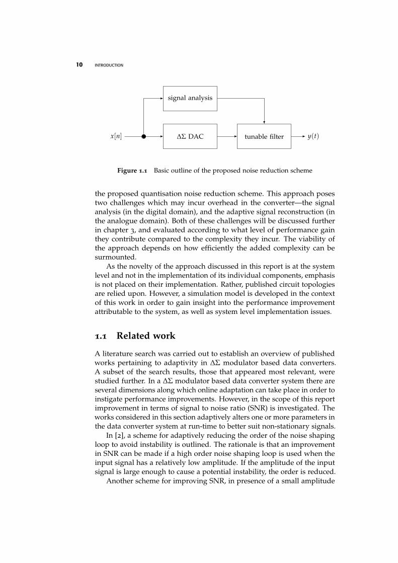
This thesis aims to explore whether it is feasible to dynamically alterthe bandwidth of the ∆Σ DAC in order to enhance the overall performance.To achieve this, the input signal must be analysed to obtain frequencydomain information, and this information must in turn be used to pro-gram the reconstruction filter with an appropriate transfer function. Thereconstructed bandwidth will be dynamic with respect to properties of theinput signal, and only spectral bands that contain signal energy will bereconstructed. Figure 1.1 on the following page shows a basic outline of

10 INTRODUCTION

x[n] ∆Σ DAC tunable filter

signal analysis

y(t)

Figure 1.1 Basic outline of the proposed noise reduction scheme

the proposed quantisation noise reduction scheme. This approach posestwo challenges which may incur overhead in the converter—the signalanalysis (in the digital domain), and the adaptive signal reconstruction (inthe analogue domain). Both of these challenges will be discussed furtherin chapter 3, and evaluated according to what level of performance gainthey contribute compared to the complexity they incur. The viability ofthe approach depends on how efficiently the added complexity can besurmounted.

As the novelty of the approach discussed in this report is at the systemlevel and not in the implementation of its individual components, emphasisis not placed on their implementation. Rather, published circuit topologiesare relied upon. However, a simulation model is developed in the contextof this work in order to gain insight into the performance improvementattributable to the system, as well as system level implementation issues.

1.1 Related work

A literature search was carried out to establish an overview of publishedworks pertaining to adaptivity in ∆Σ modulator based data converters.A subset of the search results, those that appeared most relevant, werestudied further. In a ∆Σ modulator based data converter system there areseveral dimensions along which online adaptation can take place in order toinstigate performance improvements. However, in the scope of this reportimprovement in terms of signal to noise ratio (SNR) is investigated. Theworks considered in this section adaptively alters one or more parameters inthe data converter system at run-time to better suit non-stationary signals.

In [2], a scheme for adaptively reducing the order of the noise shapingloop to avoid instability is outlined. The rationale is that an improvementin SNR can be made if a high order noise shaping loop is used when theinput signal has a relatively low amplitude. If the amplitude of the inputsignal is large enough to cause a potential instability, the order is reduced.

Another scheme for improving SNR, in presence of a small amplitude

INTRODUCTION 11

input signal, is presented in [3]. By amplifying weak input signals, theSNR is improved provided that the feedback signal in the ∆Σ modulatoris compensated accordingly. The signal strength can be sensed directlyat the input of the converter or by estimating the input signal strengthfrom the ∆Σ modulator output. An adaptation algorithm is used to selectappropriate gain for the pre-amplifier and for the feedback signal. Similarapproaches are reported in [4] and [5].

As will be further discussed in the next chapter (cf. page 21), a randomdither signal is frequently applied to the noise shaping loop of a ∆Σmodulator in order to avoid tonal noise components in the output signal.By applying the dither, the quantisation noise is made more white, resultingin a decorrelation of tonality. An inevitable side effect of this processis an increase in the noise floor, hence a reduced SNR performance ofthe converter. A dither capable of removing all tonal noise componentsmay result in an unacceptable decrease in SNR. The author of [6] hasmade the observation that tonal behaviour is most prominent when theamplitude of the input signal is small, and suggests adapting the dithersignal accordingly. The dither is modulated by the magnitude of the inputsignal so that full dither is applied when the instantaneous input signal isnear DC, and no dither is applied when the input signal is at full dynamicrange. Thereby a reduction in SNR performance is avoided when the ditheris not needed.

The aforementioned adaptation schemes all adapt the converter systembased on time domain properties of the input signal, or to some extent basedon statistical measures on the time series. The authors of [7] describe adigital synthesiser capable of frequency, phase, and quadrature modulation.The synthesiser uses a programmable bandpass ∆Σ modulator and adjuststhe notch frequency of the noise shaping function to suit the synthesisedsignal.

After studying available literature, it is apparent that dynamic run-timeadaptation of parameters in a ∆Σ modulator based data converter system,based on frequency domain properties of the input signal, is not previouslyreported.

1.2 Thesis outline

The remainder of this report is structured as follows: Chapter 2 providesbackground on relevant topics. In chapter 3, the proposed approach isdiscussed. In chapter 4, a simulation model is devised. The system issimulated and results are presented. Finally, in chapter 5, a conclusionregarding the viability of this approach is given along with an outlook tofurther work.

This page is intentionally left blank

background 2

This chapter provides background on topics relevant to the remainderof this report. The sections are structured according to figure 1.1 of theintroduction. First, the lowpass oversampling ∆Σ modulator based digitalto analogue converter (∆Σ DAC) is explained in more detail. Then, suitablearchitectures for the tunable filter will be explored, and finally, suitablemethods for signal analysis are considered.

2.1 Lowpass oversampling ∆Σ digital to analogue con-version

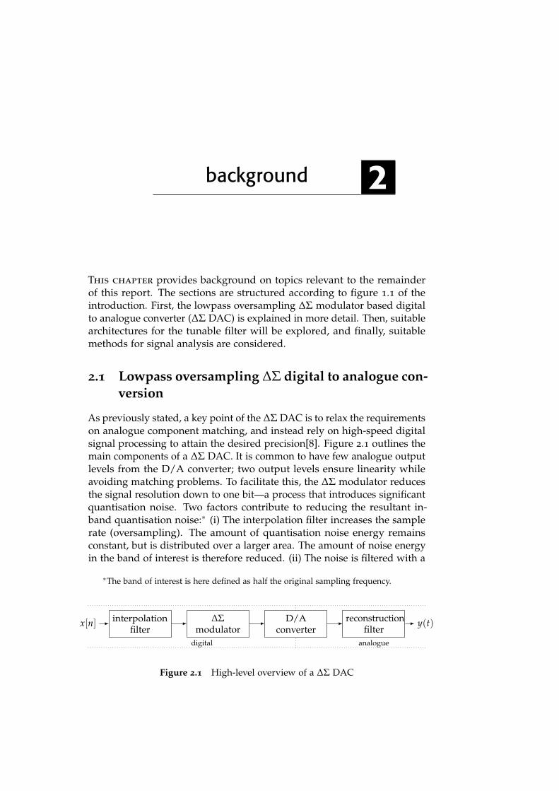
As previously stated, a key point of the ∆Σ DAC is to relax the requirementson analogue component matching, and instead rely on high-speed digitalsignal processing to attain the desired precision[8]. Figure 2.1 outlines themain components of a ∆Σ DAC. It is common to have few analogue outputlevels from the D/A converter; two output levels ensure linearity whileavoiding matching problems. To facilitate this, the ∆Σ modulator reducesthe signal resolution down to one bit—a process that introduces significantquantisation noise. Two factors contribute to reducing the resultant in-band quantisation noise:∗ (i) The interpolation filter increases the samplerate (oversampling). The amount of quantisation noise energy remainsconstant, but is distributed over a larger area. The amount of noise energyin the band of interest is therefore reduced. (ii) The noise is filtered with a

∗The band of interest is here defined as half the original sampling frequency.

x[n] interpolationfilter

∆Σmodulator

D/Aconverter

reconstructionfilter

y(t)

digital analogue

Figure 2.1 High-level overview of a ∆Σ DAC

14 BACKGROUND

x[n] ↑ N H(z) x[n]

Figure 2.2 Interpolation filter

highpass filter, while the signal remains unchanged (noise shaping). Thenoise is thus molded away from the band of interest. After reconstructingthe analogue output signal, only the band of interest remains. Hence, mostof the undesired spectral components are rejected.

In the following subsections, the workings of each module in the the∆Σ DAC will be discussed further. Finally, ideal estimates for noise perfor-mance are given.

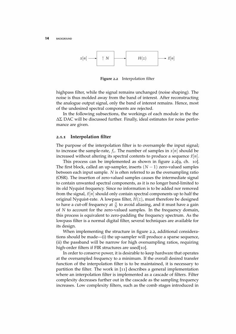
2.1.1 Interpolation filter

The purpose of the interpolation filter is to oversample the input signal;to increase the sample-rate, fs. The number of samples in x[n] should beincreased without altering its spectral contents to produce a sequence x[n].

This process can be implemented as shown in figure 2.2[9, ch. 10].The first block, called an up-sampler, inserts (N − 1) zero-valued samplesbetween each input sample. N is often referred to as the oversampling ratio(OSR). The insertion of zero-valued samples causes the intermediate signalto contain unwanted spectral components, as it is no longer band-limited toits old Nyquist frequency. Since no information is to be added nor removedfrom the signal, x[n] should only contain spectral components up to half theoriginal Nyquist-rate. A lowpass filter, H(z), must therefore be designedto have a cut-off frequency at π

N to avoid aliasing, and it must have a gainof N to account for the zero-valued samples. In the frequency domain,this process is equivalent to zero-padding the frequency spectrum. As thelowpass filter is a normal digital filter, several techniques are available forits design.

When implementing the structure in figure 2.2, additional considera-tions should be made—(i) the up-sampler will produce a sparse sequence,(ii) the passband will be narrow for high oversampling ratios, requiringhigh-order filters if FIR structures are used[10].

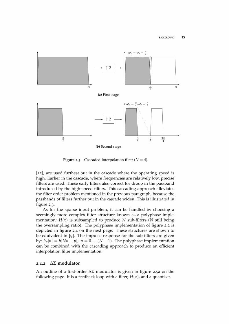
In order to conserve power, it is desirable to keep hardware that operatesat the oversampled frequency to a minimum. If the overall desired transferfunction of the interpolation filter is to be maintained, it is necessary topartition the filter. The work in [11] describes a general implementationwhere an interpolation filter is implemented as a cascade of filters. Filtercomplexity decreases further out in the cascade as the sampling frequencyincreases. Low complexity filters, such as the comb stages introduced in

BACKGROUND 15

↑ 2

π π2

π

ωp = ωs = π2

(a) First stage

↑ 2

π2

π4

3π4

ωp = π4 , ωs = π

2

π2

(b) Second stage

Figure 2.3 Cascaded interpolation filter (N = 4)

[12], are used furthest out in the cascade where the operating speed ishigh. Earlier in the cascade, where frequencies are relatively low, precisefilters are used. These early filters also correct for droop in the passbandintroduced by the high-speed filters. This cascading approach alleviatesthe filter order problem mentioned in the previous paragraph, because thepassbands of filters further out in the cascade widen. This is illustrated infigure 2.3.

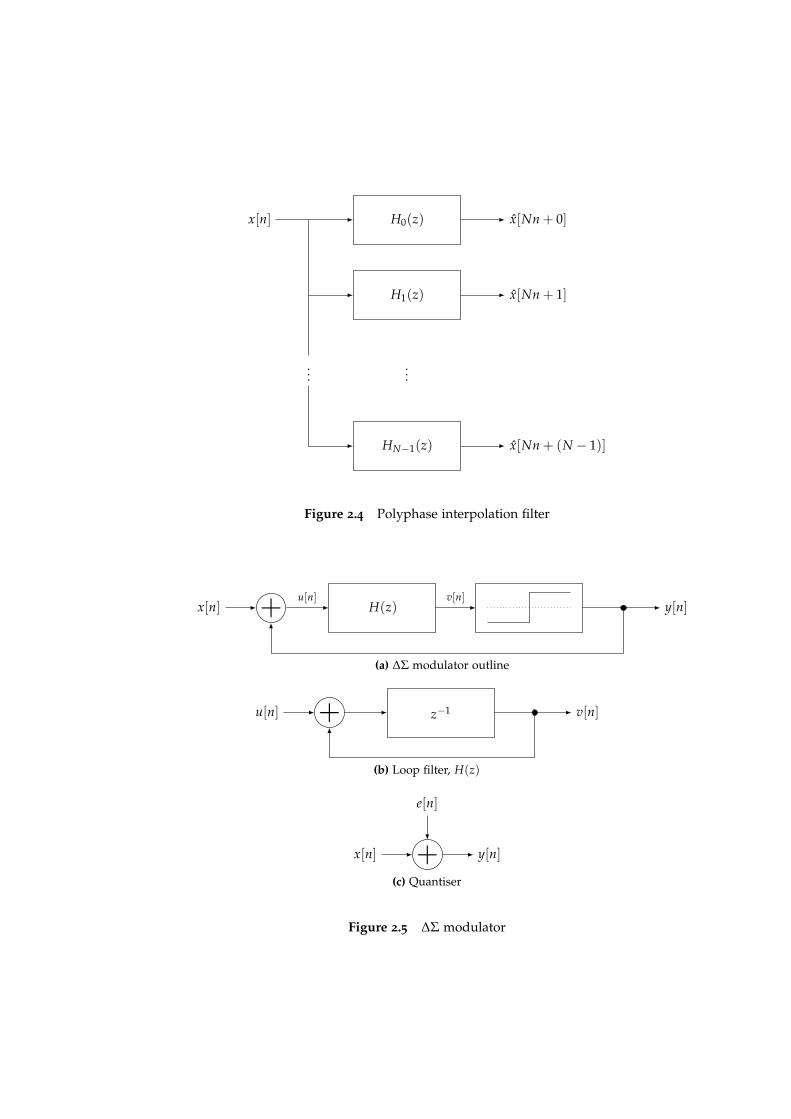
As for the sparse input problem, it can be handled by choosing aseemingly more complex filter structure known as a polyphase imple-mentation; H(z) is subsampled to produce N sub-filters (N still beingthe oversampling ratio). The polyphase implementation of figure 2.2 isdepicted in figure 2.4 on the next page. These structures are shown tobe equivalent in [9]. The impulse response for the sub-filters are givenby: hp[n] = h[Nn + p], p = 0 . . . (N − 1). The polyphase implementationcan be combined with the cascading approach to produce an efficientinterpolation filter implementation.

2.1.2 ∆Σ modulator

An outline of a first-order ∆Σ modulator is given in figure 2.5a on thefollowing page. It is a feedback loop with a filter, H(z), and a quantiser.

x[n] H0(z)

H1(z)

......

HN−1(z)

x[Nn + 0]

x[Nn + 1]

x[Nn + (N − 1)]

Figure 2.4 Polyphase interpolation filter

x[n] + H(z) y[n]u[n] v[n]

(a) ∆Σ modulator outline

u[n] + z−1 v[n]

(b) Loop filter, H(z)

x[n] + y[n]

e[n]

(c) Quantiser

Figure 2.5 ∆Σ modulator

BACKGROUND 17

The ∆Σ modulator reduces the input signal resolution to facilitate theactual D/A conversion. This process is called quantisation—the quantisermaps several input values to each output value. The difference between theoriginal and the quantised signal is called quantisation noise—a distortionintroduced by the quantiser. The quantiser can be modelled as simplyadding quantisation noise, e[n], to the input signal. This is depicted infigure 2.5c.

e[n] = y[n]− v[n] (2.1)

As the quantised signal contains less information, fewer bits are needed torepresent it. When quantising a high resolution input signal down to twolevels per sample (one bit), the quantisation noise can become excessive.

Oversampling contributes to reducing this noise, but it is often notpractical to oversample enough to obtain the desired precision. Therefore,to reduce the quantisation noise further, the ∆Σ modulator shapes the noiseaway from the band of interest.

Noise shaping

As is evident from figure 2.5 on the preceding page, H(z) acts on boththe input signal, x[n], and the quantisation error, e[n]. The system can bedescribed in the z-domain as follows:

Y(z) = X(z)H(z)

H(z) + 1+ E(z)

1H(z) + 1

(2.2)

From this, two transfer functions can be defined—a signal transfer function,S(z), and a noise transfer function, N(z).

S(z) =Y(z)X(z)

=H(z)

H(z) + 1(2.3)

N(z) =Y(z)E(z)

=1

H(z) + 1(2.4)

In a lowpass ∆Σ DAC, it is usually suitable to shift the quantisation noiseto high frequencies, away from the band of interest. If H(z) is defined as:

H(z) =1

z − 1(2.5)

S(z) and N(z) becomes:S(z) = z−1 (2.6)

N(z) = 1 − z−1 (2.7)

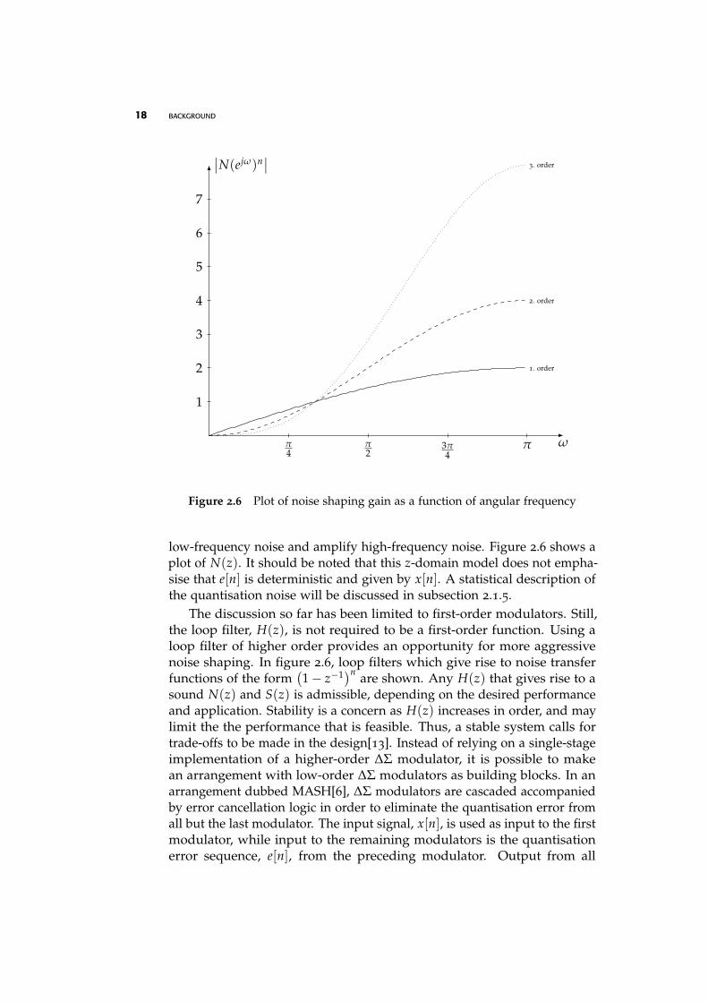
S(z) is simply a delay and does not alter the frequency spectrum, whileN(z) has a highpass frequency characteristic. N(z) will therefore suppress

18 BACKGROUND

1. order

2. order

3. order

ω

∣∣N(ejω)n∣∣

1

2

3

4

5

6

7

π4

π2

3π4

π

Figure 2.6 Plot of noise shaping gain as a function of angular frequency

low-frequency noise and amplify high-frequency noise. Figure 2.6 shows aplot of N(z). It should be noted that this z-domain model does not empha-sise that e[n] is deterministic and given by x[n]. A statistical description ofthe quantisation noise will be discussed in subsection 2.1.5.

The discussion so far has been limited to first-order modulators. Still,the loop filter, H(z), is not required to be a first-order function. Using aloop filter of higher order provides an opportunity for more aggressivenoise shaping. In figure 2.6, loop filters which give rise to noise transferfunctions of the form

(1 − z−1)n are shown. Any H(z) that gives rise to a

sound N(z) and S(z) is admissible, depending on the desired performanceand application. Stability is a concern as H(z) increases in order, and maylimit the the performance that is feasible. Thus, a stable system calls fortrade-offs to be made in the design[13]. Instead of relying on a single-stageimplementation of a higher-order ∆Σ modulator, it is possible to makean arrangement with low-order ∆Σ modulators as building blocks. In anarrangement dubbed MASH[6], ∆Σ modulators are cascaded accompaniedby error cancellation logic in order to eliminate the quantisation error fromall but the last modulator. The input signal, x[n], is used as input to the firstmodulator, while input to the remaining modulators is the quantisationerror sequence, e[n], from the preceding modulator. Output from all

BACKGROUND 19

modulators is used as input to the error cancellation logic which forms theoutput, y[n]. Unfortunately, the output from the MASH arrangement isinherently multibit, and thus incurs an increased complexity in the D/Amodule—either by requiring preprocessing of the multibit signal or byrequiring several analogue output levels.

In summary, the ∆Σ modulator produces a single-bit representationof the input where most of the truncation error is contained in the high-frequency portion of the spectrum. The ∆Σ modulator does this by quan-tising the input signal, while shaping the resultant quantisation noise.

2.1.3 D/A conversion

The D/A converter is the interface between the digital and analogue do-mains. It takes as input a sequence of bits from the ∆Σ modulator andproduces a corresponding output sequence of sampled analogue values.These analogue samples are represented by some physical quantity, suchas a voltage potential or an electric current.

When the ∆Σ DAC is using a two-level quantiser, the D/A conversionis inherently linear. The spacing between the output levels does not matter,as long as the levels are stable. Several second-order effects may, however,corrupt the ideal linearity—power supply noise will make the output levelsfluctuate, perhaps to a noticeable extent. Over-shoot and under-shoot, andrise-time and fall-time, may introduce distortion at the output, dependingon the choice of reconstruction filter (cf. section 2.2 on page 22).

2.1.4 Reconstruction filter

The oversampled portion of the frequency spectrum is used by the ∆Σ DACto hold quantisation noise. As discussed in subsection 2.1.2, a significantamount of quantisation noise is shifted from the band of interest into theoversampled spectrum. At the output of the ∆Σ DAC, the analogue signalis reconstructed by band limiting it to a frequency, fb, the band of interest.For many applications this would be about half the original samplingfrequency.

The reconstruction filter takes as input the sequence of analogue sam-ples from the D/A converter, and outputs a continuous time signal, y(t).The reconstruction filter may consist of several stages. Implementation al-ternatives for the reconstruction filter which are suitable for this applicationare discussed in section 2.2 on page 22.

2.1.5 Performance

The purpose of this subsection is to estimate the performance of a ∆Σ DACin terms of signal to noise ratio (SNR).

20 BACKGROUND

When analysing the noise performance of the ∆Σ DAC, the non-linearbehaviour of the quantiser presents a challenge. It is common to simplifythe analysis by assuming the input, x[n], to be busy and therefore seem-ingly uncorrelated with the quantisation noise, e[n]. In statistical terms,e[n] is modelled as a zero-mean white noise wide-sense stationary (WSS)process. This enables linear analysis and simplifies estimating the powerspectrum[14, 15, 16]. Furthermore, the quantiser is assumed to be uniform∗

with two output levels (one bit) and the ∆Σ DAC input to be a signedinteger, b bits long. Using these assumptions, it is possible to quantify theworst-case quantisation error as:

− emax ≤ e[n] ≤ emax, emax = 2b−1 − 1 (2.8)

The absolute value of e[n], for all n, is limited to a quantity emax. It isimplied, from the assumptions above, that each of the possible values areequally likely.

For a zero-mean white-noise process, the power spectrum is equal tothe variance of the process[17].

Pe(ejω) = σ2e = E{e2} ∝

12emax + 1

emax

∑k=−emax

k2 =4b − 2b+1

12(2.9)

Pe is independent of ω and independent of the sampling frequency, fs,so the amount of quantisation noise introduced by the ∆Σ modulator isconstant and defined by b, the number of bits in the input word.

Quantisation noise undergoes noise shaping in the digital domain asdiscussed in subsection 2.1.2 on page 15. The resulting noise shaped powerspectrum, Pe,ns, can be expressed as:

Pe,ns(ejω) = σ2e

∣∣∣N(ejω)∣∣∣2

= σ2e

(1 − e−jω

) (1 − ejω

)(2.10)

= 2σ2e (cos ω − 1) (2.11)

In the digital domain, the frequency variable is normalised such that2π corresponds to fs. When going from the digital to the analogue domain,the digital frequency variable ω is mapped to an analogue frequency f :

ω =2π f

fs(2.12)

It must also be taken into account that only the band of interest, fb, willpass through the analogue reconstruction filter, R(s). For the purpose ofestimating SNR performance, R(s) is assumed to be an ideal brick-wall

∗A uniform quantiser rounds an input sample to the closest output level

BACKGROUND 21

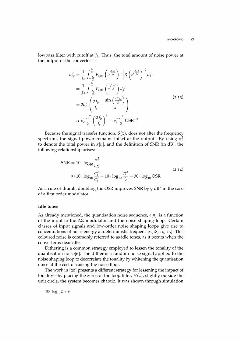
lowpass filter with cutoff at fb. Thus, the total amount of noise power atthe output of the converter is:

σ2ey =

1fs

∫ fs2

− fs2

Pe,ns

(ej 2π f

fs

)·∣∣∣∣R (

ej 2π ffs

)∣∣∣∣2

d f

=1fs

∫ fb2

− fb2

Pe,ns

(ej 2π f

fs

)d f

= 2σ2e

2 fb

fs−

sin(

2π fbfs

)π

≈ σ2

eπ2

3

(2 fb

fs

)3

= σ2e

π2

3OSR−3

(2.13)

Because the signal transfer function, S(z), does not alter the frequencyspectrum, the signal power remains intact at the output. By using σ2

xto denote the total power in x[n], and the definition of SNR (in dB), thefollowing relationship arises:

SNR = 10 · log10σ2

xσ2

ey

≈ 10 · log10σ2

xσ2

e− 10 · log10

π2

3+ 30 · log10 OSR

(2.14)

As a rule of thumb, doubling the OSR improves SNR by 9 dB∗ in the caseof a first order modulator.

Idle tones

As already mentioned, the quantisation noise sequence, e[n], is a functionof the input to the ∆Σ modulator and the noise shaping loop. Certainclasses of input signals and low-order noise shaping loops give rise toconcentrations of noise energy at deterministic frequencies[18, 19, 15]. Thiscoloured noise is commonly referred to as idle tones, as it occurs when theconverter is near idle.

Dithering is a common strategy employed to lessen the tonality of thequantisation noise[6]. The dither is a random noise signal applied to thenoise shaping loop to decorrelate the tonality by whitening the quantisationnoise at the cost of raising the noise floor.

The work in [20] presents a different strategy for lessening the impact oftonality—by placing the zeros of the loop filter, H(z), slightly outside theunit circle, the system becomes chaotic. It was shown through simulation

∗30 · log10 2 ≈ 9

22 BACKGROUND

that tonality is reduced. As with dithering, this approach raises the noisefloor. The study reported in [21] concludes that chaos is less efficient thandithering.

2.2 Tunable filter

In a ∆Σ DAC, the purpose of the reconstruction filter is to reject theoversampled portion of the spectrum and only pass through the band ofinterest. In a lowpass ∆Σ DAC, this amounts to lowpass filtering the D/Aconverted ∆Σ bitstream. While it is possible to use any kind of analoguefilter topology, sampled data filters are usually preferred. Like digital filters,sampled data filters process sampled input signals. However, the samplesare not quantised, and they are stored as a physical quantity, usually acharge or a current, hence the precision of the samples are only limitedby the performance of the signal processing components. When usingsampled data techniques, it is thus possible to relax the requirements on theswitching characteristics of the D/A converter compared to a continuoustime filter, and to avoid the need for return-to-zero (RTZ) or similar outputcoding.

In this report, only switched-capacitor based filters, where samplesare stored as charges in capacitors, are considered. Switched-currentfilters, where samples are stored as currents, have some salient features,but reported switched-capacitor structures are still able to attain higherperformance in terms of accuracy and noise[22]. In the following subsection,the basic principles of switched-capacitor integrators are discussed. Becausethe scheme outlined in chapter 1 requires a tunable filter, structures withtunable transfer functions are needed. This is discussed in subsection 2.2.3on page 25.

2.2.1 Switched-capacitor basics

Switched-capacitor refers to a technique for implementing resistor ap-proximations using switches and capacitors. Switches can in turn beimplemented using transistors, and thus, the technique lends itself wellfor use in integrated circuits when a large resistance is required. Theswitched-capacitor resistor approximations are commonly found in fil-tering applications, but are also used in, for example, gain stages andoscillators[23].

Figure 2.7 on the facing page shows a simplified switched-capacitorresistor approximation. Here, φ1 and φ2 are two non-overlapping phasesof a clock signal controlling the switches S1 and S2. The length of a clockcycle is denoted T, thus, φ1 and φ2 are each active slightly less than T/2every clock cycle. The nodes V1 and V2 are connected to voltage sources

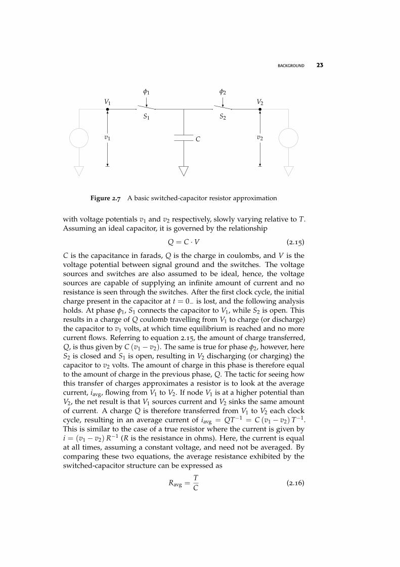
BACKGROUND 23

V1

C

V2

S1 S2

φ1 φ2

v1 v2

Figure 2.7 A basic switched-capacitor resistor approximation

with voltage potentials v1 and v2 respectively, slowly varying relative to T.Assuming an ideal capacitor, it is governed by the relationship

Q = C · V (2.15)

C is the capacitance in farads, Q is the charge in coulombs, and V is thevoltage potential between signal ground and the switches. The voltagesources and switches are also assumed to be ideal, hence, the voltagesources are capable of supplying an infinite amount of current and noresistance is seen through the switches. After the first clock cycle, the initialcharge present in the capacitor at t = 0− is lost, and the following analysisholds. At phase φ1, S1 connects the capacitor to V1, while S2 is open. Thisresults in a charge of Q coulomb travelling from V1 to charge (or discharge)the capacitor to v1 volts, at which time equilibrium is reached and no morecurrent flows. Referring to equation 2.15, the amount of charge transferred,Q, is thus given by C (v1 − v2). The same is true for phase φ2, however, hereS2 is closed and S1 is open, resulting in V2 discharging (or charging) thecapacitor to v2 volts. The amount of charge in this phase is therefore equalto the amount of charge in the previous phase, Q. The tactic for seeing howthis transfer of charges approximates a resistor is to look at the averagecurrent, iavg, flowing from V1 to V2. If node V1 is at a higher potential thanV2, the net result is that V1 sources current and V2 sinks the same amountof current. A charge Q is therefore transferred from V1 to V2 each clockcycle, resulting in an average current of iavg = QT−1 = C (v1 − v2) T−1.This is similar to the case of a true resistor where the current is given byi = (v1 − v2) R−1 (R is the resistance in ohms). Here, the current is equalat all times, assuming a constant voltage, and need not be averaged. Bycomparing these two equations, the average resistance exhibited by theswitched-capacitor structure can be expressed as

Ravg =TC

(2.16)

24 BACKGROUND

In practical switched-capacitor circuits, none of the components makingup the approximated resistor will be ideal. These non-idealities contributeto distortion and noise; some more than others. As the switches are usuallyimplemented by MOSFET transistors, they will exhibit a finite non-zeroresistance, Ron, when conducting. This resistance must be small enough sothat the time constant formed by it and the capacitor leaves enough timefor settling. The transistors used in the switches will release their channelcharge when turned off. This signal dependent charge will contribute tothe charge already stored in the capacitor and cause a voltage offset. Theclock signals can therefore be said to feed through into the signal path∗.The switches will also contribute thermal and 1/ f noise, as well as junctionleakage current. In many common configurations, the switch-capacitoris driven by an operational amplifier (op-amp) approximating a voltagesource. The switched-capacitor circuit will therefore suffer a degradation inperformance due to imperfections of the op-amp. Common non-idealitiesthat need attention in switched-capacitor circuit design include offset volt-age, gain bandwidth (GBW), slew rate, output resistance, and thermal and1/ f noise.

Various circuit implementation techniques are available for improvingthe performance of switched-capacitor circuits[24], including chopper mod-ulation, which is used to escape 1/ f noise as the input signal is modulatedto a higher frequency before amplification, and demodulated afterwards.Correlated double sampling (CDS) is often used to compensate for voltageoffset and finite gain in the op-amp, whereby low frequency noise andop-amp offset is sampled and then subtracted.

2.2.2 Switched-capacitor filter structures

As switched-capacitor based filters are operating in the z-domain, both FIRand IIR realisations are possible.

A switched-capacitor filter IIR structure can be obtained by simplyreplacing resistors with switched-capacitor resistor approximations in acontinuous time prototype. Another strategy is to factor the transfer func-tion into a cascade of second-order sections, and use specialised switched-capacitor biquads for their realisation. The final structure will then benefitfrom a performance gain inherited from the building blocks, as these areoften tuned to work around switched-capacitor non-idealities.

As the absolute equivalent resistance of the switched-capacitor resistorapproximation is only dependent on the clocking frequency and the capaci-tance value, accurate transfer functions can be realised as the accuracy ofthe poles and zeros depends on the ratios between capacitors, and not on

∗If a manufacturing process without self-aligned gates is used, the clock will also becapacitively coupled to the source and drain of transistors because of overlap

BACKGROUND 25

absolute matching between capacitors and resistors. Even though preciseabsolute capacitance values can be difficult to achieve in integrated circuits,matching between capacitor devices in a monolithic circuit can be madevery accurate if careful layout principles are adhered to[25]. The manu-factured level of accuracy may be sufficient for many applications, thusavoiding the need for post-fabrication trimming.

It may be necessary to reduce the sampling rate prior to reconstructingthe output signal if important criterions, such as power constraints, cannotbe met at the oversampled output rate. Several switched-capacitor baseddecimation structures are reported[26, 27, 28].

2.2.3 Tunable switched-capacitor filters

The convenient tunability of switched-capacitor filters stems from thetunability of the resistance exhibited by the switched-capacitor resistorapproximations. As already stated, the equivalent resistance is given bythe capacitance value and the clock frequency. Thus, by altering the clockfrequency or the capacitance value, the equivalent resistance changes. Theclock frequency can be down-converted in the digital domain by a frequencydivider. If it is not practical to alter the clock frequency, the capacitor canbe replaced by a programmable capacitor array. Each capacitor in thecapacitor array can be programmed to be grounded or left floating. Thus,the capacitance exhibited by the array will depend on which capacitorsare active. In [29], a lowpass switched-capacitor filter with three selectablecutoff frequencies is presented. Programmability is achieved by digitallyswitching capacitors in or out.

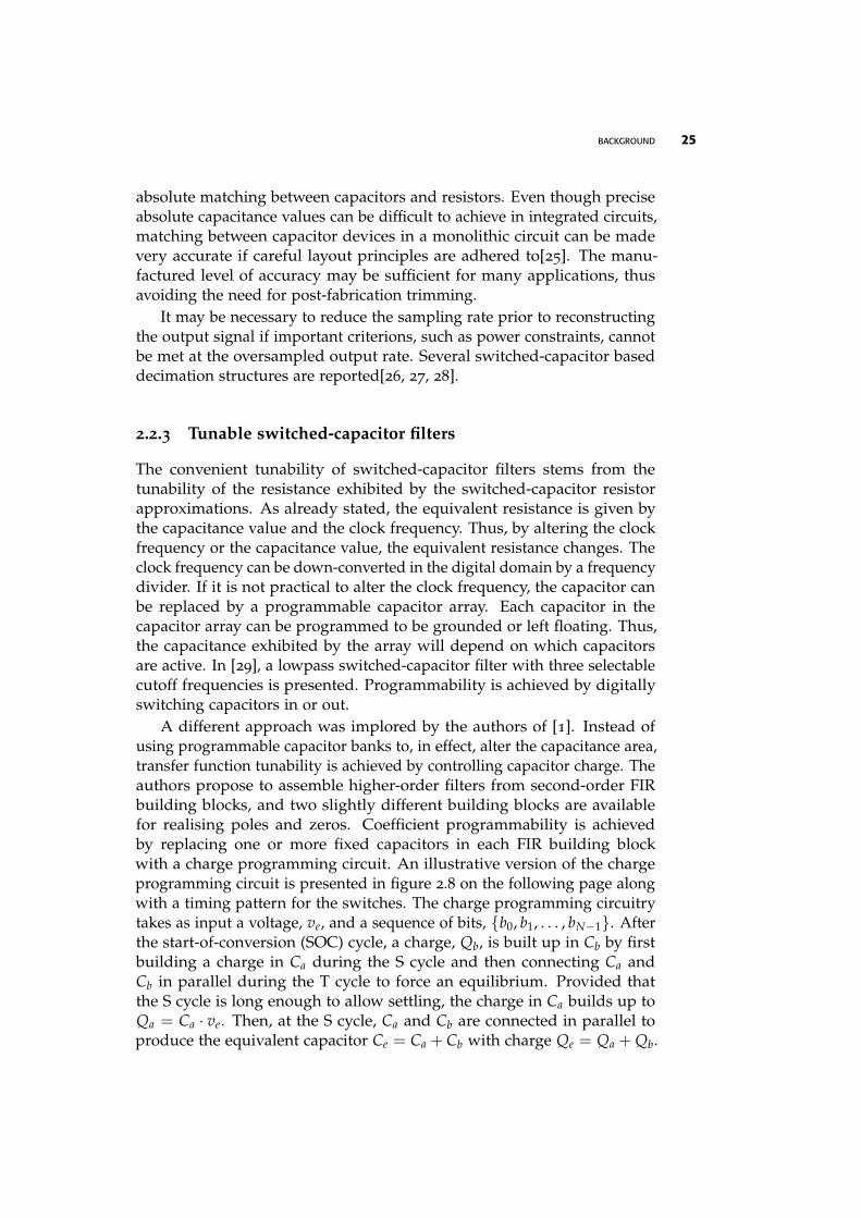
A different approach was implored by the authors of [1]. Instead ofusing programmable capacitor banks to, in effect, alter the capacitance area,transfer function tunability is achieved by controlling capacitor charge. Theauthors propose to assemble higher-order filters from second-order FIRbuilding blocks, and two slightly different building blocks are availablefor realising poles and zeros. Coefficient programmability is achievedby replacing one or more fixed capacitors in each FIR building blockwith a charge programming circuit. An illustrative version of the chargeprogramming circuit is presented in figure 2.8 on the following page alongwith a timing pattern for the switches. The charge programming circuitrytakes as input a voltage, ve, and a sequence of bits, {b0, b1, . . . , bN−1}. Afterthe start-of-conversion (SOC) cycle, a charge, Qb, is built up in Cb by firstbuilding a charge in Ca during the S cycle and then connecting Ca andCb in parallel during the T cycle to force an equilibrium. Provided thatthe S cycle is long enough to allow settling, the charge in Ca builds up toQa = Ca · ve. Then, at the S cycle, Ca and Cb are connected in parallel toproduce the equivalent capacitor Ce = Ca + Cb with charge Qe = Qa + Qb.

26 BACKGROUND

vs

−Cc

+

eoc

Cb

so

c

t

Ca

s·bi

s · bi

ve

(a) schematic

soc

· · ·

eoc

· · ·

s

· · ·

t

· · ·

b0 b1 bN−1· · ·

(b) timing pattern

Figure 2.8 The charge programming circuit from [1]

Assuming Ca = Cb, the following relationship arise:

vn = ve

n

∑i=0

2i−n−1bi (2.17)

Where vn is the voltage drop over Ce after input bit bn. The output, vs,is driven by an op-amp in an inverting integrator configuration. At theend-of-conversion (EOC) cycle, the open loop gain of the op-amp willdrive Cb towards a short circuit between the true ground and the virtualground at the negative input terminal of the op-amp, forcing the capacitorto release its charge, Qb, to be subsequently trapped by Cc in the invertingintegrator configuration and resulting in:

vs = −Qb

Cc= −vn

Cb

Cc, n = N − 1

= −veCb

Cc

N−1

∑i=0

2i−N−2bi

(2.18)

The authors present circuit level simulations of a filter built from the FIRbuilding blocks. The filter uses one FIR building block for poles and fourFIR building blocks for zeroes, arriving at 8 zeroes and 2 poles, and iscapable of filter coefficient programmability with a resolution of 8 bits.The circuit simulations demonstrate a good agreement between ideal andsimulated frequency response.

BACKGROUND 27

2.3 Signal analysis

In the context of this work, the purpose of the signal analysis is to extractproperties from the input signal in order to obtain programming informa-tion for the output signal reconstruction filter. This amounts to findingthe spectral contents of the input signal, x[n], as a function of time. In thissection, background for the signal analysis is presented. Signal analysis inthe context of this work is discussed further in section 3.1.1 on page 33.

2.3.1 The short time Fourier transform

The Fourier transform provides a frequency domain description of a signaland is a widely used and established method for signal analysis[30, 31].

An N-length sequence of samples, x[n], can be expressed in terms of itstransfer domain coefficients[9, ch. 3], X[k], as:

x[n] =1N

N−1

∑k=0

X[k]ej2πkn

N , 0 ≤ n ≤ N − 1 (2.19)

Where

X[k] =N−1

∑k=0

x[n]e−j2πkn

N , 0 ≤ k ≤ N − 1 (2.20)

Equation 2.20 is usually referred to as the discrete Fourier transform(DFT), while 2.19 is referred to as the inverse discrete Fourier transform(IDFT). These transforms are usually implemented using efficient algo-rithms known as the fast Fourier transform (FFT) and the inverse fastFourier transform (IFFT)[32].

The squared magnitude of the transform coefficients, |X[k]|2, revealshow much power each frequency component contributes. However, theyleave no reference to when they are occuring. In the context of this work,the spectral contents of the input needs to be tracked over time. Theremainder of this subsection discusses the short time Fourier transform(STFT), which provides positioning in time for the transform coefficients.The localisation in time provided by the STFT is achieved by windowingthe input signal. The window extracts a portion of the signal in time, thus,the frequency components reported by the transform must be occurringinside the window. The STFT results in a three-dimensional data set thatcan be visualised as a spectrogram plot. A common configuration is to usetime as the x-axis, frequency as the y-axis, and power as a colour intensity,the z-axis.

The window used in the transform can be described in the time domainby its weights. Each weight is multiplied by its corresponding sample.The non-zero weights define which samples are to be extracted from the

28 BACKGROUND

sequence. By making the window narrower in the time dimension, the local-isation property improves because fewer samples are extracted. However,this also results in fewer transform coefficients, and hence, a more coarsefrequency resolution. This calls for an application-specific trade-off whendesigning the system. The DFT assumes a periodic function, with periodequal to the length of the sequence. Thus, clipping an arbitrary signal intime may introduce distortion, which corrupts the analysis. To lessen thedistortion, an artificial periodicity is introduced by choosing the weightsso that they attenuate the beginning and end of the extracted sequence. Inturn, this may require some overlap in the analysis to capture the entiresignal in the transform domain. From the weights, several important perfor-mance metrics can be inferred. The work in [33] provides a comprehensiveoverview of windows in general, along with performance metrics and acomparison. The work in [34] presents a method for generating customisedwindows that, e.g., can be tuned to be more sensitive to certain frequenciesas it provides the designer with some degrees of freedom.

2.3.2 Wavelets

The use of wavelet analysis and synthesis can be advantageous for certainapplications. The analysis wavelet, which in turn makes up the basis, haslocalisation in both time and frequency. This is an important property of thewavelet transform, and in contrast to Fourier analysis where the frequencycomponents are pure tones with an infinite extent in time—requiring theintroduction of artificial periodicity by means of windowing if localisationin time is required (cf. subsection 2.3.1 on the preceding page).

Wavelet analysis decomposes the input signal into a linear combinationof dilated and time shifted versions of the analysis wavelet, ψ(t)—forminga wavelet basis, ψkn(t), from the initial wavelet function. A signal, x(t),can be expressed in terms of its wavelet transform coefficients, ckn, and thewavelet basis as[35]:

x(t) = ∑k,n

cknψkn(t) (2.21)

whereψkn(t) = 2

k2 ψ

(2kt − n

)(2.22)

provided that x(t) and ψ(t) meet certain requirements. n represents thetime shift, while k defines the amount of dilation. ckn can be computed asthe inner product between x(t) and ψkn(t):

ckn = 〈x(t), ψkn(t)〉 (2.23)

Equations 2.21 and 2.23 are not the most general form of the wavelet trans-form, but a discrete version that dyadically samples the analysis wavelet.Equation 2.21 synthesises the signal, x(t), from its wavelet coefficients, ckn,

BACKGROUND 29

t

ψ(t)

(a) Analysis wavelet

n

hH [n]

−0.5

−0.3

−0.1

0.1

0.3

0.5

0.7

0 1 2 3 4 5

(b) Impulse response

Figure 2.9 The Daubechies wavelet with three vanishing moments

x[n]

HH(z)

HL(z)

HH(z)

HL(z) · · ·

HH(z)

HL(z)

stor

age

ortr

ans-

mis

sion

chan

nel

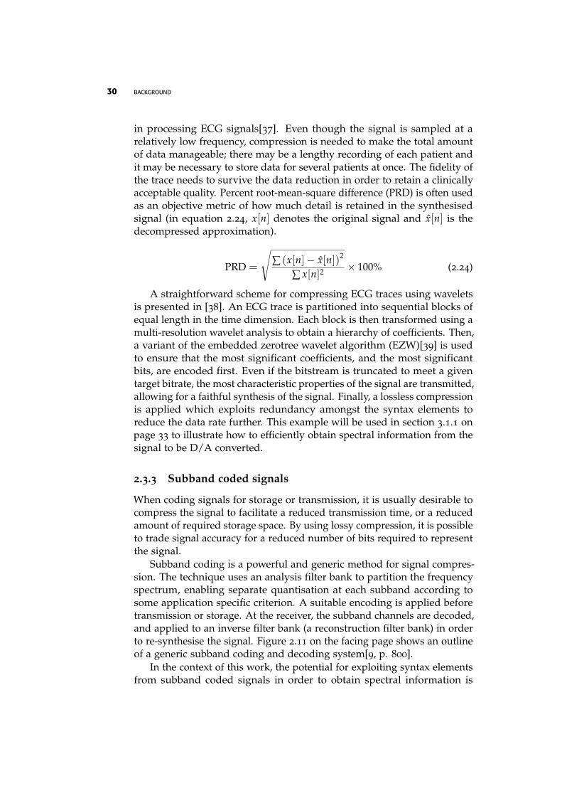
Figure 2.10 Wavelet analysis implemented by a filter bank

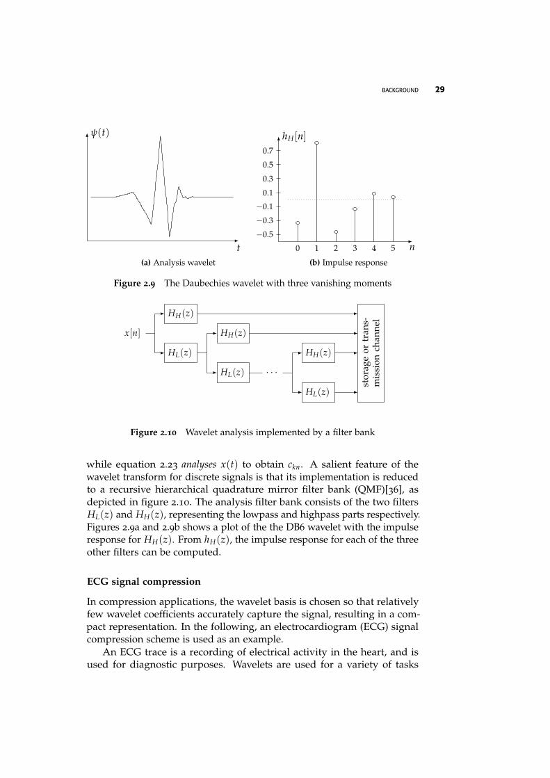
while equation 2.23 analyses x(t) to obtain ckn. A salient feature of thewavelet transform for discrete signals is that its implementation is reducedto a recursive hierarchical quadrature mirror filter bank (QMF)[36], asdepicted in figure 2.10. The analysis filter bank consists of the two filtersHL(z) and HH(z), representing the lowpass and highpass parts respectively.Figures 2.9a and 2.9b shows a plot of the the DB6 wavelet with the impulseresponse for HH(z). From hH(z), the impulse response for each of the threeother filters can be computed.

ECG signal compression

In compression applications, the wavelet basis is chosen so that relativelyfew wavelet coefficients accurately capture the signal, resulting in a com-pact representation. In the following, an electrocardiogram (ECG) signalcompression scheme is used as an example.

An ECG trace is a recording of electrical activity in the heart, and isused for diagnostic purposes. Wavelets are used for a variety of tasks

30 BACKGROUND

in processing ECG signals[37]. Even though the signal is sampled at arelatively low frequency, compression is needed to make the total amountof data manageable; there may be a lengthy recording of each patient andit may be necessary to store data for several patients at once. The fidelity ofthe trace needs to survive the data reduction in order to retain a clinicallyacceptable quality. Percent root-mean-square difference (PRD) is often usedas an objective metric of how much detail is retained in the synthesisedsignal (in equation 2.24, x[n] denotes the original signal and x[n] is thedecompressed approximation).

PRD =

√∑ (x[n]− x[n])2

∑ x[n]2× 100% (2.24)

A straightforward scheme for compressing ECG traces using waveletsis presented in [38]. An ECG trace is partitioned into sequential blocks ofequal length in the time dimension. Each block is then transformed using amulti-resolution wavelet analysis to obtain a hierarchy of coefficients. Then,a variant of the embedded zerotree wavelet algorithm (EZW)[39] is usedto ensure that the most significant coefficients, and the most significantbits, are encoded first. Even if the bitstream is truncated to meet a giventarget bitrate, the most characteristic properties of the signal are transmitted,allowing for a faithful synthesis of the signal. Finally, a lossless compressionis applied which exploits redundancy amongst the syntax elements toreduce the data rate further. This example will be used in section 3.1.1 onpage 33 to illustrate how to efficiently obtain spectral information from thesignal to be D/A converted.

2.3.3 Subband coded signals

When coding signals for storage or transmission, it is usually desirable tocompress the signal to facilitate a reduced transmission time, or a reducedamount of required storage space. By using lossy compression, it is possibleto trade signal accuracy for a reduced number of bits required to representthe signal.

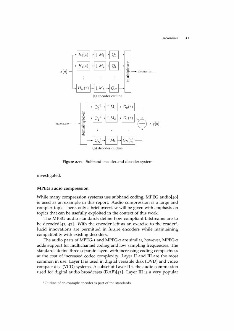
Subband coding is a powerful and generic method for signal compres-sion. The technique uses an analysis filter bank to partition the frequencyspectrum, enabling separate quantisation at each subband according tosome application specific criterion. A suitable encoding is applied beforetransmission or storage. At the receiver, the subband channels are decoded,and applied to an inverse filter bank (a reconstruction filter bank) in orderto re-synthesise the signal. Figure 2.11 on the facing page shows an outlineof a generic subband coding and decoding system[9, p. 800].

In the context of this work, the potential for exploiting syntax elementsfrom subband coded signals in order to obtain spectral information is

BACKGROUND 31

x[n]

H0(z)

H1(z)

...

HN(z)

↓ M1

↓ M2

...

↓ ML

Q0

Q1

...

QN

mu

ltip

lexe

r

01010110110 · · ·

(a) encoder outline

01010110110 · · ·

dem

ult

iple

xer

Q−10

Q−11

...

Q−1N

↑ M1

↑ M2

...

↑ ML

G0(z)

G1(z)

...

GN(z)

+ y[n]

(b) decoder outline

Figure 2.11 Subband encoder and decoder system

investigated.

MPEG audio compression

While many compression systems use subband coding, MPEG audio[40]is used as an example in this report. Audio compression is a large andcomplex topic—here, only a brief overview will be given with emphasis ontopics that can be usefully exploited in the context of this work.

The MPEG audio standards define how compliant bitstreams are tobe decoded[41, 42]. With the encoder left as an exercise to the reader∗,lucid innovations are permitted in future encoders while maintainingcompatibility with existing decoders.

The audio parts of MPEG-1 and MPEG-2 are similar, however, MPEG-2adds support for multichannel coding and low sampling frequencies. Thestandards define three separate layers with increasing coding compactnessat the cost of increased codec complexity. Layer II and III are the mostcommon in use. Layer II is used in digital versatile disk (DVD) and videocompact disc (VCD) systems. A subset of Layer II is the audio compressionused for digital audio broadcasts (DAB)[43]. Layer III is a very popular

∗Outline of an example encoder is part of the standards

32 BACKGROUND

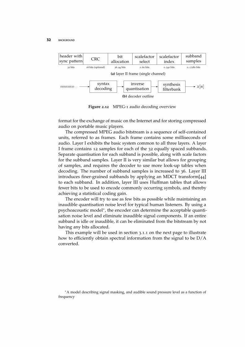
header withsync pattern CRC bit

allocationscalefactor

selectscalefactor

indexsubbandsamples

32 bits 16 bits (optional) 26..94 bits 0..60 bits 0..540 bits 0..17280 bits

(a) layer II frame (single channel)

01010110110 · · ·syntax

decodinginverse

quantisationsynthesisfilterbank

x[n]

(b) decoder outline

Figure 2.12 MPEG-1 audio decoding overview

format for the exchange of music on the Internet and for storing compressedaudio on portable music players.

The compressed MPEG audio bitstream is a sequence of self-containedunits, referred to as frames. Each frame contains some milliseconds ofaudio. Layer I exhibits the basic system common to all three layers. A layerI frame contains 12 samples for each of the 32 equally spaced subbands.Separate quantisation for each subband is possible, along with scale factorsfor the subband samples. Layer II is very similar but allows for groupingof samples, and requires the decoder to use more look-up tables whendecoding. The number of subband samples is increased to 36. Layer IIIintroduces finer-grained subbands by applying an MDCT transform[44]to each subband. In addition, layer III uses Huffman tables that allowsfewer bits to be used to encode commonly occurring symbols, and therebyachieving a statistical coding gain.

The encoder will try to use as few bits as possible while maintaining aninaudible quantisation noise level for typical human listeners. By using apsychoacoustic model∗, the encoder can determine the acceptable quanti-sation noise level and eliminate inaudible signal components. If an entiresubband is idle or inaudible, it can be eliminated from the bitstream by nothaving any bits allocated.

This example will be used in section 3.1.1 on the next page to illustratehow to efficiently obtain spectral information from the signal to be D/Aconverted.

∗A model describing signal masking, and audible sound pressure level as a function offrequency

theory 3

As stated in the introduction, the purpose of this report is to investigatewhether making the bandwidth of the ∆Σ DAC dynamic with respect toproperties of the input signal, yields a large enough performance gain tojustify the complexity it incurs. In this chapter, strategies for implementingthe building blocks of the system are discussed. Then, system level imple-mentation issues are considered, and estimates of the performance gainattributable to the system are given.

3.1 Implementation

The implementation of the signal analysis and the tunable reconstructionfilter needs to be as simple as possible in order to introduce the leastamount of overhead compared to a static converter. Less overhead givesbetter performance in terms of complexity; thus a more viable approach.

First, considerations are made with respect to implementing the signalanalysis circuitry, and how it can be simplified if the DAC is to some extentintegrated with a signal decompression system. Then, some architecturesfor the tunable reconstruction filter are discussed.

3.1.1 Signal analysis

The purpose of the signal analysis in this application is to reveal the spectralcontents of the input signal as a function of time. This information willin turn be used to tune the reconstruction filter so that only the spectralbands that contain energy will be reconstructed. The input to the analysistask is a digital signal, x[n], a replica of the input to the ∆Σ DAC. Theoutput is a list of digital control words for the tunable reconstruction filter.This process is conceptually depicted in figure 3.1 on the following page:Relevant properties are extracted from x[n], and then mapped into controlwords, c[n]. The purpose of the control word mapping is to provide a layer

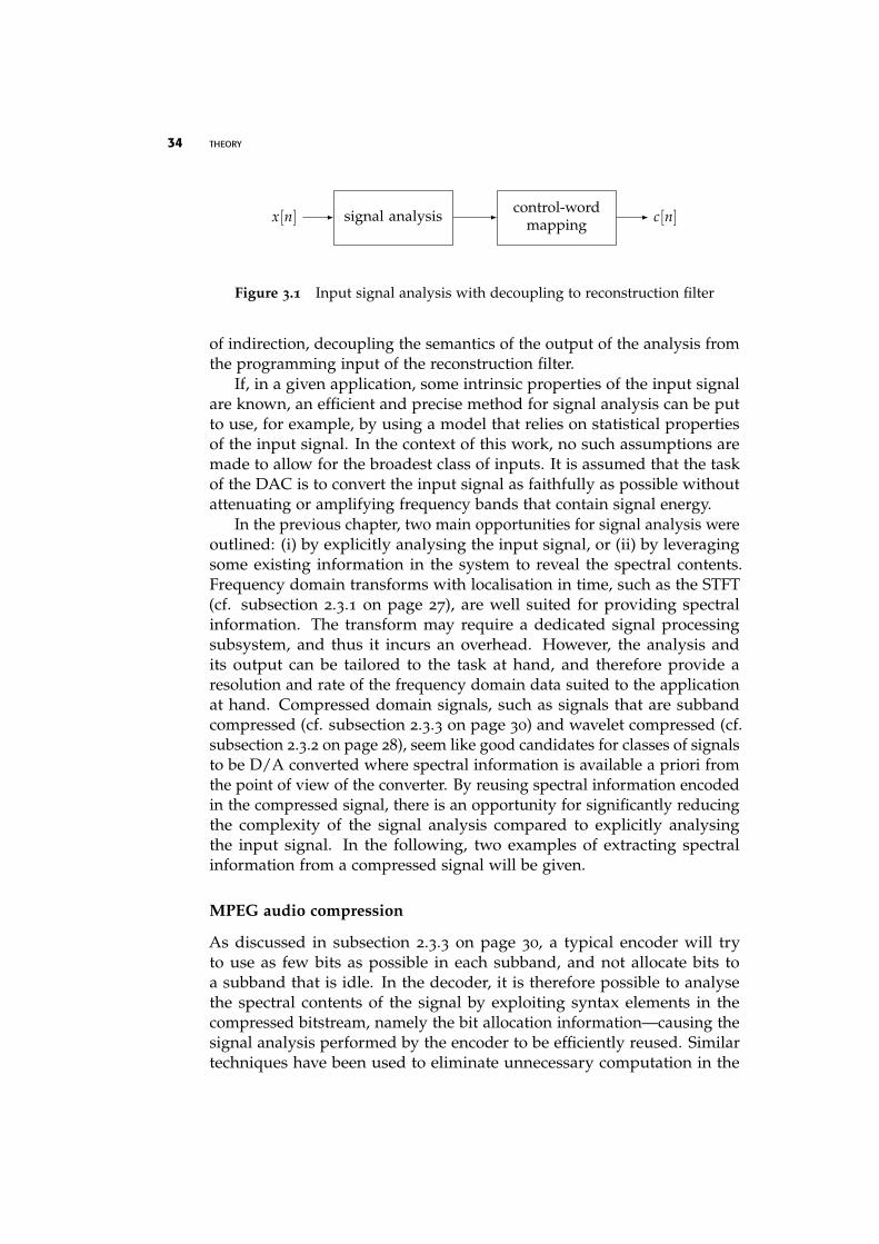
34 THEORY

x[n] signal analysis control-wordmapping c[n]

Figure 3.1 Input signal analysis with decoupling to reconstruction filter

of indirection, decoupling the semantics of the output of the analysis fromthe programming input of the reconstruction filter.

If, in a given application, some intrinsic properties of the input signalare known, an efficient and precise method for signal analysis can be putto use, for example, by using a model that relies on statistical propertiesof the input signal. In the context of this work, no such assumptions aremade to allow for the broadest class of inputs. It is assumed that the taskof the DAC is to convert the input signal as faithfully as possible withoutattenuating or amplifying frequency bands that contain signal energy.

In the previous chapter, two main opportunities for signal analysis wereoutlined: (i) by explicitly analysing the input signal, or (ii) by leveragingsome existing information in the system to reveal the spectral contents.Frequency domain transforms with localisation in time, such as the STFT(cf. subsection 2.3.1 on page 27), are well suited for providing spectralinformation. The transform may require a dedicated signal processingsubsystem, and thus it incurs an overhead. However, the analysis andits output can be tailored to the task at hand, and therefore provide aresolution and rate of the frequency domain data suited to the applicationat hand. Compressed domain signals, such as signals that are subbandcompressed (cf. subsection 2.3.3 on page 30) and wavelet compressed (cf.subsection 2.3.2 on page 28), seem like good candidates for classes of signalsto be D/A converted where spectral information is available a priori fromthe point of view of the converter. By reusing spectral information encodedin the compressed signal, there is an opportunity for significantly reducingthe complexity of the signal analysis compared to explicitly analysingthe input signal. In the following, two examples of extracting spectralinformation from a compressed signal will be given.

MPEG audio compression

As discussed in subsection 2.3.3 on page 30, a typical encoder will tryto use as few bits as possible in each subband, and not allocate bits toa subband that is idle. In the decoder, it is therefore possible to analysethe spectral contents of the signal by exploiting syntax elements in thecompressed bitstream, namely the bit allocation information—causing thesignal analysis performed by the encoder to be efficiently reused. Similartechniques have been used to eliminate unnecessary computation in the

THEORY 35

Dig

ital

sig-

nal

sou

rce

∆Σ DAC SC filter

Clocking map

y(t)

Figure 3.2 Wrapping a static bandwidth ∆Σ DAC

decoder[45]. Other works address the problem of obtaining information,such as segmentation and classification information, directly from syntaxelements in the compressed bitstream[46, 47, 48].

ECG signal compression

A wavelet-based scheme for compressing ECG signals was discussed onpage 29 of the previous chapter. The compression achieved by this approachrelies on the wavelet transform to concentrate much of the signal energyin relatively few coefficients. It was outlined how the wavelet transformcould be implemented as a filter bank where, for each level, a QMF dividesthe spectrum into a lowpass component and a highpass component. Thus,by looking at which coefficients appear in the compressed bitstream, thespectral characteristics of the ideal synthesised signal can be inferred.

3.1.2 Tunable reconstruction filter

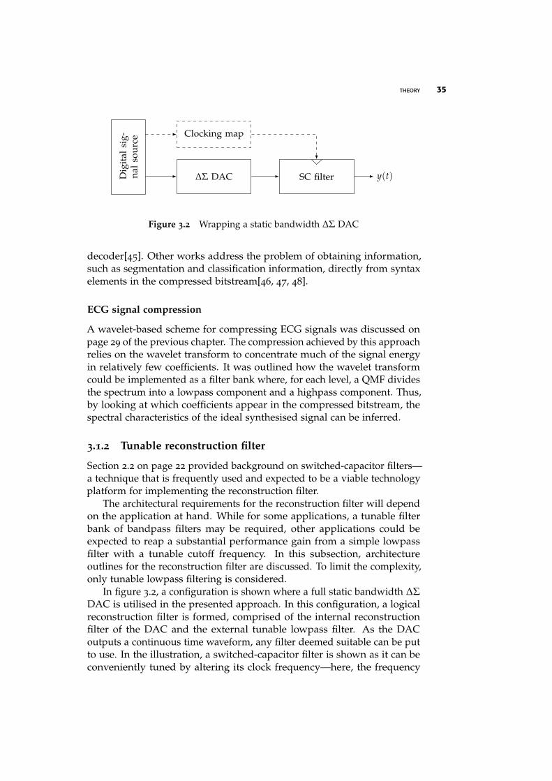
Section 2.2 on page 22 provided background on switched-capacitor filters—a technique that is frequently used and expected to be a viable technologyplatform for implementing the reconstruction filter.

The architectural requirements for the reconstruction filter will dependon the application at hand. While for some applications, a tunable filterbank of bandpass filters may be required, other applications could beexpected to reap a substantial performance gain from a simple lowpassfilter with a tunable cutoff frequency. In this subsection, architectureoutlines for the reconstruction filter are discussed. To limit the complexity,only tunable lowpass filtering is considered.

In figure 3.2, a configuration is shown where a full static bandwidth ∆ΣDAC is utilised in the presented approach. In this configuration, a logicalreconstruction filter is formed, comprised of the internal reconstructionfilter of the DAC and the external tunable lowpass filter. As the DACoutputs a continuous time waveform, any filter deemed suitable can be putto use. In the illustration, a switched-capacitor filter is shown as it can beconveniently tuned by altering its clock frequency—here, the frequency

36 THEORY

. . .

. . .

SC decimation SC filter

Clocking andtuning map

y(t)interp.filter

∆Σmod.

D/Aconv.

(a) using programmable decimation with clock tuning

. . .

. . .

SC decimation(optional) SC filter

Tuning map

y(t)interp.filter

∆Σmod.

D/Aconv.

(b) tunable filter with optional decimation

Figure 3.3 Full integration with the ∆Σ DAC

content information, provided externally, is mapped into an appropriateclock frequency for driving the switched-capacitors.

As the tunable filter is not fully integrated with the DAC, the resultingreconstruction filter is more complex than it possibly need be. Figure3.3 shows two alternative approaches. Here, the filter takes as input thesampled analogue stream from the D/A directly. As this stream is outputat a constant rate, the simple clock tuning approach presented earlieris no longer feasible. In figure 3.3a, an approach is presented wherebya programmable decimation filter adapts the sample rate to match theinput of the reconstruction filter. As the D/A converts samples at theoversampled rate, it could be convenient for some applications to decimatethe output stream before filtering[49]. However, this approach wouldrequire a programmable decimation rate, which could incur a level ofcomplexity that outweighs the potential benefit. Note that if the decimationfilter is implemented as a lowpass filter followed by a sample and holdcircuit (S/H), the bandwidth of the lowpass filter can be fixed while theS/H is used to adapt the desired output sample rate. In figure 3.3b,another potential solution is outlined whereby the D/A output is optionallydecimated at a fixed rate. Then, the result is processed by a switched-capacitor based filter with a tunable transfer function. By using a filterwith a tunable transfer function, the input rate is constant and can becustomised during design to match any desired input rate. However,circuitry for tuning the transfer function gives rise to overhead.

THEORY 37

3.1.3 Assembling the system

Two properties define the ability of the system to track spectral content inthe input signal over time: (i) The rate at which the signal analyser makesfrequency content information available, and at what rate the reconstructionfilter can be tuned. (ii) The resolution of the spectral information providedby the signal analyser, and the tuning capability of the reconstruction filter.

Some input signals may require using a programmable bandpass filterto effectively suppress quantisation noise when reconstructing the analogueoutput signal. For many applications however, a lowpass filter with atunable cutoff frequency is more realistic in terms of complexity, while stillmaking possible a substantial performance increase. Again, using MPEGaudio as an example, it can be inferred from the bit allocation tables in thestandard document[41] that the expected input signal will have most of itsenergy concentrated in the lower portion of the frequency spectrum.

Referring to figure 3.1 on page 34, the control word mapping is re-sponsible for coordinating the signal analysis effort with tuning of thereconstruction filter. To avoid unnecessary computations and complexity, itis important that the capabilities of the reconstruction filter and the signalanalysis are matched. The reconstruction filter does not need to allow forfiner grained tuning than the signal analysis is able to provide. Similarly,if the analysis rate is greater than the programming rate capability of thefilter, some of the information that has been obtained cannot be put to use.There obviously needs to be temporal correlation between the time-windowin which the signal is analysed, and when the filter is programmed. It isto be expected that a substantial SNR penalty is incurred if spectral bandsthat contain signal energy are attenuated. Thus, the filter will have to beallowed a sufficient amount of time to settle on the programmed transferfunction.

3.2 Performance gain

The basic premise underlying the presented approach is a promise ofperformance increase. In this section, the magnitude of the performancegain will be investigated by using the theoretical relations developed insubsection 2.1.5 on page 19. While it is possible that a similar approachcould be put to use to enhance other aspects of performance, such aspower consumption, only performance in terms of SNR is considered inthis report.

By referring to equations 2.13 and 2.14, it is apparent that SNR canbe improved by increasing the OSR—namely, the SNR will increase by9 dB if the OSR is doubled, in the case of a first-order noise shapingloop. The OSR was defined in equation 2.13 to be proportional to the ratio

38 THEORY

fb (kHz)

SNR (dB)

−40

−30

−20

−10

0

32

3 6 12 24

Figure 3.4 Relative SNR improvement as a function of bandwidth, fs = 384kHz

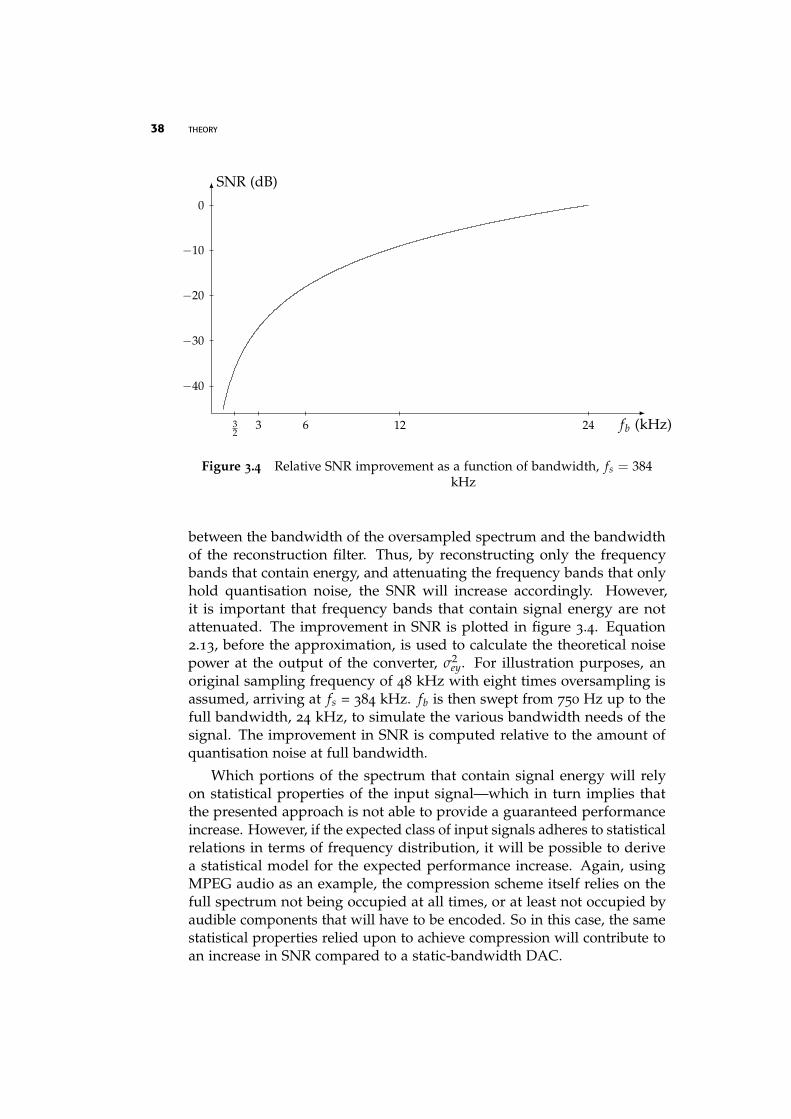
between the bandwidth of the oversampled spectrum and the bandwidthof the reconstruction filter. Thus, by reconstructing only the frequencybands that contain energy, and attenuating the frequency bands that onlyhold quantisation noise, the SNR will increase accordingly. However,it is important that frequency bands that contain signal energy are notattenuated. The improvement in SNR is plotted in figure 3.4. Equation2.13, before the approximation, is used to calculate the theoretical noisepower at the output of the converter, σ2

ey. For illustration purposes, anoriginal sampling frequency of 48 kHz with eight times oversampling isassumed, arriving at fs = 384 kHz. fb is then swept from 750 Hz up to thefull bandwidth, 24 kHz, to simulate the various bandwidth needs of thesignal. The improvement in SNR is computed relative to the amount ofquantisation noise at full bandwidth.

Which portions of the spectrum that contain signal energy will relyon statistical properties of the input signal—which in turn implies thatthe presented approach is not able to provide a guaranteed performanceincrease. However, if the expected class of input signals adheres to statisticalrelations in terms of frequency distribution, it will be possible to derivea statistical model for the expected performance increase. Again, usingMPEG audio as an example, the compression scheme itself relies on thefull spectrum not being occupied at all times, or at least not occupied byaudible components that will have to be encoded. So in this case, the samestatistical properties relied upon to achieve compression will contribute toan increase in SNR compared to a static-bandwidth DAC.

THEORY 39

By making the assumption that idle tones are equally likely to appearanywhere in the output spectrum, the dynamic adjustment of the recon-structed bandwidth will also to some extent contribute to reducing tonalityin the output noise.

This page is intentionally left blank

simulation 4

In order to quantify the performance gain experimentally and togain practical insight into implementation issues, a simulation model wasdeveloped. In this chapter, an outline is given of the simulation modelwhich is subsequently used in experiments. The experimental setup isdiscussed and results are presented.

4.1 Simulation model implementation

In this section, the implementation of the simulation model is outlinedalong with design considerations and a rationale for selecting the simulationframework.

The digital components of the simulation model were implementedusing SystemC[50]. Implemented as a framework in C++, SystemC allowsfor a smooth transition from a conceptual design through to a full customimplementation. The implemented model can start off at a high levelof abstraction emphasising architectural decisions, and may be graduallyrefined as the implementation proceeds to arrive at a cycle and bit accuratemodel suitable for synthesis by automated tools. The same testbench candrive the simulation through all stages of development, using a predefinedset of stimuli and comparing the response to an accordant golden reference.Thus, avoiding an error-prone manual translation of high-level modelsinto a register transfer level (RTL) description. An initiative is underwayto introduce analogue and mixed signal (AMS) modelling capabilities tothe SystemC framework[51]. In time, SystemC-AMS will enable seamlesssimulation of mixed signal systems. However, in its current state, SystemC-AMS is still lacking essential functionality. The work in [52] describes aseparate effort aimed at implementing an analogue modelling frameworkfor SystemC. Their implementation was however not yet publicly availablewhen the simulation model was implemented.

The simulation model developed for use in this work was implementedat the behavioural level[53], where the hardware is described algorithmi-

42 SIMULATION

cally. The model simulates an MPEG audio decoder, whose output isinterpolated and then ∆Σ modulated. The ∆Σ bitstream is subsequently fil-tered to obtain a sampled analogue output waveform∗. I.e. an MPEG audiobitstream is D/A converted by a ∆Σ DAC. A decoder capable of decodinga subset of MPEG Audio Layer II bitstreams was implemented—frameswith a monaural signal at 48 kHz sampling rate without CRC codes aresupported. The decoder was instrumented with the proposed method forobtaining spectral information. Optimisations described in [54] and [55]were applied to the subband filtering component. A multistage polyphaselowpass FIR filter was implemented to apply eight times interpolationto the output of the MPEG decoder (cf. subsection 2.1.1 on page 14). Afirst-order ∆Σ modulator was implemented to quantise and noise shapethe interpolated signal (cf. subsection 2.1.2). An output buffer was imple-mented to ensure a smooth play-out of the single bit signal from the ∆Σmodulator. These modules form the digital components of the ∆Σ DAC.Due to concerns outlined above, an ad-hoc approach was implored forsimulating the sampled data analogue reconstruction filter. The work in[1] was selected as a platform for the tunable filter due to its convenientprogrammability (cf. subsection 2.2.3). As the output rate from the D/A inthis case is 384 kHz, the charge programming circuitry needs to be clockedat close to 10 MHz. As the output rate from the D/A and the clockingfrequency for the charge programming circuit is relatively low, a decimationfilter was not deemed necessary. As close agreement between predictedand simulated performance was shown in [1], a straightforward z-domainsimulation of the lowpass IIR filter was deemed to be sufficient. As in [1],the filter has eight zeros and two poles and the coefficients were obtainedusing the approach described in [56], using software kindly provided byits author. The reconstruction filter has selectable cutoff at 750 Hz, 1500 Hz,3000 Hz, 6000 Hz, 12000 Hz, and 20250 Hz. These cutoff frequencies corre-spond to subband indices 0, 1, 3, 7, 15, and 26 in the MPEG audio bitstream.The frequency response of two of the filters is plotted in figure A.2.4 onpage 72 of the appendix. All transfer functions were designed to have apassband ripple of 1 dB and a stopband attenuation of 50 dB. Selectedsource code files are printed in section A.2 on page 57. Full simulationmodel source code is available†.

4.2 Experimental Setup

Two experiments were designed in order to indagate the performancegain experimentally by means of simulation. The first experiment uses a

∗A continuous time post filter is not part of the simulation model†http://heim.ifi.uio.no/∼jorgenam/hovedfag/model/

SIMULATION 43

synthetic input signal, and real audio data is used in the last experiment.The TwoLAME encoder∗ was used to encode the input vectors as compliantMPEG Audio Layer II bitstreams. A low bitrate was used to deliberatelystarve the encoder. If the encoder is allowed a too generous bit budget,dummy data will be encoded in order to fill the target bitrate. Thus, thebit allocation information will not convey accurate spectral information.Additionally, in a realistic audio compression scenario, the bitrate wouldbe set as low as possible. The default psychoacoustic model in TwoLAME,which is based on Psychoacoustic Model I described in Annex D of [41],was used.

For each experiment, the output of the interpolation filter and the outputof the ∆Σ modulator was stored and used as reference for the reconstructedsignal. Two reconstructed outputs were stored for comparison; one outputwhere the cutoff of the reconstruction filter was adjusted dynamicallyaccording to the proposed approach, and another output reconstructedby a filter with a fixed cutoff frequency. In addition to the output signals,the programming input of the reconstruction filter and the frequencydomain information obtained from the MPEG decoder was stored to aid insubsequent interpretation of the results. Four separate runs of the simulatorwere needed in each experiment to obtain all signals. This is not a problemas the simulation model is deterministic. After running the simulation,results from both experiments were analysed offline using a STFT, and theresulting data set was visualised as a spectrogram. As discussed in 2.3.1 onpage 27, time is on the x-axis, frequency is on the y-axis, and on the z-axis,the colour intensity represents the signal power in dB. Only a fraction ofthe oversampled spectrum is shown to emphasise the interesting details.

All simulator output data from both experiments are available†.

4.3 Results obtained from a synthetic input signal

The input vector in this experiment was a synthetic signal with a durationof five seconds encoded at 32 kbit/s. The signal contains a single tonealternating between 1 kHz and 2 kHz in one-second intervals. To avoidan overload situation in the decoder, which would result in clipping anddistortion, the synthetic signal has a time domain amplitude of 0.8. Whereasthe average power of a full scale sine wave is -3 dB, the average power ofthis signal is -4.95 dB, or -1.95 dB relative to full scale (FS)‡.

The decoded and interpolated signal is visualised as a spectrogram infigure 4.4. In this figure, the magenta-coloured line depicts the spectralinformation obtained from the decoder. Figure 4.5 depicts the output from

∗http://www.twolame.org/†http://heim.ifi.uio.no/∼jorgenam/hovedfag/results/‡−3.01 + 20 log10 0.8 = −4.95 dB

44 SIMULATION

InputOutput

t (sec)

y(t)

0.300 0.301

0.8

−0.8

(a) static (cutoff at 20250 Hz)

Input

Output

t (sec)

y(t)

0.300 0.301

0.8

−0.8

(b) dynamic (cutoff at 1500 Hz)

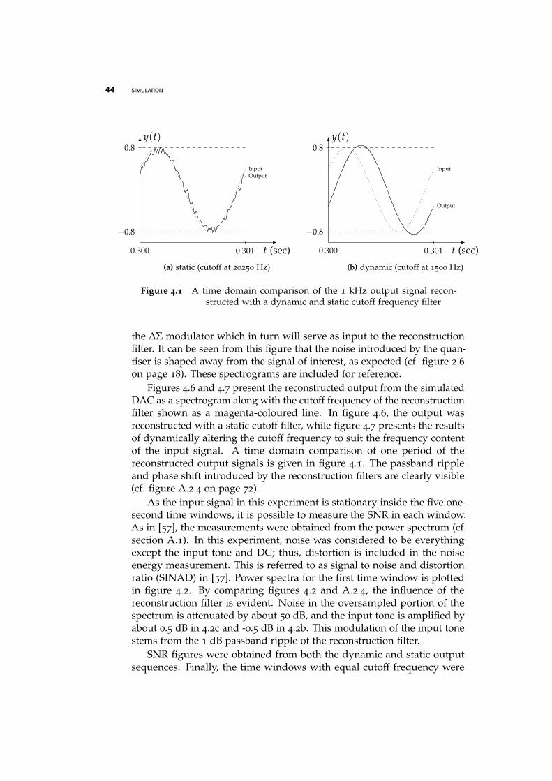
Figure 4.1 A time domain comparison of the 1 kHz output signal recon-structed with a dynamic and static cutoff frequency filter

the ∆Σ modulator which in turn will serve as input to the reconstructionfilter. It can be seen from this figure that the noise introduced by the quan-tiser is shaped away from the signal of interest, as expected (cf. figure 2.6on page 18). These spectrograms are included for reference.

Figures 4.6 and 4.7 present the reconstructed output from the simulatedDAC as a spectrogram along with the cutoff frequency of the reconstructionfilter shown as a magenta-coloured line. In figure 4.6, the output wasreconstructed with a static cutoff filter, while figure 4.7 presents the resultsof dynamically altering the cutoff frequency to suit the frequency contentof the input signal. A time domain comparison of one period of thereconstructed output signals is given in figure 4.1. The passband rippleand phase shift introduced by the reconstruction filters are clearly visible(cf. figure A.2.4 on page 72).

As the input signal in this experiment is stationary inside the five one-second time windows, it is possible to measure the SNR in each window.As in [57], the measurements were obtained from the power spectrum (cf.section A.1). In this experiment, noise was considered to be everythingexcept the input tone and DC; thus, distortion is included in the noiseenergy measurement. This is referred to as signal to noise and distortionratio (SINAD) in [57]. Power spectra for the first time window is plottedin figure 4.2. By comparing figures 4.2 and A.2.4, the influence of thereconstruction filter is evident. Noise in the oversampled portion of thespectrum is attenuated by about 50 dB, and the input tone is amplified byabout 0.5 dB in 4.2c and -0.5 dB in 4.2b. This modulation of the input tonestems from the 1 dB passband ripple of the reconstruction filter.

SNR figures were obtained from both the dynamic and static outputsequences. Finally, the time windows with equal cutoff frequency were

Power (dB)

Freq. (kHz)0 24 48 72 96 120 144 168

−100

−80

−60

−40

−20

−4.95 dB @ 1 kHz

(a) ∆Σ modulator output

Power (dB)

Freq. (kHz)0 24 48 72 96 120 144 168

−100

−80

−60

−40

−20

−5.44 dB @ 1 kHz

(b) output reconstructed with the static cutoff filter (20250 Hz)

Power (dB)

Freq. (kHz)0 24 48 72 96 120 144 168

−100

−80

−60

−40

−20

−4.45 dB @ 1 kHz

(c) output reconstructed with the dynamic cutoff filter (1500 Hz)

Figure 4.2 A frequency domain presentation of the first time window

46 SIMULATION

Table 4.1 Summary of measured results

SNR (dB)

Average Variance

Static 1000 Hz 21.89 1.69 · 10−5

2000 Hz 21.74 4.65 · 10−4

Dynamic 1000 Hz 47.11 5.55 · 10−8

2000 Hz 44.53 6.22 · 10−4

Improvement 1000 Hz 25.22 1.74 · 10−5

2000 Hz 22.79 2.16 · 10−3

averaged to obtain the results presented in table 4.1. Ideally, all SNRmeasurements in similar time windows would be equal. This is not to beexpected from practical measurements, but the underlying assumption isconfirmed by the low variance, σ2.

In the following, the measured SNR improvement is compared to theSNR improvement predicted from theory. We cannot expect the inputvector in this experiment to produce a white quantisation noise sequence,as it contains only a single tone of relatively low frequency[19]. Thus,equation 2.9 on page 20 cannot be used to obtain an accurate estimate ofthe quantisation noise power. However, equation 2.14 is still useful forpredicting the relative performance increase, since quantisation noise poweris a common factor that cancels out.

SNRdiff = SNRdynamic − SNRstatic = 10 · log10

σ2ey:static

σ2ey:dynamic

= 10 · log10fs sin(2π fb:static f−1

s )− 2π fb:static

fs sin(2π fb:dynamic f−1s )− 2π fb:dynamic

≈ 30 · log10fb:static

fb:dynamic

(4.1)

The above equation predicts a performance increase of 33.9 dB for timewindows where a cutoff frequency of 1500 Hz was selected, and 24.9 dBfor time windows reconstructed with a 3000 Hz cutoff filter. Although themeasured performance increase is lower than expected from theoreticalestimates, there is still a worthwhile performance improvement. The lowerperformance increase stems from violations of ideal theoretical assumptions;the assumption of a white quantisation noise sequence and a brick wall

SIMULATION 47

t (sec)

y(t)

0.300 0.301 0.302 0.303

0.2

−0.2

(a) static (cutoff at 20250 Hz)

t (sec)

y(t)

0.300 0.301 0.302 0.303

0.2

−0.2

(b) dynamic (cutoff at 6000 Hz)

Figure 4.3 A time domain comparison of the 2 kHz output signal recon-structed with a dynamic and static cutoff frequency filter

reconstruction filter.

4.4 Results obtained from audio data input

In this experiment, an input vector with five seconds of audio data encodedat 48 kbit/s was used. As in the previous experiment, the spectrogramsdepicting the interpolated output from the decoder and the ∆Σ modulatedbitstream are provided for reference, and plotted in figures 4.8 and 4.9.

In order to accommodate the desired bitrate, the audio encoder hasbandlimited the signal to 6 kHz, as evident by the magenta-coloured line infigure 4.8 depicting the frequency domain information obtained from thedecoder. Thus, the reconstruction filter is given an opportunity to suppressa substantial amount of quantisation noise that would otherwise have beenpresent in the output signal. As evident by comparing figures 4.10 and 4.11,there is a significant suppression of quantisation noise in the output signalreconstructed with the dynamically adapted reconstruction filter. Figure 4.4

48 SIMULATION

shows a time domain comparison of a portion of the reconstructed signal.In both plots, the dotted line represents the input to the ∆Σ modulator, andis provided for reference. The noise suppression is clearly visible in thetime domain as well.

In this experiment, the SNR improvement was not easily quantifiabledue to the non-stationary nature of the input signal.

4.5 Summary of measured results

In the preceding sections, two experiments were presented to experimen-tally verify and substantiate the promised performance increase. In the firstexperiment, the synthetic input signal was designed to be stationary insideone-second time windows. SNR figures were obtained, which demon-strated a performance increase as expected. The measured SNR figureswere also compared to theoretical estimates. In the second experiment, aperformance increase was demonstrated with real audio data, but in thiscase no SNR figures were obtained. However, a substantial suppression ofquantisation noise is evident from the visualised results.

1 2 3 4time (s)

1

5

10

20

40

1

freq

uenc

y(k

Hz)

−100

−90

−80

−70

−30

−20

−10

−0

pow

er(d

B)

Figure 4.4 Interpolated output from the MPEG audio decoder

1 2 3 4time (s)

1

5

10

20

40

1

freq

uenc

y(k

Hz)

−100

−90

−80

−70

−30

−20

−10

−0

pow

er(d

B)

Figure 4.5 Unfiltered output from the ∆Σ modulator

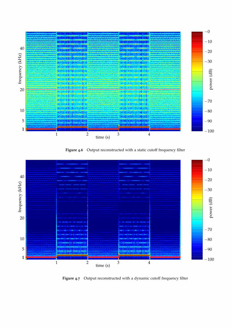
1 2 3 4time (s)

1

5

10

20

40

1

freq

uenc

y(k

Hz)

−100

−90

−80

−70

−30

−20

−10

−0

pow

er(d

B)

Figure 4.6 Output reconstructed with a static cutoff frequency filter

1 2 3 4time (s)

1

5

10

20

40

1

freq

uenc

y(k

Hz)

−100

−90

−80

−70

−30

−20

−10

−0

pow

er(d

B)

Figure 4.7 Output reconstructed with a dynamic cutoff frequency filter

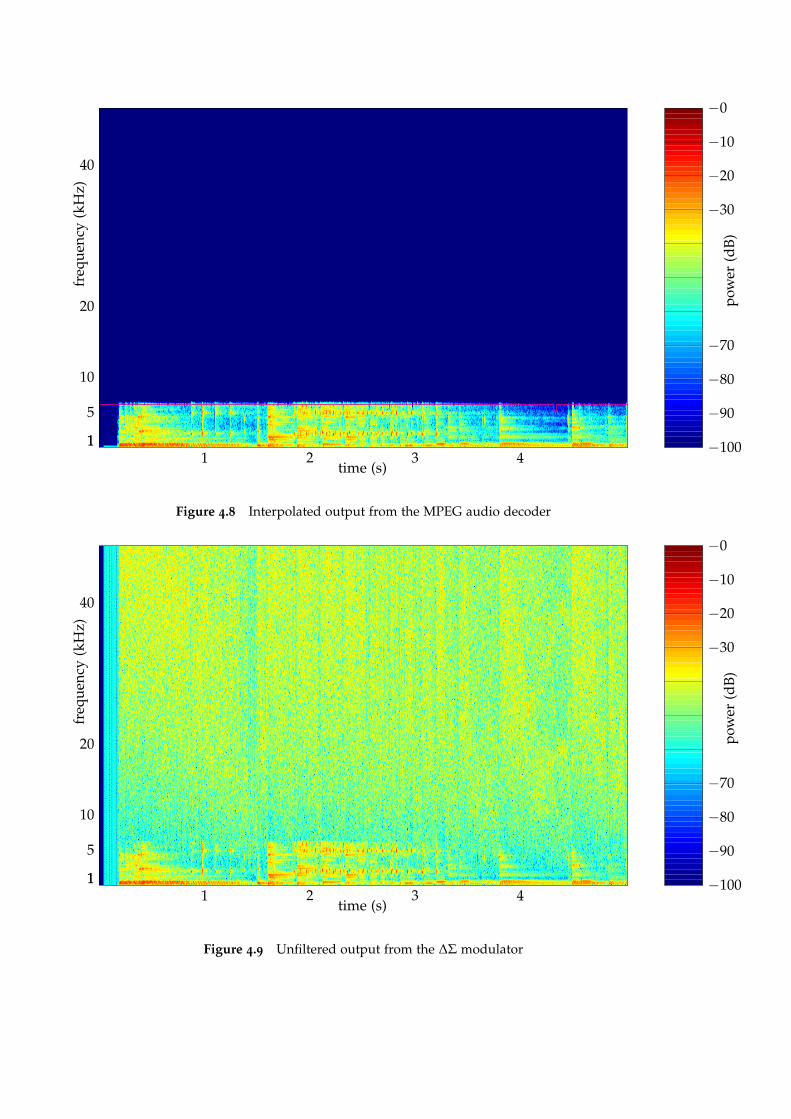
1 2 3 4time (s)

1

5

10

20

40

1

freq

uenc

y(k

Hz)

−100

−90

−80

−70

−30

−20

−10

−0

pow

er(d

B)

Figure 4.8 Interpolated output from the MPEG audio decoder

1 2 3 4time (s)

1

5

10

20

40

1

freq

uenc

y(k

Hz)

−100

−90

−80

−70

−30

−20

−10

−0

pow

er(d

B)

Figure 4.9 Unfiltered output from the ∆Σ modulator

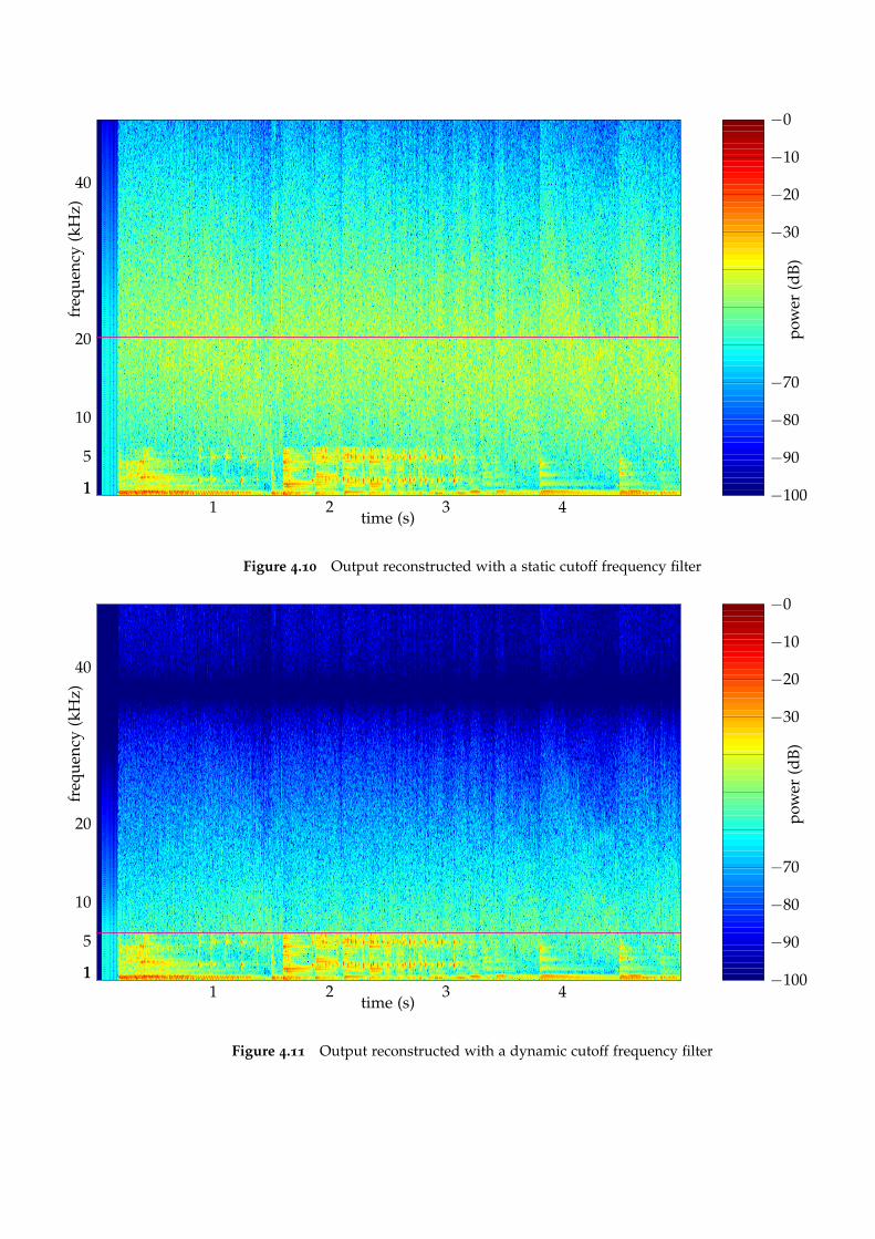
1 2 3 4time (s)

1

5

10

20

40

1

freq

uenc

y(k

Hz)

−100

−90

−80

−70

−30

−20

−10

−0

pow

er(d

B)

Figure 4.10 Output reconstructed with a static cutoff frequency filter

1 2 3 4time (s)

1

5

10

20

40

1

freq

uenc

y(k

Hz)

−100

−90

−80

−70

−30

−20

−10

−0

pow

er(d

B)

Figure 4.11 Output reconstructed with a dynamic cutoff frequency filter

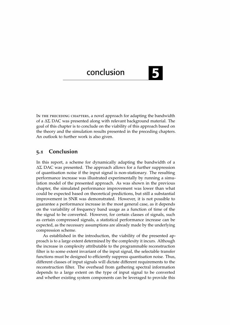
conclusion 5

In the preceding chapters, a novel approach for adapting the bandwidthof a ∆Σ DAC was presented along with relevant background material. Thegoal of this chapter is to conclude on the viability of this approach based onthe theory and the simulation results presented in the preceding chapters.An outlook to further work is also given.

5.1 Conclusion

In this report, a scheme for dynamically adapting the bandwidth of a∆Σ DAC was presented. The approach allows for a further suppressionof quantisation noise if the input signal is non-stationary. The resultingperformance increase was illustrated experimentally by running a simu-lation model of the presented approach. As was shown in the previouschapter, the simulated performance improvement was lower than whatcould be expected based on theoretical predictions, but still a substantialimprovement in SNR was demonstrated. However, it is not possible toguarantee a performance increase in the most general case, as it dependson the variability of frequency band usage as a function of time of thethe signal to be converted. However, for certain classes of signals, suchas certain compressed signals, a statistical performance increase can beexpected, as the necessary assumptions are already made by the underlyingcompression scheme.

As established in the introduction, the viability of the presented ap-proach is to a large extent determined by the complexity it incurs. Althoughthe increase in complexity attributable to the programmable reconstructionfilter is to some extent invariant of the input signal, the selectable transferfunctions must be designed to efficiently suppress quantisation noise. Thus,different classes of input signals will dictate different requirements to thereconstruction filter. The overhead from gathering spectral informationdepends to a large extent on the type of input signal to be convertedand whether existing system components can be leveraged to provide this

54 CONCLUSION

information.In summary, the presented approach can be expected to be viable if the

frequency band utilisation of the input signal is varying as a function oftime to an extent where it is not economical in some sense to allow the ∆ΣDAC to unconditionally operate at its full bandwidth, and it is convenientto obtain frequency domain information, for example by integrating theconverter with a decoder where frequency domain information is availablea priori to the system.

5.2 Future work

It is imperative to determine to what extent the adaptation introducesdistortion when the coefficients in the reconstruction filter change, and toinvestigate possible countermeasures.

A full custom prototype implementation would be interesting. Eventhough the implementation itself is a practical task without much scientificmerit, it would allow for more realistic measurements to be made. Itwould open up for a more accurate assessment of the approach, becausepower consumption can be measured and the actual increase in complexitycan be quantified. It is believed that the digital simulation modules aresynthesisable with only minor adjustments. However, some mixed signaldesign remains to be done.

In order to broaden the applicability of the approach, it is of interest toidentify other classes of input signals and compression schemes that lendsitself well to the extraction of frequency domain data.

Investigating whether it is practical to adaptively alter the noise shapingloop, H(z), is an interesting topic. If H(z) is dynamically altered to matchthe reconstruction filter by shaping the noise to bands that are attenuated,there is an opportunity for further performance increase. It is also worthinvestigating to what extent it is possible to leverage the added infrastruc-ture to accommodate the adaptive pre-amplification scheme discussed insection 1.1 on page 10, to increase the performance further without addingsignificant complexity.

Identifying to what extent there are possibilities for run-time adapta-tion of other dimensions, for example to yield an improvement in powerconsumption, is another possible future direction.

Whether the presented approach can be gainfully applied to analogueto digital converters (ADCs) is another aspect of the presented approachthat needs further investigation. The spectral information would have to beobtained from the analogue domain with low overhead. To what extent itis feasible to estimate the frequency content in the analogue input signalfrom the digital output of the ∆Σ modulator should also be looked into, asthis would reduce the complexity in the analogue domain.

source code A

A.1 Octave scripts

1 function [f,X] = fftpowerspec( x, fs, N, win )

% [f,X] = fftpowerspec -- Returns a single sided power spectrum

% representation of the time sequence x, with sampling frequency fs, using

% an N length discrete Fourier transform.

6 %

% To plot result (in dB, clipped to -120 dB):

% X_dB = max( 10 * log10(X), -120 );

% plot( f, X_dB );

%

11 % Author: Jorgen Andreas Michaelsen <jorgenam@ifi.uio.no>

% Based on: http://www.mathworks.com/support/tech-notes/1700/1702.html

if nargin < 3

16 N = length( x );

end

if nargin < 4

win = blackmanharris( length(x) );

21 end

if rem(N,2) == 1

error( ’x length must be even’ )

return;26 end

Nhalf = (N+1) / 2;

% window the signal to introduce artificial periodicity

31 x = x .* win’;

% do the actual Fourier transform using the efficient fft

X = fft( x, N );

36 % signal is real so only first part is interesting , i.e. unique

56 SOURCE CODE

X = X(1:Nhalf);

% make magnitude spectrum

X = abs( X );

41

% fft algorithm omits compensating for number of samples

X = X / length(x);

% window will introduce some loss, typically a few dB

46 X = X / mean(win);

% make the power spectrum

X = X .ˆ 2;

51 % scale since we only use one side of the spectrum,

% everything except dc and nyquist needs doubling

X(2:end-1) = X(2:end-1) * 2;

% make index to frequency map

56 f = (0:Nhalf -1) * fs / N;

function [A,pp,pf] = outputspectrogram( aufile, imgfile )

% outputspectrogram -- Make spectrogram of simulation result

4 %

% Author: Jorgen Andreas Michaelsen <jorgenam@ifi.uio.no>

[x,fs] = auload( aufile );

9 N = fs / 100; % make input tones fall dead center in a fft bin

% slice up signal in time domain and analyse each slice

% in the frequency domain

14

A = []; % the spectrogram picture

pp = []; % peak power in each slice

pf = []; % frequency of peak

19 for pos = 1:(N*0.25):(length(x)-N+1)

slice = x(pos:pos+N-1)’;

[f,X] = fftpowerspec( slice, fs, N ); % convert to power spectrum

24 % funny and useful information

[peak,pos] = max( X );

pp = [pp peak];

pf = [pf f(pos)];

29 % append this slice to the spectrogram

A = [A X’];

end

SOURCE CODE 57

34 if( nargin == 2 )

A = A(1:(N/8),:); % only a fraction of spectrum

A = max( -100, 10*log10(A) ); % make dB (clipped)

A = flipud( 64 - fix( A * 63 / (-100) ) ); % flip freqency scale

imwrite( imgfile, A, jet ); % write to image file

39 end

function fftpowerspecanalyse( f, X )

3 % fftpowerspecanalyse -- Analyse the power spectrum to obtain performance

% metrics. X is the spectral power as a function of fft bin index, and f

% is a mapping between fft bin index and frequency (in Hz).

%

% Author: Jorgen Andreas Michaelsen <jorgenam@ifi.uio.no>

8 % Based on: http://www.maxim-ic.com/appnotes.cfm/appnote_number/729

% http://www.maxim-ic.com/appnotes.cfm/appnote_number/728

span = 20; % to make a vicinity of input tone, and dc

13

% find input tone (ignoring DC)

[peakval,peakpos] = max( X(span:end) );

peakpos = peakpos + span - 1;

f_in = f(peakpos)

18 P_in = peakval

% find noise (everything else, since we count distortion as noise)

P_noi = sum( X(span:peakpos-span) );

P_noi = sum( X(peakpos+span:end) ) + P_noi

23

% performance metric

disp( ’signal to noise and distortion ratio:’ );

10 * log10( P_in / P_noi )

A.2 Simulator

Not all simulator module source code files are printed in this sectiondue to space constraints. Source code for all modules are available fromhttp://heim.ifi.uio.no/∼jorgenam/hovedfag/model/

A.2.1 Top-level

simulator.cpp

1 #include <stdio.h>

#include <string.h>

#include <signal.h>

#include <systemc.h>

6 #include "modules/leds/leds.h"

#include "modules/testbench/input.h"

#include "modules/testbench/output.h"

#include "modules/testbench/mpgout.h"

58 SOURCE CODE

#include "modules/testbench/dsmout.h"

11 #include "modules/mpeg/mpgaudparse.h"

#include "modules/mpeg/mpgaudfilter.h"

#include "modules/interp/interp.h"

#include "modules/dsmod/dsmod.h"

#include "modules/fifo/fifo.h"

16 #include "modules/recon/recon.h"

void sighandler( int signal )

{

21 sc_stop();

}

int sc_main( int argc , char **argv )

{

26 bool mpegoutput = false;bool dsmodoutput = false;bool dynamic = true;char *input_file = NULL;

char *output_file = NULL;

31 char *trace_file = NULL;

char *freq_log_file = NULL;

sc_trace_file *tf = NULL;

36 signal( SIGINT, sighandler );

signal( SIGPIPE, sighandler );

cerr << endl;

for( int i = 1; i < argc; i++ )

41 if( !strncmp("--trace=",argv[i],8) )

trace_file = argv[i] + 8;

else if( !strncmp("--input=",argv[i],8) )

input_file = argv[i] + 8;

else if( !strncmp("--output=",argv[i],9) )

46 output_file = argv[i] + 9;

else if( !strncmp("--freq-log=",argv[i],11) )

freq_log_file = argv[i] + 11;

else if( !strcmp("--mpeg-output",argv[i]) )

mpegoutput = true;51 else if( !strcmp("--dsmod-output",argv[i]) )

dsmodoutput = true;else if( !strcmp("--static",argv[i]) )

dynamic = false;else

56 cerr << "simulator: " << argv[i] << " not understood" << endl;

if( input_file != NULL )

cerr << "simulator: input " << input_file << endl;

if( output_file != NULL )

61 cerr << "simulator: output " << output_file << endl;

if( freq_log_file != NULL )

cerr << "simulator: freq log " << freq_log_file << endl;

if( trace_file != NULL )

cerr << "simulator: trace " << trace_file << endl;

66 if( mpegoutput )

cerr << "simulator: mpeg output only" << endl;

if( dsmodoutput )

cerr << "simulator: dsmod output only" << endl;

cerr << endl;

71

sc_set_default_time_unit( 1, SC_PS );

if( trace_file != NULL )

tf = sc_create_vcd_trace_file( trace_file );

76

sc_clock clock( "CLK", 434030, 0.5 );

sc_signal <bool> reset;

if( tf != NULL )

81 {

sc_trace( tf, clock.signal(), "clock" );

sc_trace( tf, reset, "reset" );

}

86 sc_signal <bool> mpeg_error;

sc_signal <bool> sync_error;

sc_signal <bool> fifo_error;

if( tf != NULL )

91 sc_trace( tf, mpeg_error , "mpeg_error" );

leds leds1( "leds" );

SOURCE CODE 59

leds1.CLK( clock );

leds1.RST( reset );

96 leds1.errSYNTAX( mpeg_error );

leds1.errBUFFER( fifo_error );

leds1.errSYNC( sync_error );

sc_signal <sc_uint <8> > bitstreambyte;

101 sc_signal <bool> ready_input;

sc_signal <sc_uint <8> > request_input;

if( tf != NULL )

{

106 sc_trace( tf, bitstreambyte , "bitstreambyte" );

sc_trace( tf, ready_input , "ready_input" );

sc_trace( tf, request_input , "request_input" );

}

111 input input1( "input_source" );

input1.CLK( clock );

input1.RST( reset );

input1.outREQ( request_input );

input1.outRDY( ready_input );

116 input1.out( bitstreambyte );

input1.set_file( input_file );

sc_signal <sc_int <17> > subbandsample;

sc_signal <bool> frame_request;

121 sc_signal <bool> subband_request;

sc_signal <bool> subband_ready;

sc_signal <sc_uint <2> > sampling_frequency;

sc_signal <sc_uint <5> > max_frequency;

126 if( tf != NULL )

{

sc_trace( tf, subbandsample , "subbandsample" );

sc_trace( tf, frame_request , "frame_request" );

sc_trace( tf, subband_request , "subband_request" );

131 sc_trace( tf, subband_ready , "subband_ready" );

}

mpgaudparse parser( "mpeg_parser" );

parser.CLK( clock );

136 parser.RST( reset );

parser.inRDY( ready_input );

parser.inREQ( request_input );

parser.in( bitstreambyte );

parser.outSAMPFREQ( sampling_frequency );

141 parser.outMAXFREQ( max_frequency );

parser.outFRAMEREQ( frame_request );

parser.outSBREQ( subband_request );

parser.outRDY( subband_ready );

parser.out( subbandsample );

146 parser.errSYNTAX( mpeg_error );

parser.errSYNC( sync_error );

sc_signal <sc_int <17> > audiosample;

sc_signal <bool> valid_audiosample;

151 sc_signal <bool> ack_audiosample;

mpgaudfilter subbandfilter( "mpeg_filter" );

subbandfilter.CLK( clock );

subbandfilter.RST( reset );

156 subbandfilter.inFRAMEREQ( frame_request );

subbandfilter.inSBREQ( subband_request );

subbandfilter.inRDY( subband_ready );

subbandfilter.in( subbandsample );

subbandfilter.outRDY( valid_audiosample );

161 subbandfilter.outACK( ack_audiosample );

subbandfilter.out( audiosample );

sc_signal <sc_int <17> > upsampledsample;

sc_signal <bool> valid_upsampledsample;

166 sc_signal <bool> ack_upsampledsample;

interp interp1( "interpolation" );

interp1.CLK( clock );

interp1.RST( reset );

171 interp1.in( audiosample );

interp1.inRDY( valid_audiosample );

interp1.inACK( ack_audiosample );

interp1.out( upsampledsample );

interp1.outRDY( valid_upsampledsample );

176 interp1.outACK( ack_upsampledsample );

60 SOURCE CODE

if( mpegoutput )

{

sc_signal <bool> valid_adaptersample;

181 sc_signal <float> adaptersample;

mpgout mpgout1( "mpeg_adapter" );

mpgout1.CLK( clock );

mpgout1.RST( reset );

186 mpgout1.in( upsampledsample );

mpgout1.inRDY( valid_upsampledsample );

mpgout1.inACK( ack_upsampledsample );

mpgout1.out( adaptersample );

mpgout1.outRDY( valid_adaptersample );

191

output output1( "output_sink" );

output1.inRST( reset );

output1.inRDY( valid_adaptersample );

output1.inFREQPROG( max_frequency );

196 output1.in( adaptersample );

output1.fixed_point_output();

output1.set_file( output_file );

output1.set_log_file( freq_log_file );

201 reset = 1;

sc_start( clock, 6 );

reset = 0;

sc_start( clock, -1 );

}

206 else if( dsmodoutput )

{

sc_signal <bool> dsmodsample;

sc_signal <bool> valid_dsmodsample;

sc_signal <bool> ack_dsmodsample;

211

dsmod dsmod1( "ds_modulator" );

dsmod1.CLK( clock );

dsmod1.RST( reset );

dsmod1.in( upsampledsample );

216 dsmod1.inRDY( valid_upsampledsample );

dsmod1.inACK( ack_upsampledsample );

dsmod1.out( dsmodsample );

dsmod1.outRDY( valid_dsmodsample );

dsmod1.outACK( ack_dsmodsample );

221

sc_signal <bool> valid_adaptersample;

sc_signal <float> adaptersample;

dsmout dsmout1( "dsm_adapter" );

226 dsmout1.CLK( clock );

dsmout1.RST( reset );

dsmout1.in( dsmodsample );

dsmout1.inRDY( valid_dsmodsample );

dsmout1.inACK( ack_dsmodsample );

231 dsmout1.out( adaptersample );

dsmout1.outRDY( valid_adaptersample );

output output1( "output_sink" );

output1.inRST( reset );

236 output1.inRDY( valid_adaptersample );

output1.inFREQPROG( max_frequency );

output1.in( adaptersample );

output1.fixed_point_output();

output1.set_file( output_file );

241 output1.set_log_file( freq_log_file );

reset = 1;

sc_start( clock, 6 );

reset = 0;

246 sc_start( clock, -1 );

}

else{

sc_signal <bool> dsmodsample;

251 sc_signal <bool> valid_dsmodsample;

sc_signal <bool> ack_dsmodsample;

dsmod dsmod1( "ds_modulator" );

dsmod1.CLK( clock );

256 dsmod1.RST( reset );

dsmod1.in( upsampledsample );

dsmod1.inRDY( valid_upsampledsample );

dsmod1.inACK( ack_upsampledsample );

dsmod1.out( dsmodsample );

261 dsmod1.outRDY( valid_dsmodsample );

SOURCE CODE 61

dsmod1.outACK( ack_dsmodsample );

sc_signal <bool> fifosample;

sc_signal <bool> clock_fifosample;

266 sc_signal <sc_uint <5> > prog_frequency;

fifo fifo1( "playout_fifo" );

fifo1.CLK( clock );

fifo1.RST( reset );

271 fifo1.in( dsmodsample );

fifo1.inRDY( valid_dsmodsample );

fifo1.inACK( ack_dsmodsample );

fifo1.inMAXFREQ( max_frequency );

fifo1.inSAMPFREQ( sampling_frequency );

276 fifo1.out( fifosample );

fifo1.outCLK( clock_fifosample );

fifo1.outMAXFREQ( prog_frequency );

fifo1.errBUFFER( fifo_error );

281 sc_signal <float> outsample;

recon recon1( "reconstruction" );

recon1.inRST( reset );

recon1.inCLK( clock_fifosample );

286 recon1.inFREQPROG( prog_frequency );

recon1.in( fifosample );

recon1.out( outsample );

if( dynamic )

recon1.set_dynamic();

291 elserecon1.set_static();

output output1( "output_sink" );

output1.inRST( reset );

296 output1.inRDY( clock_fifosample );

output1.inFREQPROG( prog_frequency );

output1.in( outsample );

output1.floating_point_output();

output1.set_file( output_file );

301 output1.set_log_file( freq_log_file );

reset = 1;

sc_start( clock, 6 );

reset = 0;

306 sc_start( clock, -1 );

}

cerr << "simulation ends at " << (sc_time_stamp().to_seconds()*1000);

cerr << " ms" << endl;

311

return 0;

}

A.2.2 MPEG audio parser

mpgaudparse.h

#define CACHE_SIZE 256 // words

2

SC_MODULE( mpgaudparse )

{

sc_in<bool> RST;

7

sc_out<sc_uint <8> > inREQ;

sc_in<bool> inRDY;

sc_in<sc_uint <8> > in;

12 sc_out<sc_uint <5> > outMAXFREQ;

sc_out<sc_uint <2> > outSAMPFREQ;

sc_in<bool> outFRAMEREQ;

sc_in<bool> outSBREQ;

sc_out<bool> outRDY;

17 sc_out<sc_int <17> > out;

sc_out<bool> errSYNTAX;

sc_out<bool> errSYNC;

22 sc_in_clk CLK;

sc_uint <32> cache[CACHE_SIZE];

62 SOURCE CODE

sc_uint <8> cache_rd_pos;

sc_uint <8> cache_wr_pos;

27 sc_uint <32> cache_word;

sc_uint <6> cache_wordpos;

SC_CTOR( mpgaudparse )

32 {

SC_CTHREAD( run, CLK.pos() );

watching( RST.delayed() == true );

}

37 void run( void );

void write_sample( sc_int <17> );

sc_uint <16> read_sample_code( sc_uint <5> );

sc_uint <16> get_next_word( sc_uint <5> );

bool get_next_bit( void );

42 void refresh_cache( void );

void mpgaudparse::fill_cache( void );

sc_int <17> invq( sc_uint <16>, sc_uint <4>, sc_uint <5> );

};

mpgaudparse.cpp

#include <stdio.h>

#include <systemc.h>

#include "mpgaudparse.h"

5 #include "mpgscale.h"

#include "mpginvq.h"

#include "mpgalloc.h"

#include "mpggrouped.h"

10 #define MPEG_ERROR { errSYNTAX.write( true ); wait(); continue; }

#define SYNCPATTERN 0xFFFFFF

#define SBLIMIT 32

15

bool mpgaudparse::get_next_bit( void )

{

if( cache_wordpos == 0 )

refresh_cache();

20

cache_wordpos --;

return cache_word & (1<<cache_wordpos) ? 1 : 0;

}

25

sc_uint <16> mpgaudparse::read_sample_code( sc_uint <5> num_bits )

{

sc_uint <16> sample_code = 0; // 16 bit

30

if( cache_wordpos < num_bits )

{

num_bits -= cache_wordpos;

sample_code = get_next_word( cache_wordpos ) << num_bits;

35 refresh_cache();

sample_code |= get_next_word( num_bits );

}

elsesample_code = get_next_word( num_bits );

40

return sample_code;

}

45 sc_uint <16> mpgaudparse::get_next_word( sc_uint <5> num_bits )

{

sc_uint <32> mask = (1<<num_bits) - 1;

cache_wordpos -= num_bits;

50 mask <<= cache_wordpos;

mask &= cache_word;

mask >>= cache_wordpos;

mask &= 0xFFFF;

55 return mask;

}

SOURCE CODE 63

void mpgaudparse::refresh_cache( void )

60 {

cache_word = cache[cache_rd_pos];

if( cache_rd_pos == CACHE_SIZE - 1 )

cache_rd_pos = 0;

65 elsecache_rd_pos++;

cache_wordpos = 32;

}

70

void mpgaudparse::fill_cache( void )

{

unsigned char req_size = 0;

75

if( cache_rd_pos == cache_wr_pos )

// this only happens on reset

req_size = CACHE_SIZE - 1;

else if( cache_rd_pos < cache_wr_pos )

80 req_size = CACHE_SIZE - 1 - cache_wr_pos + cache_rd_pos;

else /* if( cache_rd_pos > cache_wr_pos ) */req_size = cache_rd_pos - cache_wr_pos - 1;

inREQ.write( req_size );

85 wait_until( inRDY.delayed() == true );

inREQ.write( 0 );

for( int i = 0; i <= req_size; i++ )

90 {

cache[cache_wr_pos] = 0;

cache[cache_wr_pos] |= (in.read() << 24) & 0xFF000000;

wait();

95 cache[cache_wr_pos] |= (in.read() << 16) & 0x00FF0000;

wait();

cache[cache_wr_pos] |= (in.read() << 8) & 0x0000FF00;

wait();

cache[cache_wr_pos] |= in.read() & 0x000000FF;

100 wait();

if( cache_wr_pos == CACHE_SIZE - 1 )

cache_wr_pos = 0;

else105 cache_wr_pos++;

}

wait();

}

110

sc_int <17> mpgaudparse::invq( sc_uint <16> qsample, sc_uint <4> msb,

sc_uint <5> index )

{

115 sc_int <33> value;

value = (qsample & ((1<<msb)-1)) << (16-msb);

120 if( !(qsample & (1<<msb)) )

value -= 1 << 16;

value += invq_D[index];

value *= invq_C[index];

125 value /= ((1<<16)-1);

return value;

}

130

void mpgaudparse::run( void )

{

unsigned int framecount;

unsigned int table_select = 0;

135 bool protection_bit;

sc_uint <4> bitrate;

sc_uint <5> max_frequency;

sc_uint <2> sampling_frequency;

140 sc_uint <5> allocation[SBLIMIT]; // 2..4 bits

sc_uint <6> scale_factor[SBLIMIT][3];

64 SOURCE CODE

sc_int <17> frame_sample[SBLIMIT][3];

145

framecount = 0;

cache_rd_pos = 0;

cache_wr_pos = 0;

cache_wordpos = 0;

150

out.write( 0 );

outRDY.write( false );

inREQ.write( 0 );

errSYNC.write( false );

155

wait();

// Frame loop

160

while( 1 )

{

errSYNTAX.write( false );

165 fill_cache();

// We decode MPEG-1 layer II, so start of frame contains

// 14 one-bits (sync + id + first bit of layer).

170 for( int i = 0; i < 14; i++ )

{

if( get_next_bit() == 0 )

{

errSYNC.write( true );

175 i = -1;

}

wait();

}

180

wait();

errSYNC.write( false );

185

// Expect a zero-bit next (layer II), otherwise find next frame

if( get_next_bit() != 0 )

MPEG_ERROR

190

// protection_bit

protection_bit = !get_next_bit();

195 // bitrate, we support 32 kbps up to 192 kbps

bitrate = get_next_bit() << 3;

bitrate |= get_next_bit() << 2;

bitrate |= get_next_bit() << 1;

200 bitrate |= get_next_bit();

if( bitrate == 1 || bitrate == 2 )

table_select = 1;

else if( bitrate >= 3 && bitrate <= 10 )

205 table_select = 0;

elseMPEG_ERROR

// sampling frequency , we only support 48 kHz

210

sampling_frequency = get_next_bit() << 1;

sampling_frequency |= get_next_bit();

if( sampling_frequency != 1 )

215 MPEG_ERROR

outSAMPFREQ.write( sampling_frequency );

// ignore padding and private

220

for( int i = 0; i < 2; i++ )

get_next_bit();

// mode must be mono

225

if( get_next_bit() != 1 || get_next_bit() != 1 )

SOURCE CODE 65

MPEG_ERROR

// ignore mode extension , copyright and original

230

for( int i = 0; i < 4; i++ )

get_next_bit();

// we require "no emphasis"

235

if( get_next_bit() != 0 || get_next_bit() != 0 )

MPEG_ERROR

// skip crc (if any)

240

if( protection_bit )

{

for( int i = 0; i < 16; i++ )

get_next_bit();

245

wait();

}

// we are now ready for frame data

250

// read bit allocation information

max_frequency = 0;

outMAXFREQ.write( 0 );

255 for( int sb = 0; sb < SBLIMIT; sb++ )

{

sc_uint <4> alloc = 0;

switch( quant_alloc_table[table_select][sb][0] )

{

260 case 4:

alloc |= get_next_bit() << 3;

case 3:

alloc |= get_next_bit() << 2;

case 2:

265 alloc |= get_next_bit() << 1;

alloc |= get_next_bit();

}

if( alloc == 0 )

270 allocation[sb] = 0;

else{

allocation[sb] = quant_alloc_table[table_select][sb][alloc];

max_frequency = sb;

275 outMAXFREQ.write( sb );

}

wait();

}

280

wait();

cerr << "mpgaudparse: " << outMAXFREQ.read() << endl;

285

// read scalefactor grouping information

for( int sb = 0; sb < SBLIMIT; sb++ )

{

290 if( allocation[sb] != 0 )

{

scale_factor[sb][2] = get_next_bit() << 1;

scale_factor[sb][2] |= get_next_bit();

}

295

wait();

}

wait();

300

// read actual scale factors

for( int sb = 0; sb < SBLIMIT; sb++ )

305 {

if( allocation[sb] != 0 )

{

scale_factor[sb][0] = read_sample_code( 6 );

310 switch( scale_factor[sb][2] )

66 SOURCE CODE

{

case 0:

// (one) (two) (three)

scale_factor[sb][1] = read_sample_code( 6 );

315 scale_factor[sb][2] = read_sample_code( 6 );

break;

case 1:

// (one two) (three)

320 scale_factor[sb][1] = scale_factor[sb][0];

scale_factor[sb][2] = read_sample_code( 6 );

break;

case 2:

325 // (one two three)

scale_factor[sb][1] = scale_factor[sb][0];

scale_factor[sb][2] = scale_factor[sb][0];

break;

330 case 3:

// (one) (two three)

scale_factor[sb][1] = read_sample_code( 6 );

scale_factor[sb][2] = scale_factor[sb][1];

break;335 }

}

wait();

}

340

wait();

// output frame sync and frequency info

345

wait_until( outFRAMEREQ.delayed() == true );

outRDY.write( true );

out.write( SYNCPATTERN );

350 wait();

outRDY.write( false );

// read quantised sample codes, dequantise and scale

355

for( int gr = 0; gr < 12; gr++ )

{

for( int sb = 0; sb < SBLIMIT; sb++ )

{

360 int alloc_index = allocation[sb];

if( alloc_index != 0 )

{

sc_uint <16> qsample;

365 if( alloc_index < 4 ) // if grouping

{

sc_uint <4> nlevels =

quant_grouped_table[alloc_index][0];

370 sc_uint <10> c =

read_sample_code( quant_grouped_table[alloc_index][1]);

for( int s = 0; s < 3; s++ ) // unroll

{ // degroup

375 qsample = c % nlevels;

c /= nlevels;

frame_sample[sb][s] =

invq( qsample, alloc_index , alloc_index - 1 );

380 }

}

else // no grouping , read three samples{

for( int s = 0; s < 3; s++ ) // unroll

385 {

qsample = read_sample_code( alloc_index - 1 );

frame_sample[sb][s] =

invq( qsample, alloc_index - 2, alloc_index - 1 );

390 }

}

// denormalise

for( int s = 0; s < 3; s++ ) // unroll

SOURCE CODE 67

395 {

sc_int <42> product;

product = frame_sample[sb][s] *

scale_factor_table[scale_factor[sb][gr>>2]];

400

product >>= 23;

// if neccessary , clip

if( product > ((1<<16)-1) )

405 product = (1<<16) - 1;

else if( product < -(1<<16) )

product = -(1<<16);

frame_sample[sb][s] = product;

410 }

}

elsefor( int s = 0; s < 3; s++ ) // unroll

frame_sample[sb][s] = 0;

415 }

// output samples (to be read by filterbank)

420 for( int s = 0; s < 3; s++ ) // unroll

{

wait_until( outSBREQ.delayed() == true );

outRDY.write( true );

425 for( int sb = 0; sb < SBLIMIT; sb++ )

{

out.write( frame_sample[sb][s] );

wait();

outRDY.write( false );

430 }

wait();

}

}

435 }

}

A.2.3 ∆Σ modulator

dsmod.h

SC_MODULE( dsmod )

{

sc_in<bool> RST;

4

sc_out<bool> inACK;

sc_in<bool> inRDY;

sc_in<sc_int <17> > in;

9 sc_in<bool> outACK;

sc_out<bool> outRDY;

sc_out<bool> out;

sc_in_clk CLK;

14

SC_CTOR( dsmod )

{

SC_CTHREAD( run, CLK.pos() );

19 watching( RST.delayed() == true );

}

void run( void );

};

dsmod.cpp

#include <systemc.h>

2 #include "dsmod.h"

void dsmod::run( void )

{

7 sc_int <32> u;

68 SOURCE CODE

sc_int <32> v;

sc_int <17> x;

bool y;

sc_uint <32> o;

12

v = 0;

y = false;

17 out.write( y );

outRDY.write( false );

inACK.write( false );

wait();

22

while( 1 )

{

// wait until interpolation filter is ready

// to burst data

27

inACK.write( true );

wait_until( inRDY.delayed() == true );

32 // read and compute

o = 0;

for( unsigned int i = 0; i < 32; i++ )

37 {

x = in.read();

if( y )

u = x - 32767;

42 elseu = x + 32768;

v = u + v;

47 y = 0;

if( v >= 0 )

{

y |= 1;

o |= 1 << i;

52 }

wait();

57 inACK.write( false );

}

// write

62

outRDY.write( true );

out.write( (o & 1) != 0 );

wait_until( outACK.delayed() == true );

outRDY.write( false );

67

for( unsigned int i = 1; i < 32; i++ )

{

out.write( (o & (1<<i)) != 0 );

wait();

72 }

}

}

A.2.4 Reconstruction filter

filterdef.h

1 // *********************************************************

//

// 750 Hz:

// [b,a] = iirremez( 8, 2, 1, 1/32/8, 0.035+1/32/8 );

// The stopband attenuation is 50.024823

6 //

// 1500 Hz:

// [b,a] = iirremez( 8, 2, 1, 2/32/8, 0.065+2/32/8 );

// The stopband attenuation is 50.495655

//

SOURCE CODE 69

11 // 3000 Hz:

// [b,a] = iirremez( 8, 2, 1, 4/32/8, 0.1+4/32/8 );

// The stopband attenuation is 50.088281

//

// 6000 Hz:

16 // [b,a] = iirremez( 8, 2, 1, 8/32/8, 0.145+8/32/8 );

// The stopband attenuation is 50.569357

//

// 12000 Hz:

// [b,a] = iirremez( 8, 2, 1, 16/32/8, 0.185+16/32/8 );

21 // The stopband attenuation is 50.706724

//

// 20250 Hz: (because sbmax is 27 for the streams we decode)

// [b,a] = iirremez( 8, 2, 1, 27/32/8, 0.2+27/32/8 );

// The stopband attenuation is 50.530362

26 //

// *********************************************************

31 const double a[6][N] =

{

{ 1.00000000000000e+00, -1.98828051035226e+00, 9.88423710082639e-01 },

{ 1.00000000000000e+00, -1.97307964507895e+00, 9.73733396241935e-01 },

{ 1.00000000000000e+00, -1.94581629875807e+00, 9.48410232837472e-01 },

36 { 1.00000000000000e+00, -1.89029384083126e+00, 9.00547778618750e-01 },

{ 1.00000000000000e+00, -1.77876514486171e+00, 8.18906519700735e-01 },

{ 1.00000000000000e+00, -1.63233798856964e+00, 7.43344054934946e-01 }

};

41

const double b[6][M] =

{

{ 1.79096577699688e-03, -3.10533649328450e-03, 1.37599093960560e-03,

4.12406373687460e-06, 3.78330794301216e-06, 3.97629867362051e-06,

46 1.37595758093198e-03, -3.10515271483066e-03, 1.79088048886445e-03 },

{ 1.92657804346049e-03, -2.82507355539670e-03, 1.15881235059790e-03,

3.21418411545018e-05, 3.22765521365358e-05, 3.21246037557058e-05,

1.15878541806046e-03, -2.82501166268633e-03, 1.92654719105031e-03 },

51

{ 2.42218838018840e-03, -2.62579609088878e-03, 1.14170817229617e-03,

1.89949528960408e-04, 1.92579998132317e-04, 1.90139029412703e-04,

1.14147563452980e-03, -2.62557242308833e-03, 2.42207165370041e-03 },

56 { 3.09437959409010e-03, -1.43369842877068e-03, 1.59416188984010e-03,

1.04649196754133e-03, 1.07770452224338e-03, 1.04659867717741e-03,

1.59393671497599e-03, -1.43348986709300e-03, 3.09426200330691e-03 },

{ 4.59313739737402e-03, 1.68310066593505e-03, 4.78048733019410e-03,

61 5.16803093221080e-03, 5.44537485246289e-03, 5.16812040045895e-03,

4.78020008924796e-03, 1.68329093110759e-03, 4.59292409775701e-03 },

{ 6.82953391841229e-03, 7.50600047854121e-03, 1.31862384813037e-02,

1.61816211866498e-02, 1.73914693545687e-02, 1.61816889084217e-02,

66 1.31855252324219e-02, 7.50611033116081e-03, 6.82896777694246e-03 }

};

recon.h

#define M 9

#define N 3

3

SC_MODULE( recon )

{

sc_in<sc_uint <5> > inFREQPROG;

sc_in<bool> inCLK;

8 sc_in<bool> inRST;

sc_in<bool> in;

sc_out<float> out;

13

unsigned int select;

unsigned int freq;

unsigned int t;

bool dynamic;

18

double x[M];

double y[N];

23 SC_CTOR( recon )

70 SOURCE CODE

{

SC_METHOD( entry );

sensitive << inCLK.pos() << inRST.pos();

}

28

void entry( void );

void set_dynamic( void );

void set_static( void );

};

recon.cpp

#include <systemc.h>

3 #include "recon.h"

#include "filterdef.h"

#define XIDX(i) ((i+t)%M)

8 #define YIDX(i) ((i+t)%N)

#define X(i) x[XIDX(i)]

#define Y(i) y[YIDX(i)]

13

void recon::set_static( void )

{

dynamic = false;}

18

void recon::set_dynamic( void )

{

dynamic = true;}

23

void recon::entry( void )

{

if( inRST.read() )

{

28 select = 5;

freq = 0;

t = 0;

for( int i = 0; i < N; i++ )

33 y[i] = 0;

for( int i = 0; i < M; i++ )

x[i] = 0;

38 return;}

// update time, then input

43

t++;

if( t == 9 )

t = 0;

48 if( in.read() )

X(0) = 1.0;

elseX(0) = -1.0;

53 if( dynamic && inFREQPROG.read() != freq )

{

freq = inFREQPROG.read();

if( freq <= 0 )

58 select = 0;

else if( freq <= 1 )

select = 1;

else if( freq <= 3 )

select = 2;

63 else if( freq <= 7 )

select = 3;

else if( freq <= 15 )

select = 4;

else68 select = 5;

}

SOURCE CODE 71

Y(0) = 0;

73

// compute new output

for( int k = 0; k < M; k++ )

Y(0) += b[select][k] * X(M-k);

78

for( int k = 1; k < N; k++ )

Y(0) -= a[select][k] * Y(N-k);

Y(0) /= a[select][0];

83

out.write( Y(0) );

}

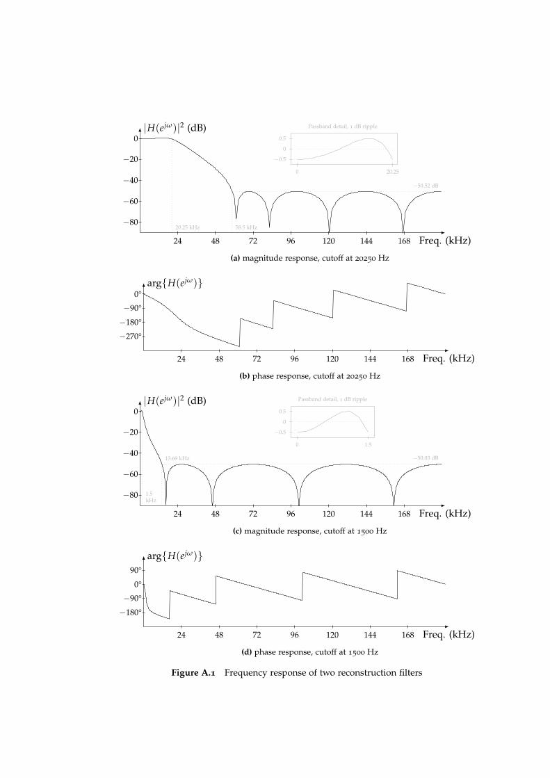
−80

−60

−40

−20

0

24 48 72 96 120 144 168

58.5 kHz

−50.52 dB

20.25 kHz

|H(ejω)|2 (dB)

Freq. (kHz)

Passband detail, 1 dB ripple

0.5

−0.5

0

0 20.25

(a) magnitude response, cutoff at 20250 Hz

Freq. (kHz)

arg{H(ejω)}

24 48 72 96 120 144 168

−270°

−180°

−90°

0°

(b) phase response, cutoff at 20250 Hz

−80

−60

−40

−20

0

24 48 72 96 120 144 168

13.69 kHz −50.03 dB

1.5kHz

|H(ejω)|2 (dB)

Freq. (kHz)

Passband detail, 1 dB ripple

0.5

−0.5

0

0 1.5

(c) magnitude response, cutoff at 1500 Hz

Freq. (kHz)

arg{H(ejω)}

24 48 72 96 120 144 168

−180°

−90°

0°

90°

(d) phase response, cutoff at 1500 Hz

Figure A.1 Frequency response of two reconstruction filters

bibliography

[1] Joarez B. Monteiro, Antonia Petaglia, and Carlos A. Leme. CapacitorCharge Control Technique Applied to Digitally Programmable IIRSwitched-Capacitor Filter. In 15th Symposium on Integrated Circuits andSystems Design, pages 68–73. IEEE Computer Society, September 2002.

[2] Chris Dunn and Mark Sandler. Adaptive sigma-delta modulation foruse in DACs. Electronics Letters, 32(10):867–868, May 1996.

[3] M. C. Ramesh and K. S. Chao. Sigma Delta Analog to Digital Con-verters with Adaptive Quantization. In Proceedings of the 40th MidwestSymposium on Circuits and Systems, 1997, volume 1, pages 22–25. IEEE,August 1997.

[4] Clemens M. Zierhofer. Adaptive Sigma-Delta Modulation With One-Bit Quantization. IEEE Transactions on Circuits and Systems—II: Analogand Digital Signal Processing, 47(5):408–415, May 2000.

[5] Mansour A. Aldajani and Ali H. Sayed. Stability and PerformanceAnalysis of an Adaptive Sigma-Delta Modulator. IEEE Transactions onCircuits and Systems—II: Analog and Digital Signal Processing, 48(3):233–243, March 2001.

[6] Steven R. Norsworthy. Quantization Errors and Dithering in ∆Σ Modu-lators. In Steven R. Norsworthy, Richard Schreier, and Gabor C. Temes,editors, Delta-Sigma Data Converters: Theory, Design, and Simulation,chapter 3, pages 75–140. IEEE Press, 1997.

[7] Jouko Vankka, Jonne Lindeberg, and Kari Halonen. A Direct DigitalSynthesizer with Tunable Delta Sigma Modulator. Analog IntegratedCircuits and Signal Processing, 38(1):7–15, January 2004.

[8] J. C. Candy. An Overview of Basic Consepts. In Steven R. Norswor-thy, Richard Schreier, and Gabor C. Temes, editors, Delta-Sigma DataConverters: Theory, Design, and Simulation, chapter 1, pages 1–43. IEEEPress, 1997.

74 BIBLIOGRAPHY

[9] Sanjit K. Mitra. Digital Signal Processing. McGraw-Hill, second edition,2001.

[10] Yrjo Neuvo, Dong Cheng-Yu, and Sanjit K. Mitra. Interpolated FiniteImpulse Response Filters. IEEE Transactions on Acoustics, Speech, andSignal Processing, 32(3):536–570, June 1984.

[11] Brian P. Brandt and Bruce A. Wooley. A Low-Power, Area-EfficientDigital Filter for Decimation and Interpolation. IEEE Journal of Solid-State Circuits, 29(6):679–687, June 1994.

[12] Eugene B. Hogenauer. An Economical Class of Digital Filters forDecimation and Interpolation. IEEE Transactions on Acoustics, Speech,and Signal Processing, 29(2):155–162, 1981.

[13] Robert W. Adams and Richard Schreier. Stability Theory for ∆Σ Modu-lators. In Steven R. Norsworthy, Richard Schreier, and Gabor C. Temes,editors, Delta-Sigma Data Converters: Theory, Design, and Simulation,chapter 4, pages 141–164. IEEE Press, 1997.

[14] Pervez M. Aziz, Henrik V. Sorensen, and Jan van der Spiegel. AnOverview of Sigma-Delta Converters. IEEE Signal Processing Magazine,13(1):61–84, January 1996.

[15] Mucahit Kozak and Izzet Kale. Oversampled Delta-Sigma Modulators.Kluwer Academic Publishers, 2003.

[16] Anekal B. Sripad and Donald L. Snyder. A Necessary and SufficientCondition for Quantization Errors to be Uniform and White. IEEETransactions on Acoustics, Speech, and Signal Processing, 25(5):442–448,October 1977.

[17] Monson H. Hayes. Statistical Digital Signal Processing and Modeling.John Wiley & Sons, Inc., 1996.

[18] Robert M. Gray. Spectral Analysis of Quantization Noise in a Single-Loop Sigma-Delta Modulator with DC Input. IEEE Transactions onCommunications, 37(6):588–599, June 1989.

[19] Robert M. Gray, Wu Chou, and Ping W. Wong. Quantization Noisein Single-Loop Sigma-Delta Modulation with Sinusoidal Inputs. IEEETransactions on Communications, 37(9):956–968, September 1989.

[20] Richard Schreier. On the Use of Chaos to Reduce Idle-Channel Tonesin Delta-Sigma Modulators. IEEE Transactions on Circuits and Systems—I: Fundamental Theory and Applications, 41(8):539–547, August 1994.

BIBLIOGRAPHY 75

[21] Chris Dunn and Mark Sandler. Linearising Sigma-Delta Modulatorsusing Dither and Chaos. In 1995 IEEE International Symposium onCircuits and Systems, volume 1, pages 625–628. IEEE, 1995.

[22] J. B. Hughes and A. Worapishet. Switched Capacitors or SwitchedCurrent—Which Will Succeed? In Chris Toumazou, George S.Moschytz, and Barrie Gilbert, editors, Trade-Offs in Analog CircuitDesign, chapter 11. Springer, first edition, October 2002.

[23] Roubik Gregorian and Gabor C. Temes. Analog MOS Integrated Circuitsfor Signal Processing. Wiley, 1986.

[24] Christian C. Enz and Gabor C. Temes. Circuit Techniques for Re-ducing the Effects of Op-Amp Imperfections. Proceedings of the IEEE,84(11):1584–1614, November 1996.

[25] Alan Hastings. The Art of Analog Layout. Prentice Hall, 2001.

[26] Paul J. Hurst and James E. C. Brown. Finite Impulse ResponseSwitched-Capacitor Decimation Filters for the DSM D/A Interface. InIEEE International Symposium on Circuits and Systems, volume 3, pages1688–1691. IEEE, May 1989.

[27] Mikael Gustavsson and Nianxiong Nick Tan. Decimating SC filterfor high speed Sigma-Delta D/A converters. In Proceedings of the2004 International Symposium on Circuits and Systems, volume 1, pages657–660. IEEE, May 2004.

[28] A. Petraglia, J.S. Pereira, and F.A.P. Baruqui. Low-sensitivity IIRswitched-capacitor decimation filters using delay lines with staggeredT/H stages. IEE Proceedings – Circuits, Devices and Systems, 153(2):193–198, April 2006.

[29] Un-Ku Moon. CMOS High-Frequency Switched-Capacitor Filters forTelecommunication Applications. IEEE Journal of Solid-State Circuits,35(2):212–220, February 2000.

[30] Franklin F. Kuo. Network Analysis and Synthesis, chapter 3. John Wiley& Sons, Inc., second edition, 1966.

[31] W. Kenneth Jenkins. Fourier Series, Fourier Transforms, and the DFT.In Wai-Kai Chen, editor, The Circuits and Filters Handbook, volume 28 ofElectrical Engineering Handbook, chapter 4. CRC Press, second edition,2003.

[32] James W. Cooley and John W. Tukey. An Algorithm for the MachineCalculation of Complex Fourier Series. Mathematics of Computation,19(90):297–301, 1965.

76 BIBLIOGRAPHY

[33] Frederic J. Harris. On the Use of Windows for Harmonic Analysis withthe Discrete Fourier Transform. Proceedings of the IEEE, 66(1):51–83,January 1978.

[34] Magdy T. Hanna. Windows with Rapidly Decaying Sidelobes andSteerable Sidelobe Dips. IEEE Transactions on Signal Processing,42(5):2037–2044, August 1994.

[35] P. P. Vaidyanathan and Igor Djokovic. Wavelet Transforms. In Wai-KaiChen, editor, The Circuits and Filters Handbook, volume 28 of ElectricalEngineering Handbook, chapter 6. CRC Press, second edition, 2003.

[36] Gilbert Strang and Truong Nguyen. Wavelets and Filter Banks. Wellesley-Cambridge Press, 1996.

[37] Paul S. Addison. Wavelet transforms and the ECG: a review. Physio-logical Measurement, 26(5):R155–R199, October 2005.

[38] Michael L. Hilton. Wavelet and Wavelet Packet Compression of Electro-cardiograms. IEEE Transactions on Biomedical Engineering, 44(5):394–402,May 1997.

[39] Jerome M. Shapiro. Embedded Image Coding Using Zerotrees ofWavelet Coefficients. IEEE Transactions on Signal Processing, 41(12):3445–3462, December 1993.

[40] Peter Noll. MPEG Digital Audio Coding. IEEE Signal ProcessingMagazine, September 1997.

[41] International Organization for Standardization. ISO/IEC 11172-3:1993Information technology—Coding of moving pictures and associated audio fordigital storage media at up to about 1.5 Mbit/s—Part 3: Audio. InternationalOrganization for Standardization, 1998.

[42] International Organization for Standardization. ISO/IEC 13818-3:1998Information technology—Generic coding of moving pictures and associatedaudio information—Part 3: Audio. International Organization for Stan-dardization, 1998.

[43] European Broadcasting Union. ETS 300 401 Radio broadcasting systems;Digital Audio Broadcasting (DAB) to mobile, portable and fixed receivers,chapter 7. European Telecommunications Standards Institute, secondedition, May 1997.

[44] John P. Princen and Alan Bernard Bradley. Analysis/Synthesis FilterBank Design Based on Time Domain Aliasing Cancellation. IEEETransactions on Acoustics, Speech, and Signal Processing, 34(5):1153–1161,October 1986.

BIBLIOGRAPHY 77

[45] Patrick De Smet, Filip Rooms, Hiep Quang Luong, and WilfriedPhilips. Do not zero-pute: an efficient homespun MPEG-audio layer IIdecoding and optimization strategy. In MULTIMEDIA ’04: Proceedingsof the 12th annual ACM international conference on Multimedia, pages376–379. ACM Press, 2004.

[46] George Tzanetakis and Perry Cook. Sound analysis using MPEGcompressed audio. In IEEE International Conference on Acoustics, Speech,and Signal Processing, volume 2, pages 761–764. IEEE, June 2000.

[47] Yasuyuki Nakajima, Yang Lu, Masaru Sugano, Akio Yoneyama, Hi-romasa Yangihara, and Akira Kurematsu. A fast audio classificationfrom MPEG coded data. In IEEE International Conference on Acoustics,Speech, and Signal Processing, volume 6, pages 3005–3008. IEEE, March1999.

[48] Roman Jarina, Noel O’Connor, Noel Murphy, and Sean Marlow.An Experiment in Audio Classification from Compressed Data. InIWSSIP’04—International Workshop on Systems, Signals and Image Pro-cessing, Poznan, Poland, September 2004.

[49] Mike Rebeschini and Paul F. Ferguson Jr. Analog Circuit Design for ∆ΣDACs. In Steven R. Norsworthy, Richard Schreier, and Gabor C. Temes,editors, Delta-Sigma Data Converters: Theory, Design, and Simulation,chapter 12, pages 380–405. IEEE Press, 1997.

[50] Thorsten Grotker, Stan Liao, Grant Martin, and Stuart Swan. SystemDesign with SystemC. Kluwer Academic Publishers, May 2002.

[51] Alain Vachoux, Christoph Grimm, and Karsten Einwich. Towardsanalog and mixed-signal soc design with systemc-ams. In Proceedingsof the Second IEEE International Workshop on Electronic Design, Test andApplications, pages 97–102. IEEE Computer Society, January 2004.

[52] Johnny Bjørnsen, Thomas E. Bonnerud, and Trond Ytterdal. BehavioralModeling and Simulation of Mixed-Signal System-on-a-Chip usingSystemC. Analog Integrated Circuits and Signal Processing, 34(1):25–38,January 2003.

[53] Synopsys. CoCentric™ SystemC Compiler Behavioural Modeling Guide.Synopsys, March 2001.

[54] Patrick De Smet and Ignace Bruyland. Optimized Recursive Sub-band Synthesis Windowing for Implementing Efficient MPEG AudioDecoders. IEEE Signal Processing Letters, 10(10):303–306, October 2003.

[55] Konstantinos Konstantinides. Fast Subband Filtering in MPEG AudioCoding. IEEE Signal Processing Letters, 1(2):26–28, February 1994.

78 BIBLIOGRAPHY

[56] Leland B. Jackson. An Improved Martinez/Parks Algorithm for IIRDesign with Unequal Numbers of Poles and Zeros. IEEE Transactionson Signal Processing, 42(5):1234–1238, May 1994.

[57] Maxim Integrated Products. Dynamic Testing of High-Speed ADCs,Part 2. Application Note 729, January 2001. http://www.maxim-ic.

com/appnotes.cfm/appnote number/729.