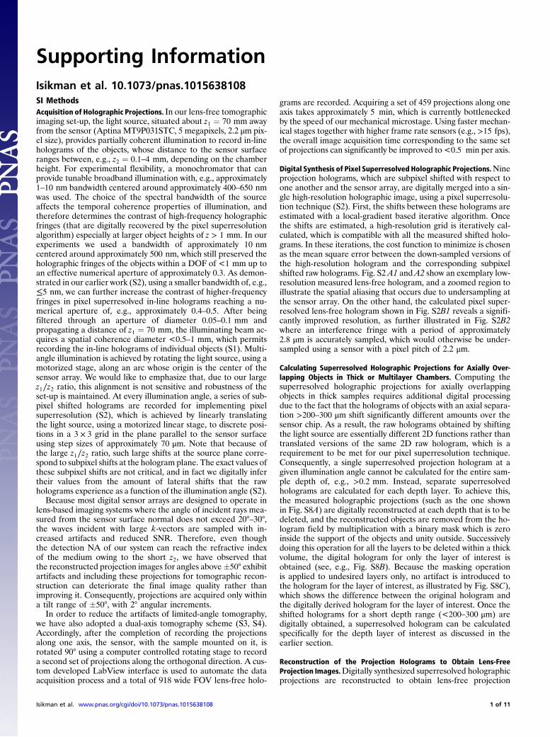
Supporting InformationIsikman et al. 10.1073/pnas.1015638108SI MethodsAcquisition of Holographic Projections. In our lens-free tomographicimaging set-up, the light source, situated about z1 ¼ 70 mm awayfrom the sensor (Aptina MT9P031STC, 5 megapixels, 2.2 μm pix-el size), provides partially coherent illumination to record in-lineholograms of the objects, whose distance to the sensor surfaceranges between, e.g., z2 ¼ 0.1–4 mm, depending on the chamberheight. For experimental flexibility, a monochromator that canprovide tunable broadband illumination with, e.g., approximately1–10 nm bandwidth centered around approximately 400–650 nmwas used. The choice of the spectral bandwidth of the sourceaffects the temporal coherence properties of illumination, andtherefore determines the contrast of high-frequency holographicfringes (that are digitally recovered by the pixel superresolutionalgorithm) especially at larger object heights of z > 1 mm. In ourexperiments we used a bandwidth of approximately 10 nmcentered around approximately 500 nm, which still preserved theholographic fringes of the objects within a DOF of <1 mm up toan effective numerical aperture of approximately 0.3. As demon-strated in our earlier work (S2), using a smaller bandwidth of, e.g.,≤5 nm, we can further increase the contrast of higher-frequencyfringes in pixel superresolved in-line holograms reaching a nu-merical aperture of, e.g., approximately 0.4–0.5. After beingfiltered through an aperture of diameter 0.05–0.1 mm andpropagating a distance of z1 ¼ 70 mm, the illuminating beam ac-quires a spatial coherence diameter <0.5–1 mm, which permitsrecording the in-line holograms of individual objects (S1). Multi-angle illumination is achieved by rotating the light source, using amotorized stage, along an arc whose origin is the center of thesensor array. We would like to emphasize that, due to our largez1∕z2 ratio, this alignment is not sensitive and robustness of theset-up is maintained. At every illumination angle, a series of sub-pixel shifted holograms are recorded for implementing pixelsuperresolution (S2), which is achieved by linearly translatingthe light source, using a motorized linear stage, to discrete posi-tions in a 3 × 3 grid in the plane parallel to the sensor surfaceusing step sizes of approximately 70 μm. Note that because ofthe large z1∕z2 ratio, such large shifts at the source plane corre-spond to subpixel shifts at the hologram plane. The exact values ofthese subpixel shifts are not critical, and in fact we digitally infertheir values from the amount of lateral shifts that the rawholograms experience as a function of the illumination angle (S2).

Because most digital sensor arrays are designed to operate inlens-based imaging systems where the angle of incident rays mea-sured from the sensor surface normal does not exceed 20°–30°,the waves incident with large k-vectors are sampled with in-creased artifacts and reduced SNR. Therefore, even thoughthe detection NA of our system can reach the refractive indexof the medium owing to the short z2, we have observed thatthe reconstructed projection images for angles above�50° exhibitartifacts and including these projections for tomographic recon-struction can deteriorate the final image quality rather thanimproving it. Consequently, projections are acquired only withina tilt range of �50°, with 2° angular increments.

In order to reduce the artifacts of limited-angle tomography,we have also adopted a dual-axis tomography scheme (S3, S4).Accordingly, after the completion of recording the projectionsalong one axis, the sensor, with the sample mounted on it, isrotated 90° using a computer controlled rotating stage to recorda second set of projections along the orthogonal direction. A cus-tom developed LabView interface is used to automate the dataacquisition process and a total of 918 wide FOV lens-free holo-

grams are recorded. Acquiring a set of 459 projections along oneaxis takes approximately 5 min, which is currently bottleneckedby the speed of our mechanical microstage. Using faster mechan-ical stages together with higher frame rate sensors (e.g., >15 fps),the overall image acquisition time corresponding to the same setof projections can significantly be improved to <0.5 min per axis.

Digital Synthesis of Pixel Superresolved Holographic Projections.Nineprojection holograms, which are subpixel shifted with respect toone another and the sensor array, are digitally merged into a sin-gle high-resolution holographic image, using a pixel superresolu-tion technique (S2). First, the shifts between these holograms areestimated with a local-gradient based iterative algorithm. Oncethe shifts are estimated, a high-resolution grid is iteratively cal-culated, which is compatible with all the measured shifted holo-grams. In these iterations, the cost function to minimize is chosenas the mean square error between the down-sampled versions ofthe high-resolution hologram and the corresponding subpixelshifted raw holograms. Fig. S2 A1 and A2 show an exemplary low-resolution measured lens-free hologram, and a zoomed region toillustrate the spatial aliasing that occurs due to undersampling atthe sensor array. On the other hand, the calculated pixel super-resolved lens-free hologram shown in Fig. S2B1 reveals a signifi-cantly improved resolution, as further illustrated in Fig. S2B2where an interference fringe with a period of approximately2.8 μm is accurately sampled, which would otherwise be under-sampled using a sensor with a pixel pitch of 2.2 μm.

Calculating Superresolved Holographic Projections for Axially Over-lapping Objects in Thick or Multilayer Chambers. Computing thesuperresolved holographic projections for axially overlappingobjects in thick samples requires additional digital processingdue to the fact that the holograms of objects with an axial separa-tion >200–300 μm shift significantly different amounts over thesensor chip. As a result, the raw holograms obtained by shiftingthe light source are essentially different 2D functions rather thantranslated versions of the same 2D raw hologram, which is arequirement to be met for our pixel superresolution technique.Consequently, a single superresolved projection hologram at agiven illumination angle cannot be calculated for the entire sam-ple depth of, e.g., >0.2 mm. Instead, separate superresolvedholograms are calculated for each depth layer. To achieve this,the measured holographic projections (such as the one shownin Fig. S8A) are digitally reconstructed at each depth that is to bedeleted, and the reconstructed objects are removed from the ho-logram field by multiplication with a binary mask which is zeroinside the support of the objects and unity outside. Successivelydoing this operation for all the layers to be deleted within a thickvolume, the digital hologram for only the layer of interest isobtained (see, e.g., Fig. S8B). Because the masking operationis applied to undesired layers only, no artifact is introduced tothe hologram for the layer of interest, as illustrated by Fig. S8C),which shows the difference between the original hologram andthe digitally derived hologram for the layer of interest. Once theshifted holograms for a short depth range (<200–300 μm) aredigitally obtained, a superresolved hologram can be calculatedspecifically for the depth layer of interest as discussed in theearlier section.

Reconstruction of the Projection Holograms to Obtain Lens-FreeProjection Images.Digitally synthesized superresolved holographicprojections are reconstructed to obtain lens-free projection

Isikman et al. www.pnas.org/cgi/doi/10.1073/pnas.1015638108 1 of 11

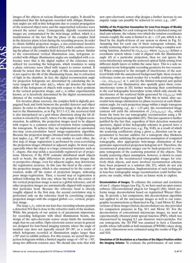
images of the objects at various illumination angles. It should beemphasized that the holograms recorded with oblique illumina-tion angles are still in-line holograms due to coaxial propagationof the scattered object wave and the unperturbed reference wavetoward the sensor array. Consequently, digitally reconstructedimages are contaminated by the twin-image artifact, which is amanifestation of the fact that the phase of the complex fieldin the detector plane is lost during the recording process. In orderto obtain faithful projection images, a size-constrained iterativephase recovery algorithm is utilized (S1), which enables recover-ing the phase of the complex field detected by the sensor. Similarto the conventional vertical illumination case, holograms re-corded with oblique illumination angles are multiplied with a re-ference wave that is the digital replica of the reference waveutilized for recording the holograms, which translates to usinga plane reference wave tilted with respect to sensor normal. Itshould be noted that the tilt angle of this reconstruction waveis not equal to the tilt of the illuminating beam, due to refractionof light in the chamber. In fact, the digital reconstruction anglefor projection holograms are determined by calculating the in-verse tangent of the ratio Δd∕z2, where Δd denotes the lateralshifts of the holograms of objects with respect to their positionsin the vertical projection image, and z2 is either experimentallyknown, or is iteratively determined by the digital reconstructiondistance of the vertical hologram.

For iterative phase recovery, the complex field is digitally pro-pagated back and forth between the parallel detector and objectplanes. In order to obtain the projection image in the plane nor-mal to the illumination, as in Fig. S3 C1–C3, the recovered fieldis also interpolated on a grid whose dimension along the tilt di-rection is rescaled by cosðθÞ, where θ is the angle of digital recon-struction. In addition, the projection images need to be alignedwith respect to a common center-of-rotation before computingthe tomograms. To achieve that, we implemented an automatedtwo-step cross-correlation based image-registration algorithm.Because the projection images obtained with successive illumina-tion angles, e.g., 50° and 48°, are very similar to each other, thefirst step of image registration is performed by cross-correlatingthe projection images obtained at adjacent angles. In most cases,especially when the object is a large connected structure such asC. elegans, this step yields a successfully registered set of projec-tions. However, if the FOV contains distributed small objectssuch as beads, the slight differences in projection images dueto perspective change, even for adjacent angles, may deterioratethe registration accuracy. In this case the bead at the center ofthe projection images, which is also assumed to be the center ofrotation, walks off the center of projection images, indicatingpoor image-registration. Then, a second step of registration isutilized following the first one, where the bead at the center ofthe vertical projection image is used as a global reference, and allother projection images are automatically aligned with respect tothat particular bead. Because the reference bead is alreadyroughly aligned in the first step, the second correlation step isperformed only on the reference bead by correlating croppedprojection images with the cropped global—i.e., vertical, projec-tion image.

The large z1∕z2 ratio in our lens-free recording scheme permitsa detection NA that is close to the refractive index of the medium.While this property of our system is of paramount importancefor recording holograms with tilted illumination beams, thedesign of the opto-electronic sensor arrays limits the maximumangle that we can utilize. Opto-electronic sensor arrays in generalare designed for lens-based imaging systems, where the angle ofincident rays does not typically exceed 20°–30°, as a result ofwhich holograms recorded at illumination angles larger than�50° start to exhibit artifacts. For this reason, we record the pro-jection holograms within a limited angular range of −50° toþ50°,along two different rotation axes. We should also note that with

new opto-electronic sensor chip designs a further increase in ourangular range can possibly be achieved to cover, e.g., �80°.

Validity of the Projection Assumption for Lens-Free Images of WeaklyScattering Objects. For each tomogram that is calculated using ourdual-axis scheme, the volume over which the rotation coordinatesremain roughly the same is limited to Δz ∼�25 μm, which is de-fined by the depth-of-focus of our system as shown in Fig. S1.Assuming that for each one of these tomogram volumes, theweakly scattering object can be represented using a complex scat-tering function, denoted by sðxθ;yθ;zθÞ, where ðxθ;yθ;zθÞ defines acoordinate system whose z-axis is aligned with the illuminationangle (θ) at a particular projection, then we can ignore thecross-interference among the scattered optical fields arising fromdifferent depth layers or within the same layer. This is a safe as-sumption in our holographic recording geometry for two reasons:(i) When compared to the strength of interference of the scat-tered fields with the unscattered background light, these cross-in-terference terms are much weaker for a weakly scattering object—i.e., jsðxθ;yθ;zθÞj ≪ 1; and (ii) the limited temporal and spatialcoherence of our illumination also spatially gates these cross-interference terms in 3D, further weakening their contributionto the real holographic heterodyne terms which only encode theinterference of the scattered fields generated by sðxθ;yθ;zθÞ withthe unscattered background light. With this in mind, after suc-cessful twin-image elimination (or phase recovery) at each illumi-nation angle, for each projection image within a single tomogramvolume (spanning, e.g., Δz ∼�25 μm), the reconstructed imagecontrast will yield the information of ∫ jsðxθ;yθ;zθÞj · dzθ, whichforms the basis for our tomographic reconstruction using a fil-tered back-projection algorithm (S5). This last equation is furtherjustified by the fact that, regardless of their detection numericalapertures, digital in-line holography schemes in general have avery long depth of focus (see, e.g., Fig. S1B), as a result of whichthe scattering coefficients along a given zθ direction can be ap-proximated to become additive for a tomogram slice thicknessof Δz ∼ 50 μm, satisfying the projection assumption of computedtomography, after appropriate twin-image elimination of thatparticular superresolved projection hologram at θ. Therefore, thereconstructed projection images can be back-projected to com-pute tomograms of the scattering potential of the objects. Thisweakly scattering object assumption, however, is shown to causeaberrations in the reconstructed tomographic images for rela-tively thick objects, and more involved reconstruction schemeshave been proposed as a solution (S6, S7), which do not relyon the Born approximation. Implementation of such techniquesin lens-free tomographic image reconstruction could further im-prove our results, which we leave as future work to explore.

Deconvolution of Images. To enhance the contrast and resolutionof our C. elegans images (see Fig. 3), we have used an open sourcesoftware (DeconvolutionJ plug-in for ImageJ) (S8), which per-forms image deconvolution based on regularized Wiener filter-ing. To provide a fair comparison, this deconvolution algorithmwas applied to all the microscope images as well to our tomo-graphic reconstructions as illustrated in Fig. 3 and Movie S2. Rawversions of these images (before deconvolution) are also providedfor comparison purposes in Fig. S11 and Movie S3. For thedeconvolution of conventional microscope images, we used anexperimentally obtained point spread function (PSF), which wascharacterized by imaging 0.2 μm diameter micro-particles. Forour tomograms, the 3D PSF was assumed to have a Gaussianprofile whose full-width-at-half-maximum (FWHM) values alongx, y, and z dimensions were estimated using the results of Figs. S9and S10.

Simulation of 3D Resolution as a Function of the Object Position withinthe Imaging Volume. To evaluate the performance of our tomo-

Isikman et al. www.pnas.org/cgi/doi/10.1073/pnas.1015638108 2 of 11

graphic on-chip microscope and its dependence on the objectposition within our imaging volume, we conducted a numericalsimulation, whose results are shown in Fig. S10. In this simula-tion, we computed the tomograms of an object (opaque sphericalparticle with 4 μm diameter) located at different points within ourlarge imaging volume. To account for the effect of change in ob-ject’s vertical position over the sensor, this opaque micro-objectwas placed at four different depths between z ¼ 0.7 mm andz ¼ 3.8 mm, and vertical in-line holograms of the particle wereexperimentally acquired at each depth using the set-up shownin Fig. S1. These experimentally obtained vertical projectionimages (after holographic reconstruction) were then duplicatedto serve as the projection images for all the possible viewing an-gles corresponding to any given object position within the imagingvolume. In order to incorporate the effect of lateral position ofthe objects on resolution, the number of projection images uti-lized to compute tomograms was varied, as determined by theangular range for which projection holograms of the object couldbe recorded without its hologram shifting out of the field of view(determined by the physical sensor size—i.e., 24 mm2). Forinstance, to simulate the case where the particle is located at,e.g., z ¼ 3 mm, x ¼ −2.8 mm and y ¼ 0 mm (such that the par-ticle is located at the center of the short edge of the sensor field ofview), for the first axial scan (along x) we only used 26 projectionimages corresponding to an angular range of 0° to 50° (as opposedto �50° for the best case), and for the second orthogonal scan(along y), we only used 45 projections corresponding to an angu-lar range of�44° (as opposed to�50° for the best case). Based onthis scheme, a good estimate for experimentally achievable reso-lution can be obtained by calculating the FWHM of the spatialderivative of the edge response (as described in refs. S9–S11) inthese computed tomograms as a function of the position of the

particle. In these simulations, possible aberrations in the projec-tion images reconstructed at large angles are neglected since wehave used the experimentally obtained vertical projection imagesfor all the angles. Nevertheless, with this simulation scheme, thechange in digital signal-to-noise ratio (SNR) of the holograms asa function of object depth (z) is taken into account as well as thereduction in available viewing angles as a function of the lateralposition ðx;yÞ of the objects. Therefore, the results of this simula-tion, presented in Fig. S10, give a realistic upper limit for theposition dependent spatial resolution that can be achieved withour lens-free tomographic on-chip microscope. The fact that theexperimentally achieved results shown Fig. S9 closely follow oursimulation results further supports the validity of our assumptionsmade in this simulation.

In our imaging geometry shown in Fig. 1, the entire angularrange of �50° can be utilized over an FOV of approximately15 mm2 and up to a DOF of approximately 1 mm. As a result,a spatial resolution of <1 μm× < 1 μm× < 3 μm in x, y, and zdimensions, respectively, can be achieved over an imaging volumeof approximately 15 mm3, without a significant change in recon-structed image quality as also indicated by Figs. S9 and S10. Notealso that by increasing the DOF up to approximately 2–4 mm,and using an FOVof approximately 24 mm2 (the total active areaof the sensor), this imaging volume can be further increased to48–96 mm3 at the cost of reduced spatial resolution (i.e., approxi-mately 3–6 μm axial, approximately 1.2–1.8 μm lateral), which ismainly due to reduced signal-to-noise ratio (SNR) of lens-freeholograms acquired at larger depth values of >1 mm, as wellas a reduced number of angles available for back-projection forregions outside the 15 mm3 sample volume that offers the bestresolution.

1. Mudanyali O, et al. (2010) Compact, light-weight and cost-effective microscopebased on lensless incoherent holography for telemedicine applications. Lab Chip10:1417–1428.

2. Bishara W, Su T, Coskun AF, and Ozcan A (2010) Lensfree on-chip microscopy over awide field-of-view using pixel super-resolution. Opt Express 18:11181–11191.

3. Mastronarde DN (1997) Dual-axis tomography: An approach with alignment methodsthat preserve resolution. J Struct Biol 120:343–352.

4. Arslan I, Tong JR,Midgley PA (2006) Reducing themissingwedge: High-resolution dualaxis tomography of inorganic materials. Ultramicroscopy 106:994–1000.

5. Radermacher M (2006) Weighted Back-Projection Methods. Electron Tomography:Methods for Three Dimensional Visualization of Structures in the Cell, 2nd Ed. (Spring-er, New York) pp 245–273.

6. Sung Y, et al. (2008) Optical diffraction tomography for high resolution live cellimaging. Opt Express 17:266–277.

7. MalekiMH, Devaney AJ, SchatzbergA (1992) Tomographic reconstruction from opticalscattered intensities. J Opt Soc Am A 9:1356–1363.

8. Abramoff MD, Magelhaes P, Ram SJ (2004) Image processing with ImageJ. Biopho-tonics International 11:36–42.

9. Choi W, et al. (2007) Tomographic phase microscopy. Nat Methods 4:717–719.10. Sung Y, et al. (2008) Optical diffraction tomography for high resolution live cell

imaging. Opt Express 17:266–277.11. Oh WY, Bouma BE, Iftimia N, Yelin R, Tearney GJ (2006) Spectrally-modulated full-

field optical coherence microscopy for ultrahigh-resolution endoscopic imaging.Opt Express 18:8675–8684.

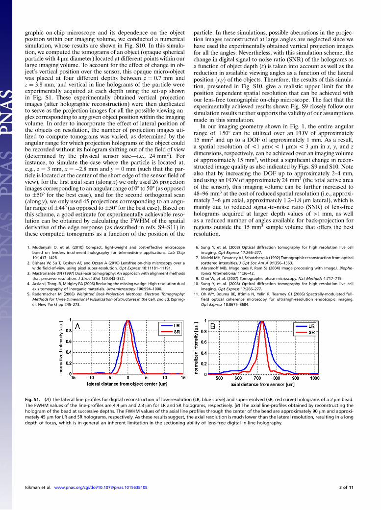
Fig. S1. (A) The lateral line profiles for digital reconstruction of low-resolution (LR, blue curve) and superresolved (SR, red curve) holograms of a 2 μm bead.The FWHM values of the line-profiles are 4.4 μm and 2.8 μm for LR and SR holograms, respectively. (B) The axial line-profiles obtained by reconstructing thehologram of the bead at successive depths. The FWHM values of the axial line profiles through the center of the bead are approximately 90 μm and approxi-mately 45 μm for LR and SR holograms, respectively. As these results suggest, the axial resolution is much lower than the lateral resolution, resulting in a longdepth of focus, which is in general an inherent limitation in the sectioning ability of lens-free digital in-line holography.

Isikman et al. www.pnas.org/cgi/doi/10.1073/pnas.1015638108 3 of 11

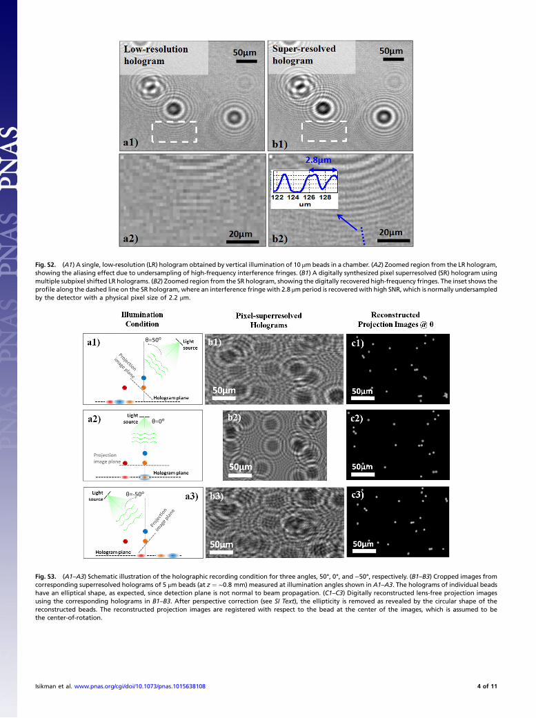
Fig. S2. (A1) A single, low-resolution (LR) hologram obtained by vertical illumination of 10 μmbeads in a chamber. (A2) Zoomed region from the LR hologram,showing the aliasing effect due to undersampling of high-frequency interference fringes. (B1) A digitally synthesized pixel superresolved (SR) hologram usingmultiple subpixel shifted LR holograms. (B2) Zoomed region from the SR hologram, showing the digitally recovered high-frequency fringes. The inset shows theprofile along the dashed line on the SR hologram, where an interference fringe with 2.8 μmperiod is recovered with high SNR, which is normally undersampledby the detector with a physical pixel size of 2.2 μm.

Fig. S3. (A1–A3) Schematic illustration of the holographic recording condition for three angles, 50°, 0°, and −50°, respectively. (B1–B3) Cropped images fromcorresponding superresolved holograms of 5 μm beads (at z ¼ ∼0.8 mm) measured at illumination angles shown in A1–A3. The holograms of individual beadshave an elliptical shape, as expected, since detection plane is not normal to beam propagation. (C1–C3) Digitally reconstructed lens-free projection imagesusing the corresponding holograms in B1–B3. After perspective correction (see SI Text), the ellipticity is removed as revealed by the circular shape of thereconstructed beads. The reconstructed projection images are registered with respect to the bead at the center of the images, which is assumed to bethe center-of-rotation.

Isikman et al. www.pnas.org/cgi/doi/10.1073/pnas.1015638108 4 of 11

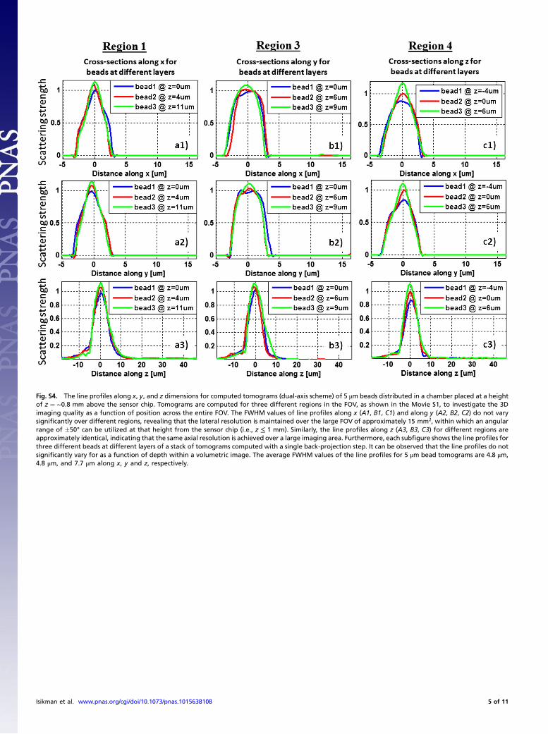
Fig. S4. The line profiles along x, y, and z dimensions for computed tomograms (dual-axis scheme) of 5 μm beads distributed in a chamber placed at a heightof z ¼ ∼0.8 mm above the sensor chip. Tomograms are computed for three different regions in the FOV, as shown in the Movie S1, to investigate the 3Dimaging quality as a function of position across the entire FOV. The FWHM values of line profiles along x (A1, B1, C1) and along y (A2, B2, C2) do not varysignificantly over different regions, revealing that the lateral resolution is maintained over the large FOV of approximately 15 mm2, within which an angularrange of �50° can be utilized at that height from the sensor chip (i.e., z ≤ 1 mm). Similarly, the line profiles along z (A3, B3, C3) for different regions areapproximately identical, indicating that the same axial resolution is achieved over a large imaging area. Furthermore, each subfigure shows the line profiles forthree different beads at different layers of a stack of tomograms computed with a single back-projection step. It can be observed that the line profiles do notsignificantly vary for as a function of depth within a volumetric image. The average FWHM values of the line profiles for 5 μm bead tomograms are 4.8 μm,4.8 μm, and 7.7 μm along x, y and z, respectively.

Isikman et al. www.pnas.org/cgi/doi/10.1073/pnas.1015638108 5 of 11

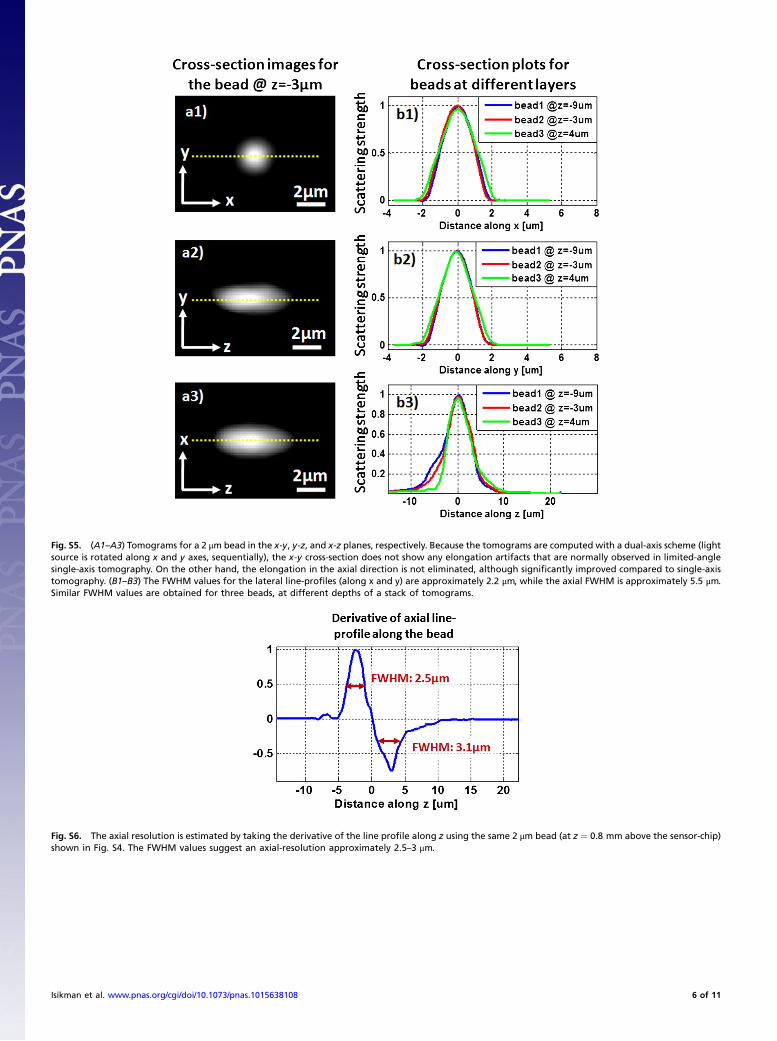
Fig. S5. (A1–A3) Tomograms for a 2 μm bead in the x-y, y-z, and x-z planes, respectively. Because the tomograms are computed with a dual-axis scheme (lightsource is rotated along x and y axes, sequentially), the x-y cross-section does not show any elongation artifacts that are normally observed in limited-anglesingle-axis tomography. On the other hand, the elongation in the axial direction is not eliminated, although significantly improved compared to single-axistomography. (B1–B3) The FWHM values for the lateral line-profiles (along x and y) are approximately 2.2 μm, while the axial FWHM is approximately 5.5 μm.Similar FWHM values are obtained for three beads, at different depths of a stack of tomograms.

Fig. S6. The axial resolution is estimated by taking the derivative of the line profile along z using the same 2 μm bead (at z ¼ 0.8 mm above the sensor-chip)shown in Fig. S4. The FWHM values suggest an axial-resolution approximately 2.5–3 μm.

Isikman et al. www.pnas.org/cgi/doi/10.1073/pnas.1015638108 6 of 11

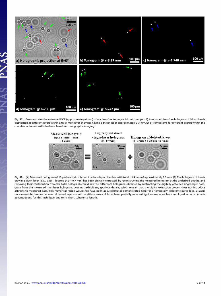
Fig. S7. Demonstrates the extended DOF (approximately 4 mm) of our lens-free tomographic microscope. (A) A recorded lens-free hologram of 10 μm beadsdistributed at different layers within a thick multilayer chamber having a thickness of approximately 3.3 mm. (B–E) Tomograms for different depths within thechamber obtained with dual-axis lens-free tomographic imaging.

Fig. S8. (A) Measured hologram of 10 μm beads distributed in a four-layer chamber with total thickness of approximately 3.3 mm. (B) The hologram of beadsonly in a given layer (e.g., layer 1 located at z ∼ 0.7 mm) has been digitally extracted, by reconstructing the measured hologram at the undesired depths, andremoving their contribution from the total holographic field. (C) The difference hologram, obtained by subtracting the digitally obtained single-layer holo-gram from the measured multilayer hologram, does not exhibit any spurious details, which reveals that the digital extraction process does not introduceartifacts to measured data. This numerical recipe would not have been as successful as demonstrated here for a temporally coherent source (e.g., a laser)since cross-interference between different layers would constitute errors. A broadband partially coherent light source as we have employed in our scheme isadvantageous for this technique due to its short coherence length.

Isikman et al. www.pnas.org/cgi/doi/10.1073/pnas.1015638108 7 of 11

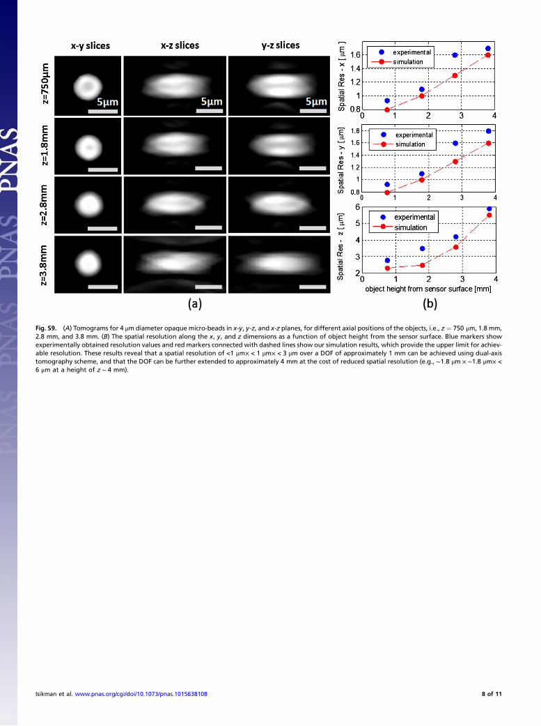
Fig. S9. (A) Tomograms for 4 μm diameter opaque micro-beads in x-y, y-z, and x-z planes, for different axial positions of the objects, i.e., z ¼ 750 μm, 1.8 mm,2.8 mm, and 3.8 mm. (B) The spatial resolution along the x, y, and z dimensions as a function of object height from the sensor surface. Blue markers showexperimentally obtained resolution values and red markers connected with dashed lines show our simulation results, which provide the upper limit for achiev-able resolution. These results reveal that a spatial resolution of <1 μm× < 1 μm× < 3 μm over a DOF of approximately 1 mm can be achieved using dual-axistomography scheme, and that the DOF can be further extended to approximately 4 mm at the cost of reduced spatial resolution (e.g., ∼1.8 μm × ∼1.8 μm× <6 μm at a height of z ∼ 4 mm).

Isikman et al. www.pnas.org/cgi/doi/10.1073/pnas.1015638108 8 of 11

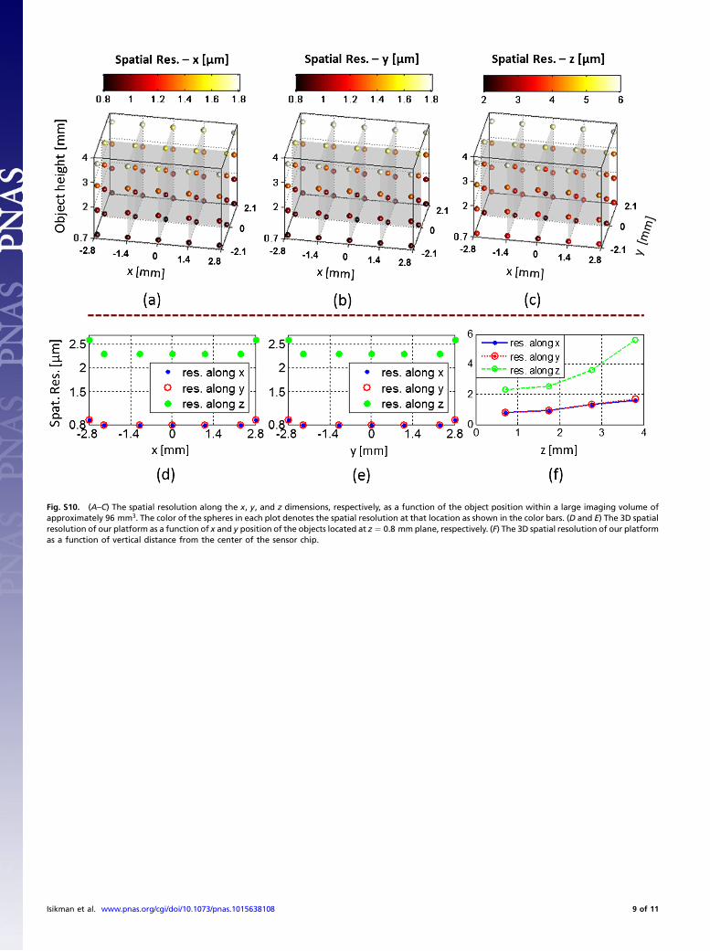
Fig. S10. (A–C) The spatial resolution along the x, y, and z dimensions, respectively, as a function of the object position within a large imaging volume ofapproximately 96 mm3. The color of the spheres in each plot denotes the spatial resolution at that location as shown in the color bars. (D and E) The 3D spatialresolution of our platform as a function of x and y position of the objects located at z ¼ 0.8 mmplane, respectively. (F) The 3D spatial resolution of our platformas a function of vertical distance from the center of the sensor chip.

Isikman et al. www.pnas.org/cgi/doi/10.1073/pnas.1015638108 9 of 11

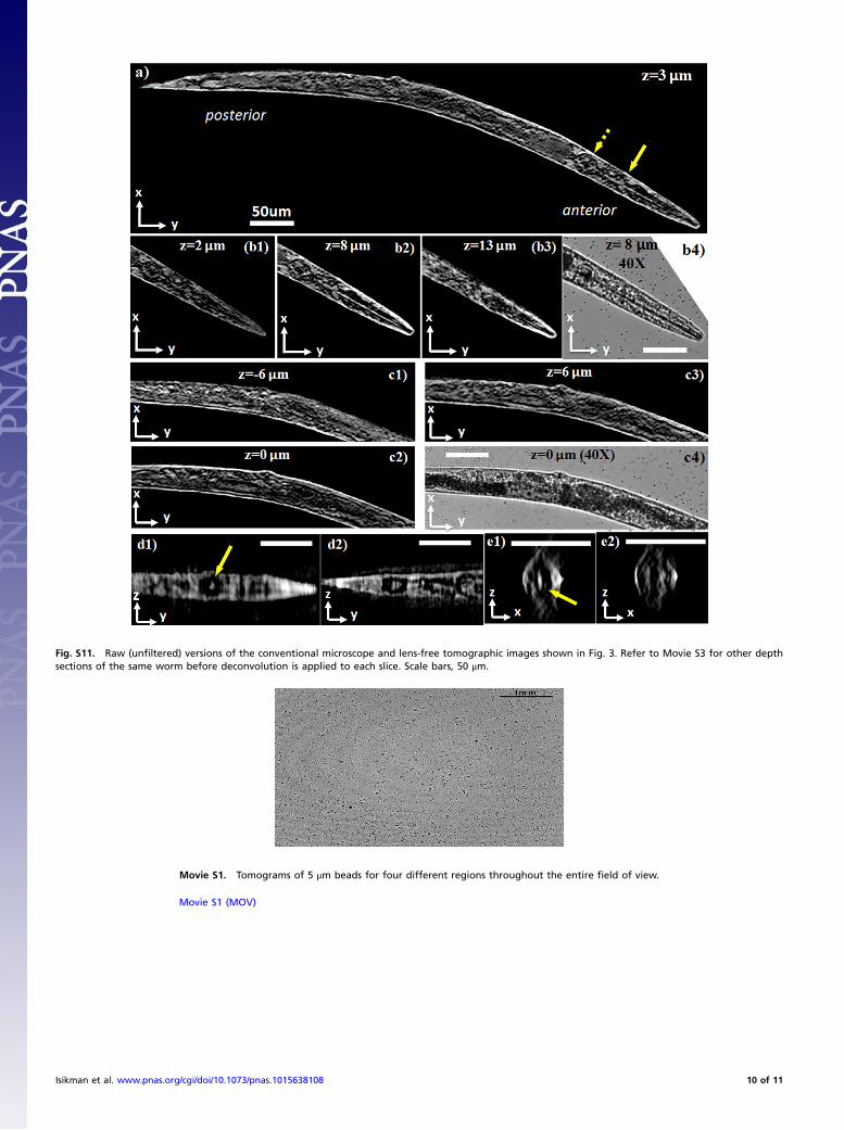
Fig. S11. Raw (unfiltered) versions of the conventional microscope and lens-free tomographic images shown in Fig. 3. Refer to Movie S3 for other depthsections of the same worm before deconvolution is applied to each slice. Scale bars, 50 μm.

Movie S1. Tomograms of 5 μm beads for four different regions throughout the entire field of view.

Movie S1 (MOV)

Isikman et al. www.pnas.org/cgi/doi/10.1073/pnas.1015638108 10 of 11

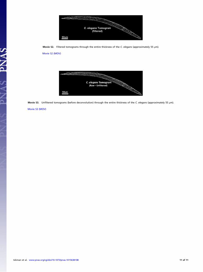
Movie S2. Filtered tomograms through the entire thickness of the C. elegans (approximately 55 μm).

Movie S2 (MOV)

Movie S3. Unfiltered tomograms (before deconvolution) through the entire thickness of the C. elegans (approximately 55 μm).

Movie S3 (MOV)

Isikman et al. www.pnas.org/cgi/doi/10.1073/pnas.1015638108 11 of 11