Supplementary material for the manuscript - ACP - Recent · 2016-01-11 · 3 29 30 Table S 3:...
22
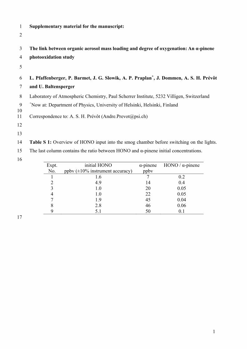
1 Supplementary material for the manuscript: 1 2 The link between organic aerosol mass loading and degree of oxygenation: An α-pinene 3 photooxidation study 4 5 L. Pfaffenberger, P. Barmet, J. G. Slowik, A. P. Praplan + , J. Dommen, A. S. H. Prévôt 6 and U. Baltensperger 7 Laboratory of Atmospheric Chemistry, Paul Scherrer Institute, 5232 Villigen, Switzerland 8 + Now at: Department of Physics, University of Helsinki, Helsinki, Finland 9 10 Correspondence to: A. S. H. Prévôt ([email protected]) 11 12 13 Table S 1: Overview of HONO input into the smog chamber before switching on the lights. 14 The last column contains the ratio between HONO and α-pinene initial concentrations. 15 16 Expt. initial HONO α-pinene HONO / α-pinene No. ppbv (±10% instrument accuracy) ppbv 1 1.6 7 0.2 2 4.9 14 0.4 3 1.0 20 0.05 4 1.0 22 0.05 7 1.9 45 0.04 8 2.8 46 0.06 9 5.1 50 0.1 17
Transcript of Supplementary material for the manuscript - ACP - Recent · 2016-01-11 · 3 29 30 Table S 3:...
1
Supplementary material for the manuscript: 1
2
The link between organic aerosol mass loading and degree of oxygenation: An α-pinene 3
photooxidation study 4
5
L. Pfaffenberger, P. Barmet, J. G. Slowik, A. P. Praplan+, J. Dommen, A. S. H. Prévôt 6
and U. Baltensperger 7
Laboratory of Atmospheric Chemistry, Paul Scherrer Institute, 5232 Villigen, Switzerland 8 +Now at: Department of Physics, University of Helsinki, Helsinki, Finland 9 10 Correspondence to: A. S. H. Prévôt ([email protected]) 11
12
13
Table S 1: Overview of HONO input into the smog chamber before switching on the lights. 14
The last column contains the ratio between HONO and α-pinene initial concentrations. 15
16 Expt. initial HONO α-pinene HONO / α-pinene No. ppbv (±10% instrument accuracy) ppbv 1 1.6 7 0.2 2 4.9 14 0.4 3 1.0 20 0.05 4 1.0 22 0.05 7 1.9 45 0.04 8 2.8 46 0.06 9 5.1 50 0.1
17
2
18
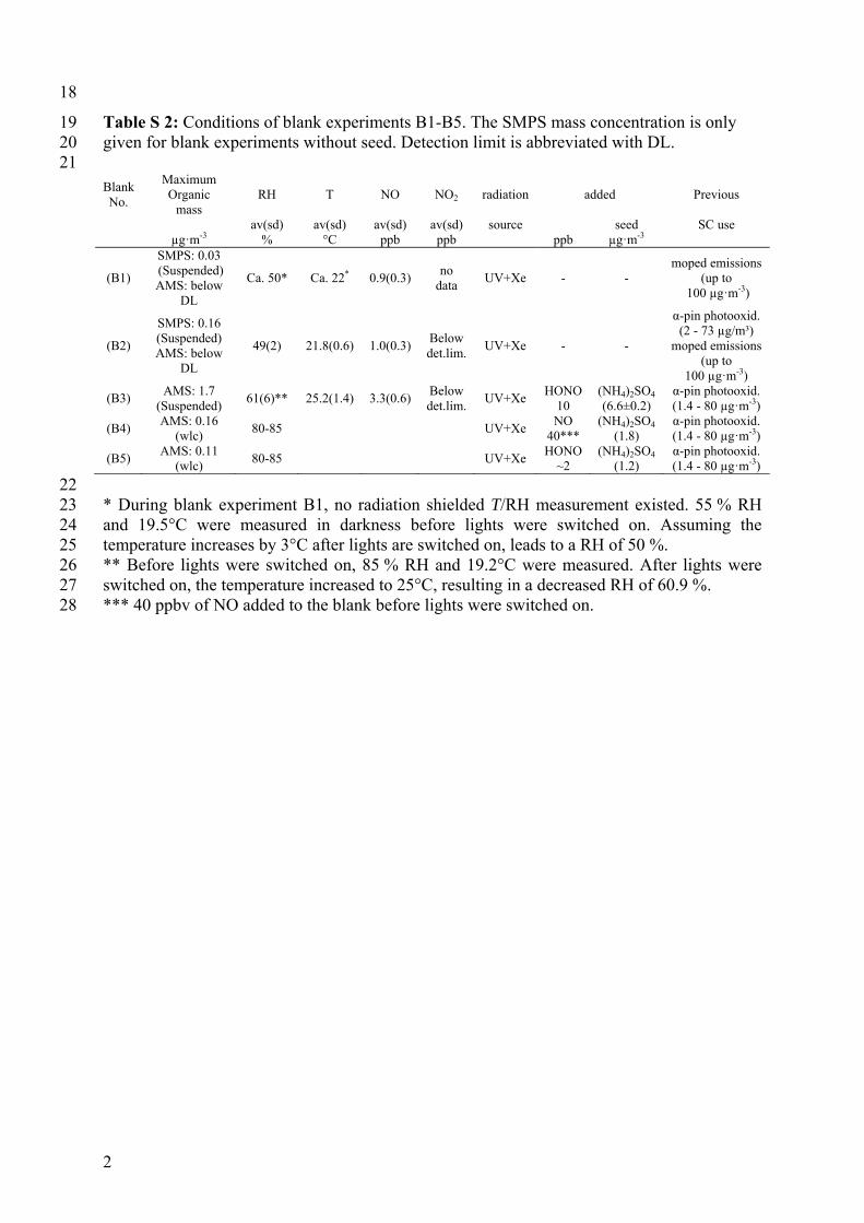
Table S 2: Conditions of blank experiments B1-B5. The SMPS mass concentration is only 19 given for blank experiments without seed. Detection limit is abbreviated with DL. 20 21 Blank No.
Maximum Organic
mass RH T NO NO2 radiation added Previous
av(sd) av(sd) av(sd) av(sd) source seed SC use µg·m-3 % °C ppb ppb ppb µg·m-3
(B1)
SMPS: 0.03 (Suspended) AMS: below
DL
Ca. 50* Ca. 22* 0.9(0.3) no
data UV+Xe - -
moped emissions (up to
100 µg·m-3)
(B2)
SMPS: 0.16 (Suspended) AMS: below
DL
49(2) 21.8(0.6) 1.0(0.3) Below det.lim.
UV+Xe - -
α-pin photooxid. (2 - 73 µg/m³)
moped emissions (up to
100 µg·m-3)
(B3) AMS: 1.7
(Suspended) 61(6)** 25.2(1.4) 3.3(0.6)
Below det.lim.
UV+Xe HONO
10 (NH4)2SO4 (6.6±0.2)
α-pin photooxid. (1.4 - 80 µg·m-3)
(B4) AMS: 0.16
(wlc) 80-85 UV+Xe
NO 40***
(NH4)2SO4 (1.8)
α-pin photooxid. (1.4 - 80 µg·m-3)
(B5) AMS: 0.11
(wlc) 80-85 UV+Xe
HONO ~2
(NH4)2SO4 (1.2)
α-pin photooxid. (1.4 - 80 µg·m-3)
22 * During blank experiment B1, no radiation shielded T/RH measurement existed. 55 % RH 23 and 19.5°C were measured in darkness before lights were switched on. Assuming the 24 temperature increases by 3°C after lights are switched on, leads to a RH of 50 %. 25 ** Before lights were switched on, 85 % RH and 19.2°C were measured. After lights were 26 switched on, the temperature increased to 25°C, resulting in a decreased RH of 60.9 %. 27 *** 40 ppbv of NO added to the blank before lights were switched on. 28
3
29
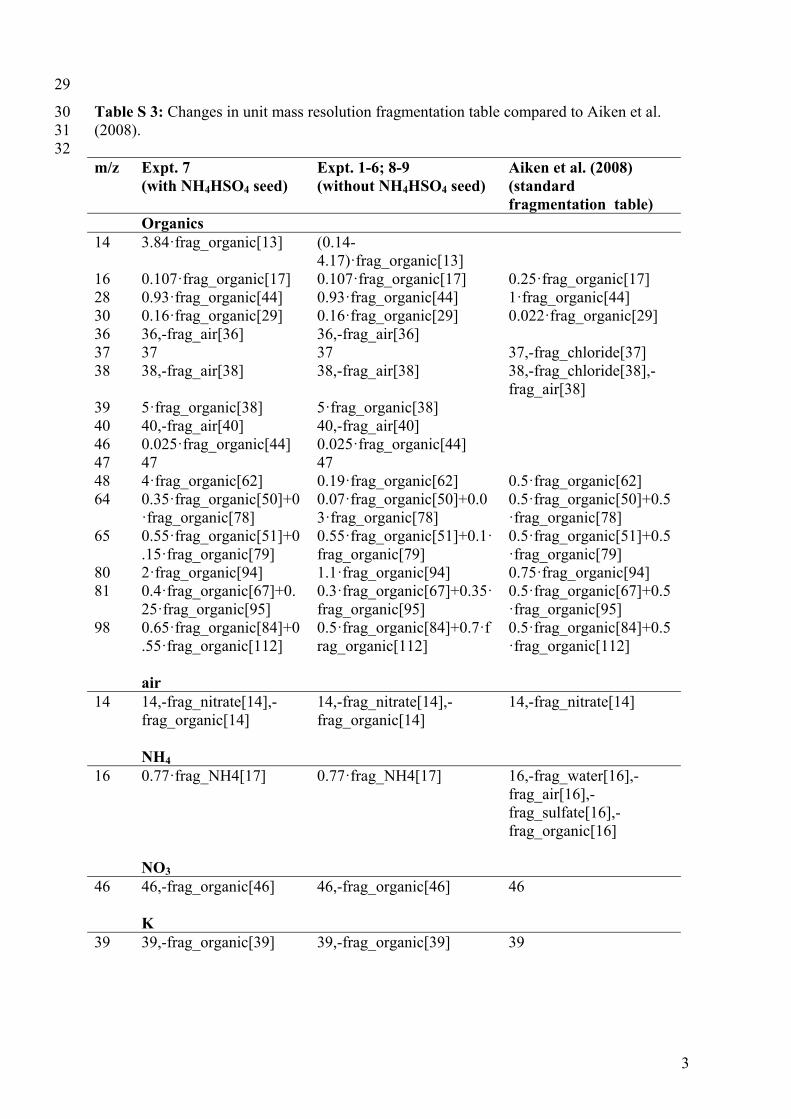
Table S 3: Changes in unit mass resolution fragmentation table compared to Aiken et al. 30 (2008). 31 32 m/z Expt. 7
(with NH4HSO4 seed) Expt. 1-6; 8-9 (without NH4HSO4 seed)
Aiken et al. (2008) (standard fragmentation table)
Organics 14 3.84·frag_organic[13] (0.14-
4.17)·frag_organic[13]
16 0.107·frag_organic[17] 0.107·frag_organic[17] 0.25·frag_organic[17] 28 0.93·frag_organic[44] 0.93·frag_organic[44] 1·frag_organic[44] 30 0.16·frag_organic[29] 0.16·frag_organic[29] 0.022·frag_organic[29] 36 36,-frag_air[36] 36,-frag_air[36] 37 37 37 37,-frag_chloride[37] 38 38,-frag_air[38] 38,-frag_air[38] 38,-frag_chloride[38],-
frag_air[38] 39 5·frag_organic[38] 5·frag_organic[38] 40 40,-frag_air[40] 40,-frag_air[40] 46 0.025·frag_organic[44] 0.025·frag_organic[44] 47 47 47 48 4·frag_organic[62] 0.19·frag_organic[62] 0.5·frag_organic[62] 64 0.35·frag_organic[50]+0
·frag_organic[78] 0.07·frag_organic[50]+0.03·frag_organic[78]
0.5·frag_organic[50]+0.5·frag_organic[78]
65 0.55·frag_organic[51]+0.15·frag_organic[79]
0.55·frag_organic[51]+0.1·frag_organic[79]
0.5·frag_organic[51]+0.5·frag_organic[79]
80 2·frag_organic[94] 1.1·frag_organic[94] 0.75·frag_organic[94] 81 0.4·frag_organic[67]+0.
25·frag_organic[95] 0.3·frag_organic[67]+0.35·frag_organic[95]
0.5·frag_organic[67]+0.5·frag_organic[95]
98 0.65·frag_organic[84]+0.55·frag_organic[112]
0.5·frag_organic[84]+0.7·frag_organic[112]
0.5·frag_organic[84]+0.5·frag_organic[112]
air 14 14,-frag_nitrate[14],-
frag_organic[14] 14,-frag_nitrate[14],-frag_organic[14]
14,-frag_nitrate[14]
NH4 16 0.77·frag_NH4[17] 0.77·frag_NH4[17] 16,-frag_water[16],-
frag_air[16],-frag_sulfate[16],-frag_organic[16]
NO3 46 46,-frag_organic[46] 46,-frag_organic[46] 46 K 39 39,-frag_organic[39] 39,-frag_organic[39] 39
4
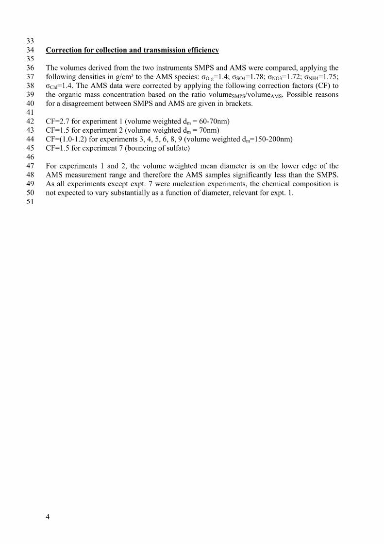
33 Correction for collection and transmission efficiency 34 35 The volumes derived from the two instruments SMPS and AMS were compared, applying the 36 following densities in g/cm³ to the AMS species: σOrg=1.4; σSO4=1.78; σNO3=1.72; σNH4=1.75; 37 σChl=1.4. The AMS data were corrected by applying the following correction factors (CF) to 38 the organic mass concentration based on the ratio volumeSMPS/volumeAMS. Possible reasons 39 for a disagreement between SMPS and AMS are given in brackets. 40 41 CF=2.7 for experiment 1 (volume weighted dm = 60-70nm) 42 CF=1.5 for experiment 2 (volume weighted dm = 70nm) 43 CF=(1.0-1.2) for experiments 3, 4, 5, 6, 8, 9 (volume weighted dm=150-200nm) 44 CF=1.5 for experiment 7 (bouncing of sulfate) 45 46 For experiments 1 and 2, the volume weighted mean diameter is on the lower edge of the 47 AMS measurement range and therefore the AMS samples significantly less than the SMPS. 48 As all experiments except expt. 7 were nucleation experiments, the chemical composition is 49 not expected to vary substantially as a function of diameter, relevant for expt. 1. 50 51
5
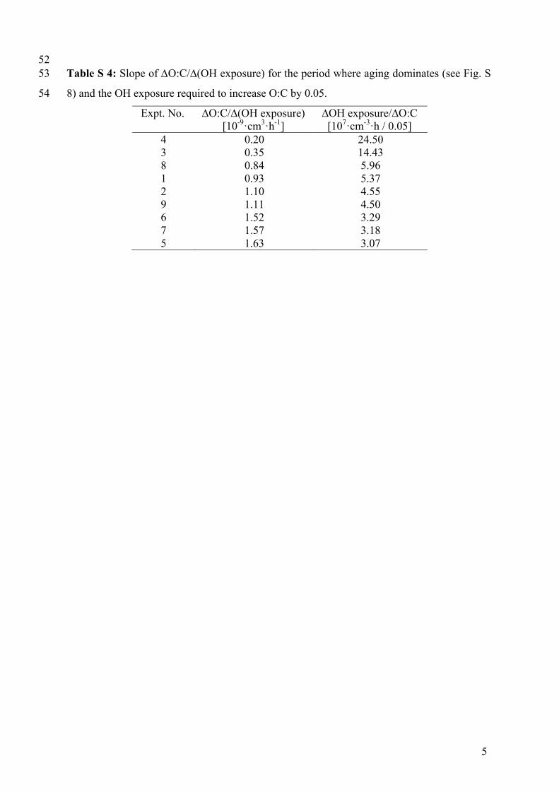
52 Table S 4: Slope of O:C/∆(OH exposure) for the period where aging dominates (see Fig. S 53
8) and the OH exposure required to increase O:C by 0.05. 54
Expt. No. ∆O:C/∆(OH exposure) ∆OH exposure/∆O:C [10-9·cm3·h-1] [107·cm-3·h / 0.05] 4 0.20 24.50 3 0.35 14.43 8 0.84 5.96 1 0.93 5.37 2 1.10 4.55 9 1.11 4.50 6 1.52 3.29 7 1.57 3.18 5 1.63 3.07
6
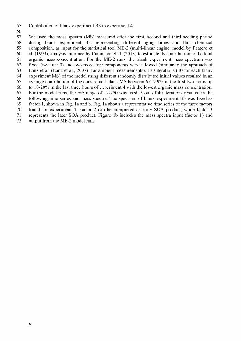
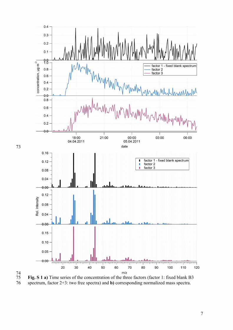
Contribution of blank experiment B3 to experiment 4 55 56 We used the mass spectra (MS) measured after the first, second and third seeding period 57 during blank experiment B3, representing different aging times and thus chemical 58 composition, as input for the statistical tool ME-2 (multi-linear engine: model by Paatero et 59 al. (1999), analysis interface by Canonaco et al. (2013) to estimate its contribution to the total 60 organic mass concentration. For the ME-2 runs, the blank experiment mass spectrum was 61 fixed (a-value: 0) and two more free components were allowed (similar to the approach of 62 Lanz et al. (Lanz et al., 2007) for ambient measurements). 120 iterations (40 for each blank 63 experiment MS) of the model using different randomly distributed initial values resulted in an 64 average contribution of the constrained blank MS between 6.6-9.9% in the first two hours up 65 to 10-20% in the last three hours of experiment 4 with the lowest organic mass concentration. 66 For the model runs, the m/z range of 12-250 was used. 5 out of 40 iterations resulted in the 67 following time series and mass spectra. The spectrum of blank experiment B3 was fixed as 68 factor 1, shown in Fig. 1a and b. Fig. 1a shows a representative time series of the three factors 69 found for experiment 4. Factor 2 can be interpreted as early SOA product, while factor 3 70 represents the later SOA product. Figure 1b includes the mass spectra input (factor 1) and 71 output from the ME-2 model runs. 72
7
73
74 Fig. S 1 a) Time series of the concentration of the three factors (factor 1: fixed blank B3 75 spectrum, factor 2+3: two free spectra) and b) corresponding normalized mass spectra. 76
8
77
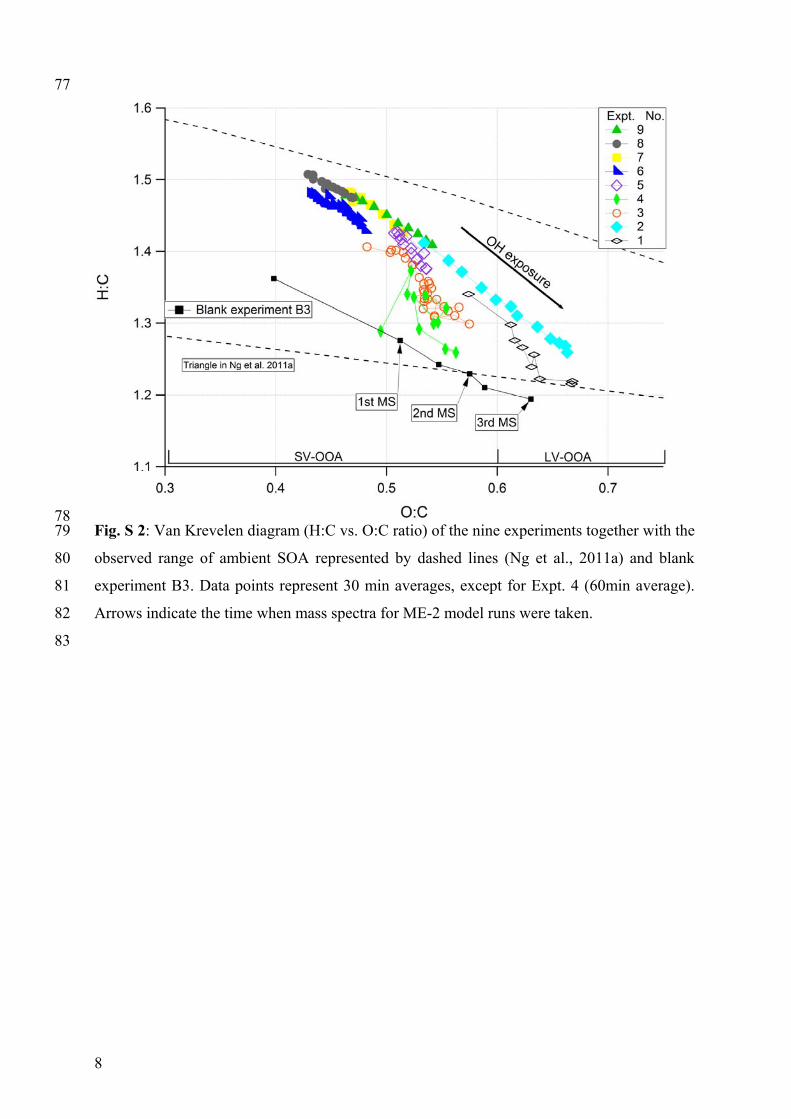
78 Fig. S 2: Van Krevelen diagram (H:C vs. O:C ratio) of the nine experiments together with the 79
observed range of ambient SOA represented by dashed lines (Ng et al., 2011a) and blank 80
experiment B3. Data points represent 30 min averages, except for Expt. 4 (60min average). 81
Arrows indicate the time when mass spectra for ME-2 model runs were taken. 82
83
9
84
85
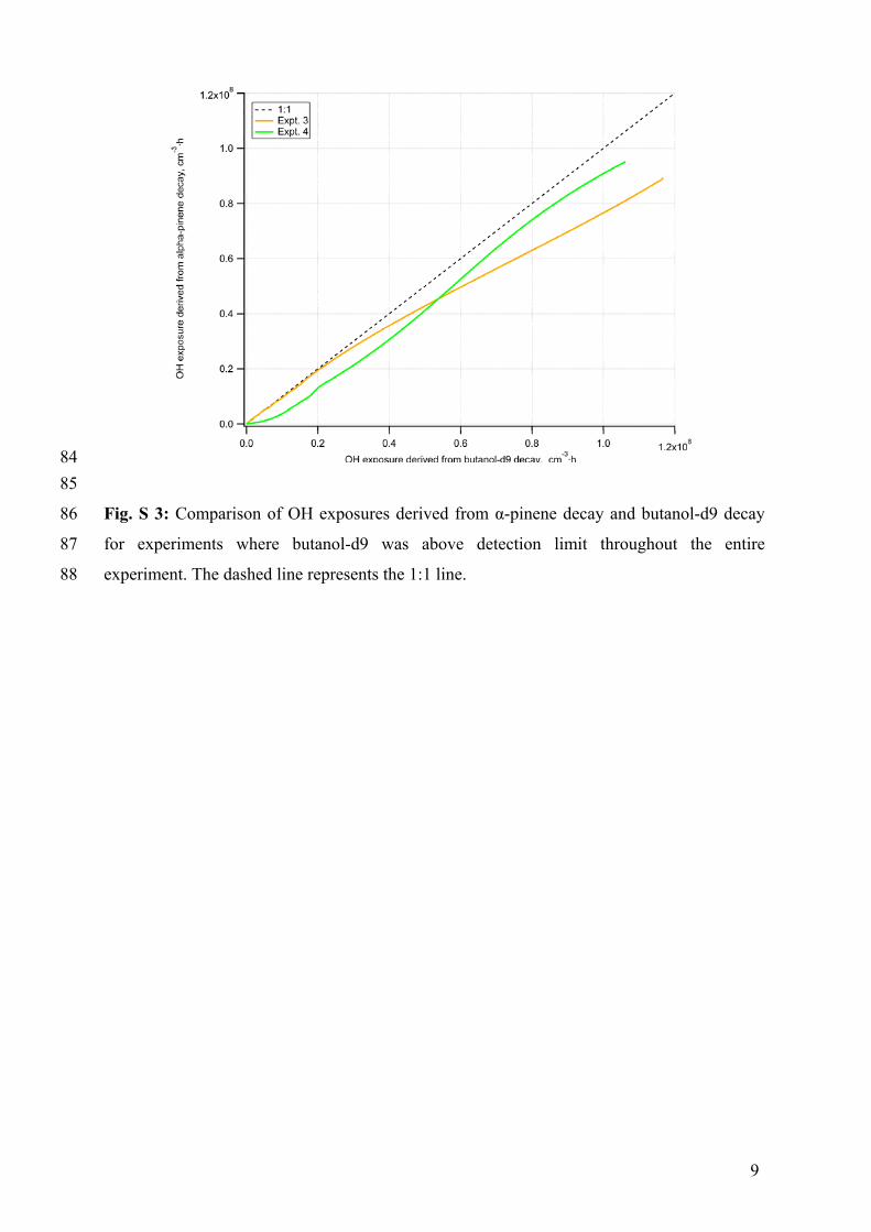
Fig. S 3: Comparison of OH exposures derived from α-pinene decay and butanol-d9 decay 86
for experiments where butanol-d9 was above detection limit throughout the entire 87
experiment. The dashed line represents the 1:1 line. 88
10
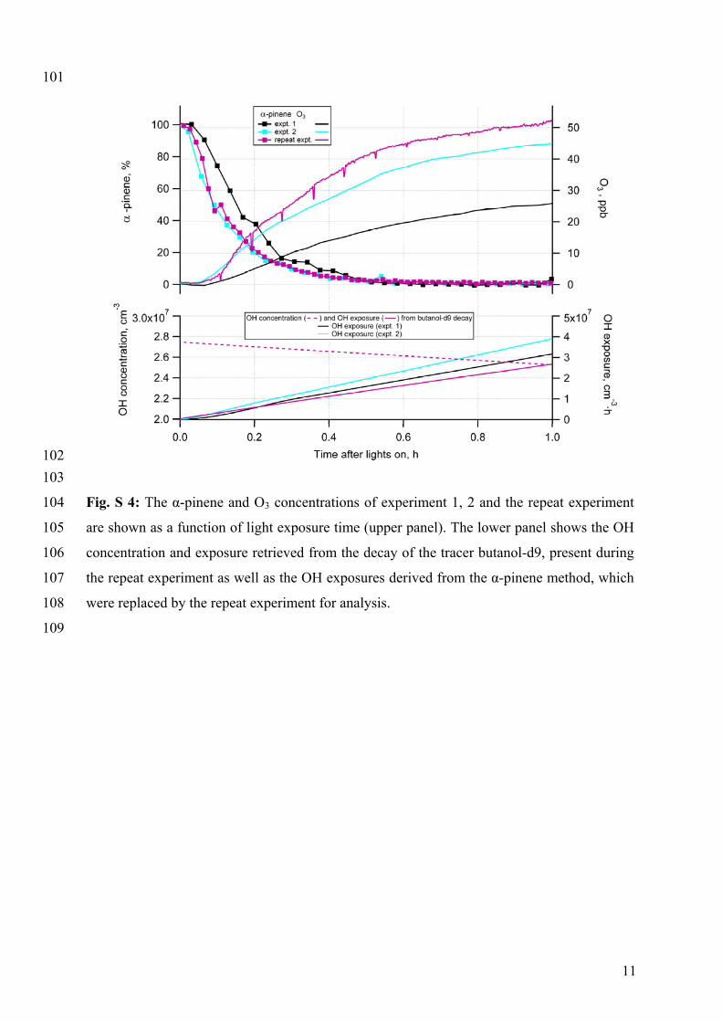
Retrieval of the OH exposure of experiment 1 and 2 from a repeat experiment 89
As the decay of α-pinene in the beginning of experiment 1 and 2 was very rapid, using the α-90
pinene method including the extrapolation to the whole experiment time leads to a possibly 91
strong overestimation of the OH exposure. For this reason a repeat experiment was conducted 92
which showed the same characteristics in α-pinene decay, but with the OH tracer butanol-d9 93
present for the whole experiment time (See Fig. S 4). The repeat experiment resembles 94
strongly experiment 2, which has the same initial α-pinene concentration (14 ppbv). During 95
experiment 1 (with an initial α-pinene concentration of 7 ppbv), the reactant decays within 96
the same time. This lower initial α-pinene concentration is also the reason for the lower O3 97
production. The replaced OH exposures derived from the α-pinene decay for experiments 1 98
(black line) and 2 (turquoise line) are shown in the lower panel together with the OH 99
exposure of the repeat experiment (purple line). 100
11
101
102
103
Fig. S 4: The α-pinene and O3 concentrations of experiment 1, 2 and the repeat experiment 104
are shown as a function of light exposure time (upper panel). The lower panel shows the OH 105
concentration and exposure retrieved from the decay of the tracer butanol-d9, present during 106
the repeat experiment as well as the OH exposures derived from the α-pinene method, which 107
were replaced by the repeat experiment for analysis. 108
109
12
110
111
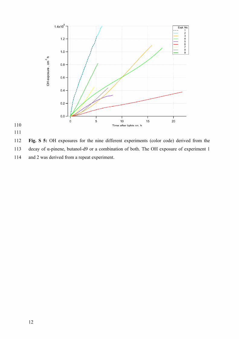
Fig. S 5: OH exposures for the nine different experiments (color code) derived from the 112
decay of α-pinene, butanol-d9 or a combination of both. The OH exposure of experiment 1 113
and 2 was derived from a repeat experiment. 114
13
115
116
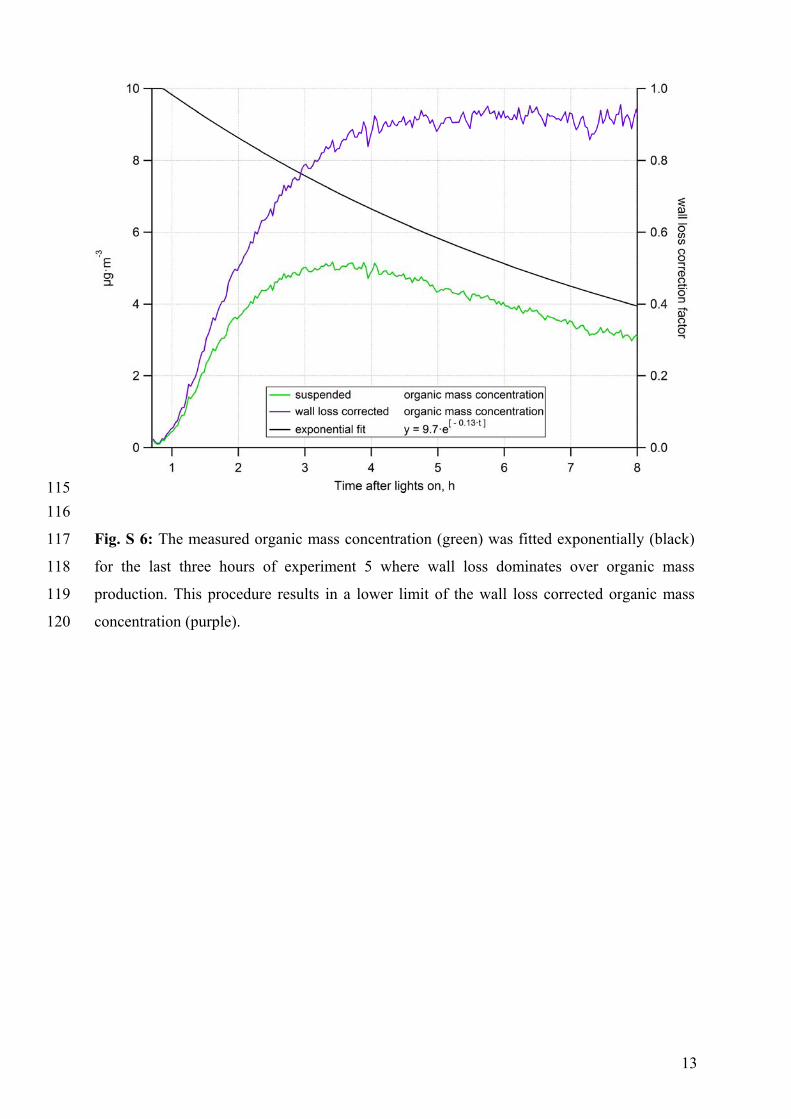
Fig. S 6: The measured organic mass concentration (green) was fitted exponentially (black) 117
for the last three hours of experiment 5 where wall loss dominates over organic mass 118
production. This procedure results in a lower limit of the wall loss corrected organic mass 119
concentration (purple). 120
14
121
122
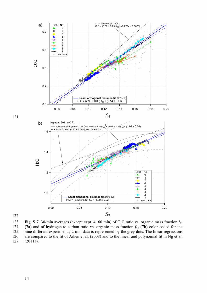
Fig. S 7. 30-min averages (except expt. 4: 60 min) of O:C ratio vs. organic mass fraction f44 123 (7a) and of hydrogen-to-carbon ratio vs. organic mass fraction f43 (7b) color coded for the 124 nine different experiments; 2-min data is represented by the grey dots. The linear regressions 125 are compared to the fit of Aiken et al. (2008) and to the linear and polynomial fit in Ng et al. 126 (2011a). 127
15
128
129
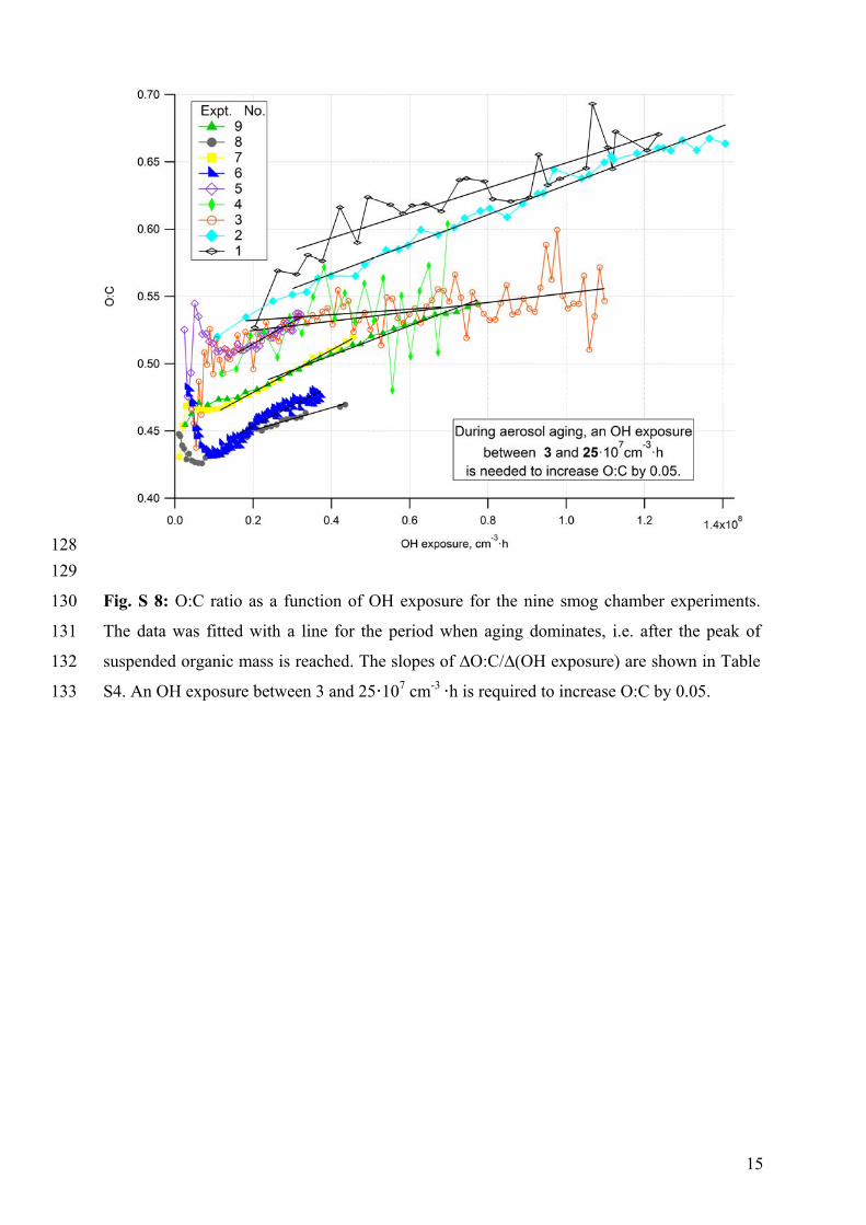
Fig. S 8: O:C ratio as a function of OH exposure for the nine smog chamber experiments. 130
The data was fitted with a line for the period when aging dominates, i.e. after the peak of 131
suspended organic mass is reached. The slopes of ∆O:C/∆(OH exposure) are shown in Table 132
S4. An OH exposure between 3 and 25·107 cm-3 ·h is required to increase O:C by 0.05. 133
16
134
135
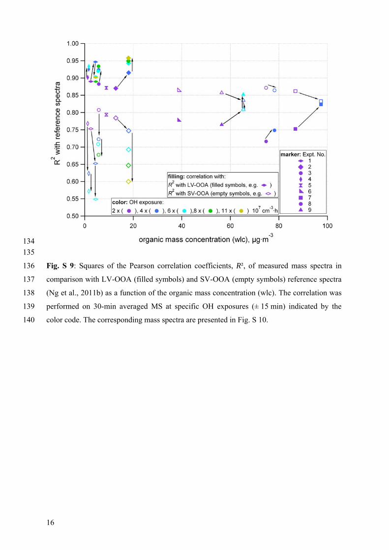
Fig. S 9: Squares of the Pearson correlation coefficients, R², of measured mass spectra in 136
comparison with LV-OOA (filled symbols) and SV-OOA (empty symbols) reference spectra 137
(Ng et al., 2011b) as a function of the organic mass concentration (wlc). The correlation was 138
performed on 30-min averaged MS at specific OH exposures (± 15 min) indicated by the 139
color code. The corresponding mass spectra are presented in Fig. S 10. 140
17
141
142
143
18
144
145
19
146
147
20
148
149
21
150
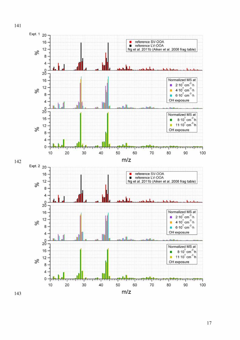
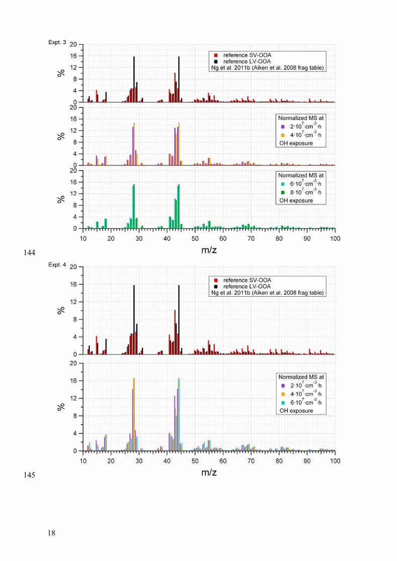
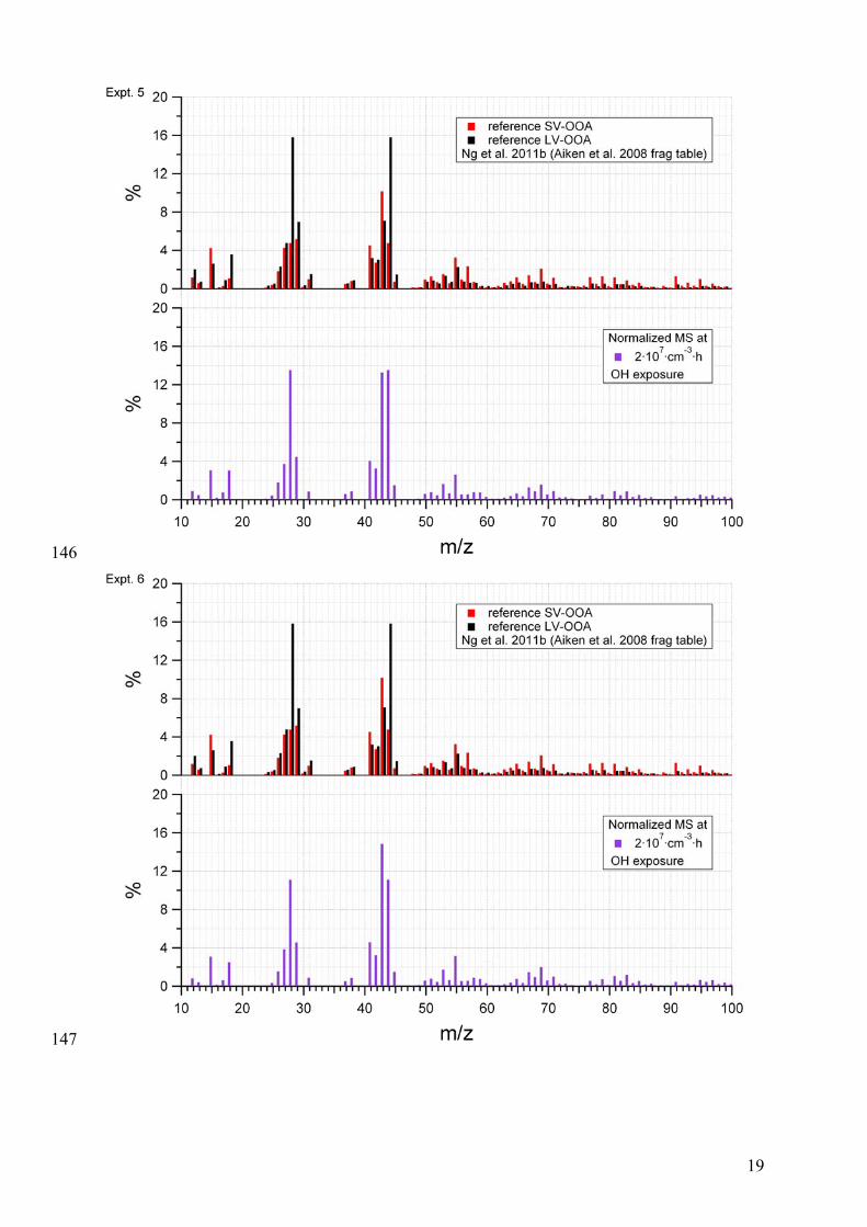
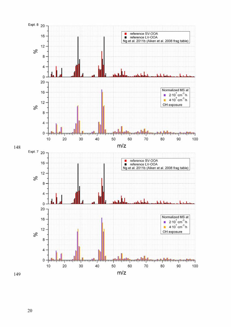
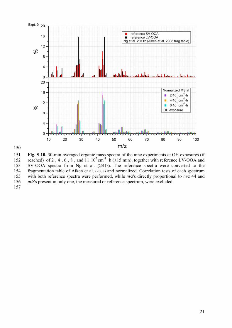
Fig. S 10. 30-min-averaged organic mass spectra of the nine experiments at OH exposures (if 151 reached) of 2·, 4·, 6·, 8·, and 11·107 cm-3 ·h (±15 min), together with reference LV-OOA and 152 SV-OOA spectra from Ng et al. (2011b). The reference spectra were converted to the 153 fragmentation table of Aiken et al. (2008) and normalized. Correlation tests of each spectrum 154 with both reference spectra were performed, while m/z's directly proportional to m/z 44 and 155 m/z's present in only one, the measured or reference spectrum, were excluded. 156 157
22
158
References 159
160
Aiken, A. C., DeCarlo, P. F., Kroll, J. H., Worsnop, D. R., Huffman, J. A., Docherty, K. S., 161 Ulbrich, I. M., Mohr, C., Kimmel, J. R., Sueper, D., Sun, Y., Zhang, Q., Trimborn, A., 162 Northway, M., Ziemann, P. J., Canagaratna, M. R., Onasch, T. B., Alfarra, M. R., 163 Prevot, A. S. H., Dommen, J., Duplissy, J., Metzger, A., Baltensperger, U., and 164 Jimenez, J. L.: O/C and OM/OC ratios of primary, secondary, and ambient organic 165 aerosols with high-resolution time-of-flight aerosol mass spectrometry, Environ. Sci. 166 Technol., 42, 4478-4485, 2008. 167
Canonaco, F., Crippa, M., Slowik, J., Baltensperger, U., and Prévôt, A. S. H.: A newly 168 developed interface for analyzing generalized Multilinear engine (ME-2) results: 169 Application on aerosol mass spectrometer data, in prep., 2013. 170
Lanz, V. A., Alfarra, M. R., Baltensperger, U., Buchmann, B., Hueglin, C., and Prevot, A. S. 171 H.: Source apportionment of submicron organic aerosols at an urban site by factor 172 analytical modelling of aerosol mass spectra, Atmos. Chem. Phys., 7, 1503-1522, 173 2007. 174
Ng, N. L., Canagaratna, M. R., Jimenez, J. L., Chhabra, P. S., Seinfeld, J. H., and Worsnop, 175 D. R.: Changes in organic aerosol composition with aging inferred from aerosol mass 176 spectra, Atmos. Chem. Phys., 11, 6465-6474, 2011a. 177
Ng, N. L., Canagaratna, M. R., Jimenez, J. L., Zhang, Q., Ulbrich, I. M., and Worsnop, D. R.: 178 Real-Time Methods for Estimating Organic Component Mass Concentrations from 179 Aerosol Mass Spectrometer Data, Environ. Sci. Technol., 45, 910-916, 2011b. 180
Paatero, P.: The multilinear engine - A table-driven, least squares program for solving 181 multilinear problems, including the n-way parallel factor analysis model, Journal of 182 Computational and Graphical Statistics, 8, 854-888, 10.2307/1390831, 1999. 183
184 185