Supplementary Material forStress Gradient Plasticity

Srinath Chakravarthy and William Curtin

July 28, 2011

In this supplementary material we provide details of the methods used or discussed in the main paper “StressGradient Plasticity” (σGP) and additional evidence for some of the conclusions in the main paper. In Section S.1we provide a few key details of the 2D discrete dislocations simulations for researchers interested in repeatingour simulations and also show examples of the actual stress-strain curves obtained both in tension and bendingand evidence of size effects in bending. In Section S.2 we provide details of the numerical procedure used in thecontinuum viscoplastic implementation of σGP. We then show that predictions of σGP are in excellent agreementwith DD results in bending.

S.1 2D Discrete dislocation simulations

S.1.1 One source surrounded by two obstaclesIn this section we show results from 2D DD simulations, of one source surrounded by two equi-spaced obstaclesin a linear stress gradient. Before we proceed, we recall that the main result of stress gradient plasticity states thatthe enhanced yield stress in the presence of a stress gradient is

τ ′Y =τY

(1− χLobs/4)(S1)

The geometry is exactly that of Figure 1 of the main paper, with the applied stress τ(x) = τapp(1 − χx). Wefirst measure on the stress on the dislocation pinned on the right obstacle as a function of the mean applied stressτapp, not allowing for any dislocations to escape from the left obstacle, which corresponds to the analytic modelabove. For various combinations of the product χLobs the analytic model is in nearly perfect agreement with thenumerical model (see Figure 1a.We then allow dislocations to escape from the left obstacle when the stress onthat obstacle reaches τobs. In this case, as the gradient product χLobs increases, there is increasing deviation fromthe analytical model, with the analytical model over predicting the flow stress. The over prediction arises becauseas dislocations escape from the high-stress side of the pile-up, additional dislocations can be nucleated from thesource, and these increase the stress acting on the low-stress side of the pile-up, and thus drive flow at smallerapplied stresses. The limiting situation, arising as χLobs approaches 4, is captured analytically by a one-sidedpile-up, i.e. a source with one obstacle on the right and no obstacle on the left (or equivalently a zero-strengthobstacle on the left), which yields

τ ′Y =1√2

τY(1− χLobs/4)

(S2)

which differs only by a factor of 1/√

(2) from Eq. S1. To capture this limit, we propose the modified form

τ ′Y =τY

(1− χLobs/4)

1

(1 + χLobs/4)1/2(S3)

1

a) b)

TTTT

TTTT T

TTTT

TTTTT

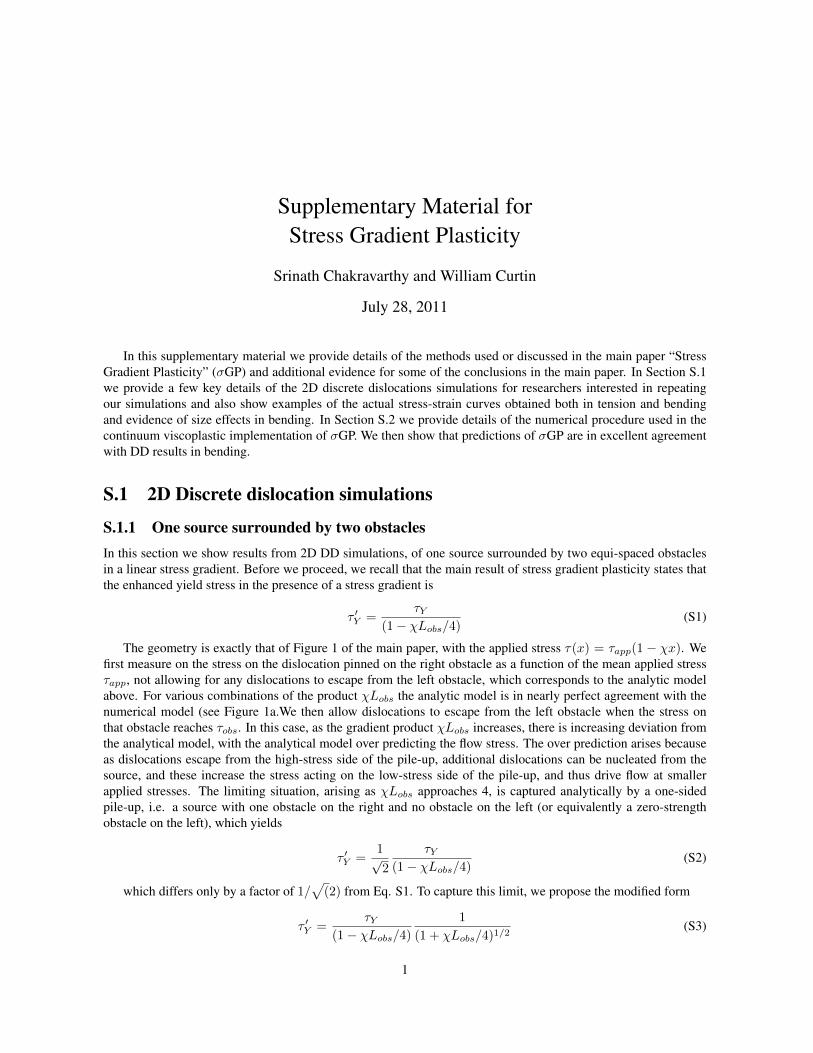
Figure S1: Comparison of DD results for a single source surrounded by two equi-spaced obstacles in a stressgradient, for all values of τY > 2τs a) No dislocation escape, eq. 1, b) With dislocation escape from left obstacle,eq. 3

Figure 1b shows that the DD results are in very good agreement with Eq. S3. Note that the predicted divergencein the flow stress as χLobs approaches 4 is also evident in the DD results. The essential features of Eq. S1 are thuspreserved.

S.1.2 2D DD of tension and bendingThe 2d DD framework is generically that of [ 1], which is well described in the literature so that only a few keydetails are provided here [ 2–4]. The test sample is a beam with width/height=3 containing slip planes on threeslip systems oriented at angles equal 30◦, 150◦ and 90◦ relative to the axis of the beam with slip plane spacingof d = 100b. Dislocation sources are distributed randomly on the slip planes with a fixed areal density ρs = 25µm−2 with randomly assigned strengths τs in the range 50 ± 10 MPa. Obstacles of strength τobs are distributedalong the slip planes with mean spacing Lobs, minimum spacing 0.5 Lobs and maximum spacing of 1.5Lobs [ 4].To avoid an artificially lower source/obstacle strength for sources near the surface that have only one (interior)obstacle, those obstacle spacings are reduced to have a maximum of 0.375Lobs, so that all source-obstacle pairsin the material have the same average flow stress. In fact, 3d DD studies show that surface-truncated sources arestronger, with the surface acting as an obstacle, which is one origin of size effects uniform loading of micropillars;we intentionally do not include this effect in our models [ 5]. By controlling combinations of τs, Lobs, and τobs,we can create materials that have the same macroscopic tensile yield stress (here 300 MPa) but differing internallength scales (Lobs), allowing us to independently probe the role of material length scales [ 4]. Beam heights rangefrom 2.0µm down to 1.0µm, with five statistical realizations of source and obstacle distributions and with averageobstacle spacings of Lobs = 0.1 − 0.6 µm for each beam size. Mechanical testing is performed by applyingboundary conditions to the ends of the beam. For tension, a uniform displacement is applied at a strain rate of103/s. For bending, a pure rotation is applied such that the strain rate at the top surface of the beam is 103/s.Because plastic flow is controlled by obstacles, the material response is very rate-insensitive so that, in spite of thehigh loading rates, the behavior is nearly identical to the quasi-static response.

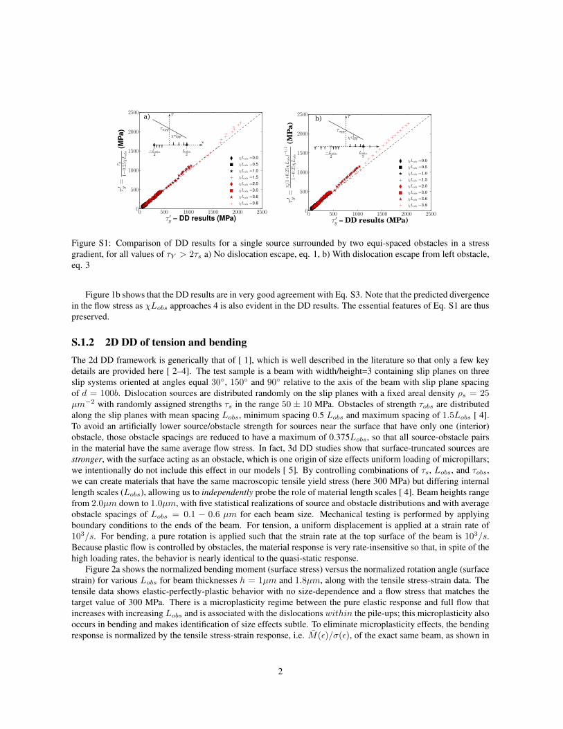
Figure 2a shows the normalized bending moment (surface stress) versus the normalized rotation angle (surfacestrain) for various Lobs for beam thicknesses h = 1µm and 1.8µm, along with the tensile stress-strain data. Thetensile data shows elastic-perfectly-plastic behavior with no size-dependence and a flow stress that matches thetarget value of 300 MPa. There is a microplasticity regime between the pure elastic response and full flow thatincreases with increasing Lobs and is associated with the dislocations within the pile-ups; this microplasticity alsooccurs in bending and makes identification of size effects subtle. To eliminate microplasticity effects, the bendingresponse is normalized by the tensile stress-strain response, i.e. M(ε)/σ(ε), of the exact same beam, as shown in

2

Figure 2b, from which clear size effects are observed.

a) b)

Figure S2: a) Stress strain response in tension (dashed lines) and bending (solid lines). b) Bending surface stressnormalized by the uniaxial tensile stress. These curves are representative of one particular statistical distributionof sources and obstacles, with material properties, E =70 GPa, ν = 0.33, b = 0.25 nm.

S.2 Continuum Viscoplastic σGP implementationSince our σGP model (Eq. 1) represents a small-scale yield stress of the material it is accommodated into acontinuum viscoplastic model simply by including the gradient term (1 − χLobs/4) in the constitutive behavior,similar to the literature for low-order εGP models [ 6, 7]. Assuming an isotropic material with elastic modulus Eand poisson’s ration ν, and small strains and rotations, the total strain rate is decomposed into the sum of the elasticand plastic strain rates as

εij = εeij + εpij (S4)

The stress can be decomposed into a volumetric part (σkk/3) and a deviatoric part sij = σij − σkk/3δij , thusgiving the volumetric and deviatoric strain rates to be

εkk = σkkν

E(S5)

and

eij =1 + ν

Esij +

3εp

2σesij (S6)

where σe =√

(3/2)sijsij is the effective stress. εp is the effective plastic strain rate and is given by

εp = ε

[σe

σ′Y f(εp)

]m(S7)

3

where ε =√

(2/3)εij εij is the effective total strain rate, and σ′Y = σY /(1−χLobs/4) as in Eq. S1, with σY thetensile yield stress, σY f(εP ) the uniaxial stress-strain curve including hardening through f(εP ) = (1+Eεp/σY )N

with strain hardening exponent N , and m the rate exponent. At the continuum level, the gradient is computed asχ =

√∇σe · ∇σe/σe. However, since a continuum model is a homogenized representation of a material with

internal length scales, it cannot be applied at scales comparable to the underlying length scale [ 8]. Rather, thegradient parameter χ(x) at point x must represent the gradient averaged over the scale of Lobs, so we use

χ(x) =1

Lobs

∫ Lobs/2

−Lobs/2

χ(x′)dx′, |x| ≥ Lobs/2 (S8)

and

χ(x) =1

Lobs

∫ Lobs/2

0

χ(x′)dx′, |x| < Lobs/2 (S9)

For pure beam bending within the (x1−x2) plane, with a beam of thickness h and the x1-axis being the neutralaxis, subject to a constant bending curvature rate κ, the non-vanishing strain rates are ε11 = −ε22 = κx2. Thetotal effective strain rate ε = 2/

√(3)κ |x2| and the effective stress is σe =

√3|σ11|. Substitution into Eq. S4 and

using the stress decomposition gives

σ11 =2E

(1 + ν)κx2

[1−

( √3 |σ11|

2σ′Y f(εp)

)m](S10)

The effective plastic strain rate is then given by

εp =2√3κx2

( √3 |σ11|

2σ′Y f(εp)

)m

(S11)

The total plastic strain rate is then calculated εp =∫ t

0εpdt. The ordinary differential equations Eqs. S10

and S11 can be solved using standard numerical algorithms [ 9], with the initial condition εp(0) = 0. Figure 3shows plots of the surface stress normalized by the tensile yield stress M/σY = 3M/2h2/σY versus the surfacestrain κh/2 for different values of Lobs/h obtained from DD simulations of beam bending, showing clearly theelevation of the initial yield stress and increase in hardening with Lobs/h and the almost perfect agreement withthe continuum σGP predictions obtained using the DD tensile data as input.

4

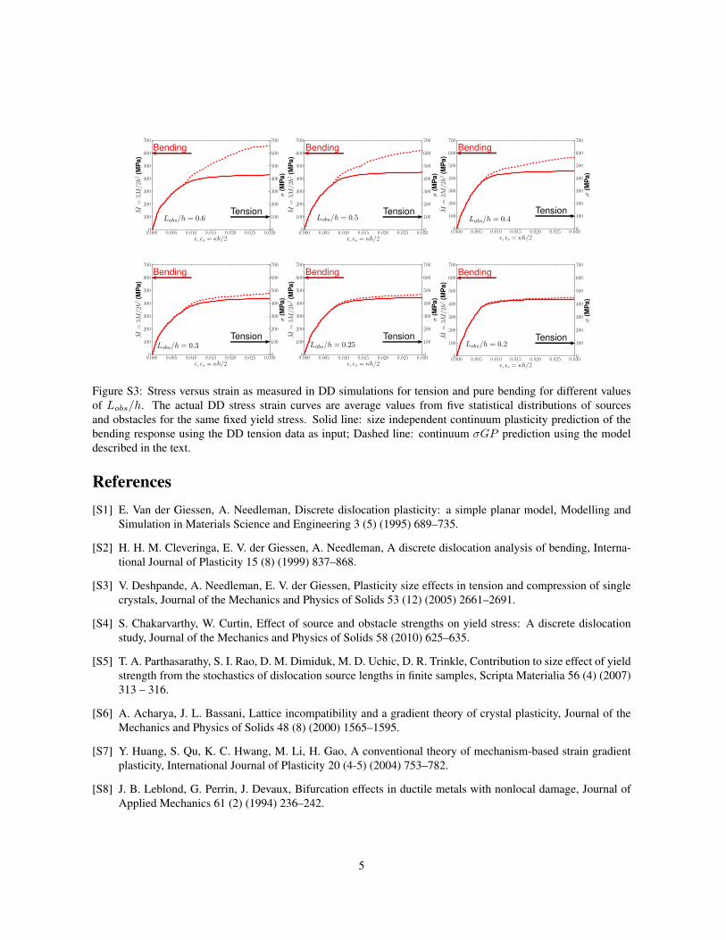
Figure S3: Stress versus strain as measured in DD simulations for tension and pure bending for different valuesof Lobs/h. The actual DD stress strain curves are average values from five statistical distributions of sourcesand obstacles for the same fixed yield stress. Solid line: size independent continuum plasticity prediction of thebending response using the DD tension data as input; Dashed line: continuum σGP prediction using the modeldescribed in the text.

References[S1] E. Van der Giessen, A. Needleman, Discrete dislocation plasticity: a simple planar model, Modelling and

Simulation in Materials Science and Engineering 3 (5) (1995) 689–735.

[S2] H. H. M. Cleveringa, E. V. der Giessen, A. Needleman, A discrete dislocation analysis of bending, Interna-tional Journal of Plasticity 15 (8) (1999) 837–868.

[S3] V. Deshpande, A. Needleman, E. V. der Giessen, Plasticity size effects in tension and compression of singlecrystals, Journal of the Mechanics and Physics of Solids 53 (12) (2005) 2661–2691.

[S4] S. Chakarvarthy, W. Curtin, Effect of source and obstacle strengths on yield stress: A discrete dislocationstudy, Journal of the Mechanics and Physics of Solids 58 (2010) 625–635.

[S5] T. A. Parthasarathy, S. I. Rao, D. M. Dimiduk, M. D. Uchic, D. R. Trinkle, Contribution to size effect of yieldstrength from the stochastics of dislocation source lengths in finite samples, Scripta Materialia 56 (4) (2007)313 – 316.

[S6] A. Acharya, J. L. Bassani, Lattice incompatibility and a gradient theory of crystal plasticity, Journal of theMechanics and Physics of Solids 48 (8) (2000) 1565–1595.

[S7] Y. Huang, S. Qu, K. C. Hwang, M. Li, H. Gao, A conventional theory of mechanism-based strain gradientplasticity, International Journal of Plasticity 20 (4-5) (2004) 753–782.

[S8] J. B. Leblond, G. Perrin, J. Devaux, Bifurcation effects in ductile metals with nonlocal damage, Journal ofApplied Mechanics 61 (2) (1994) 236–242.

5

[S9] W. H. Press, S. A. Teukolsky, W. T. Vetterling, B. P. Flannery, Numerical recipes in C (2nd ed.): the art ofscientific computing, Cambridge University Press, New York, NY, USA, 1992.URL http://portal.acm.org/citation.cfm?id=148286

6