1

Supplementary information

Supplementary Figure S1

Supplementary Figure S1- DLS results. (a) Z-average size, count rate (in kilocounts/s) and

polydispersity index (PDI = σ2/ZD

2, with σ = standard deviation and ZD = Z-average size) as

function of reaction time, insert: Number average size distribution at t = 8 and 12 minutes. (b)

Correlation data of mineralizing solution at 4, 8 and 12 min, insert shows the relative increase of

the contribution of the spheres during time as indicated by the arrows. The raw correlation data

shows the correlation time - a measure of particle size – plotted against the correlation

coefficient which is a measure of intensity but standardized at 0.7-0.9. The drops in the graphs

correspond to the presence of a particle with a certain size and can be used to describe the

presence of large particles inside the solution, as in contrast to the data on number-, volume-

and intensity-averaged size, it does not have a cut-off at 4 µm. The correlation data of the

mineralization reaction after 4 min shows us 3 distinct drops at around 200 nm, 40 µm and even

larger species. The smallest size corresponds to the collapsed polymer aggregates, the larger

sizes correspond to the low-density polymeric superstructures observed in cryo-TEM.

2

Supplementary Figure S2

Supplementary Figure S2 - Close-up of pH/Ca2+

-concentration upon stepwise adding the

phosphate stock to the calcium-stock. During this particular reaction the electrode was

immersed into the calcium stock before the addition of the phosphate stock. The addition of the

phosphate stock leads to a drop in the calcium concentration in the reaction solution, while the

pH stays constant. The calcium electrode responds immediately and is also immediately stable.

After the addition no changes in the calcium concentration or pH are observed with in the first

10 minutes, during the development of the branched polymeric assemblies.

3

Supplementary Figure S3

Supplementary Figure S3 - Representation of the mineralization experiment, showing the

different stages with corresponding time points, chemical formulas or names and the amounts

of Ca bound (∆Ca1-4), phosphate bound (∆P1-4) and H+-released (∆H1-4) in between the different

stages.

4

Supplementary Figure S4

y = 9,993E-05x + 2,520E-07

R2 = 1,000E+00

y = 6,829E-05x + 9,885E-06

R2 = 9,998E-01

y = 3,164E-05x - 9,633E-06

R2 = 9,991E-01

0

0,0005

0,001

0,0015

0,002

0,0025

0,003

0 2 4 6 8 10 12 14 16 18 20

time (min)

calc

ium

/ a

dd

ed

NaO

H(m

mo

l)

total calcium

bound calcium

free calcium

added NaOH

Linear (total

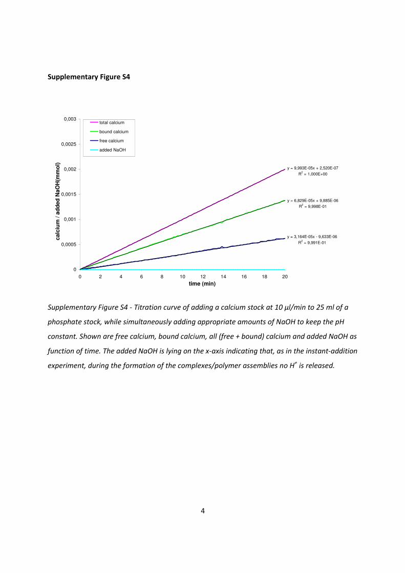
Supplementary Figure S4 - Titration curve of adding a calcium stock at 10 µl/min to 25 ml of a

phosphate stock, while simultaneously adding appropriate amounts of NaOH to keep the pH

constant. Shown are free calcium, bound calcium, all (free + bound) calcium and added NaOH as

function of time. The added NaOH is lying on the x-axis indicating that, as in the instant-addition

experiment, during the formation of the complexes/polymer assemblies no H+ is released.

5

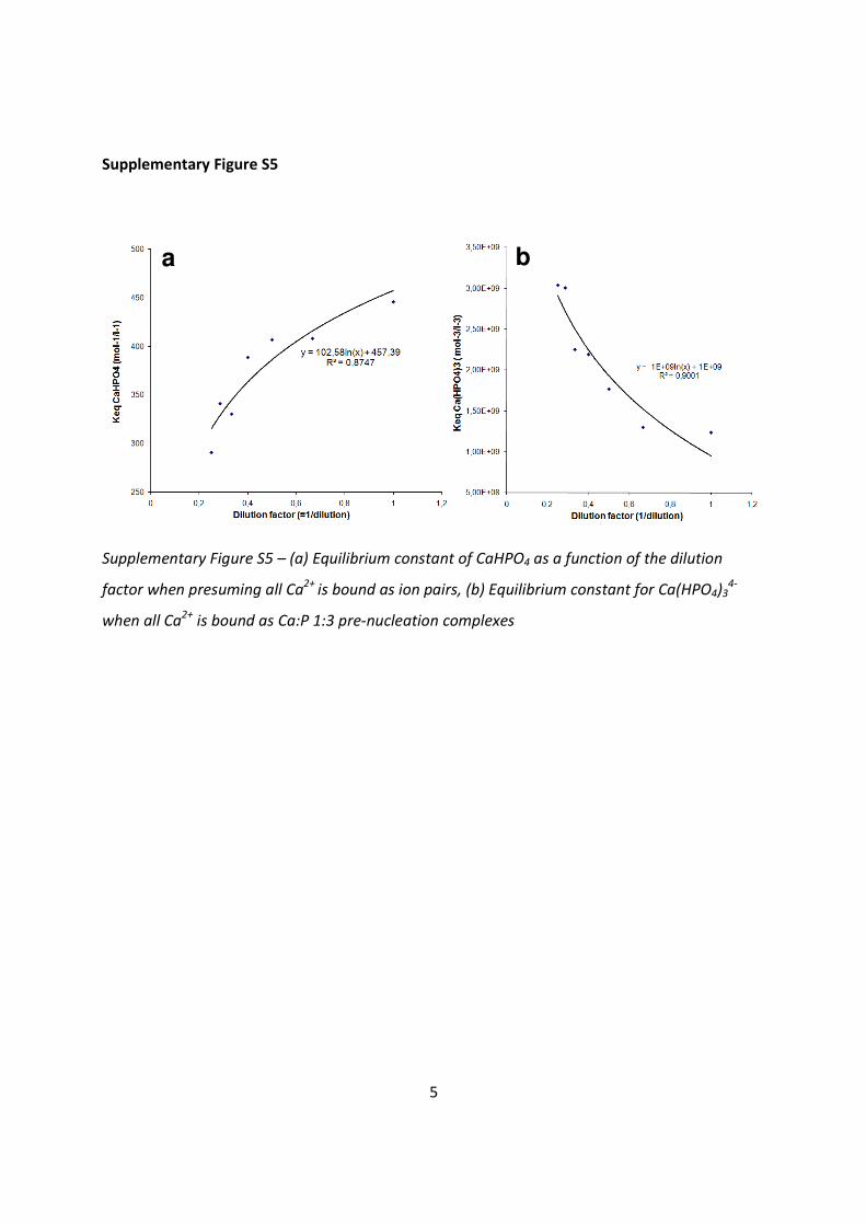
Supplementary Figure S5

Supplementary Figure S5 – (a) Equilibrium constant of CaHPO4 as a function of the dilution

factor when presuming all Ca2+

is bound as ion pairs, (b) Equilibrium constant for Ca(HPO4)34-

when all Ca2+

is bound as Ca:P 1:3 pre-nucleation complexes

a b

6

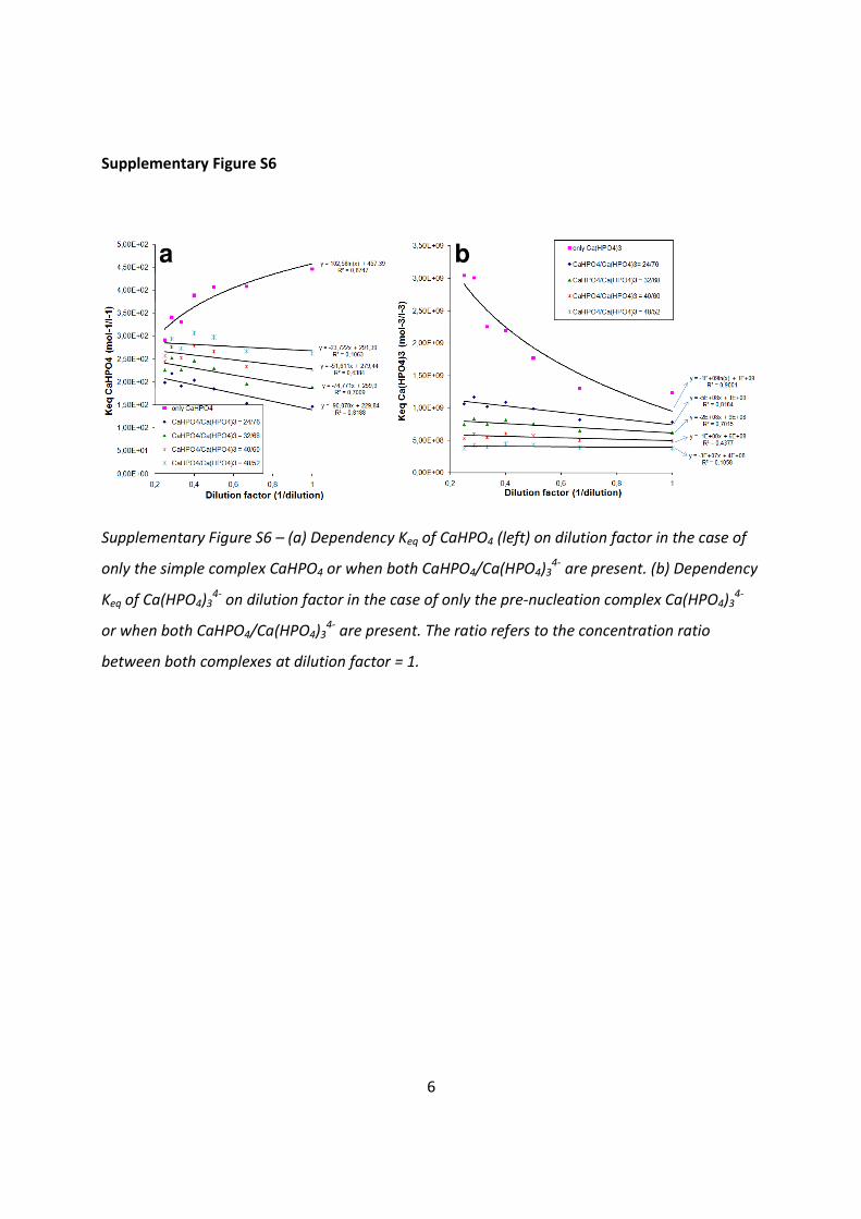
Supplementary Figure S6

Supplementary Figure S6 – (a) Dependency Keq of CaHPO4 (left) on dilution factor in the case of

only the simple complex CaHPO4 or when both CaHPO4/Ca(HPO4)34-

are present. (b) Dependency

Keq of Ca(HPO4)34-

on dilution factor in the case of only the pre-nucleation complex Ca(HPO4)34-

or when both CaHPO4/Ca(HPO4)34-

are present. The ratio refers to the concentration ratio

between both complexes at dilution factor = 1.

b a

7

Supplementary Figure S7

Supplementary Figure S7 - Structure pre-nucleation complex as derived from ab-initio

calculations, projected from top view (a) or side view (b). a* and b* show the conformation of

the hydration waters surrounding the complex. The planar arrangement of the phosphates can

be explained by the significant repulsion between individual phosphates. As represented in

figure a* and b*, water binds preferably by H-bonds to the oxygens of the phosphate, whereas

the sides of the calcium are rather bare only binding to 1 H2O molecule. The size of the complex

and the corresponding atomic distances derived from the ab-initio calculations correspond well

to values calculated for the complex structure according to various effective ionic radii from

literature74

(See also supplementary Table S3). The coordination number of Ca2+

was found to be

7, which is within the range of reported coordination numbers74

for Ca2+

(6-12).

= Ca2+

= P5+

= O2-

= H+

a b

a* b*

double bond

single bond

H-bond

8

Supplementary Figure S8A

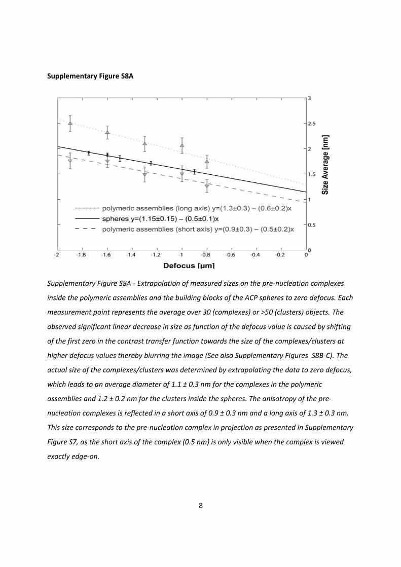
Supplementary Figure S8A - Extrapolation of measured sizes on the pre-nucleation complexes

inside the polymeric assemblies and the building blocks of the ACP spheres to zero defocus. Each

measurement point represents the average over 30 (complexes) or >50 (clusters) objects. The

observed significant linear decrease in size as function of the defocus value is caused by shifting

of the first zero in the contrast transfer function towards the size of the complexes/clusters at

higher defocus values thereby blurring the image (See also Supplementary Figures S8B-C). The

actual size of the complexes/clusters was determined by extrapolating the data to zero defocus,

which leads to an average diameter of 1.1 ± 0.3 nm for the complexes in the polymeric

assemblies and 1.2 ± 0.2 nm for the clusters inside the spheres. The anisotropy of the pre-

nucleation complexes is reflected in a short axis of 0.9 ± 0.3 nm and a long axis of 1.3 ± 0.3 nm.

This size corresponds to the pre-nucleation complex in projection as presented in Supplementary

Figure S7, as the short axis of the complex (0.5 nm) is only visible when the complex is viewed

exactly edge-on.

9

Supplementary Figure S8B

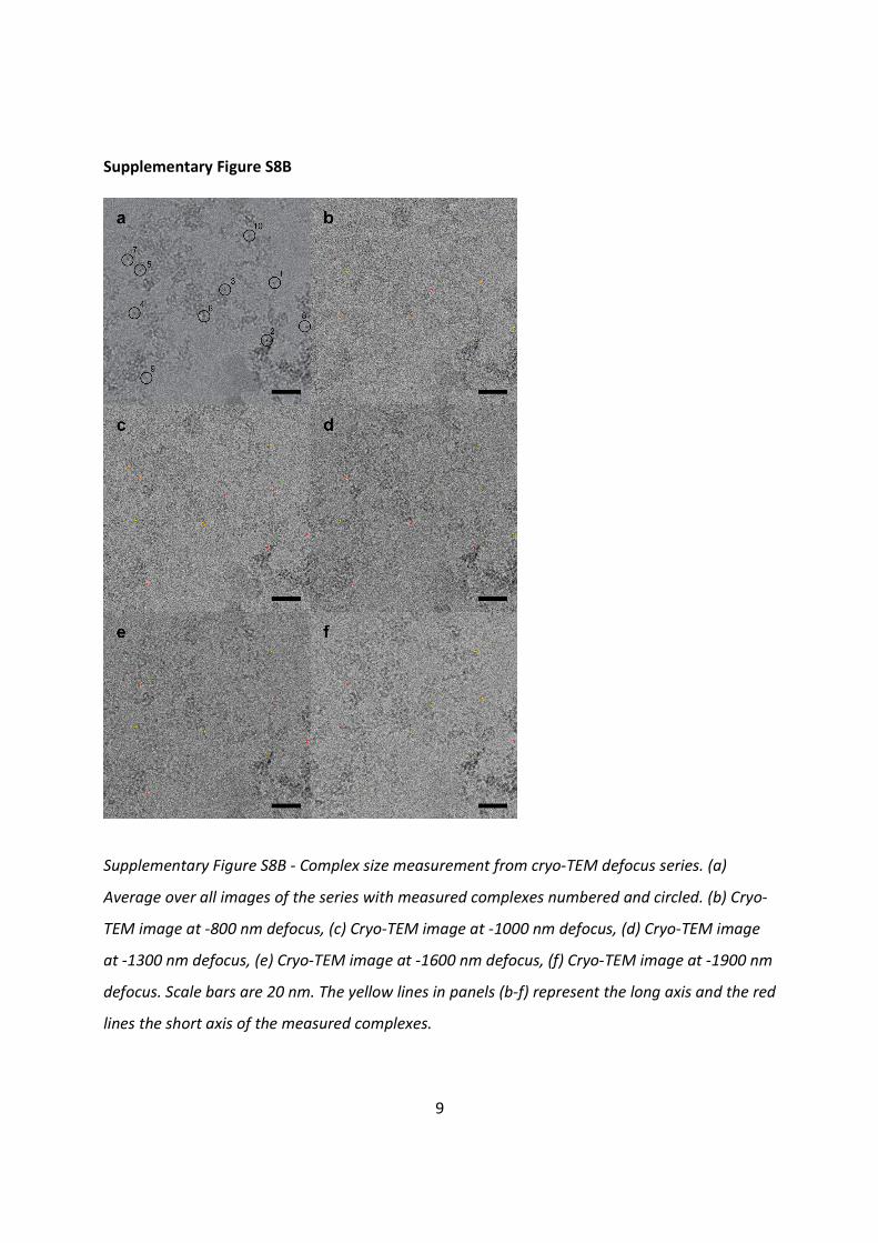
Supplementary Figure S8B - Complex size measurement from cryo-TEM defocus series. (a)

Average over all images of the series with measured complexes numbered and circled. (b) Cryo-

TEM image at -800 nm defocus, (c) Cryo-TEM image at -1000 nm defocus, (d) Cryo-TEM image

at -1300 nm defocus, (e) Cryo-TEM image at -1600 nm defocus, (f) Cryo-TEM image at -1900 nm

defocus. Scale bars are 20 nm. The yellow lines in panels (b-f) represent the long axis and the red

lines the short axis of the measured complexes.

10

Supplementary Figure S8C

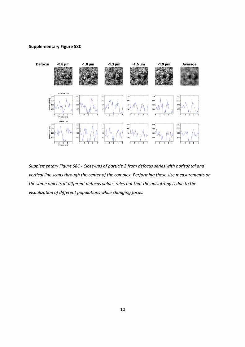
Supplementary Figure S8C - Close-ups of particle 2 from defocus series with horizontal and

vertical line scans through the center of the complex. Performing these size measurements on

the same objects at different defocus values rules out that the anisotropy is due to the

visualization of different populations while changing focus.

11

Supplementary Figure S8D

Supplementary Figure S8D - Cryo-TEM images of mineralization product and initial buffers

acquired at -1000 nm defocus. A) CaP polymer, b) Tris buffer and 10 mM CaCl2, c) Tris buffer and

10 mM K2HPO4. Both Tris buffered-saline controls do not show any signs of polymeric

assemblies. Scale bars are 50 nm.

12

Supplementary Figure S9

Supplementary Figure S9 - Fractal dimension analysis on Cryo-Tomograms. (a-d) cross-sections

of tomograms of branched polymeric assemblies and spheres, before (a+c) and after (b+d)

segmentation. (e+f) 3D surface rendering of segmented tomograms of polymer assemblies and

spheres, respectively. (g) box size vs. box number plot with corresponding fractal dimensions.

The fractal dimension was determined from a linear fit in the log-log plot using box sizes

between 4 and 128 pixel edge length to avoid artifacts due to noise and defocus effects,

respectively.

13

Supplementary Figure S10

Supplementary Figure S10 - FTIR spectra on samples from AFM experiments quenched at times

shown in figure. Solution supersaturations were σHAP = 3.36, σOCP = 1.76 and σACP = 0.04. Peaks

at 560, 599, 877 and 1036 are characteristic of OCP. FTIR was performed on samples preserved

as described in the Methods section.

14

Supplementary Figure S11

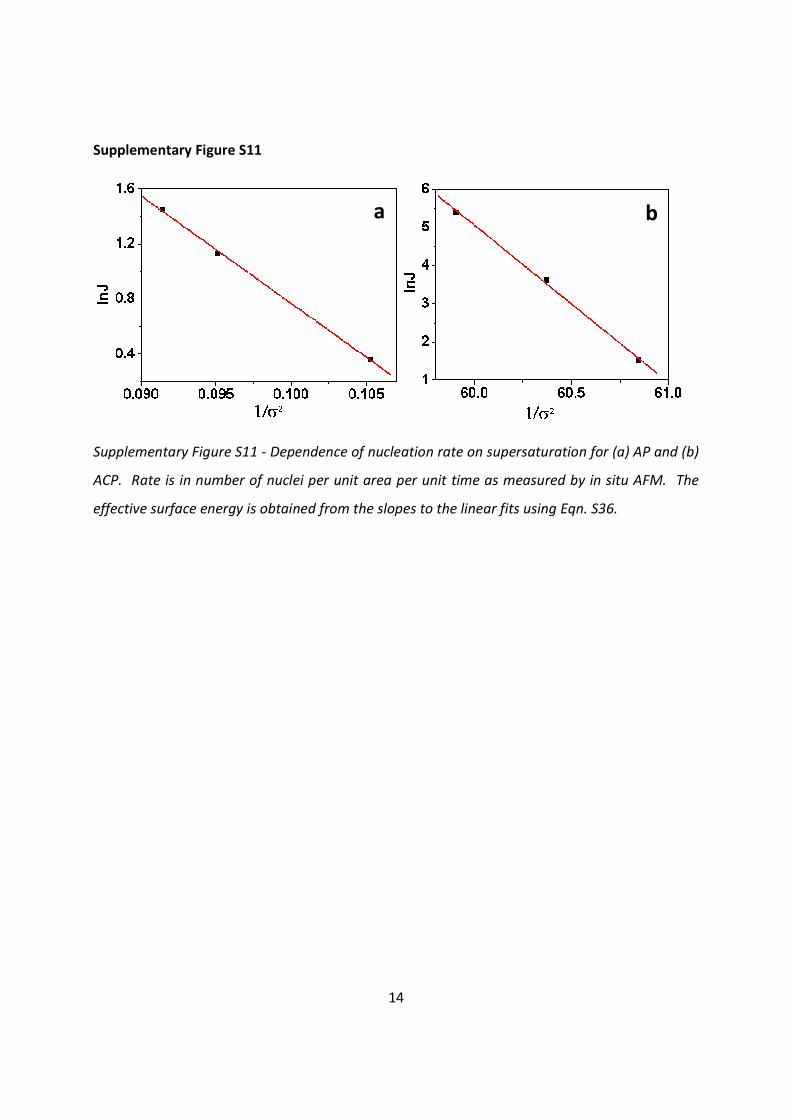
Supplementary Figure S11 - Dependence of nucleation rate on supersaturation for (a) AP and (b)

ACP. Rate is in number of nuclei per unit area per unit time as measured by in situ AFM. The

effective surface energy is obtained from the slopes to the linear fits using Eqn. S36.

a b

15

Supplementary Figure S12

Supplementary Figure S12 - SEM-images of filtrated + dried calcium phosphate samples at t = 18

min, 51 min, 106 min and 183 min showing typical morphologies expected for ACP and

OCP/HAP.

16

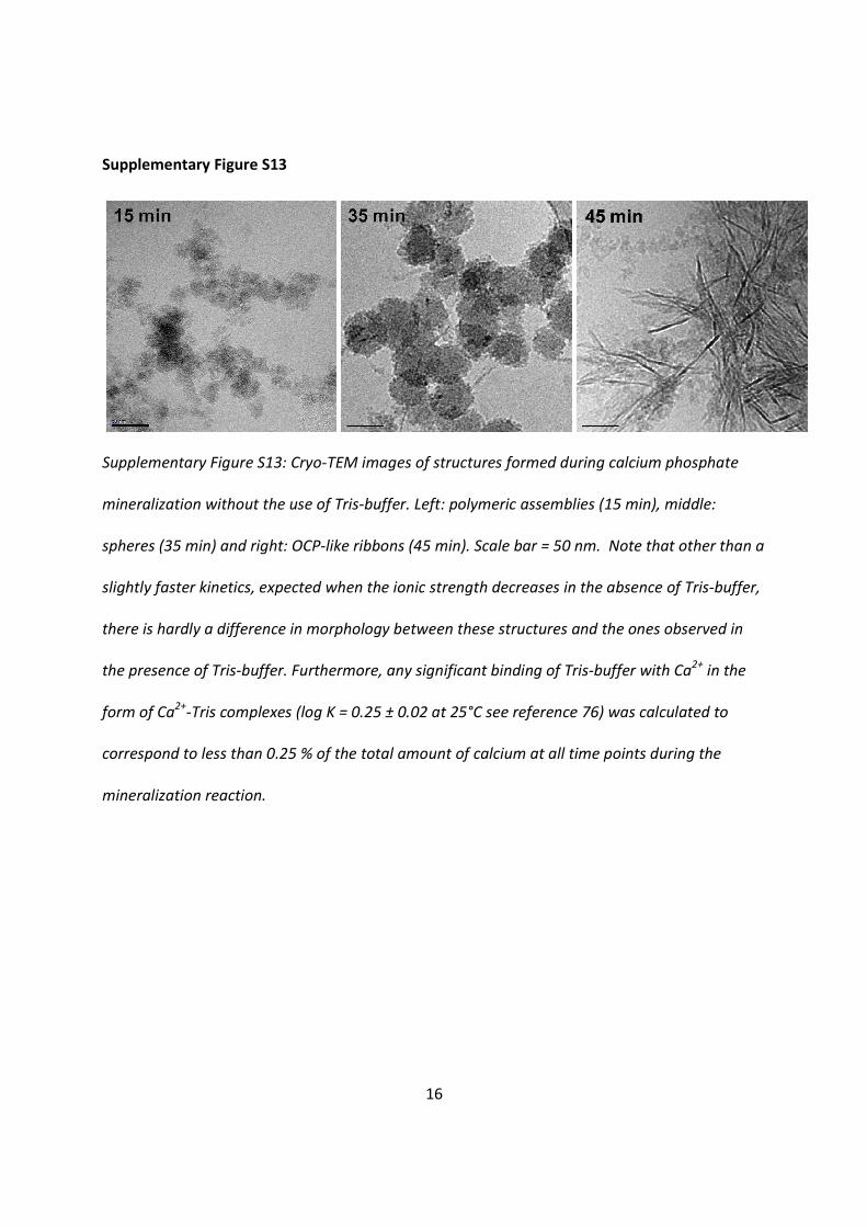
Supplementary Figure S13

Supplementary Figure S13: Cryo-TEM images of structures formed during calcium phosphate

mineralization without the use of Tris-buffer. Left: polymeric assemblies (15 min), middle:

spheres (35 min) and right: OCP-like ribbons (45 min). Scale bar = 50 nm. Note that other than a

slightly faster kinetics, expected when the ionic strength decreases in the absence of Tris-buffer,

there is hardly a difference in morphology between these structures and the ones observed in

the presence of Tris-buffer. Furthermore, any significant binding of Tris-buffer with Ca2+

in the

form of Ca2+

-Tris complexes (log K = 0.25 ± 0.02 at 25°C see reference 76) was calculated to

correspond to less than 0.25 % of the total amount of calcium at all time points during the

mineralization reaction.

17

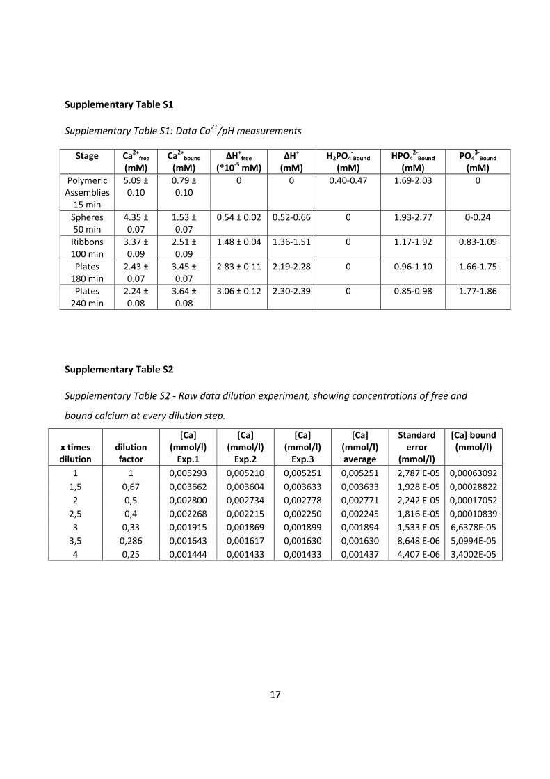
Supplementary Table S1

Supplementary Table S1: Data Ca2+

/pH measurements

Stage Ca2+

free

(mM)

Ca2+

bound

(mM)

ΔH+

free

(*10-5

mM)

ΔH+

(mM)

H2PO4-Bound

(mM)

HPO42-

Bound

(mM)

PO43-

Bound

(mM)

Polymeric Assemblies

15 min

5.09 ± 0.10

0.79 ± 0.10

0 0 0.40-0.47 1.69-2.03 0

Spheres 50 min

4.35 ± 0.07

1.53 ± 0.07

0.54 ± 0.02 0.52-0.66 0 1.93-2.77 0-0.24

Ribbons 100 min

3.37 ± 0.09

2.51 ± 0.09

1.48 ± 0.04 1.36-1.51 0 1.17-1.92 0.83-1.09

Plates 180 min

2.43 ± 0.07

3.45 ± 0.07

2.83 ± 0.11 2.19-2.28 0 0.96-1.10 1.66-1.75

Plates 240 min

2.24 ± 0.08

3.64 ± 0.08

3.06 ± 0.12 2.30-2.39 0 0.85-0.98 1.77-1.86

Supplementary Table S2

Supplementary Table S2 - Raw data dilution experiment, showing concentrations of free and

bound calcium at every dilution step.

x times

dilution

dilution

factor

[Ca]

(mmol/l)

Exp.1

[Ca]

(mmol/l)

Exp.2

[Ca]

(mmol/l)

Exp.3

[Ca]

(mmol/l)

average

Standard

error

(mmol/l)

[Ca] bound

(mmol/l)

1 1 0,005293 0,005210 0,005251 0,005251 2,787 E-05 0,00063092

1,5 0,67 0,003662 0,003604 0,003633 0,003633 1,928 E-05 0,00028822

2 0,5 0,002800 0,002734 0,002778 0,002771 2,242 E-05 0,00017052

2,5 0,4 0,002268 0,002215 0,002250 0,002245 1,816 E-05 0,00010839

3 0,33 0,001915 0,001869 0,001899 0,001894 1,533 E-05 6,6378E-05

3,5 0,286 0,001643 0,001617 0,001630 0,001630 8,648 E-06 5,0994E-05

4 0,25 0,001444 0,001433 0,001433 0,001437 4,407 E-06 3,4002E-05

18

Supplementary Table S3

Supplementary Table S3 - Size of pre- nucleation complexes and corresponding atomic distances

according to ab-initio calculations (bold) and from calculations on the structure using reported

ionic radii from literature74

. Radial distribution function data on ACC by Posner41

are given in

brackets.

Atomic distances (Å) Structure Size (Å)

Ca-O Ca-P P-O O-O P-P

11.0 (l)

12.0-13.4 (l) Pre-nucleation

complex 5.0 (h)

5.6 (h)

2.47 ± 0.06

2.4 (2.3)

3.03 ± 0.03

3.2-3.9 (3-6)

1.55 ± 0.02

1.5 (1.5)

2.45 ± 0.01

2.5 (2.3)

5.1 ± 0.3

5.6-6.8 (3-6)

11.0 (l)

11.9-12.6 (l) Pre-nucleation

complex-H+

5.0 (h)

5.6 (h)

2.47 ± 0.06

2.4 (2.3)

3.03 ± 0.03

3.2-3.9 (3-6)

1.59 ± 0.01

1.5 (1.5)

2.45 ± 0.01

2.5 (2.3)

5.1 ± 0.3

5.5-6.8 (3-6)

Supplementary Table S4

Supplementary Table S4 - Ca/P ratio measured by EDX of filtrated + dried sample at different

stages (n = 10)

Sample Ca/P ratio (± error)

18 min 1.48 ± 0.06 51 min 1.45 ± 0.02 106 min 1.45 ± 0.03 183 min 1.51 ± 0.09 239 min 1.46 ± 0.02

19

SUPPLEMENTARY METHODS

DLS investigation + zeta potential measurements

Dynamic light scattering (DLS) and zeta potential measurements were performed on a Malvern

Zetasizer Nano ZS Series (Malvern Instruments Limited, UK) with a 633 nm, 4mW HeNe laser,

measurement angle 173°; 20 °C). Measurements were averaged over 11 runs of 10 s. The

refractive index of apatite (n = 1.63) and viscosity and refractive index of phosphate buffer

saline (PBS, η = 1.0041 (20 °C), n = 1.33) were used for the calculations. Zeta potentials were

measured in transmission at a 50V effective voltage (average over 100 runs). The Von

Smoluchowski equation55 was applied, considering the high ionic strength used (I = 0.2 M) and

size of the polymeric aggregates (> 100 nm).

Calculation chemistry of calcium phosphate

Control over physiochemical conditions/ process parameters

Ca2+-ISE

To enable a quantitative interpretation of the Ca2+-ISE measurements, the physicochemical

conditions during the experiment regarding pH, temperature and ionic strength (pH = 7.4-7.2, t

= 20 °C, I = 0.2-0.22) were kept as close as possible to the Ca2+ - calibration (pH = 7.4, t = 20 °C, I

= 0.2, R2 calibration curve = 1). Furthermore, as the Ca2+-ISE is pH-dependent and formed

calcium phosphate could interfere with the Ca2+-ISE increasingly during time, the Ca2+-ISE

measurement was stopped after 4h, where both pH and Ca2+ measurements reach a stable

plateau (pH = 7.167, Ca2+ concentration = 2.24 ± 0.22 mmol/l). An additional experiment was

20

performed where it was observed that in the used pH-range, the Ca2+-electrode is independent

of the pH.

As a further control, the Ca2+-concentration at t = 4h was validated using ICP-OES

measurements of the supernatant (Ca2+-concentration = 2.38 ± 0.05 mmol/l). As at this time

point concentrations of ions/complexes are dictated by the precipitated OCP-phase, the Ksp of

the OCP-phase does not allow high concentrations of these complexes as was also calculated

using equilibrium constants derived from the dilution experiment described later in the

Supplementary Methods section (max. 4% of complexes). The ICP measurement of the solution

therefore should correspond to the Ca2+-ISE measurements. Although differences in ionic

strength between the calibration experiment and the actual precipitation reaction are small, to

correct the Ca2+-activity for this small difference, the ionic strength (I) of the solution at any

time point was calculated according to the following equation where ci = concentration of

species i with charge zi.

2

12

1i

n

i

i zcI ⋅⋅= ∑=

[S1]

Accordingly, while the total ionic strength (I = 0.2-0.22) surpasses the limit for extended Debye-

Hückel61, activity coefficients (γ) were calculated according to a modified version of the Davies

Extended Debye-Hückel Equation at 20°C48,62 that has reported to work well for aqueous

solutions in the range of 10-3 to 1 M62 .

21

( )

⋅−

+⋅⋅=− Ib

IBa

Izii

15046.0log

2γ [S2]

with Ba = 1.0 and b = 0.2

As especially the value for the linear coefficient (b) is reported to be dependent on, for

example, the type of electrolyte used62, activity coefficients were calculated upon varying b

from 0.1 to 0.3, showing no significant differences in species concentration. Similarly, the value

for Ba was varied from 1.0 to 1.5 resulting only in minor changes in species concentration.

Furthermore, as this equation is only valid for free ions in solution, the ionic strength of the

solution (I) was corrected for the formation of ion complexes/precipitates by subtracting the

complexed/precipitated ions from the original concentration. Due to the high concentration of

especially NaCl and Trizma-buffer in solution, contribution of ion complexes to the total ionic

strength of the solution was calculated to be negligibly small (max. 0.0064 M on a total of 0.22

M).

pH-electrode

As the pH-electrode used is accurate to +/- 0.001 pH unit, this ensures us of enough sensitivity

to visualize even small changes in phosphate chemistry. For example, the pH drop from

polymeric assemblies to spheres (7.425 � 7.367) corresponds to the release of 0.55 – 0.65 mM

H+, which is 58x the accuracy limit.

22

Control over thermodynamic pathway

As the pH does not drop below 7.0, the thermodynamically stable end product of the

mineralization reaction is apatite17. This structure was also confirmed by Cryo-TEM, electron

diffraction and in-situ FTIR on samples > 3days of incubation. The calcium phosphate phase

after 4h of reaction is OCP, as confirmed by in-situ SAXS and electron diffraction, in situ FTIR

and ICP-OES (Ca/P = 1.33 ± 0.02). OCP is described as an intermediate for apatite formation in

solution23-24.

Control over phosphate species in solution

During the whole mineralization reaction, from the observed pH-range (pH = 7.2-7.4) we can

calculate that > 99.9% of the phosphate in solution (H2PO4-, HPO4

2-, PO43-) is described by the

following equilibrium:

H2PO4- HPO4

2- + H+ (pKa = 7.21). [S3]

Chemical reactions

During the mineralization experiment a pH decrease was observed. Based on the phosphate

equilibrium, this pH-decrease can be caused by different types of reactions in which calcium

phosphate is involved. As the model can only calculate the average calcium phosphate

chemistry, the end-products of the reactions as described in this section do not have to be one

specific calcium phosphate but can represent a mixture of multiple calcium phosphate species.

23

Formation of a calcium phosphate species at time t=0

During the formation of a calcium phosphate species, the pH will decrease when Ca2+

effectively binds with PO43-,HPO4

2- or with H2PO4- and HPO4

2- in a ratio lower than the ratio

between both species present in solution (see Equation [S3]). Conversely, a pH increase will be

observed when calcium binds phosphate in a higher H2PO4-/HPO4

2- ratio or solely with H2PO4-.

As upon the formation of complexes or polymeric assemblies at t = 0 the Ca2+ is bound without

any observable pH-decrease (Supplementary Figure S2), this phenomenon can only be

described by a reaction of Ca2+ with H2PO4-/HPO4

2- where the ratio between H2PO4- and HPO4

2-

corresponds to the exact ratio of both species in solution (Equation [S4]). At the average pH =

7.425, this ratio is H2PO4-/HPO4

2- = 0.190/0.810, leading to the overall chemistry of

Ca((H2PO4)0.19(HPO4)0.81)x2-1.81*x

, according to the following reaction scheme:

Overall reaction

Ca2+ + x*0.19*H2PO4- + x*0.81*HPO4

2- � Ca((H2PO4)0.19(HPO4)0.81)x 2-1.81*x

[S4]

We want to note that:

1. Theoretically, Ca2+ can also bind to a certain mixture of H2PO4-/HPO4

2-/PO43- in such a

way that the pH stays constant as well. However, from in-situ IR the first signal that

exclusively can be attributed to PO43- (1021 cm-1) arises when the ribbon-like aggregates

appear. The pattern of the calcium phosphate species at t=0 can be attributed to the

overlap / broadening of the signals of free HPO42-/H2PO4

- in solution. Furthermore, to

keep the pH stable at the used pH, the formation of a significant amount of Cax(PO4)y

24

species implies the formation of even more species containing H2PO4-. As we have a

solution with mostly HPO42- ions, the presence of significant amounts of both Cax(PO4)y

and Cax(H2PO4)y species is very unlikely due to the large difference in the pKa of the

bound phosphates. This behavior was observed for the known CaP-ion pairs (CaPO4-,

CaHPO4 and CaH2PO4+), where the predicted pH-dependency of these ion pairs63 shows

only limited overlap between CaPO4- and CaH2PO4

+.

2. The overall reaction as described above can be divided into the concomitant formation

of multiple calcium phosphate species like the earlier described calcium phosphate ion

pairs 63,64.

3. In the case of the formation of an equilibrium species, the one-way arrow as described

above can also be read as a two-way arrow.

Reaction of calcium phosphate species with Ca2+ from the solution

After the formation of the pre-nucleation species, a simultaneous decrease of pH and Ca2+ was

observed upon the formation of the spheres, ribbons and finally OCP plates. Such a behavior

can be explained by a reaction in which bound phosphate releases protons upon the attraction

of Ca2+ from the solution (Equations [S5-S6]).

Cax(H2PO4)y(HPO4)z2x-y-2z + a Ca2+ � Cax+a (H2PO4)y-b (HPO4)z+b

2x-(y-b)-2(z+b) + b H+ [S5]

Cax(HPO4)y(PO4)z2x-2y-3z + a Ca2+

� Cax+a(HPO4)y-b(PO4)z+b2x -2(y-b)-3(z+b) + b H+ [S6]

25

Reaction of calcium phosphate species with calcium and phosphate from solution

In addition to reactions [S5] and [S6], calcium phosphate species can also attract new

phosphate from the solution at every phase transition. Taking into account the overall pH

decrease, such an event effectively will remove HPO42- from the equilibrium (Equation [S3]) and

release of H+. The amount of H+ released here is equal to the fraction of H2PO4- in solution and

therefore depends on the pH. Furthermore, as binding of PO43- is equivalent to binding HPO4

2-

and concomitant proton release from the bound HPO42- (Equation [S6]), for the average

chemistry only reactions [S7-S8] are of importance.

Cax(H2PO4)y(HPO4)z2x-y-2z + a HPO4

2- + b Ca2+ � Cax+b(H2PO4)y(HPO4)z+a2(x+b)-y-2(z+a) [S7]

Cax(HPO4)y(PO4)z2x-2y-3z + a HPO4

2- + b Ca2+ � Cax+b(HPO4)y+a(PO4)z2(x+b)-2(y+a)-3z [S8]

Side reactions

Upon designing the experiment, the possible incorporation of CO2 into the system is taken into

account. The used reaction solutions as well as both stocks are equilibrated with the CO2 from

the air, which enables us to calculate the concentrations of carbonate inside the solution. At

the starting pH of 7.4, the total concentration of HCO3- will amount to ~ 0.15 mM HCO3. This

value is very small compared to the concentrations of Tris-buffer (50 mM) and phosphate

buffer (1.6-4.12 mM), and will decrease even further upon the pH decrease that was observed

in the experiment.

26

Due to the abundance of Tris-buffer and phosphate-buffer, and taking into account the values

of the dissociation constants of Tris-buffer (pKa = 8.2) and phosphate (pKa2 = 7.21), at the used

pH range (pH 7.2-7.4) the small amount of HCO3- (pKapp,1 = 6.35, pKa2 = 10.33) does not have a

significant influence on the buffer capacity or pH of the solution.

A pH of 7.2-7.4 is too low to form any calcium carbonate bulk phase. Binding of Ca2+ with

carbonate in the pre-nucleation stage is restricted to the formation of the CaHCO3+-complex.

Using formation constants from literature ranging between (2.4-18.2),65 there is at maximum

4.6*10-6M of CaHCO3+, which is 170 x lower than the total amount of bound Ca2+ in the pre-

nucleation stage (7.9*10-4M). From quantitative FTIR analysis at comparable conditions52 we

know that the total amount of incorporated carbonate into the eventual apatite phase typically

represents less than 1.0% of the precipitate, and therefore does not imply significant

differences to our calculations.

Calculation of released H+

Effect of the buffer

Due to the high concentration of buffer used, the H+ released during the experiment is taken

up either by the Tris-buffer (H+ + Tris ↔ TrisH+, pKa = 8.2 (20 °C)) or by the remaining

phosphate buffer, which changes the equilibrium of the Tris/phosphate-buffer in the direction

of TrisH+/H2PO4-. The amount of H+ that is released at any time interval during the experiment

can be obtained by adding up these pH-induced changes in HTris+, H2PO4- and free H+, of which

the last term is negligibly small when compared to the first two.

27

ΔH+ = ΔHTris+ + ΔH2PO4- + ΔH+(free) [S9]

Correction for ionic strength

Next to the pH, the buffer equilibria are also dependent on changes in ionic strength. To correct

for this, activity coefficients for TrisH+, H2PO4- and HPO4

2- were calculated according to the

earlier described Davies Extended Debye-Hückel Equation48,62.

Correction due to depletion of phosphate buffer

Due to the formation of calcium phosphate, the buffer capacity of the phosphate buffer

decreases in time. To compensate for this, the amount of phosphate buffer in solution at every

time point was calculated by deducing the amount of bound phosphate from the total amount

of phosphate added initially. In terms of Equation [S9], this means that the value for ΔH2PO4-

decreases when more phosphate is bound from the solution, leading to a lower value of ΔH+.

Definition of the model

Based on the in-situ Ca2+/pH measurements we can give the following representation of the

mineralization experiment (Supplementary Figure S3).

For calculation purposes, we consider the chemistry at the plateaus at t = 15 min (pre-

nucleation species), t = 50 min (spheres), t = 100 min (ribbons), t = 180 min (plates) and t = 240

min (OCP) as the average chemistry of the four different stages (1-4). The amount of calcium

28

and phosphate bound (ΔCa2+1-4, ΔP1-4) and protons released (ΔH+

1-4) in between the different

time points represents the change in chemistry.

From this scheme, the ΔCa2+ (free calcium) is measured by the Ca2+-ISE and bound calcium is

the result of subtracting the initial concentration of calcium (= 5.88 mmol/l) from the

concentration measured at t = 0-4 h. Combined with the precise determination of the calcium

phosphate at t = 4h as OCP, we know the concentration of bound OCP in solution at this time

point, which is 3.638 mM/8 = 0.455 mM.

Finally, the values for ΔH+1-4 can be found by filling in Equation [S9], so the unknown

parameters in this model are the ΔP1-4 and the amount of phosphate (x) reacting with Ca2+ in

the pre-nucleation stage.

In formula, we have to solve the following equation:

Ca((H2PO4)0.19(HPO4)0.81)x2-1.81x + (ΔCa2+) + (ΔP) + (ΔH+) = 0.455 mM Ca8(HPO4)2(PO4)4 [S10]

Using this equation, the number of phosphates bound to calcium in the pre-nucleation stage (x)

can now be determined by choosing values for ΔP. The ranges for ΔP can be found by looking at

the possible reactions between the complex and OCP stage (Eqns. [S4-S8]) and filling in mass

balances for bound P and H+.

29

Mass and charge balances

Mass balance for bound P

All the phosphate (P) that is bound in OCP (6*0.455 mM) at the end of the reaction is equal to

the P bound in the beginning (x) + the P that is bound from the solution during the different

phase transitions (ΔP).

Pbound end = Pcomplexes + ΔP

2.729 mM = x + ΔP = x + ΔP1 + ΔP2 + ΔP3 + ΔP4 = x + (r1 + r2 + r2 + r4)* ΔP [S11]

Here r1 to r4 represent the fraction of the total phosphate bound from the solution between

each time point where r1 + r2 + r3 + r4 = 1.

Mass balance ΔH+

The ΔH+ can be divided into the ΔH+ released upon proton release from a bound phosphate

(ΔH+bound, Eqn. [S5] and [S6]) and the ΔH+ released upon binding a HPO4

2- group from the

solution (ΔH+sol, Eqn. [S7] and [S8]).

ΔH+ = ΔH+bound + ΔH+

sol

The ΔH+bound is only dependent on the amount and type of phosphate in the beginning

(x(H2PO4)0.19(HPO4)0.81-1.81) and the end stage ((HPO4)2(PO4)4) and can be defined in the

following way:

30

ΔH+bound = 0.190*x (H2PO4

- � HPO4

2-) + 4*0.455 mM (HPO42-

� PO43-) = 0.190*x + 1.819 mM

The ΔH+sol can be written as an average exchange rate α (amount of H+ released/HPO4

2- bound)

times the total amount of phosphate bound in between the complex and OCP stage (ΔP).

ΔH+sol = α* ΔP = α1*ΔP1 + α2*ΔP2 + α3*ΔP3 + α4*ΔP4 = (α1*r1 + α2*r2 + α3*r3 + α4*r4)*ΔP

Here α1-4 are the average exchange ratios (amount of H+ released/HPO42- bound) in between

the subsequent stages, which can be obtained experimentally.

The total mass balance for ΔH+ therefore reduces to:

ΔH+ = ΔH+bound + ΔH+

sol = 0.190*x + 1.819 mM + (α1*r1 + α2*r2 + α3*r3 + α4*r4)*ΔP [S12]

Charge balance

As the charge balance is already integrated in the P and H+ balance (the only two species that

are exchanging charges), this doesn’t lead to a unique correlation and therefore is not

necessary for the solution of the model.

Solution of the model

Combining both mass balances we end up with the following 2 equations:

2.729 mM = x + (r1 + r2 + r2 + r4)* ΔP

31

ΔH+ = 0.190*x + 1.819 mM + (α1*r1 + α2*r2 + α3*r3 + α4*r4)*ΔP

Here ΔH+ can be retrieved from Equation S9. By choosing when and how much of the

phosphate is bound at each phase transition (by choosing values for r1 to r4) one can now

calculate the upper and lower estimates for ΔP and x. For example, when all ΔP is bound during

the first phase transition then r1 = 1 and r2 = r3 = r4 =0 etc..

Accordingly, the chemistry in the pre-nucleation stage can be determined by filling in Equation

[S10]:

Ca2+t = 15 min + x*(H2PO4)0.19(HPO4)0.81

-1.81

By choosing the pathway (by filling in r1 to r4) we also know the ΔP at the different intermediate

stages as ΔP1 = r1* ΔP. As ΔH+ can be obtained by Equation S9 we can also calculate the

chemistry of all the intermediate stages. For example, for the spheres (50 min) the ΔH+ sol 1=

α1*r1*ΔP and the ΔH+bound1 = ΔH+

1- ΔH+ sol 1. Starting with the chemistry of the pre-nucleation

complexes, the ΔP1 tells how much HPO42- has to be added to the phosphate chemistry,

whereas the ΔH+bound1 tells how much of the H2PO4

- is transformed into HPO42- (Equation S5)

and when the H2PO4- is depleted how much of the bound HPO4

2- is transformed into PO43-

(Equation S6).

So for ΔH+bound1 < 0.19x the chemistry of the spheres is:

Ca2+t = 50 min + H2PO4

-*(0.19x-ΔH+bound1) + HPO4

2-*(0.81x + ΔH+bound1 + ΔP1)

32

And for ΔH+bound1 > 0.19x the chemistry of the spheres is:

Ca2+t = 50 min + HPO4

2-*(x - ΔH+bound1

E + ΔP1) + PO4

3-*(ΔH+bound1

E)

where ΔH+bound1

E = ΔH+bound1 - 0.19x , representing the excess of H+ released over the H+

released upon transforming all bound H2PO4- into HPO4

2- (= 0.19x). As there is no H2PO4- in the

ribbons and plates, we can use the same equation here:

Ribbons

Ca2+t = 100 min + HPO4

2-*(x - ΔH+bound1 + 2

E + ΔP1 + ΔP2) + PO4

3-*(ΔH+bound1 + 2

E)

where ΔH+bound1 + 2

E = ΔH+bound1 + ΔH+

bound2 - 0.19x

Plates

Ca2+t = 180 min + HPO4

2-*(x - ΔH+bound1 + 2 + 3

E + ΔP1 + ΔP2 + ΔP3) + PO4

3-*(ΔH+bound1 + 2 + 3

E)

where ΔH+bound1 + 2 + 3

E = ΔH+bound1 + ΔH+

bound2 + ΔH+bound3

- 0.19x

Next to the exact solutions of this model, the ranges in chemistry (as given in Figure 2 of the

manuscript) also reflect variations in the measured pH within the standard error and a variation

in PO43-/HPO4

2- ratio of the obtained OCP at t = 4h between 1.8 and 2.2. Measured Ca2+free,

calculated Ca2+bound and ΔH+

free at the different time points with corresponding standard errors

as well as calculated range in ΔH+ according to Equation S9 and bound phosphate species at

every time point taking into account the variation in pH and PO43-/HPO4

2- ratio of the OCP are

tabulated in Supplementary Table S1.

33

Specification of the calcium phosphate phases

Titration experiment

As upon the formation of the sphere stage a clear phase separation was observed, from here on

the different calcium phosphate stages represent bulk phases, where the concentration of ions

(or complex species) in solution is dictated by the solubility of these phases. For the pre-

nucleation stage this is not so clear and therefore a titration experiment was performed to

determine the character of these calcium phosphate species. The titration experiment was

performed by titration of a 10 mM calcium stock at a rate of 10 µl/min to the 10 mM phosphate

stock, monitoring the Ca2+-concentration and pH at a constant pH = 7.40, using the same

procedures, ionic strength, pH, temperature and stock concentrations as described for the

mineralization reaction in the methods section.

Supplementary Figure S4 shows plots of [Ca2+free] and [Ca2+

bound] vs. time during the first 20 min

of titrating a 10 mM calcium stock solution to the 10 mM phosphate stock. As this period

represents the pre-nucleation stage, it shows that a constant percentage of approximately 68%

of all the added calcium is bound (ratio slopes bound Ca/total calcium = 0.68), further implying

a constant ratio between [Ca2+free] and [Ca2+

bound]. Using this titration curve and the chemistry

calculations, we can assume an equilibrium behavior for the calcium phosphate species in

solution, with an average chemistry of Cax(HPO4)y(H2PO4)z2x-2y-z in the following way:

Keq = [Cax(HPO4)y(H2PO4)z2x-2y-z]/[Ca2+

free]x⋅[HPO42-

free]y⋅[H2PO4-free]z [S13]

34

Considering the high excess of phosphate in solution with respect to the added Ca2+-ions –

particularly in the early stages, the concentration of phosphate species [HPO42-

free], [H2PO4-free]

may be considered constant, reducing the formula to:

[Cax(HPO4)y(H2PO4)z2x-2y-z]/[Ca2+

free]x = constant [S14]

As the [Cax(HPO4)y(H2PO4)z2x-2y-z] represents all Ca2+ that is bound in solution, from the constant

ratio between [Ca2+free] and [Ca2+

bound], it automatically follows that x = 1 and that the behavior

in the titration curve corresponds to an equilibrium calcium phosphate complex with only 1

Ca2+ incorporated (i.e. Ca (HPO4)y(H2PO4)z2x-2y-z).

Now the average chemistry does not refer only to the pre-nucleation complexes but also to the

earlier described ion pairs, i.e. CaHPO4 , CaH2PO4+ and CaPO4

- 63-64, 66. The average chemistry can

therefore be divided into the chemistry of the ion pairs (fraction x1) and of the pre-nucleation

complexes (fraction x2).

[Ca(HPO4)y(H2PO4)z2-2y-z ] = x1*[ION PAIR] + x2*[PRENUCLEATION-COMPLEX] [S15]

As the difference between the ion pairs and prenucleation complexes is only the amount/type

of phosphates the calcium binds to, the following relationship between the activities of both

complexes can be derived:

35

[PRENUCLEATION COMPLEX]/[ION PAIR] = KPRE-COMPLEX/KION PAIR* [HPO42-]a*[H2PO4

-]b [S16]

Here the factors a and b represent the stoichiometric excesses of [HPO42-] or [H2PO4

-] groups in

the pre-nucleation complex with respect to the ion pair.

Because [HPO42-] and [H2PO4

-] are constant during the titration experiment (i.e. are present in

excess), the ratio between the ion pairs and pre-nucleation complexes during the titration

experiment is also constant. Hence, the calcium phosphate indeed behaves as a complex with a

chemistry that is an average between the ion pair and pre-nucleation complex. So taking into

account the presence of CaP-ion pairs, we can conclude from these data that the pre-nucleation

complexes are equilibrium species containing only 1 Ca2+-ion.

Dilution experiment

A dilution experiment was performed to investigate the equilibrium behavior of the proposed

ion pair / calcium phosphate complex mixture. Starting in the pre-nucleation stage, dilution

should change the concentration of the ionic species directed by the equilibrium constants at a

constant pH/temperature. As during dilution the concentration of free Ca2+ is measured, and

the expected concentrations of free [HPO42-] and [H2PO4

-] can be calculated for a given calcium

phosphate chemistry of the complexes, an equilibrium constant can be calculated for every

dilution step. Finally, in an iterative process the composition was determined for which the

calculated equilibrium constants did not change during the different dilution steps, which then

corresponds to the average composition of the equilibrium species in solution.

36

For the dilution experiment, the sample at t = 5 min reaction (100 ml) was diluted 1.5, 2, 2.5, 3,

3.5 and 4 times through the addition 50 ml of Tris-buffered saline (I=0.2, pH = 7.45). The Ca2+-

concentration and pH were monitored (section 1.8) for a total time span of 2h. After each

dilution step approximately 150-200 s equilibration time was allowed. The Ca2+-concentrations

used for calculating the equilibrium constants are averaged values from a triplo. Standard

deviations at each concentration were between 0.5 - 1.5%.

Results (Supplementary Table S2) shows a high reproducibility between the three experiments

performed, resulting in a low standard error on the free Ca-concentration and, at the same

time an acceptable standard error on the Ca2+ bound to complexes or ion pairs (= calculated

concentration of free Ca2+ without complexes or ion pairs – measured free Ca2+). Furthermore,

as the pH during the experiment remained constant (pH = 7.456-7.459), this indicates that

ratio’s between H2PO4-(aq) and HPO4

2-(aq) do not change upon dilution and, corresponding to

the mineralization experiment described in the manuscript, that the ratio of H2PO4-/HPO4

2-

inside the formed calcium phosphate complexes or ion pairs should correspond to this ratio.

The value for bound Ca2+ before dilution as obtained in this experiment (0.63 ± 0.03) is lower

than the original experiment (0,79 ± 0,1) , which is likely to be due to the difference in pH

(7.458 vs 7.425).

For the fitting of the complex chemistry, we first investigate two extreme situations: a situation

where all bound calcium in the pre-nucleation stage is described by the ion pairs (100% ion

pairs) and a situation in which the ion pairs are disregarded, and the average chemistry

37

corresponds to the pre-nucleation complex chemistry (100% pre-nucleation complexes).

Secondly, we investigate the situation in which there are both ion pairs + pre-nucleation

complexes in solution (ion pairs + pre-nucleation complexes).

100% ion pairs or 100% pre-nucleation complexes

In Supplementary Figure S5a the Keq for CaHPO4 is shown as a function of 1/dilution, presuming

all complexes in solution are represented by the ion pairs CaHPO4 (82%) + CaH2PO4+ (18%). As is

visible from the curve, the Keq decreases substantially upon dilution and therefore is not a good

estimate for the chemistry of the bound species in the pre-nucleation stage. The values

obtained by dilution, however, are in correspondence to the wide range of equilibrium values

that are reported in literature63-64, 66, indicating that also in many of these experiments the

complex species in solution cannot be described by ion pairs only.

In Supplementary Figure S5b the Equilibrium constant for the calcium phosphate complex is

shown as a function of 1/dilution, presuming all complexes in solution are either Ca(HPO4)34- or

Ca(HPO4)2(H2PO4)3-. Results show that also here the Keq is not constant upon dilution and shows

an opposite behavior as the CaHPO4 ion pair where the Keq increases. Because the activity

coefficient of the complex is unknown (γcomplex) the Keq should be read as Keq/γcomplex. The value

of the activity coefficient, however, does not affect the behavior of the curve while the dilution

with tris-buffered saline assures us of an approximate constant ionic strength.

38

Ion pairs + prenucleation complexes

When presuming a mixture of both ion pairs and pre-nucleation complexes, we can use

equation S16 to calculate the contribution of both complexes at the different dilution steps.

This results in the following curves for the Keq of CaHPO4 and Keq/γ of Ca(HPO4)34- using initial

concentration ratios (dilution =1) between CaHPO4/Ca(HPO4)34- of 24/76, 32/68, 40/60 and

48/52 (Supplementary Figures S6a+b). As can be observed from both graphs, the dependency

of the Keq on the dilution (as represented in the slope of the curves) as well as the absolute

value of Keq reduces significantly when both ion pairs and pre-nucleation complexes are

present. As a consequence of equation S16, the CaHPO4/Ca(HPO4)34- ratio increases upon

dilution, favoring the formation of the ion pairs. Starting from an initial CaHPO4/Ca(HPO4)34-

ratio of 40/60 and using a 95% confidence interval, the dependency of Keq of CaHPO4 and Keq/γ

of Ca(HPO4)34- on the dilution is not significant anymore (p = 0.106 > 0.05) and we can conclude

that at these conditions and at the ratio of 48/52 the chosen composition fits the equilibrium

behavior well.

Using Equation S15, we can calculate that in the mineralization experiment (Figure 2

manuscript), the maximum CaHPO4/Ca(HPO4)34- ratio is about 14/86. Though both data suggest

a significant amount of ion pairs to be present, the difference between the absolute numbers of

both experiments is likely due to the pH difference.

ICP-OES

Inductively coupled plasma optical emission spectroscopy (ICP-OES) was performed to measure

the concentration of the calcium and phosphorus inside the supernatant at the end of the

39

reaction (4h), using a Spectro CirosCCD spectrometer (Spectro Analytical Instruments GmbH,

Germany). Samples were centrifuged and the supernatant was decanted and stored at -20 °C

until measurement. Calibration curves were prepared for Ca (2.5 to 10 mg/l) and P (1.25 to 5

mg/ml), and samples were diluted 25x.

Ab-initio calculations

Possible geometries and reciprocal arrangements of the ionic moieties in the pre-nucleation

complexes were obtained by ab initio geometry optimizations at the Hartree-Fock level with a

6-31G** (dp) basis set using the GAMESS software. The solvent (water) was described both

explicitly, by surrounding the complex with 18 water molecules to account for the first

hydration shell, and implicitly, using the conductor-like polarizable continuous model (CPCM) to

describe the bulk solvent around the explicitly solvated complex. The geometry was optimized

starting from different initial configurations and the equilibrium geometry with the lower

energy was taken for visualization. However, all the optimized geometries gave similar

distances (maximum 2% of variation).

Pre-nucleation complex and post-nucleation cluster size measurements

To determine the sizes of pre-nucleation complexes/post-nucleation clusters a line was drawn

from one side of the object to the opposite side and in the perpendicular direction, for multiple

objects in the same image (Magnification 61,000 ×, pixel size 0.14 nm). To prevent overlap in

the projections, only complexes/clusters at the edge of the polymeric aggregates/spheres were

used. Images were taken at a decreasing defocus value after which the size of the clusters was

40

extrapolated to a defocus value of 0. The position of the first 0 of the CTF in the Fourier

transform of the electron micrographs was used to determine the defocus value of the image

by comparison to simulated CTFs (CTF explorer©, Max V. Sidorov, 2000-2002; estimated error ±

100 nm). Fitting was done by linear regression following the method of York67.

Thickness of ribbons by cryo-TEM

In correspondence to SAXS measurements an estimate of the thickness of the ribbon-like

structures was also done by cryo-TEM image analysis, where the ribbon was positioned in such

a way that the edge was visible, which was measured at 20 points. This resulted in an average

thickness of 2.1 nm at -1.5 µm underfocus, which after extrapolation to 0 defocus, using the

same slope as found for the polymeric assemblies and spheres (y = 0.5-0.6 x), results in a

thickness of 1.3-1.6 nm, corresponding well to the SAXS measurements.

Fractal dimension analysis

Fractal dimension analysis of the cryo-tomograms was done using a 3D boxcounting technique

in Matlab. The analysis included: 1) segmentation of the tomograms by thresholding using the

Isodata algorithm68; 2) extraction of the aggregates using morphological filters (closing, erosion,

dilation) in combination with size criteria; 3) determination of the fractal dimension by the

boxcounting method. The final scripts are implemented using in part functions (or parts

thereof) from the TOM toolbox69, the Delft Image processing library [www.diplib.org] and the

Matlab file exchange [File ID: #13063]. To account for defocus and in particular noise that is

41

present in cryo tomograms the fractal dimension was determined from a linear fit in the log-log

plot using box sizes between 4 and 128 pixel edge length.

Zeta potential calculations

To correlate the measured zeta potential as given in Figure 6 of the manuscript with the

chemistry calculations and morphological transitions, a theoretical value of the zeta potential

for the polymeric assemblies and spheres was derived using data from the size measurements

(DLS) and the obtained level of fractality, i.e. the fractal dimension. For estimating the

theoretical zeta potential, three different representations were taken into account: a bare

complex model, an opaque spherical aggregate model and a partially penetrable spherical

aggregate model. As the ion pairs present inside the solution are mostly represented by

CaHPO4, they do not have a high overall charge and therefore we can ignore them for the

calculations.

Bare complexes in solution

If the complexes are not part of aggregates and are able to move freely with respect to each

other, the zeta potential measurements should correspond to that of a solution containing

bare, charged particles. Under these conditions the zeta potential, presumed in value close to

the actual surface potential, is given by the following equation70:

( )aa

z B

D

a

λ

λ

⋅

+

⋅=Ψ

1

1 [S22]

42

Where ( )aΨ = Dimensionless Potential, Ψ(a) = Potential (V), a = radius sphere (nm), z = number

of elementary charges on each sphere, λD = Debye length (0.68 nm) and λB = Bjerrum length

(0.71 nm).

Hydrodynamically opaque structures

If the pre-nucleation complexes form sufficiently dense aggregates, they behave as more or less

spherical entities in which only the complexes situated at the outside of the structure

contribute to the effective surface potential (Structure 2, Fig. 6). Obviously, this is only true if

the hydrodynamic flow field of the fluid cannot substantially enter the aggregate when it moves

through the fluid. Only charges that are hydrodynamically coupled to the bulk fluid contribute

to the electrophoretic mobility. The charge density at the surface of our effective,

representative sphere is much lower than that of the bare complexes it is made up of, because

in a fractal the volume is not completely filled with complexes. This means that the surface

charge density observed in an electrophoretic experiment is a lot lower than that of the

complexes. A simple calculation confirms this.

The radius of the sphere surrounding the structure (R) then can be described by the following

expression:

aNR d ⋅≅1

[S23]

43

where N = amount of pre-nucleation complexes in the spherical volume, d = fractal dimension

of the complex aggregate, a = radius of an individual complex (nm). Using this formula, the pre-

nucleation complex density ρ (complexes/m3) of the sphere is represented by:

dddd

aR

R

aR

R

N −−−

⋅⋅⋅

=

⋅⋅

⋅=

⋅⋅

= 3

33 4

3

3

4

3

4 πππρ [S24]

As only the outer layer of pre-nucleation complexes is presumed to be hydrodynamically

coupled to the moving fluid, the number of complexes that contribute to the zeta potential (Na)

is the following:

dd

a aRN−− ⋅⋅= 113 [S25]

For the measurement of the dimensionless potential, we can use the formula for the bare pre-

nucleation complexes, but we have to multiply z by the amount of contributing complexes (Na)

and replace a by R. Furthermore, we can presume that the radius is much higher than the

Debye length, so R>> λD, resulting in the following equation:

( ) BD

ddBD

a

B

D

aR zaRR

zNRR

zN λλλλλ

λ

⋅⋅⋅⋅⋅≅⋅

⋅⋅≅⋅

+

⋅⋅=Ψ −− 13

23

1

1 [S26]

44

Partially penetrable structures

In reality, the flow field resulting from the polymeric assemblies moving in the electric field is

likely to penetrate this aggregate, but only to an amount that is a function of the density of pre-

nucleation complexes in it. Deep in the core the fluid co-moves with the moving aggregate

resulting from hydrodynamic interaction between the complexes that make up the aggregate.

Only charges on the pre-nucleation complexes in the transition zone, the so-called skin,

contribute to the electrophoretic mobility of the aggregate (Structure 1, Fig. 6). The extent to

which the medium can penetrate depends on the complex density, which is directly related to

the fractality of the polymeric assembly.

To define to which depth pre-nucleation complexes can contribute to the zeta potential, the

hydrodynamic skin depth (ξ) is introduced71:

21

⋅=

ρζ

ηξ s [S27]

where ηs = viscosity solvent, afactorfriction s ⋅⋅⋅== ηπζ 6_ and ρ = “density of Stokeslets”,

i.e., the density of the complexes that make up the aggregate. Replacing the density by

Equation [S24] and inserting the equation for the friction factor results in the following

equation,

21

13

2

9

⋅⋅= −− ddaRξ [S28]

45

The number of complexes inside the skin of the aggregates (Nξ) is defined in a similar way as

was done for the opaque structure, but then replacing a for ξ,

ρξπξ ⋅⋅⋅⋅= 24 RN [S29]

Inserting in the equations for ξ (Equation S28) and ρ (Equation S24) results in the following

expression:

+⋅−

+⋅

⋅⋅= 2

1

2

1

2

1

2

1

2dd

aRNξ [S30]

For the dimensionless potential, also the same formula can be applied as derived for the

opaque structure, replacing Na by Nξ, i.e.:

( )( ) ( )( ) 2

113

22 +−− ⋅⋅⋅⋅⋅=

⋅⋅⋅≅Ψ dd

BD

BD

R aRzR

zN λλλλ

ξ [S31]

Note that for d = 3, i.e., for a completely dense packing, eqns. S26 and S31 become equal apart

from a numerical prefactor. This is to be expected as in that case the penetration length should

be of the order of the size of the pre-nucleation complexes. Complete penetration of the

aggregates by the flow field, implying R ≈ξ, occurs only if small enough, if R ≈ a. Obviously the

assumption of a quasi-spherical object breaks down for rod-like assemblies with d = 1, in which

46

all particles do couple to the flow field. Our fractal dimensions are all in excess of 2 where this

analysis should be reasonably accurate.

Taking into account these three different regimes, we can conclude the following:

• The polymeric assemblies seem to correspond well to a partially penetrable structure

(Structure 1, fig. 6). For a polymeric assembly (z = −3.5, Df = 2.2, a = 0.55 nm) with a

radius of 20 µm, inserting the variables into Equation S31 leads to ( )RΨ = 0.118 and ψ(R) =

3.0 mV, a good match of the measured zetapotential (−3.5 mV).

• The appearance of the spherical nodules leads to a decrease in the zeta potential. As

this is also accompanied by a decrease in overall size (which should increase the zeta

potential), the spherical nodules must represent opaque structures, shielding a higher

amount of negative charge.

• The aggregated spheres after the phase transition, are composed of these opaque

spherical nodules (Structure 3, fig. 6). Of the aggregated spheres we know the fractality

(Df = 2.7), cluster charge (z = 2) and cluster size (a = 0.6 nm) and overall size (R > 10 µm,

in DLS). However, as the aggregated spheres are in fact also a fractal of the 200 nm sized

spheres, this fractality is also requisite to calculate the zeta potential. Though this

fractality is above the size limits for cryo-tomography, we can assume the following:

a. The aggregation process is likely to occur in the diffusion-limited regime, while

due to the size of the invidual units (200 nm) diffusion speeds will be rather low.

Cryo-TEM images show a chain-like aggregation of spheres, which is typical for a

diffusion-limited structure.

47

b. A structure with a diffusion limited fractality (Df = 1.7) is so diffuse that a partially

penetrable model is much more likely than an opaque structure model.

So for the calculation of the theoretical zeta potential, first the amount of charge on

each 200 nm sphere was calculated by Equation S26. Accordingly, an estimate of the

potential of the spherical aggregate (Df = 1.7, a = 200 nm) is acquired by applying

Equation S31 in which case we obtain values of 0.7-2.9 mV for 100-10 µm structures.

Analysis of nucleation data: Fitting of classical nucleation rate equation

To analyze the AFM data using classical nucleation theory72, we took the nucleation rate Jn to

be given by:

[S32]

For creation of a hemispherical nucleus of radius R on a foreign substrate, the change in free

energy is given by:

[S33]

where the subscripts ML, MS, and LS refer to the mineral-liquid, mineral-substrate and liquid-

substrate interfaces, respectively. The maximum in ∆G occurs at the critical radius Rc given by:

Rc =2ωαeff

kTσ, αeff = αML +

1

2(αMS − αLS ) Rc =

2ωαeff

kTσ, αeff = αML +

1

2(αMS − αLS ) [S34]

48

and has a value of:

[S35]

Substituting Eqn. S32 into Eqn. S35 and taking the logarithm of both sides gives:

ln(Jn ) = A −B

σ 2, B =

8πω 2αeff

3

3 kT( )3 ln(Jn ) = A −B

σ 2, B =

8πω 2αeff

3

3 kT( )3 [S36]

Supplementary Figs. S11A and S11B show the dependence of nucleation rate on σ-2 for AP and

of ACP, respectively. To extract the effective surface energies from this data, values of ω were

obtained as follows: In the case of AP (Ca10(PO4)6(OH)2) the lattice constant is a = b = 9.423 Å, c

=6.883 Å, α=β=90°, and γ=120° 73. The volume of the growth unit is 5.288×10-28/18 =2.937×10-29

m3.

ACP was previously reported to be composed of a basic unit (Posner cluster) with chemical

composition of Ca9(PO4)6 and diameter of 9.5 Å 41. From this, the volume of the growth unit of

ACP would be estimated as 4.489×10-28/15 =2.993×10-29 m3. However, the ACP (spheres)

measured in this study consists of Ca2(HPO4)32- units, and thus are not at the Posner-cluster

stage. When the disk-like structure is the building block for the ACP, the volume of growth

should be represented as a 1.1*0.5 nm disk in the most optimal packing of the complex. This is

actually when it packs as OCP, though we can take this as a lower estimate for ω. The volume of

a growth unit then would be 4.75×10-28/5 = 9.5×10-29 m3, which is about 3 times the value of ω

of apatite. Another approach to estimating the volume is to use values of ionic radii74. A fully

hydrated Ca2(HPO4)32- unit then has a volume of approx. 4.9×10-28 m3 and ω = (1/5)•4.9×10-28

49

= 9.8×10-29 though would also contain 26 waters, which is unrealistic. A non-hydrated

Ca2(HPO4)32- has a volume of 1.8×10-28 m3 giving ω = 3.6×10-29 m3. Although this comes close to

the value for a Posner-cluster, based on the size and stoichiometry of the complexes, a

reasonable estimate is somewhat larger. The precise choice of the value for ω has no effect on

the estimated magnitude of the free energy barrier and a minor effect on the estimated critical

radius for classical ion-by-ion nucleation, because, as can be seen from Eqn. S35, the value of

αeff determined from analysis of the nucleation rate data scales inversely with the value of ω2/3,

while the magnitude of the barrier scales with α3ω2 and the critical radius depends on the

product of the two terms. However, as is shown below, the magnitudes of both ∆GC and RC do

depend on the choice of ω. So to be conservative, we have done our calculations using an

intermediate value of 5x10-29 m3 for ω. Linear fits to the data give values for αeff of 90 mJ•m-2

and 40 mJ•m-2, respectively.

Analysis of calcium phosphate precipitate

The mineralization reaction was performed according to the methods section of the manuscript

and. Samples at the different stages were collected by filtration and drying after which SEM

images were taken (Supplementary Figure S12) and Ca/P ratio was measured by Energy-

Dispersive X-ray spectroscopy (EDX) (Supplementary Table S4). Calibration was performed on

standards with known Ca/P ratio (HAP (Ca/P = 1.67), DCPD (Ca/P = 1.00), and OCP (Ca/P = 1.33).

50

SUPPLEMENTARY NOTE 1

Extended classical nucleation theory for homogenous nucleation

The extended classical nucleation theory as described in the manuscript for heterogenous

nucleation on a collagen substrate can easily be adapted to the case of homogenous nucleation

observed in cryo-TEM. Here nucleation of the spherical nodules proceeds via densification of

the polymeric assembly of complexes (Fig. 1c-d). This process is therefore better described by a

colloidal aggregation model, where upon aggregation of complexes into the reaction-limited

fractal aggregate (i.e. polymeric assembly), a structure with a surface energy αpol is created with

a much higher surface/volume ratio than a spherical nucleus75.

pol

nucl

polpol SR

RkTR

Gρ

ρα

παπσ

ω

π

3

44

3

4 32

3

−+−=∆ (S37)

Here Spol is the total amount of polymer surface/volume of solution, including the inner surface

of the polymer due to a less optimal packing of complexes. The ratio ρnucl/ρpol reflects the

difference in density (clusters/volume of solution) between the nucleus and a spherical

selection (with radius Rpol) of the polymer assembly containing the same amount of complexes

according to Rpol = R·( ρnucl/ρpol)1/3. In analogy to the case of heterogeneous nucleation on

collagen analyzed above, the surface energy of the nuclei 4πR2α is now reduced in value due to

the loss of polymer surface energy 4/3πR3αpolSpol (ρnucl/ρpol). However, in contrast to

heterogeneous nucleation from complexes, the remaining unknown variables do not allow for

quantification of the barriers for this case.

51

SUPPLEMENTARY REFERENCES

61) Debye, P. & Hückel , E. Zur Theorie der Electrolyte. Physik. Zeitschrift 24, 185-206

(1923).

62) Marcus, Y. Introduction to Liquid State Chemistry, p. 231-245 (John Wiley &

Sons, Chichester, 1977).

63) Chughtai, A., Marchall, R. & Nancollas, G. H. Complexes in calcium phosphate

solutions. J. Phys. Chem. 72, 208-211 (1968).

64) Zhang, J., Ebrahimpour, A. & Nancollas, G. H. Ion association in calcium

phosphate solutions at 37 °C. J. Solution Chem., 20, 455-465 (1991).

65) Moore, E.W., Verne H.J. Pancreatic calcification constants of CaHCO3+ and

CaCO30 complexes determined wit Ca2+-electrode. Am. J. Physiol., 241, G182-

G190 (1998).

66) Martell, A. E., Smith, R. & Motekaitis, R. NIST Critically Selected Stability

Constants of Metal Complexes, Database Version 5.0 NIST Standard Reference

Database 46 (Texas A&M University, College Station, TX, 1998).

67) D. York, N. Evensen, M. Martinez, Unified equations for the slope, intercept, and

standard errors of the best straight line. Am. J. Phys. 72, 367-375 (2004).

68) Sezgin, M. & Sankur, B. Survey over image thresholding techniques and

quantitative performance evaluation. J. Electron. Imaging. 13, 146 (2004).

69) Nickell, S. et al. TOM software toolbox: acquisition and analysis for electron

tomography. J. Struct. Biol. 149, 227 (2005).

52

70) Young, H. D. & Freedman, R. A. University Physics 9th

Edition, p. 738 (Addison-

Wesley Publishing Company Inc., USA, 1996).

71) Grosberg, A. Y. & Khokhlov, A. R. Statistical Physics of Macromolecules, p. 238

(AIP Press, New York, 1994).

72) Kashchiev, D. Nucleation: Basic theory with applications (Butterworths,

Heinemann, Oxford, 1999).

73) Wilson, R., Elliott, J. & Dowker, S. Rietveld Refinement of the Crystallographic

Structure of Human Dental Enamel Apatites. Am. Mineral. 84, 1406-1414 (1999).

74) Barsoum, M. Fundamentals of Ceramics, p. 86-89 (The McGraw-Hill Companies

Inc., USA, 2000).

75) Kalinin, S. V., Vertegel, A. A., Oleynikov, N. N. & Tetryakov, Y. D. Kinetics of Solid

State Reactions with Fractal Reagent. J. Mater. Synth. Process. 6, 305-309 (1998).

76) Sigel, H., Scheller, K.H., Prijs, B. "Metal Ion/Buffer Interactions- Stability of Alkali

and Alkaline Earth Ion Complexes with Triethanolamine (Tea), 2-Amino-

2(hidroxymetyl)-1,3-propanediol (Tris) and 2-[Bis(2-hidroxyethyl)-amino] 2

(hidroxymethyl)- 1,3 propanediol (Bistris) in Aqueous and Mixed Solvents"

Inorganica Chimica Acta 66, 147-155 (1982).