Supervised learning for computer vision: Theory and ...fbach/eccv08_fbach.pdf · Supervised...
110
Supervised learning for computer vision: Theory and algorithms - Part II Francis Bach 1 & Jean-Yves Audibert 2,1 1. INRIA - Ecole Normale Sup´ erieure 2. ENPC ECCV Tutorial - Marseille, 2008
Transcript of Supervised learning for computer vision: Theory and ...fbach/eccv08_fbach.pdf · Supervised...
Supervised learning for computer vision:
Theory and algorithms - Part II
Francis Bach1 & Jean-Yves Audibert2,1
1. INRIA - Ecole Normale Superieure
2. ENPC
ECCV Tutorial - Marseille, 2008
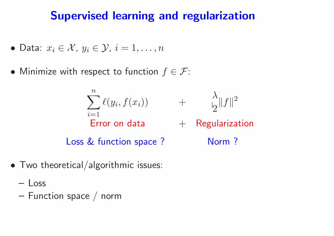
Supervised learning and regularization
• Data: xi ∈ X , yi ∈ Y, i = 1, . . . , n
• Minimize with respect to function f ∈ F :
n∑
i=1
ℓ(yi, f(xi)) +λ
2‖f‖2
Error on data + Regularization
Loss & function space ? Norm ?
• Two theoretical/algorithmic issues:
– Loss
– Function space / norm

Part II - Outline
1. Losses for particular machine learning tasks
• Classification, regression, etc...
2. Regularization by Hilbert norms (kernel methods)
• Kernels and representer theorem
• Convex duality and optimization
• Kernel design
3. Regularization by sparsity-inducing norms
• ℓ1-norm regularization
• Multiple kernel learning
• Theoretical results
• Other extensions

Losses for regression (Shawe-Taylor and Cristianini, 2004)
• Response: y ∈ R, prediction y = f(x),
– quadratic (square) loss ℓ(y, f(x)) = 12(y − f(x))2
– Not many reasons to go beyond square loss!
−3 −2 −1 0 1 2 30
1
2
3
4
y−f(x)
square
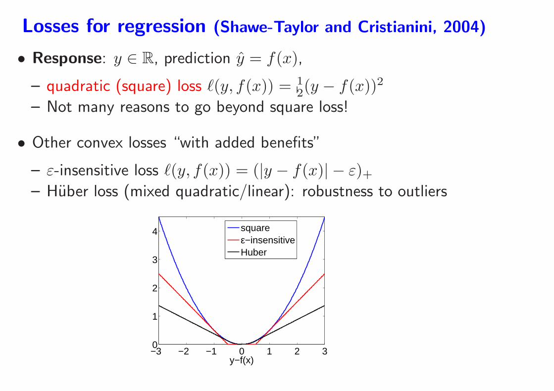
Losses for regression (Shawe-Taylor and Cristianini, 2004)
• Response: y ∈ R, prediction y = f(x),
– quadratic (square) loss ℓ(y, f(x)) = 12(y − f(x))2
– Not many reasons to go beyond square loss!
• Other convex losses “with added benefits”
– ε-insensitive loss ℓ(y, f(x)) = (|y − f(x)| − ε)+– Huber loss (mixed quadratic/linear): robustness to outliers
−3 −2 −1 0 1 2 30
1
2
3
4
y−f(x)
squareε−insensitiveHuber
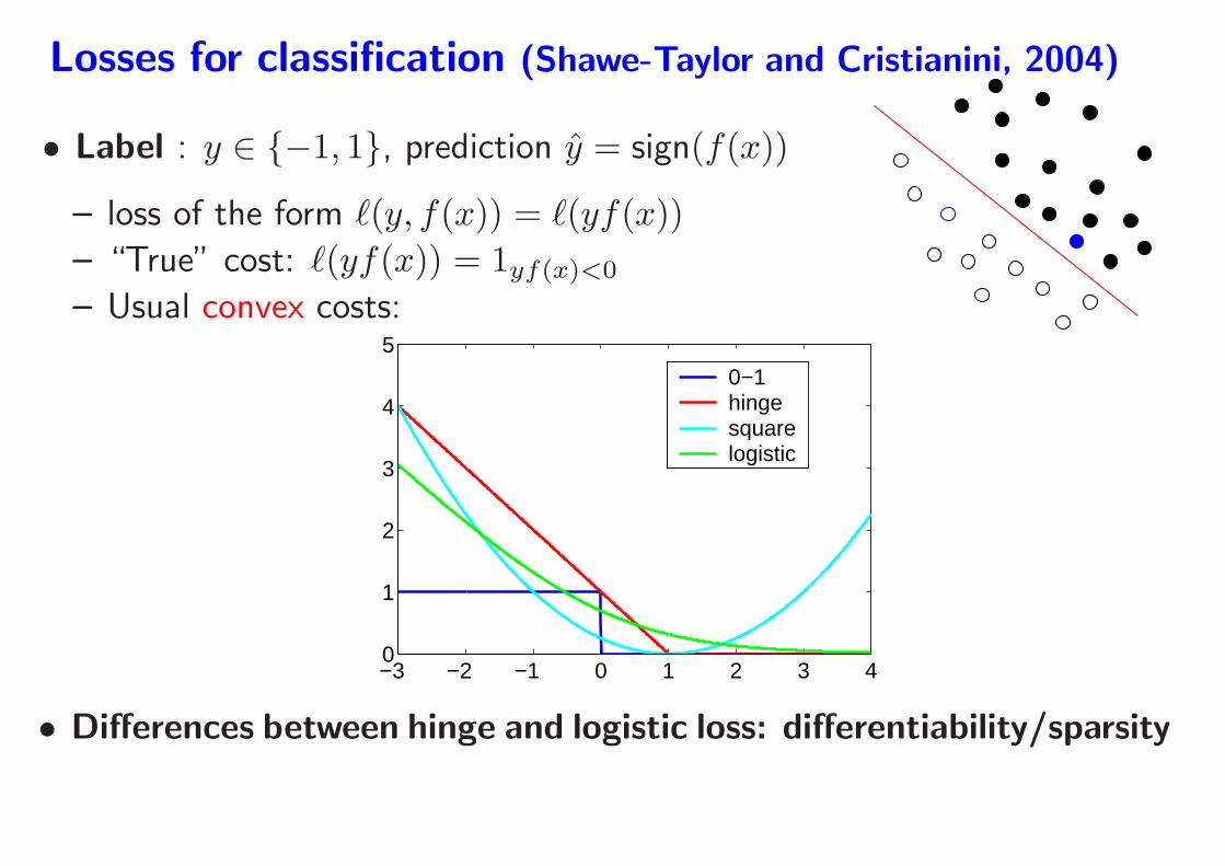
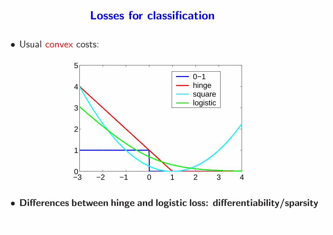
Losses for classification (Shawe-Taylor and Cristianini, 2004)
• Label : y ∈ {−1, 1}, prediction y = sign(f(x))
– loss of the form ℓ(y, f(x)) = ℓ(yf(x))
– “True” cost: ℓ(yf(x)) = 1yf(x)<0
– Usual convex costs:
−3 −2 −1 0 1 2 3 40
1
2
3
4
5
0−1hingesquarelogistic
• Differences between hinge and logistic loss: differentiability/sparsity
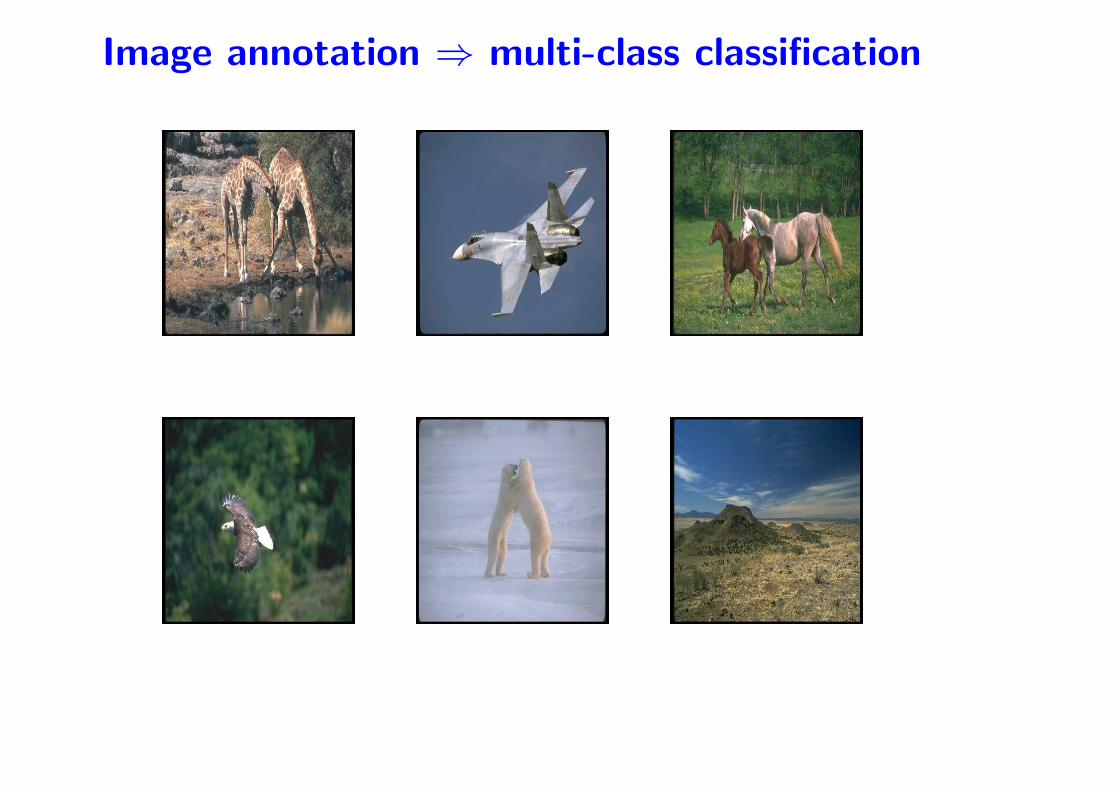
Image annotation ⇒ multi-class classification
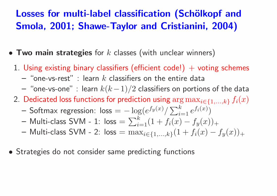
Losses for multi-label classification (Scholkopf and
Smola, 2001; Shawe-Taylor and Cristianini, 2004)
• Two main strategies for k classes (with unclear winners)
1. Using existing binary classifiers (efficient code!) + voting schemes
– “one-vs-rest” : learn k classifiers on the entire data
– “one-vs-one” : learn k(k−1)/2 classifiers on portions of the data
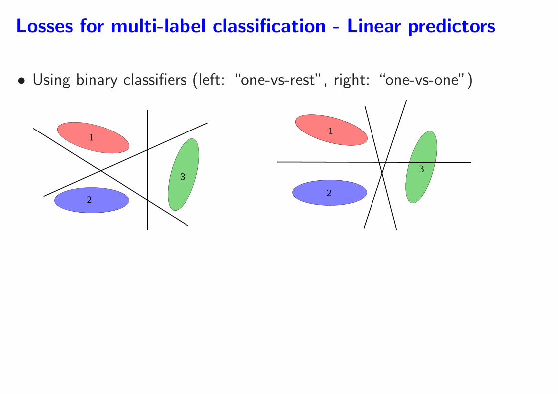
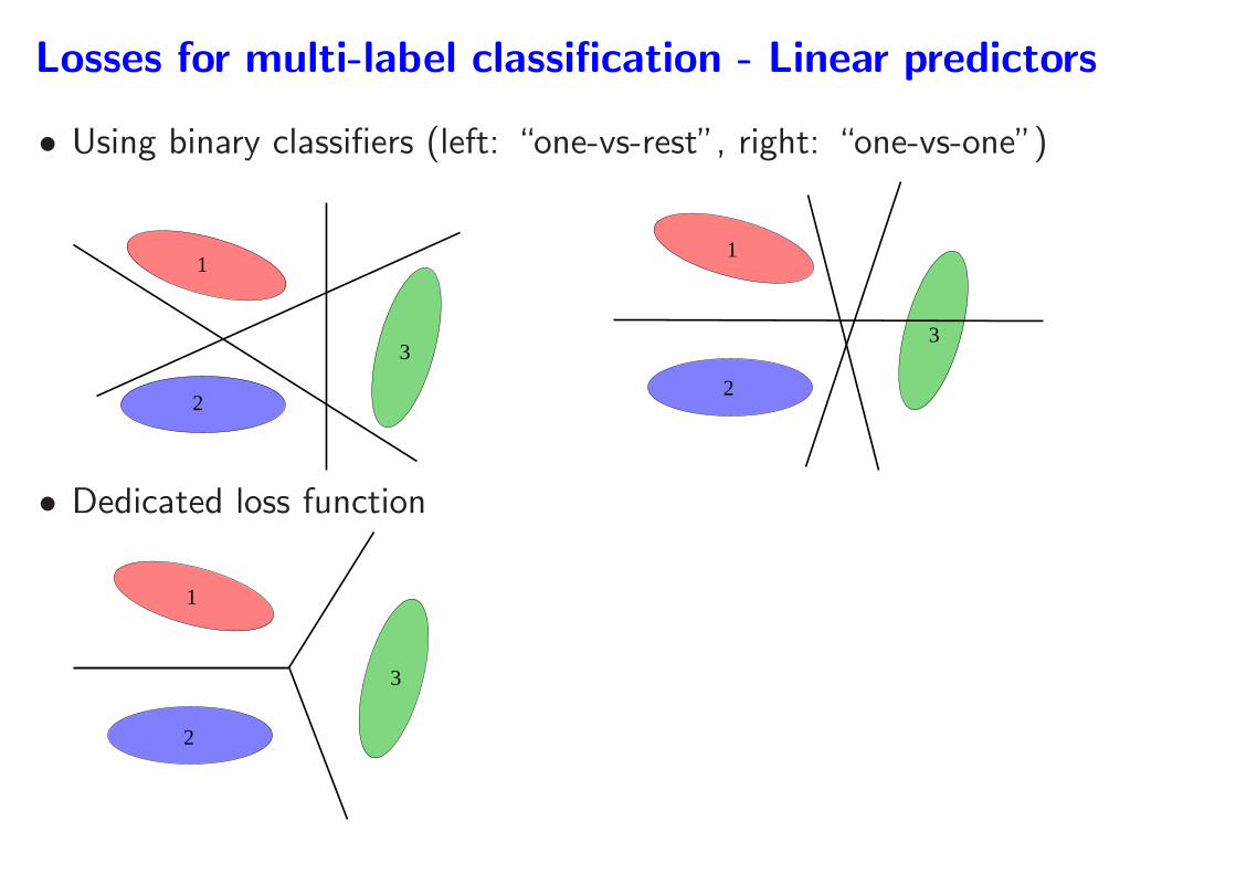
Losses for multi-label classification - Linear predictors
• Using binary classifiers (left: “one-vs-rest”, right: “one-vs-one”)
3
2
1
3
2
1
Losses for multi-label classification (Scholkopf and
Smola, 2001; Shawe-Taylor and Cristianini, 2004)
• Two main strategies for k classes (with unclear winners)
1. Using existing binary classifiers (efficient code!) + voting schemes
– “one-vs-rest” : learn k classifiers on the entire data
– “one-vs-one” : learn k(k−1)/2 classifiers on portions of the data
2. Dedicated loss functions for prediction using arg maxi∈{1,...,k} fi(x)
– Softmax regression: loss = − log(efy(x)/∑k
i=1 efi(x))
– Multi-class SVM - 1: loss =∑k
i=1(1 + fi(x)− fy(x))+– Multi-class SVM - 2: loss = maxi∈{1,...,k}(1 + fi(x)− fy(x))+
• Strategies do not consider same predicting functions
Losses for multi-label classification - Linear predictors
• Using binary classifiers (left: “one-vs-rest”, right: “one-vs-one”)
3
2
1
3
2
1
• Dedicated loss function
3
2
1
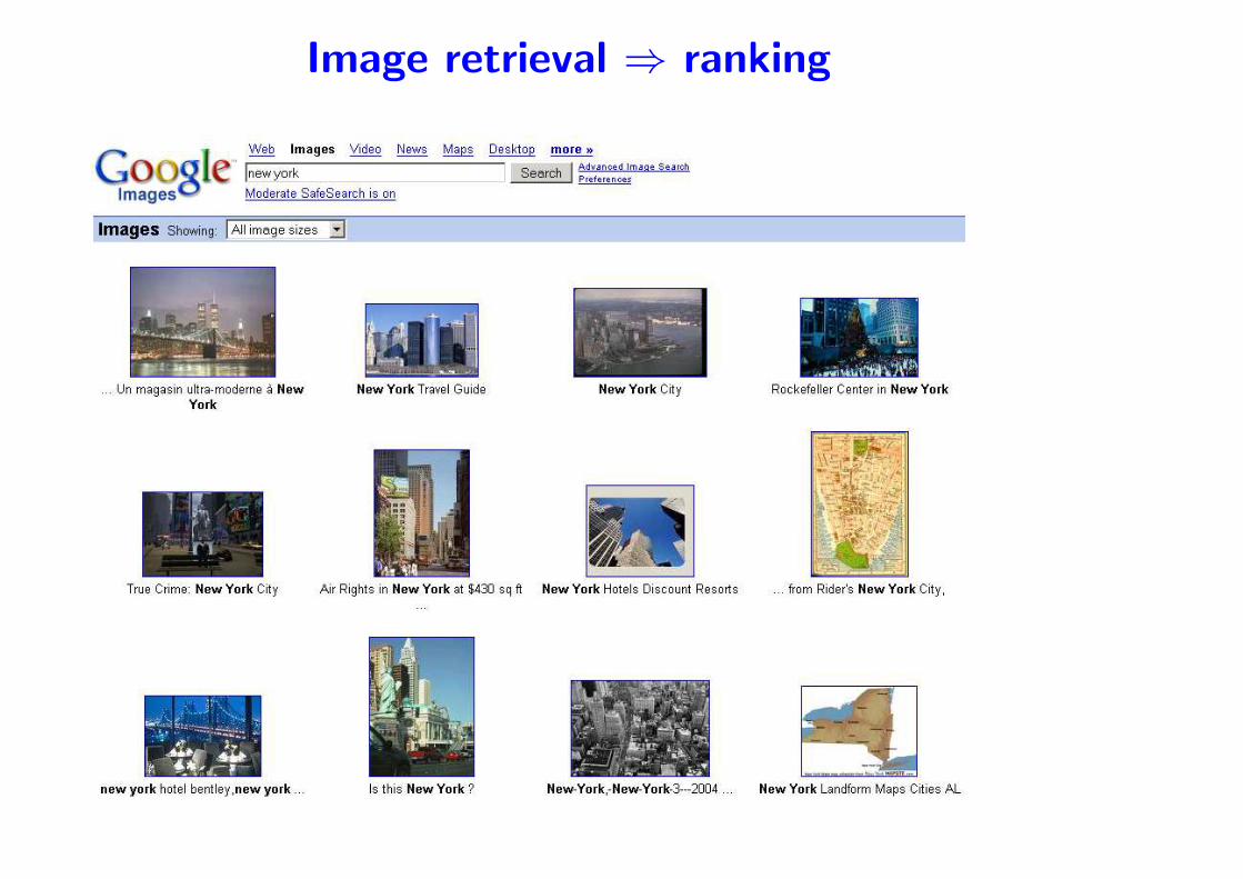
Image retrieval ⇒ ranking
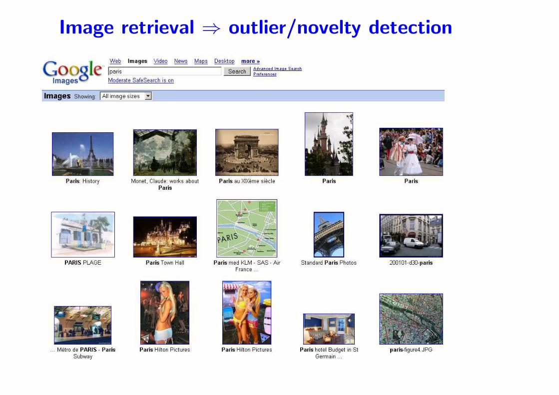
Image retrieval ⇒ outlier/novelty detection
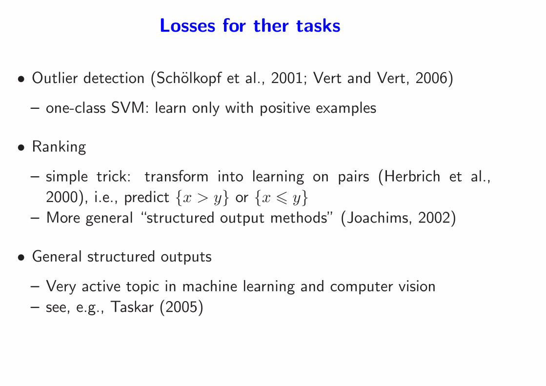
Losses for ther tasks
• Outlier detection (Scholkopf et al., 2001; Vert and Vert, 2006)
– one-class SVM: learn only with positive examples
• Ranking
– simple trick: transform into learning on pairs (Herbrich et al.,
2000), i.e., predict {x > y} or {x 6 y}
– More general “structured output methods” (Joachims, 2002)
• General structured outputs
– Very active topic in machine learning and computer vision
– see, e.g., Taskar (2005)
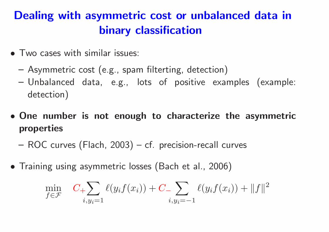
Dealing with asymmetric cost or unbalanced data in
binary classification
• Two cases with similar issues:
– Asymmetric cost (e.g., spam filterting, detection)
– Unbalanced data, e.g., lots of positive examples (example:
detection)
• One number is not enough to characterize the asymmetric
properties
– ROC curves (Flach, 2003) – cf. precision-recall curves
• Training using asymmetric losses (Bach et al., 2006)
minf∈F
C+
∑
i,yi=1
ℓ(yif(xi)) + C−
∑
i,yi=−1
ℓ(yif(xi)) + ‖f‖2

Part II - Outline
1. Losses for particular machine learning tasks
• Classification, regression, etc...
2. Regularization by Hilbert norms (kernel methods)
• Kernels and representer theorem
• Convex duality and optimization
• Kernel design
3. Regularization by sparsity-inducing norms
• ℓ1-norm regularization
• Multiple kernel learning
• Theoretical results
• Other extensions
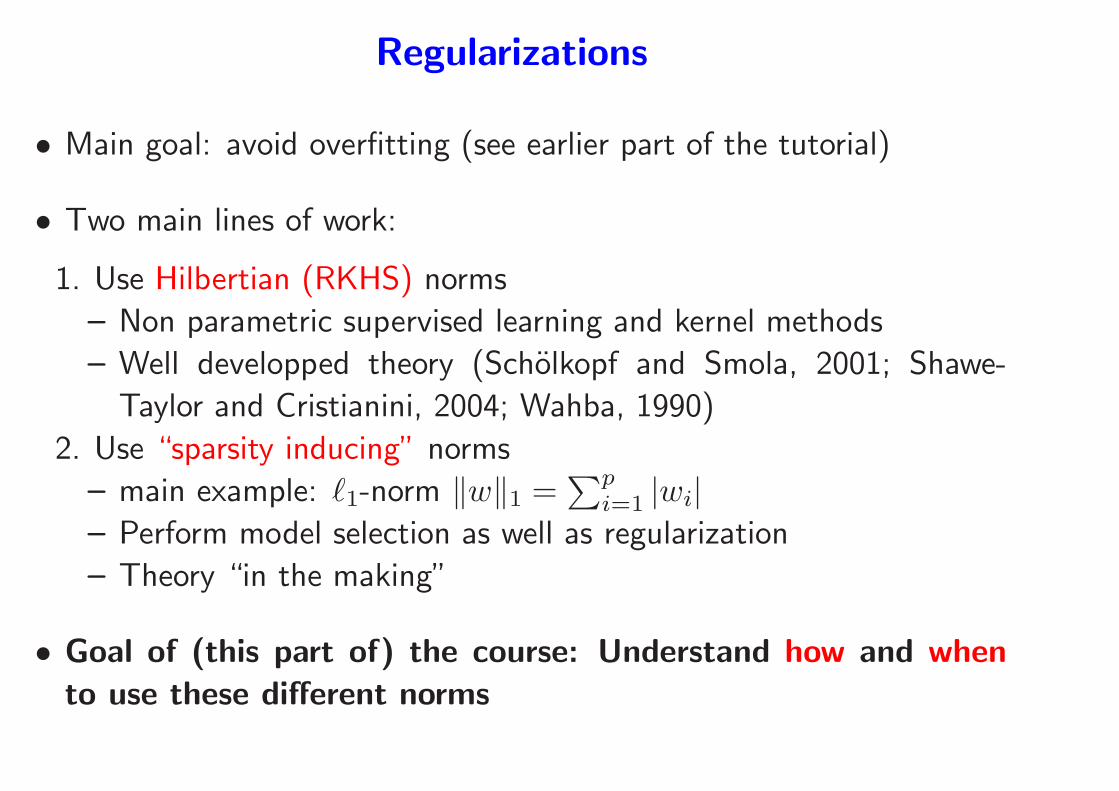
Regularizations
• Main goal: avoid overfitting (see earlier part of the tutorial)
• Two main lines of work:
1. Use Hilbertian (RKHS) norms
– Non parametric supervised learning and kernel methods
– Well developped theory (Scholkopf and Smola, 2001; Shawe-
Taylor and Cristianini, 2004; Wahba, 1990)
2. Use “sparsity inducing” norms
– main example: ℓ1-norm ‖w‖1 =∑p
i=1 |wi|
– Perform model selection as well as regularization
– Theory “in the making”
• Goal of (this part of) the course: Understand how and when
to use these different norms
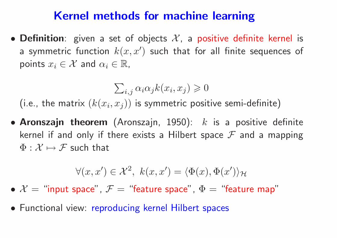
Kernel methods for machine learning
• Definition: given a set of objects X , a positive definite kernel is
a symmetric function k(x, x′) such that for all finite sequences of
points xi ∈ X and αi ∈ R,
∑
i,j αiαjk(xi, xj) > 0
(i.e., the matrix (k(xi, xj)) is symmetric positive semi-definite)
• Aronszajn theorem (Aronszajn, 1950): k is a positive definite
kernel if and only if there exists a Hilbert space F and a mapping
Φ : X 7→ F such that
∀(x, x′) ∈ X 2, k(x, x′) = 〈Φ(x),Φ(x′)〉H
• X = “input space”, F = “feature space”, Φ = “feature map”
• Functional view: reproducing kernel Hilbert spaces

Classical kernels: kernels on vectors x ∈ Rd
• Linear kernel k(x, y) = x⊤y
– Φ(x) = x
• Polynomial kernel k(x, y) = (1 + x⊤y)d
– Φ(x) = monomials
• Gaussian kernel k(x, y) = exp(−α‖x− y‖2)
– Φ(x) =??
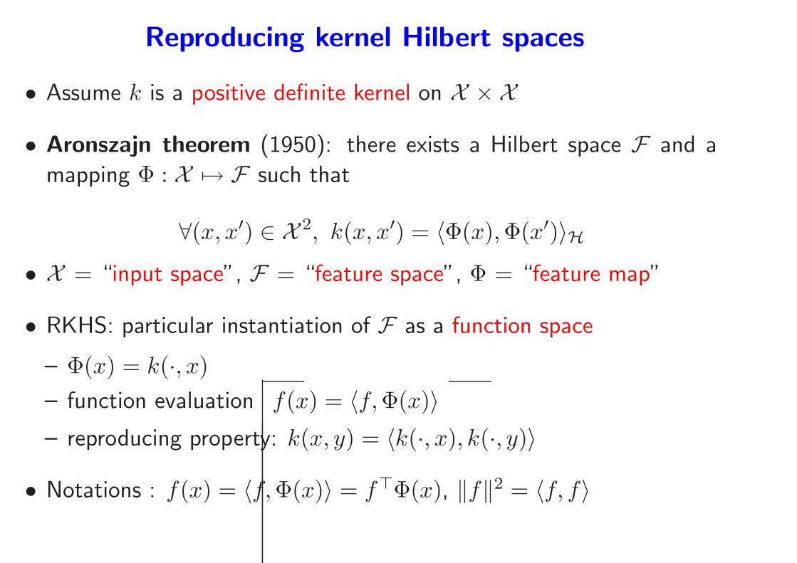
Reproducing kernel Hilbert spaces
• Assume k is a positive definite kernel on X × X
• Aronszajn theorem (1950): there exists a Hilbert space F and a
mapping Φ : X 7→ F such that
∀(x, x′) ∈ X 2, k(x, x′) = 〈Φ(x),Φ(x′)〉H
• X = “input space”, F = “feature space”, Φ = “feature map”
• RKHS: particular instantiation of F as a function space
– Φ(x) = k(·, x)
– function evaluation f(x) = 〈f,Φ(x)〉
– reproducing property: k(x, y) = 〈k(·, x), k(·, y)〉
• Notations : f(x) = 〈f,Φ(x)〉 = f⊤Φ(x), ‖f‖2 = 〈f, f〉
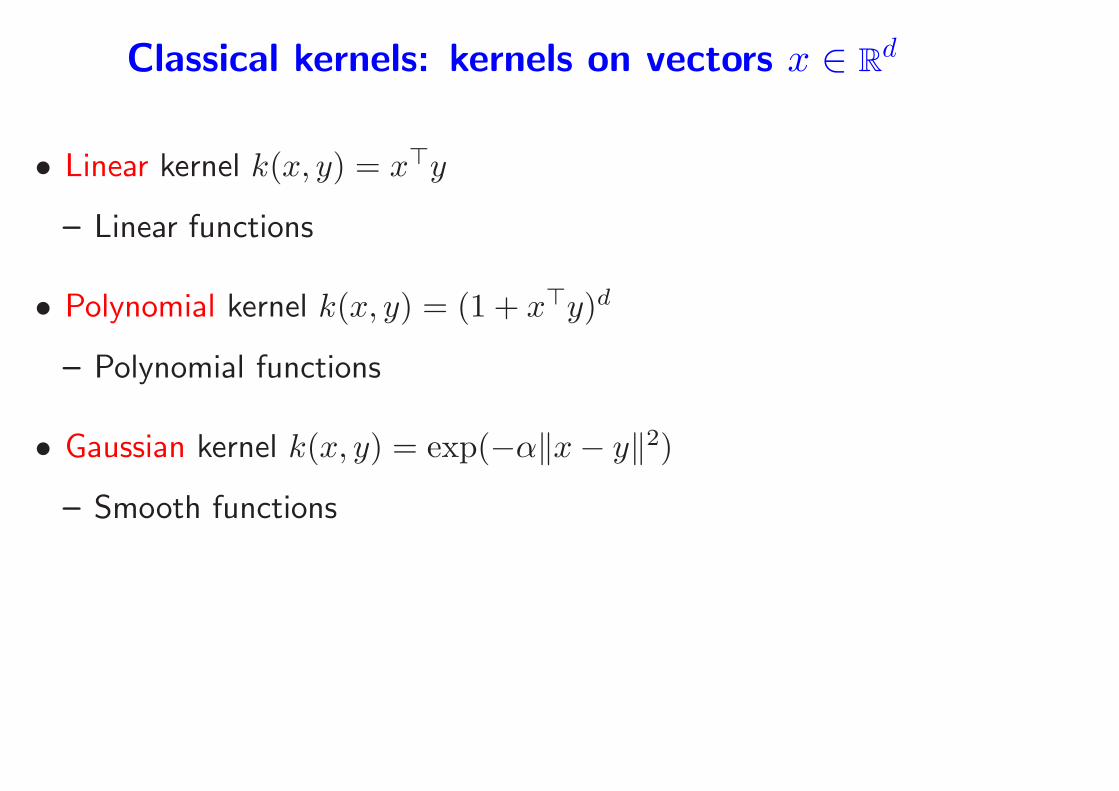
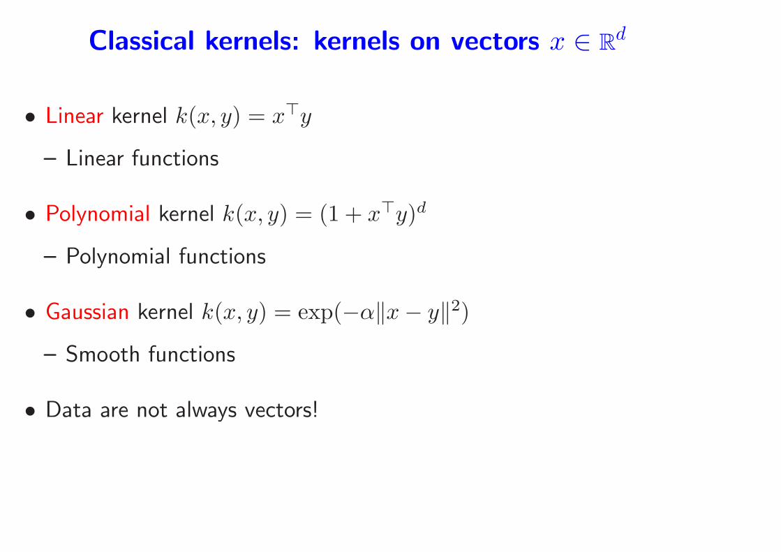
Classical kernels: kernels on vectors x ∈ Rd
• Linear kernel k(x, y) = x⊤y
– Linear functions
• Polynomial kernel k(x, y) = (1 + x⊤y)d
– Polynomial functions
• Gaussian kernel k(x, y) = exp(−α‖x− y‖2)
– Smooth functions
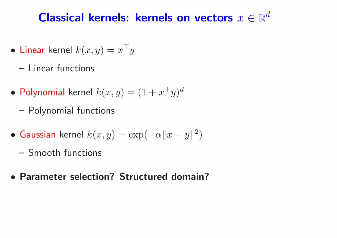
Classical kernels: kernels on vectors x ∈ Rd
• Linear kernel k(x, y) = x⊤y
– Linear functions
• Polynomial kernel k(x, y) = (1 + x⊤y)d
– Polynomial functions
• Gaussian kernel k(x, y) = exp(−α‖x− y‖2)
– Smooth functions
• Parameter selection? Structured domain?
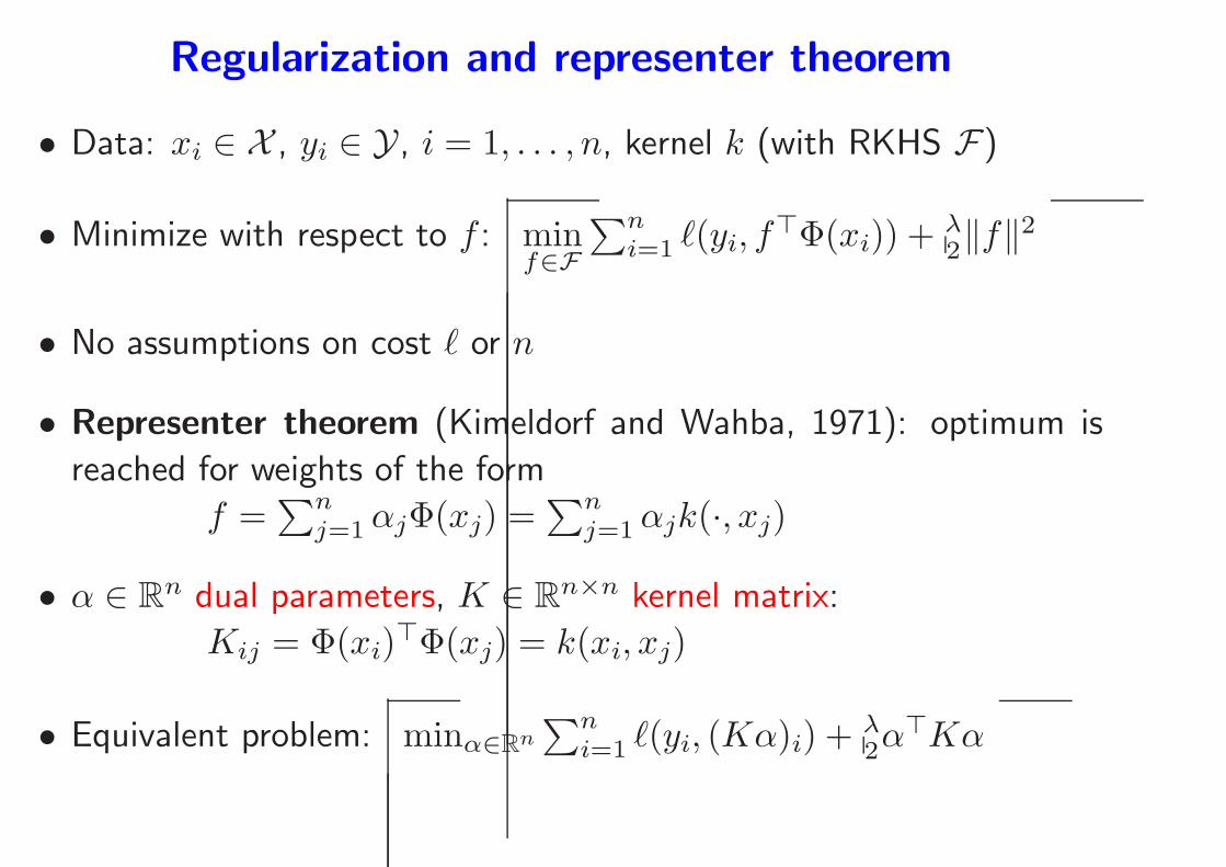
Regularization and representer theorem
• Data: xi ∈ X , yi ∈ Y, i = 1, . . . , n, kernel k (with RKHS F)
• Minimize with respect to f : minf∈F
∑ni=1 ℓ(yi, f
⊤Φ(xi)) + λ2‖f‖
2
• No assumptions on cost ℓ or n
• Representer theorem (Kimeldorf and Wahba, 1971): optimum is
reached for weights of the form
f =∑n
j=1αjΦ(xj) =∑n
j=1αjk(·, xj)
• α ∈ Rn dual parameters, K ∈ R
n×n kernel matrix:
Kij = Φ(xi)⊤Φ(xj) = k(xi, xj)
• Equivalent problem: minα∈Rn∑n
i=1 ℓ(yi, (Kα)i) + λ2α
⊤Kα
Kernel trick and modularity
• Kernel trick: any algorithm for finite-dimensional vectors that only
uses pairwise dot-products can be applied in the feature space.
– Replacing dot-products by kernel functions
– Implicit use of (very) large feature spaces
– Linear to non-linear learning methods
Kernel trick and modularity
• Kernel trick: any algorithm for finite-dimensional vectors that only
uses pairwise dot-products can be applied in the feature space.
– Replacing dot-products by kernel functions
– Implicit use of (very) large feature spaces
– Linear to non-linear learning methods
• Modularity of kernel methods
1. Work on new algorithms and theoretical analysis
2. Work on new kernels for specific data types
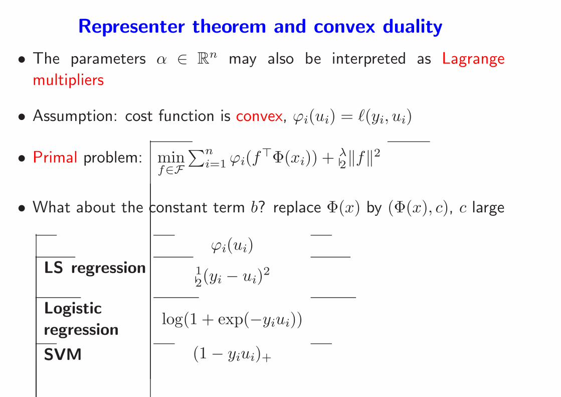
Representer theorem and convex duality
• The parameters α ∈ Rn may also be interpreted as Lagrange
multipliers
• Assumption: cost function is convex, ϕi(ui) = ℓ(yi, ui)
• Primal problem: minf∈F
∑ni=1ϕi(f
⊤Φ(xi)) + λ2‖f‖
2
• What about the constant term b? replace Φ(x) by (Φ(x), c), c large
ϕi(ui)
LS regression 12(yi − ui)
2
Logistic
regressionlog(1 + exp(−yiui))
SVM (1− yiui)+

Representer theorem and convex duality
Proof
• Primal problem: minf∈F
∑ni=1ϕi(f
⊤Φ(xi)) + λ2‖f‖
2
• Define ψi(vi) = maxui∈R
viui − ϕi(ui) as the Fenchel conjugate of ϕi
• Main trick: introduce constraint ui = f⊤Φ(xi) and associated
Lagrange multipliers αi
• Lagrangian L(α, f) =n∑
i=1
ϕi(ui) +λ
2‖f‖2 + λ
n∑
i=1
αi(ui − f⊤Φ(xi))
– Maximize with respect to ui ⇒ term of the form −ψi(−λαi)
– Maximize with respect to f ⇒ f =∑n
i=1αiΦ(xi)
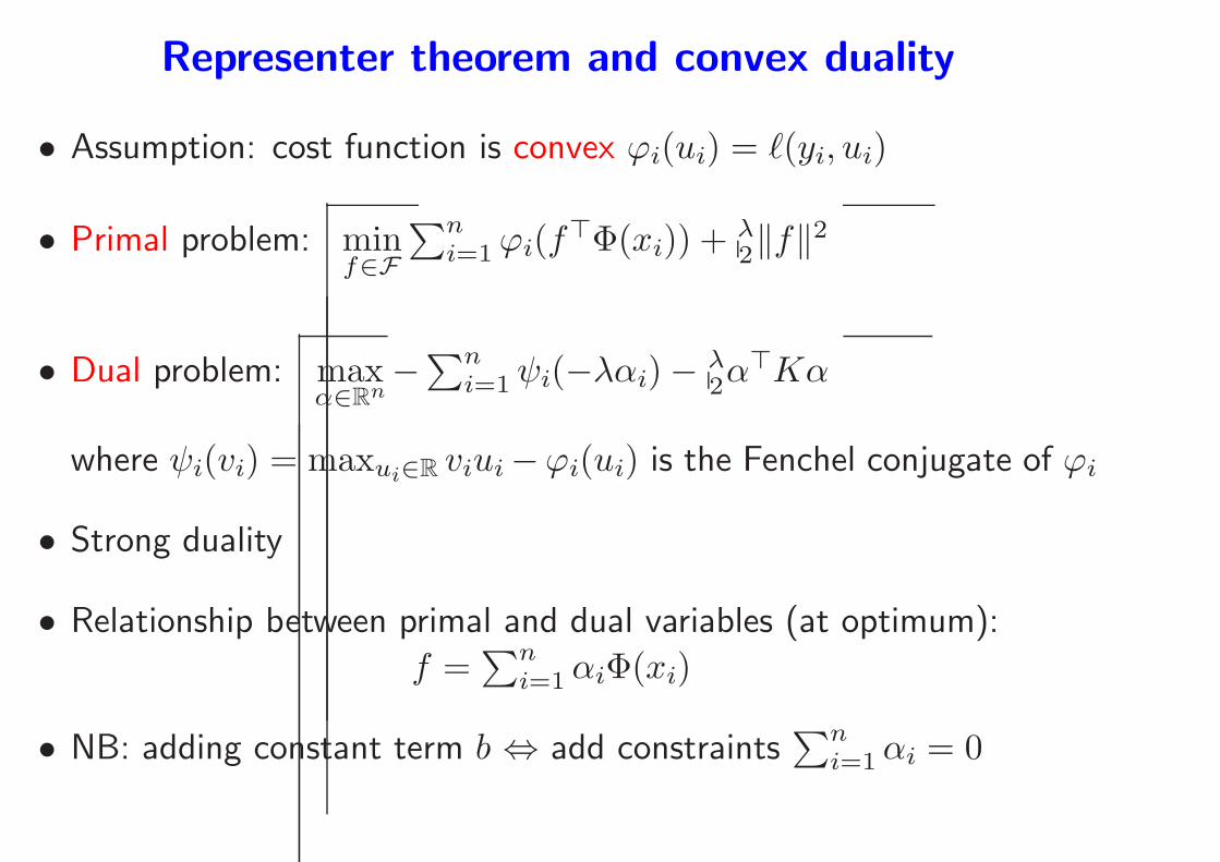
Representer theorem and convex duality
• Assumption: cost function is convex ϕi(ui) = ℓ(yi, ui)
• Primal problem: minf∈F
∑ni=1ϕi(f
⊤Φ(xi)) + λ2‖f‖
2
• Dual problem: maxα∈Rn
−∑n
i=1ψi(−λαi)−λ2α
⊤Kα
where ψi(vi) = maxui∈R viui−ϕi(ui) is the Fenchel conjugate of ϕi
• Strong duality
• Relationship between primal and dual variables (at optimum):
f =∑n
i=1αiΦ(xi)
• NB: adding constant term b ⇔ add constraints∑n
i=1αi = 0
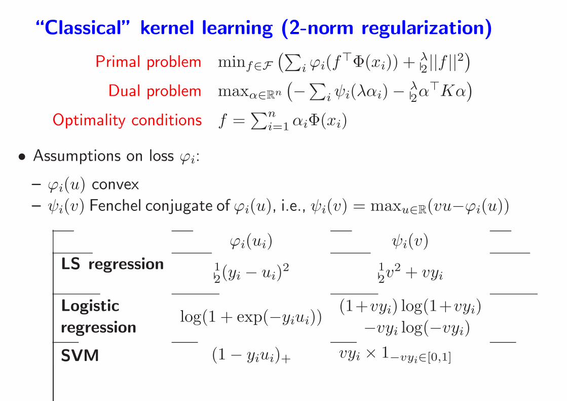
“Classical” kernel learning (2-norm regularization)
Primal problem minf∈F
(∑
iϕi(f⊤Φ(xi)) + λ
2 ||f ||2)
Dual problem maxα∈Rn
(
−∑
iψi(λαi)−λ2α
⊤Kα)
Optimality conditions f =∑n
i=1αiΦ(xi)
• Assumptions on loss ϕi:
– ϕi(u) convex
– ψi(v) Fenchel conjugate of ϕi(u), i.e., ψi(v) = maxu∈R(vu−ϕi(u))
ϕi(ui) ψi(v)
LS regression 12(yi − ui)
2 12v
2 + vyi
Logistic
regressionlog(1 + exp(−yiui))
(1+vyi) log(1+vyi)
−vyi log(−vyi)
SVM (1− yiui)+ vyi × 1−vyi∈[0,1]
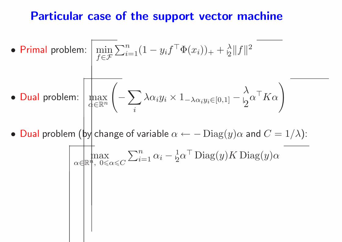
Particular case of the support vector machine
• Primal problem: minf∈F
∑ni=1(1− yif
⊤Φ(xi))+ + λ2‖f‖
2
• Dual problem: maxα∈Rn
(
−∑
i
λαiyi × 1−λαiyi∈[0,1] −λ
2α⊤Kα
)
• Dual problem (by change of variable α← −Diag(y)α and C = 1/λ):
maxα∈Rn, 06α6C
∑ni=1αi −
12α
⊤ Diag(y)K Diag(y)α
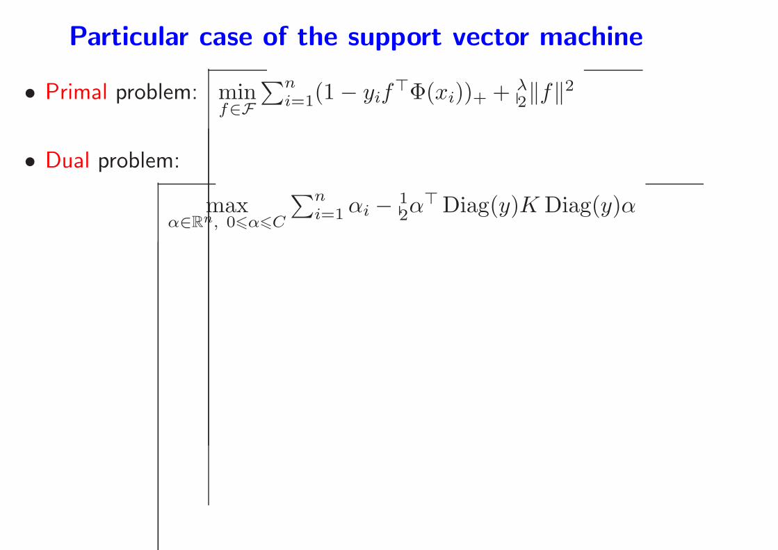
Particular case of the support vector machine
• Primal problem: minf∈F
∑ni=1(1− yif
⊤Φ(xi))+ + λ2‖f‖
2
• Dual problem:
maxα∈Rn, 06α6C
∑ni=1αi −
12α
⊤ Diag(y)K Diag(y)α
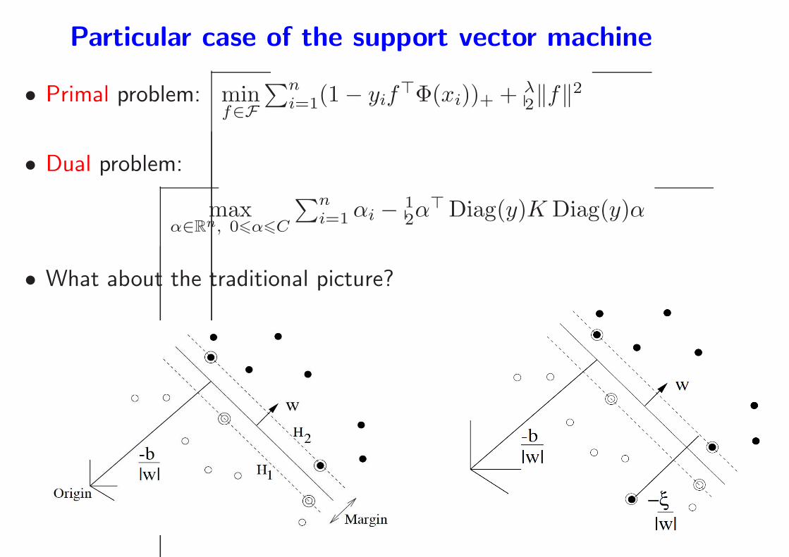
Particular case of the support vector machine
• Primal problem: minf∈F
∑ni=1(1− yif
⊤Φ(xi))+ + λ2‖f‖
2
• Dual problem:
maxα∈Rn, 06α6C
∑ni=1αi −
12α
⊤ Diag(y)K Diag(y)α
• What about the traditional picture?
Losses for classification
• Usual convex costs:
−3 −2 −1 0 1 2 3 40
1
2
3
4
5
0−1hingesquarelogistic
• Differences between hinge and logistic loss: differentiability/sparsity
Support vector machine or logistic regression?
• Predictive performance is similar
• Only true difference is numerical
– SVM: sparsity in α
– Logistic: differentiable loss function
• Which one to use?
– Linear kernel ⇒ Logistic + Newton/Gradient descent
– Nonlinear kernel ⇒ SVM + dual methods or simpleSVM
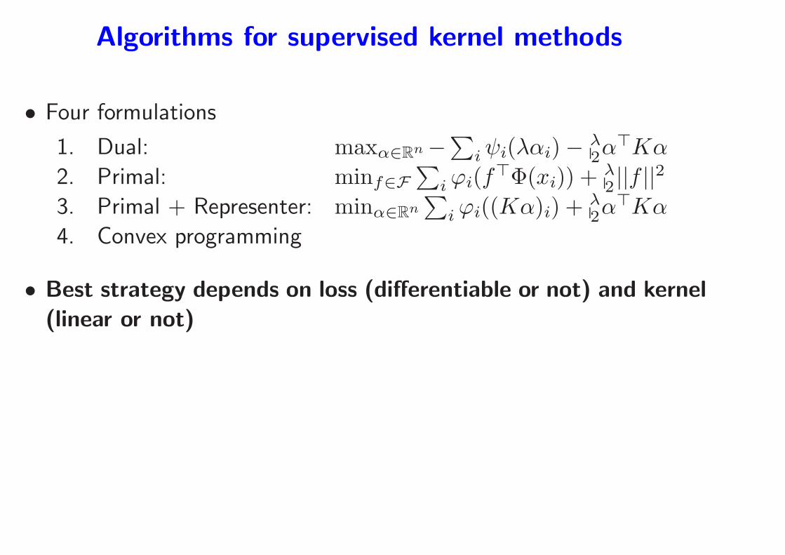
Algorithms for supervised kernel methods
• Four formulations
1. Dual: maxα∈Rn−∑
iψi(λαi)−λ2α
⊤Kα
2. Primal: minf∈F
∑
iϕi(f⊤Φ(xi)) + λ
2 ||f ||2
3. Primal + Representer: minα∈Rn∑
iϕi((Kα)i) + λ2α
⊤Kα
4. Convex programming
• Best strategy depends on loss (differentiable or not) and kernel
(linear or not)
Dual methods
• Dual problem: maxα∈Rn−∑
iψi(λαi)−λ2α
⊤Kα
• Main method: coordinate descent (a.k.a. sequential minimal
optimization - SMO) (Platt, 1998; Bottou and Lin, 2007; Joachims,
1998)
– Efficient when loss is piecewise quadratic (i.e., hinge = SVM)
– Sparsity may be used in the case of the SVM
• Computational complexity: between quadratic and cubic in n
• Works for all kernels
Primal methods
• Primal problem: minf∈F
∑
iϕi(f⊤Φ(xi)) + λ
2 ||f ||2
• Only works directly if Φ(x) may be built explicitly and has small
dimension
– Example: linear kernel in small dimensions
• Differentiable loss: gradient descent or Newton’s method are very
efficient in small dimensions
• Larger scale: stochastic gradient descent (Shalev-Shwartz et al.,
2007; Bottou and Bousquet, 2008)
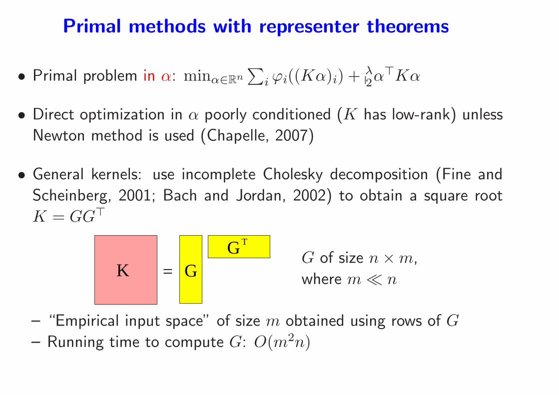
Primal methods with representer theorems
• Primal problem in α: minα∈Rn∑
iϕi((Kα)i) + λ2α
⊤Kα
• Direct optimization in α poorly conditioned (K has low-rank) unless
Newton method is used (Chapelle, 2007)
• General kernels: use incomplete Cholesky decomposition (Fine and
Scheinberg, 2001; Bach and Jordan, 2002) to obtain a square root
K = GG⊤
K
T
=G
GG of size n×m,
where m≪ n
– “Empirical input space” of size m obtained using rows of G
– Running time to compute G: O(m2n)
Direct convex programming
• Convex programming toolboxes ⇒ very inefficient!
• May use special structure of the problem
– e.g., SVM and sparsity in α
• Active set method for the SVM: SimpleSVM (Vishwanathan et al.,
2003; Loosli et al., 2005)
– Cubic complexity in the number of support vectors
• Full regularization path for the SVM (Hastie et al., 2005; Bach et al.,
2006)
– Cubic complexity in the number of support vectors
– May be extended to other settings (Rosset and Zhu, 2007)

Part II - Outline
1. Losses for particular machine learning tasks
• Classification, regression, etc...
2. Regularization by Hilbert norms (kernel methods)
• Kernels and representer theorem
• Convex duality and optimization
• Kernel design
3. Regularization by sparsity-inducing norms
• ℓ1-norm regularization
• Multiple kernel learning
• Theoretical results
• Other extensions
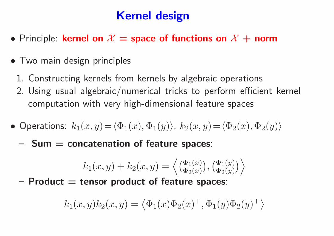
Kernel design
• Principle: kernel on X = space of functions on X + norm
• Two main design principles
1. Constructing kernels from kernels by algebraic operations
2. Using usual algebraic/numerical tricks to perform efficient kernel
computation with very high-dimensional feature spaces
• Operations: k1(x, y)=〈Φ1(x),Φ1(y)〉, k2(x, y)=〈Φ2(x),Φ2(y)〉
– Sum = concatenation of feature spaces:
k1(x, y) + k2(x, y) =⟨
(Φ1(x)Φ2(x)
)
,(Φ1(y)Φ2(y)
)
⟩
– Product = tensor product of feature spaces:
k1(x, y)k2(x, y) =⟨
Φ1(x)Φ2(x)⊤,Φ1(y)Φ2(y)
⊤⟩
Classical kernels: kernels on vectors x ∈ Rd
• Linear kernel k(x, y) = x⊤y
– Linear functions
• Polynomial kernel k(x, y) = (1 + x⊤y)d
– Polynomial functions
• Gaussian kernel k(x, y) = exp(−α‖x− y‖2)
– Smooth functions
• Data are not always vectors!
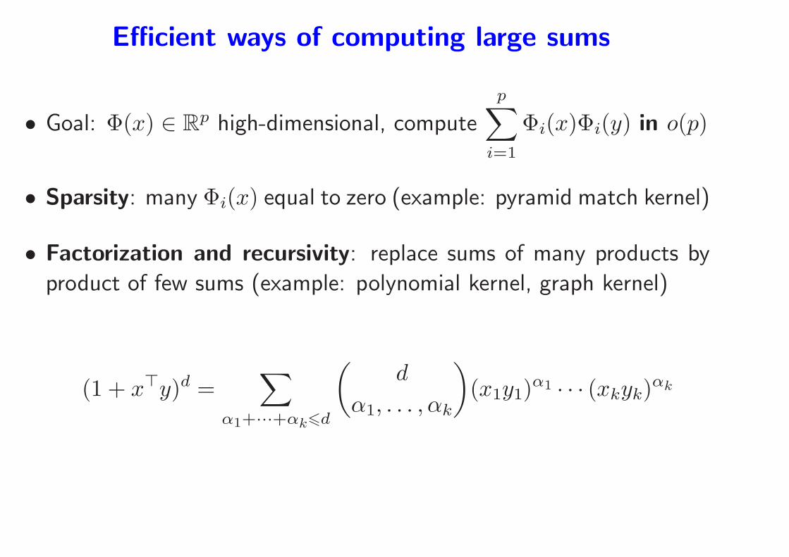
Efficient ways of computing large sums
• Goal: Φ(x) ∈ Rp high-dimensional, compute
p∑
i=1
Φi(x)Φi(y) in o(p)
• Sparsity: many Φi(x) equal to zero (example: pyramid match kernel)
• Factorization and recursivity: replace sums of many products by
product of few sums (example: polynomial kernel, graph kernel)
(1 + x⊤y)d =∑
α1+···+αk6d
(
d
α1, . . . , αk
)
(x1y1)α1 · · · (xkyk)
αk
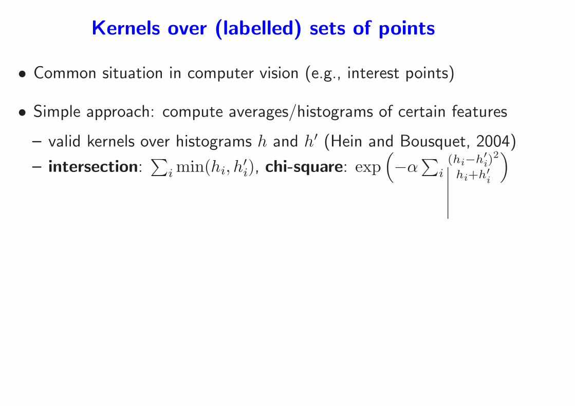
Kernels over (labelled) sets of points
• Common situation in computer vision (e.g., interest points)
• Simple approach: compute averages/histograms of certain features
– valid kernels over histograms h and h′ (Hein and Bousquet, 2004)
– intersection:∑
i min(hi, h′i), chi-square: exp
(
−α∑
i(hi−h′
i)2
hi+h′i
)
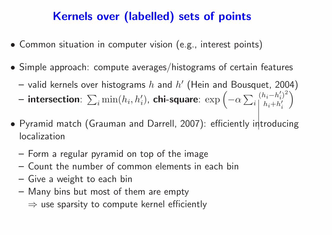
• Pyramid match (Grauman and Darrell, 2007): efficiently introducing
localization
– Form a regular pyramid on top of the image
– Count the number of common elements in each bin
– Give a weight to each bin
– Many bins but most of them are empty
⇒ use sparsity to compute kernel efficiently
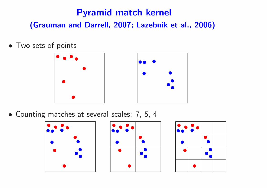
Pyramid match kernel
(Grauman and Darrell, 2007; Lazebnik et al., 2006)
• Two sets of points
• Counting matches at several scales: 7, 5, 4
Kernels from segmentation graphs
• Goal of segmentation: extract objects of interest
• Many methods available, ....
– ... but, rarely find the object of interest entirely
• Segmentation graphs
– Allows to work on “more reliable” over-segmentation
– Going to a large square grid (millions of pixels) to a small graph
(dozens or hundreds of regions)
• How to build a kernel over segmenation graphs?
– NB: more generally, kernelizing existing representations?
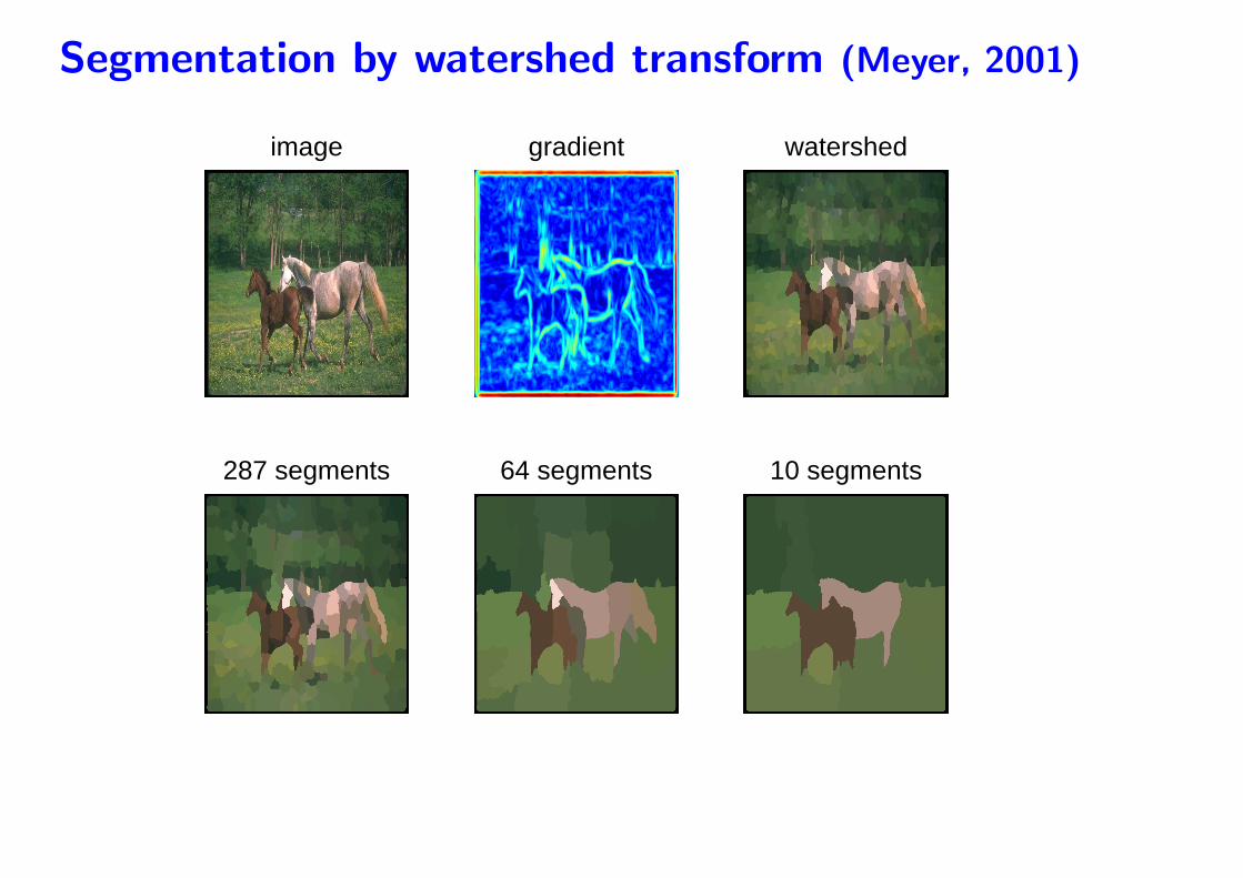
Segmentation by watershed transform (Meyer, 2001)
image gradient watershed
287 segments 64 segments 10 segments
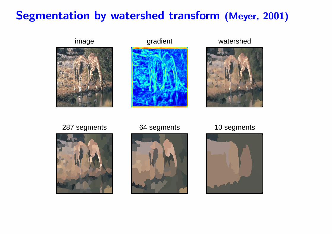
Segmentation by watershed transform (Meyer, 2001)
image gradient watershed
287 segments 64 segments 10 segments
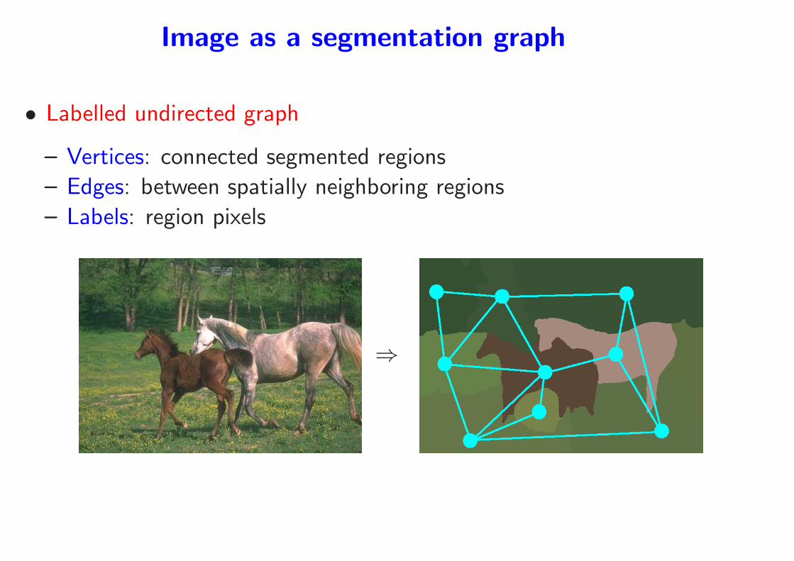
Image as a segmentation graph
• Labelled undirected graph
– Vertices: connected segmented regions
– Edges: between spatially neighboring regions
– Labels: region pixels
⇒
Image as a segmentation graph
• Labelled undirected graph
– Vertices: connected segmented regions
– Edges: between spatially neighboring regions
– Labels: region pixels
• Difficulties
– Extremely high-dimensional labels
– Planar undirected graph
– Inexact matching
• Graph kernels (Gartner et al., 2003; Kashima et al., 2004; Harchaoui
and Bach, 2007) provide an elegant and efficient solution
Kernels between structured objects
Strings, graphs, etc... (Shawe-Taylor and Cristianini, 2004)
• Numerous applications (text, bio-informatics, speech, vision)
• Common design principle: enumeration of subparts (Haussler,
1999; Watkins, 1999)
– Efficient for strings
– Possibility of gaps, partial matches, very efficient algorithms
• Most approaches fails for general graphs (even for undirected trees!)
– NP-Hardness results (Ramon and Gartner, 2003)
– Need specific set of subparts
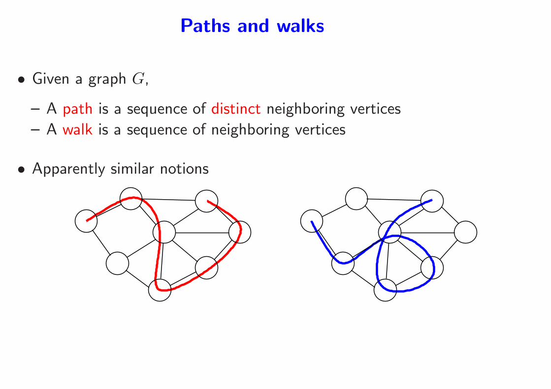
Paths and walks
• Given a graph G,
– A path is a sequence of distinct neighboring vertices
– A walk is a sequence of neighboring vertices
• Apparently similar notions
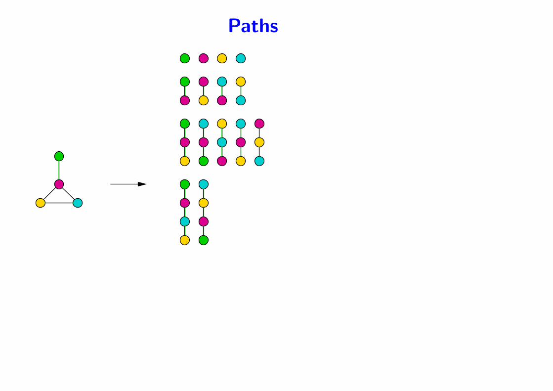
Paths
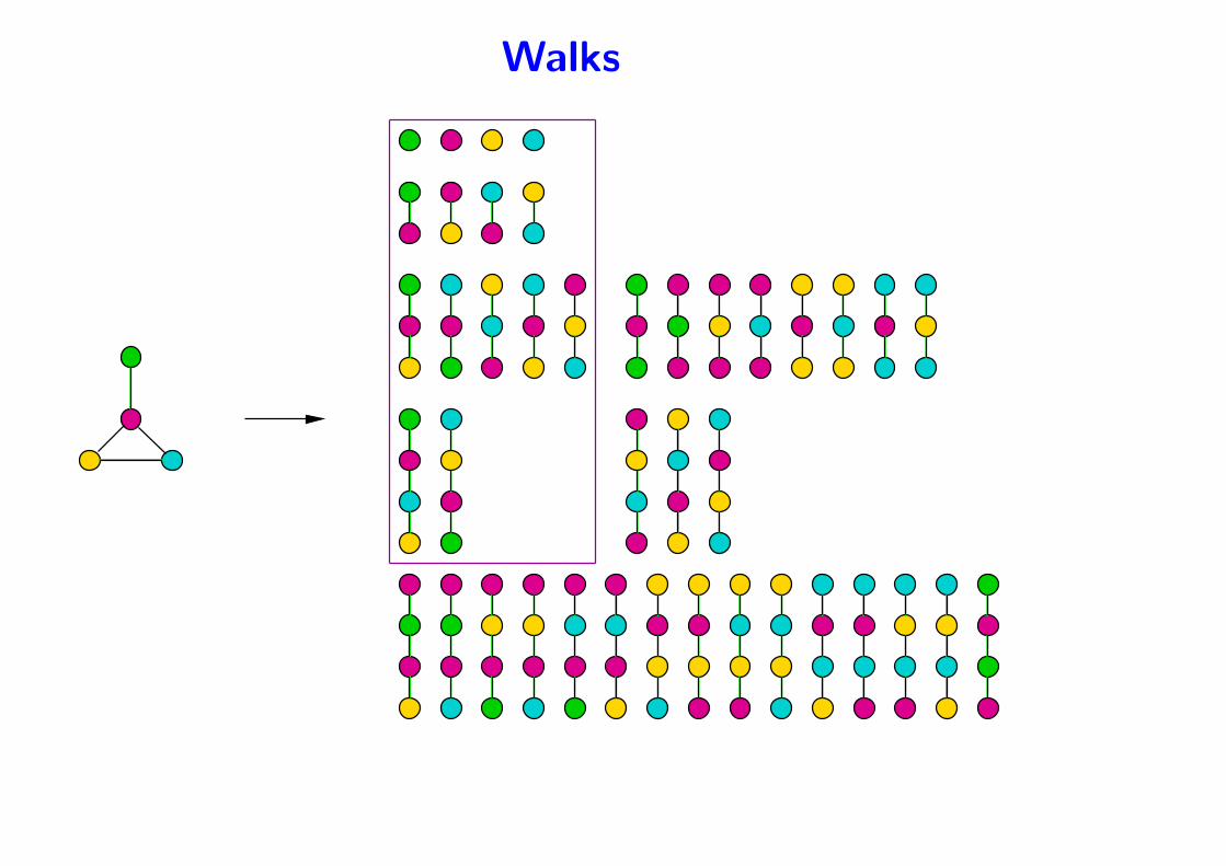
Walks
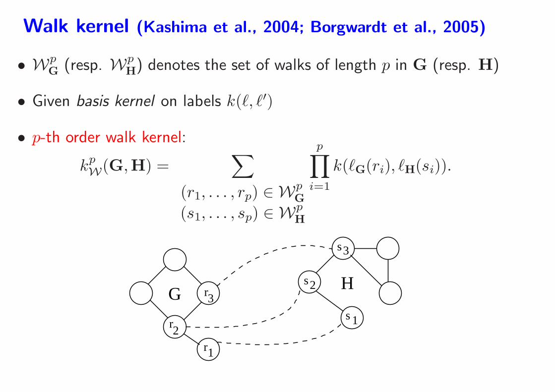
Walk kernel (Kashima et al., 2004; Borgwardt et al., 2005)
• WpG
(resp. WpH) denotes the set of walks of length p in G (resp. H)
• Given basis kernel on labels k(ℓ, ℓ′)
• p-th order walk kernel:
kpW(G,H) =
∑
(r1, . . . , rp) ∈ WpG
(s1, . . . , sp) ∈ WpH
p∏
i=1
k(ℓG(ri), ℓH(si)).
G
1
s3
2s
s 1r2
3rH
r
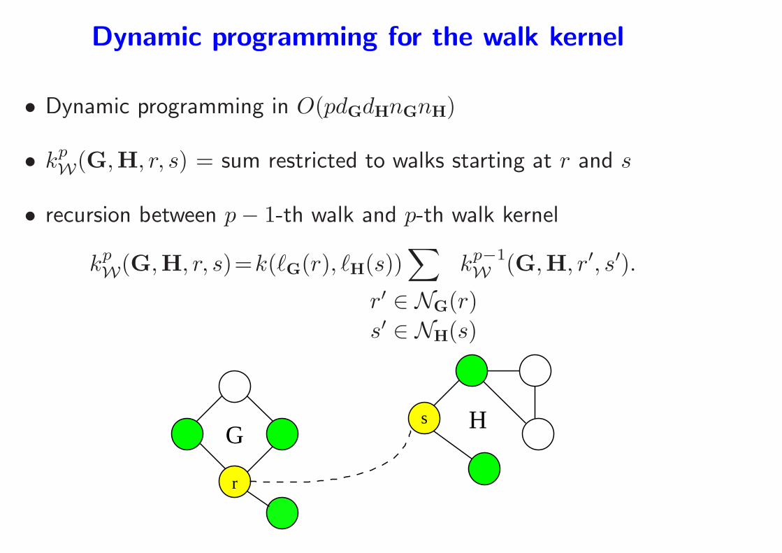
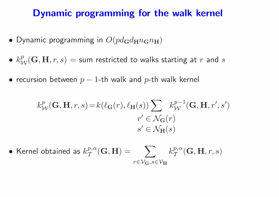
Dynamic programming for the walk kernel
• Dynamic programming in O(pdGdHnGnH)
• kpW(G,H, r, s) = sum restricted to walks starting at r and s
• recursion between p− 1-th walk and p-th walk kernel
kpW(G,H, r, s)=k(ℓG(r), ℓH(s))
∑
r′ ∈ NG(r)
s′ ∈ NH(s)
kp−1W (G,H, r′, s′).
Gs
r
H
Dynamic programming for the walk kernel
• Dynamic programming in O(pdGdHnGnH)
• kpW(G,H, r, s) = sum restricted to walks starting at r and s
• recursion between p− 1-th walk and p-th walk kernel
kpW(G,H, r, s)=k(ℓG(r), ℓH(s))
∑
r′ ∈ NG(r)
s′ ∈ NH(s)
kp−1W (G,H, r′, s′)
• Kernel obtained as kp,αT (G,H) =
∑
r∈VG,s∈VH
kp,αT (G,H, r, s)
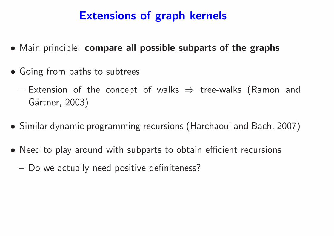
Extensions of graph kernels
• Main principle: compare all possible subparts of the graphs
• Going from paths to subtrees
– Extension of the concept of walks ⇒ tree-walks (Ramon and
Gartner, 2003)
• Similar dynamic programming recursions (Harchaoui and Bach, 2007)
• Need to play around with subparts to obtain efficient recursions
– Do we actually need positive definiteness?

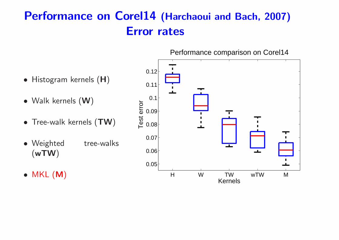
Performance on Corel14 (Harchaoui and Bach, 2007)
• Corel14: 1400 natural images with 14 classes
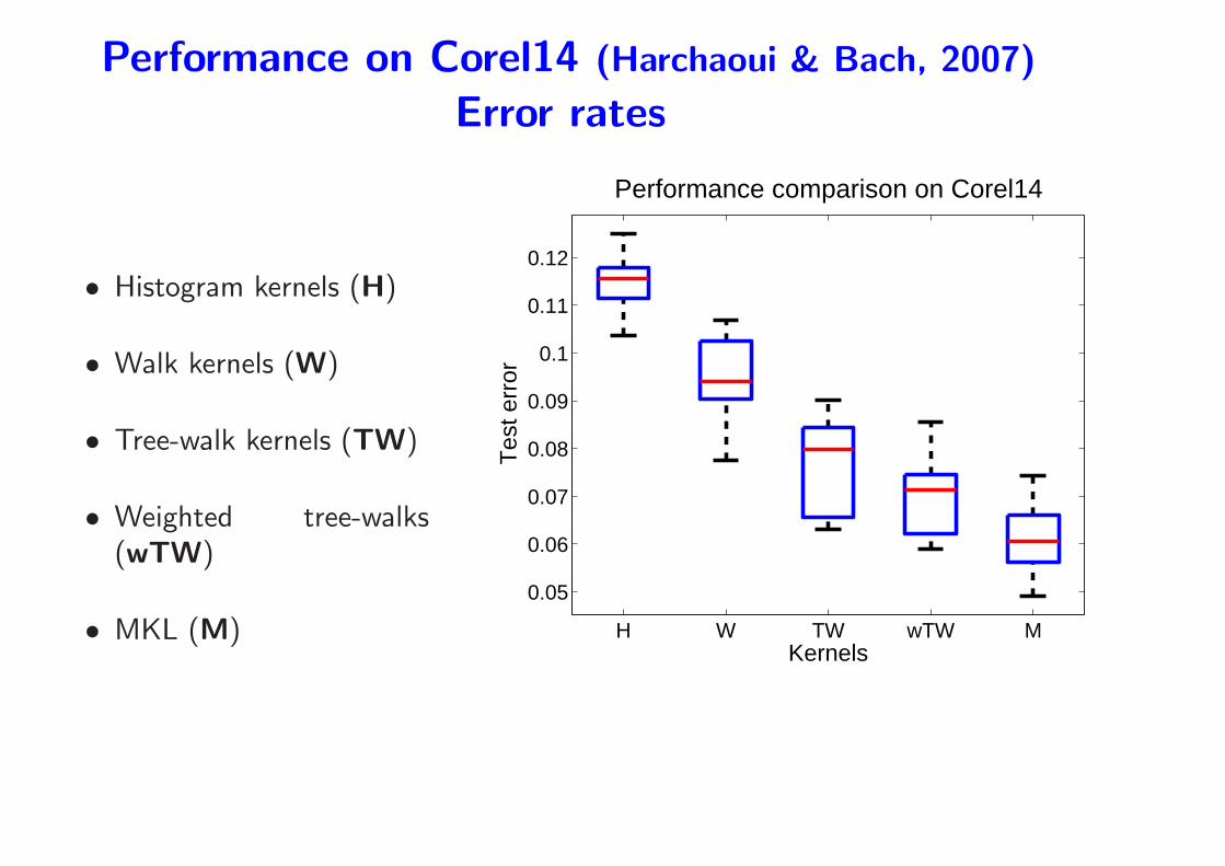
Performance on Corel14 (Harchaoui & Bach, 2007)
Error rates
• Histogram kernels (H)
• Walk kernels (W)
• Tree-walk kernels (TW)
• Weighted tree-walks(wTW)
• MKL (M) H W TW wTW M
0.05
0.06
0.07
0.08
0.09
0.1
0.11
0.12
Tes
t err
or
Kernels
Performance comparison on Corel14
Kernel methods - Summary
• Kernels and representer theorems
– Clear distinction between representation/algorithms
• Algorithms
– Two formulations (primal/dual)
– Logistic or SVM?
• Kernel design
– Very large feature spaces with efficient kernel evaluations
Part II - Outline
1. Losses for particular machine learning tasks
• Classification, regression, etc...
2. Regularization by Hilbert norms (kernel methods)
• Kernels and representer theorem
• Convex duality and optimization
• Kernel design
3. Regularization by sparsity-inducing norms
• ℓ1-norm regularization
• Multiple kernel learning
• Theoretical results
• Other extensions
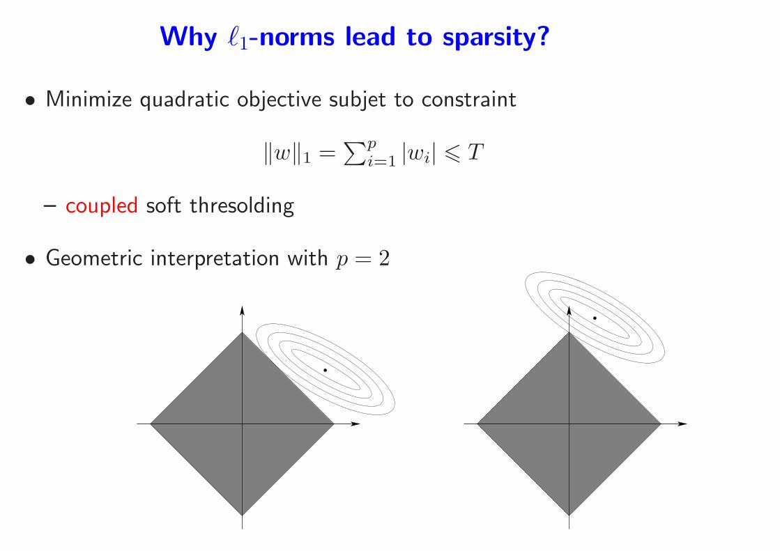
Why ℓ1-norms lead to sparsity?
• Minimize quadratic objective subjet to constraint
‖w‖1 =∑p
i=1 |wi| 6 T
– coupled soft thresolding
• Geometric interpretation with p = 2
ℓ1-norm regularization (linear setting)
• Data: covariates xi ∈ Rp, responses yi ∈ Y, i = 1, . . . , n
• Minimize with respect to loadings/weights w ∈ Rp:
n∑
i=1
ℓ(yi, w⊤xi) + λ‖w‖1
Error on data + Regularization
• Including a constant term b? Penalizing or constraining?
• Assumptions on loss:
– convex and differentiable in the second variable
– NB: with the square loss⇒ basis pursuit (signal processing) (Chen
et al., 2001), Lasso (statistics/machine learning) (Tibshirani, 1996)
Nonsmooth optimization
• Simple methods do not always work!
– Coordinate/steepest descent might not converge to a local
minimum
– Be careful!
• Optimization algorithms
– First order methods: good for large scale/low precision
– Second order methods: good for small scale/high precision
• Books: Boyd and Vandenberghe (2003), Bonnans et al. (2003),
Nocedal and Wright (2006), Borwein and Lewis (2000)
Algorithms for ℓ1-norms:
Gaussian hare vs. Laplacian tortoise
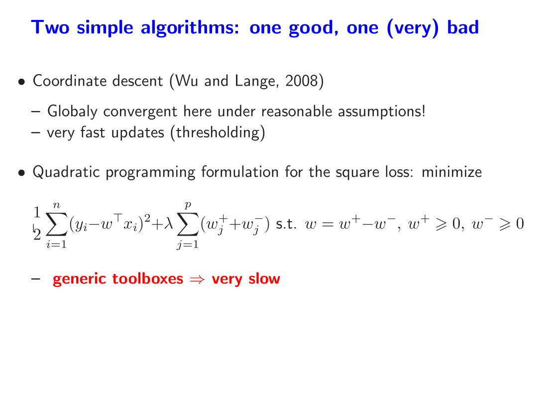
Two simple algorithms: one good, one (very) bad
• Coordinate descent (Wu and Lange, 2008)
– Globaly convergent here under reasonable assumptions!
– very fast updates (thresholding)
• Quadratic programming formulation for the square loss: minimize
1
2
n∑
i=1
(yi−w⊤xi)
2+λ
p∑
j=1
(w+j +w−
j ) s.t. w = w+−w−, w+> 0, w−
> 0
– generic toolboxes ⇒ very slow
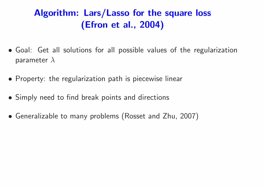
Algorithm: Lars/Lasso for the square loss
(Efron et al., 2004)
• Goal: Get all solutions for all possible values of the regularization
parameter λ
• Property: the regularization path is piecewise linear
• Simply need to find break points and directions
• Generalizable to many problems (Rosset and Zhu, 2007)

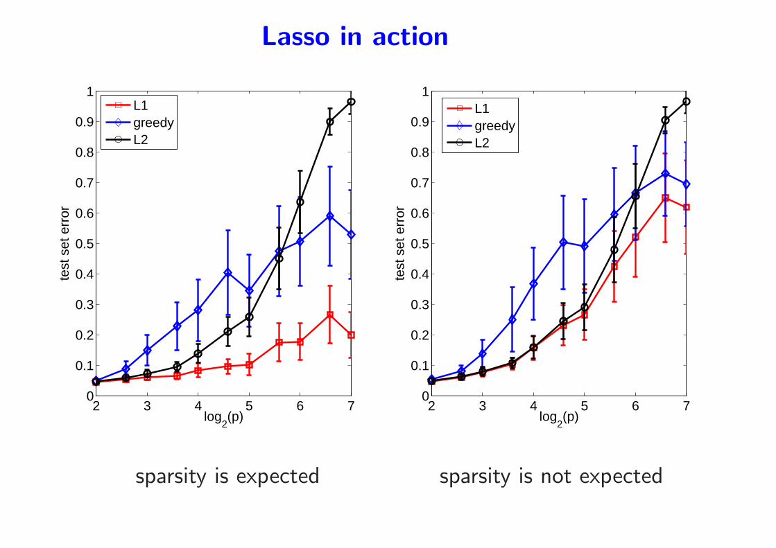
Lasso in action
• Piecewise linear paths
• When is it supposed to work?
– Simulations with random Gaussians, regularization parameter
estimated by cross-validation
– sparsity is expected or not
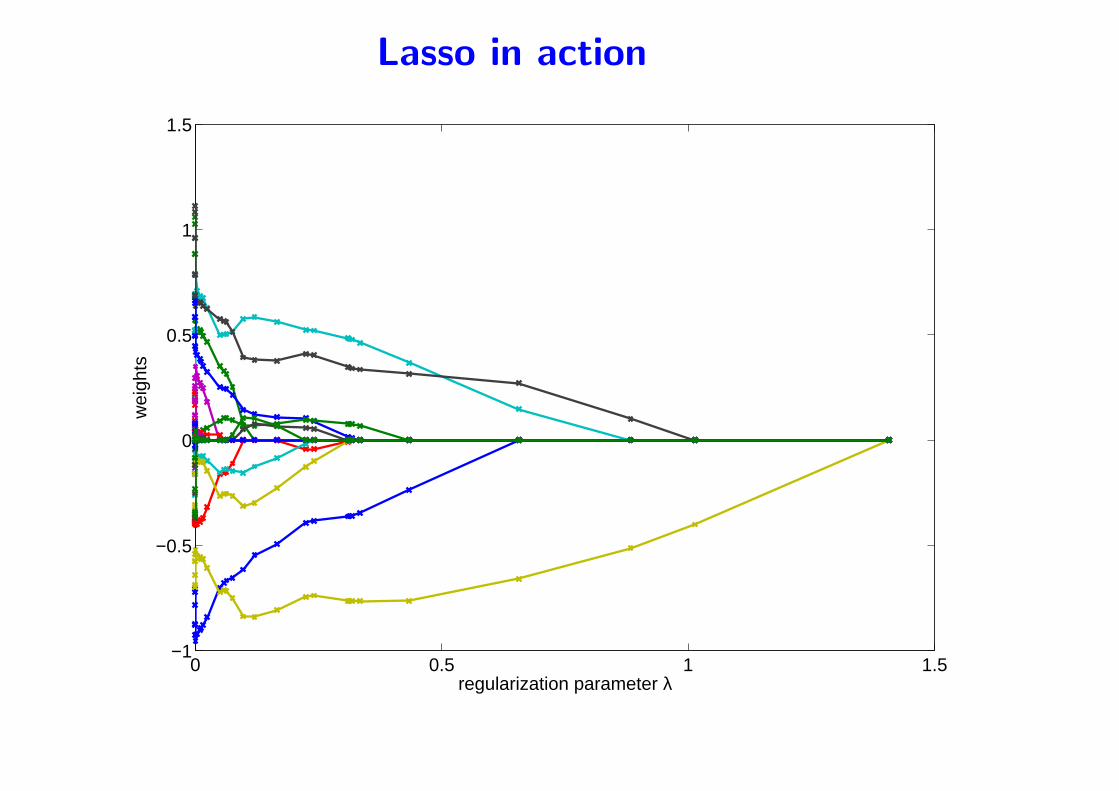
Lasso in action
0 0.5 1 1.5−1
−0.5
0
0.5
1
1.5
regularization parameter λ
wei
ghts
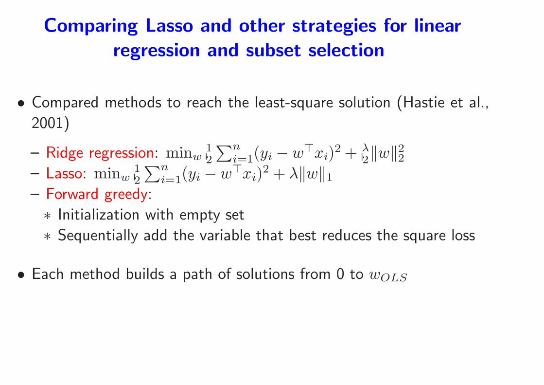
Comparing Lasso and other strategies for linear
regression and subset selection
• Compared methods to reach the least-square solution (Hastie et al.,
2001)
– Ridge regression: minw12
∑ni=1(yi − w
⊤xi)2 + λ
2‖w‖22
– Lasso: minw12
∑ni=1(yi − w
⊤xi)2 + λ‖w‖1
– Forward greedy:
∗ Initialization with empty set
∗ Sequentially add the variable that best reduces the square loss
• Each method builds a path of solutions from 0 to wOLS
Lasso in action
2 3 4 5 6 70
0.1
0.2
0.3
0.4
0.5
0.6
0.7
0.8
0.9
1
log2(p)
test
set
err
or
2 3 4 5 6 70
0.1
0.2
0.3
0.4
0.5
0.6
0.7
0.8
0.9
1
log2(p)
test
set
err
or
L1greedyL2
L1greedyL2
sparsity is expected sparsity is not expected

Part II - Outline
1. Losses for particular machine learning tasks
• Classification, regression, etc...
2. Regularization by Hilbert norms (kernel methods)
• Kernels and representer theorem
• Convex duality and optimization
• Kernel design
3. Regularization by sparsity-inducing norms
• ℓ1-norm regularization
• Multiple kernel learning
• Theoretical results
• Other extensions
Kernel learning with convex optimization
• Kernel methods work...
...with the good kernel!
⇒ Why not learn the kernel directly from data?
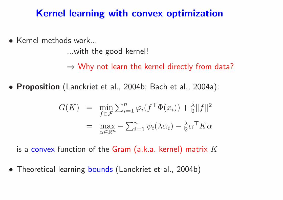
Kernel learning with convex optimization
• Kernel methods work...
...with the good kernel!
⇒ Why not learn the kernel directly from data?
• Proposition (Lanckriet et al., 2004b; Bach et al., 2004a):
G(K) = minf∈F
∑ni=1ϕi(f
⊤Φ(xi)) + λ2‖f‖
2
= maxα∈Rn
−∑n
i=1ψi(λαi)−λ2α
⊤Kα
is a convex function of the Gram (a.k.a. kernel) matrix K
• Theoretical learning bounds (Lanckriet et al., 2004b)
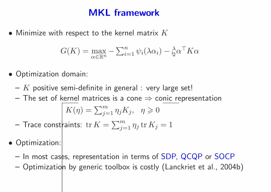
MKL framework
• Minimize with respect to the kernel matrix K
G(K) = maxα∈Rn
−∑n
i=1ψi(λαi)−λ2α
⊤Kα
• Optimization domain:
– K positive semi-definite in general : very large set!
– The set of kernel matrices is a cone ⇒ conic representation
K(η) =∑m
j=1 ηjKj, η > 0
– Trace constraints: trK =∑m
j=1 ηj trKj = 1
• Optimization:
– In most cases, representation in terms of SDP, QCQP or SOCP
– Optimization by generic toolbox is costly (Lanckriet et al., 2004b)
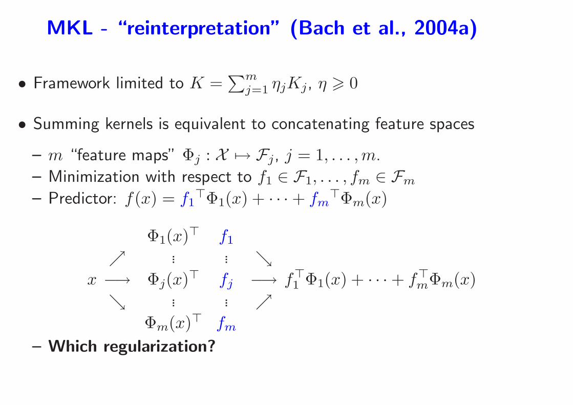
MKL - “reinterpretation” (Bach et al., 2004a)
• Framework limited to K =∑m
j=1 ηjKj, η > 0
• Summing kernels is equivalent to concatenating feature spaces
– m “feature maps” Φj : X 7→ Fj, j = 1, . . . ,m.
– Minimization with respect to f1 ∈ F1, . . . , fm ∈ Fm
– Predictor: f(x) = f1⊤Φ1(x) + · · ·+ fm
⊤Φm(x)
x
Φ1(x)⊤ f1
ր ... ... ց
−→ Φj(x)⊤ fj −→
ց ... ... ր
Φm(x)⊤ fm
f⊤1 Φ1(x) + · · ·+ f⊤mΦm(x)
– Which regularization?
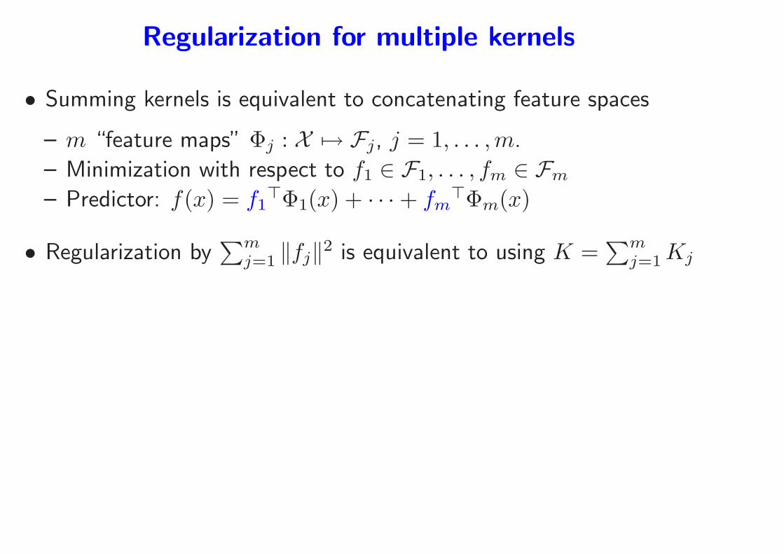
Regularization for multiple kernels
• Summing kernels is equivalent to concatenating feature spaces
– m “feature maps” Φj : X 7→ Fj, j = 1, . . . ,m.
– Minimization with respect to f1 ∈ F1, . . . , fm ∈ Fm
– Predictor: f(x) = f1⊤Φ1(x) + · · ·+ fm
⊤Φm(x)
• Regularization by∑m
j=1 ‖fj‖2 is equivalent to using K =
∑mj=1Kj
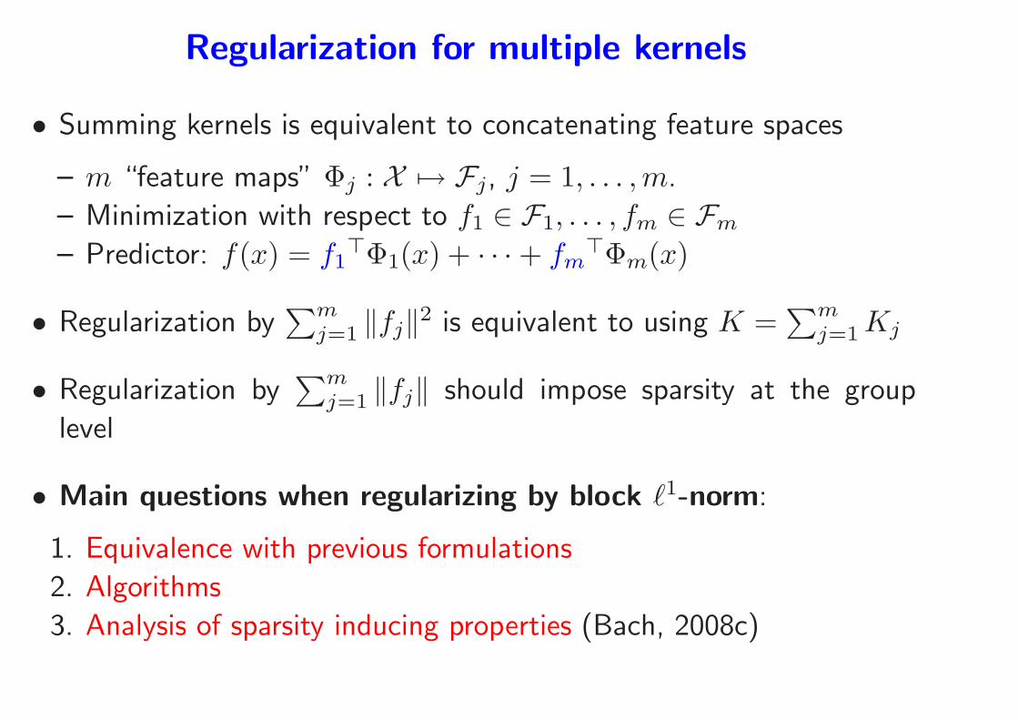
• Regularization by∑m
j=1 ‖fj‖ should impose sparsity at the group
level
• Main questions when regularizing by block ℓ1-norm:
1. Equivalence with previous formulations
2. Algorithms
3. Analysis of sparsity inducing properties (Bach, 2008c)
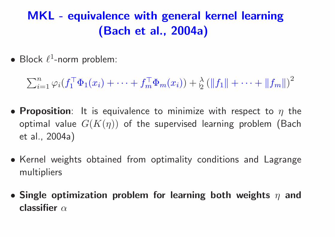
MKL - equivalence with general kernel learning
(Bach et al., 2004a)
• Block ℓ1-norm problem:
∑ni=1ϕi(f
⊤1 Φ1(xi) + · · ·+ f⊤mΦm(xi)) + λ
2 (‖f1‖+ · · ·+ ‖fm‖)2
• Proposition: It is equivalence to minimize with respect to η the
optimal value G(K(η)) of the supervised learning problem (Bach
et al., 2004a)
• Kernel weights obtained from optimality conditions and Lagrange
multipliers
• Single optimization problem for learning both weights η and
classifier α
Algorithms for MKL
• (very) costly optimization with SDP, QCQP ou SOCP
– n > 1, 000− 10, 000, m > 100 not possible
– “loose” required precision ⇒ first order methods
• Dual coordinate ascent (SMO) with smoothing (Bach et al., 2004a)
• Optimization of G(K) by cutting planes (Sonnenburg et al., 2006)
• Optimization of G(K) with steepest descent with smoothing
(Rakotomamonjy et al., 2008)
• Regularization path (Bach et al., 2004b)
Applications
• Several applications
– Bioinformatics (Lanckriet et al., 2004a)
– Speech processing (Longworth and Gales, 2008)
– Image annotation (Harchaoui and Bach, 2007; Varma and Ray,
2007; Bosch et al., 2008)
• Two potential uses
– Fusion of heterogeneous data sources
– Learning hyperparameters
– Sparsity in non-linear settings
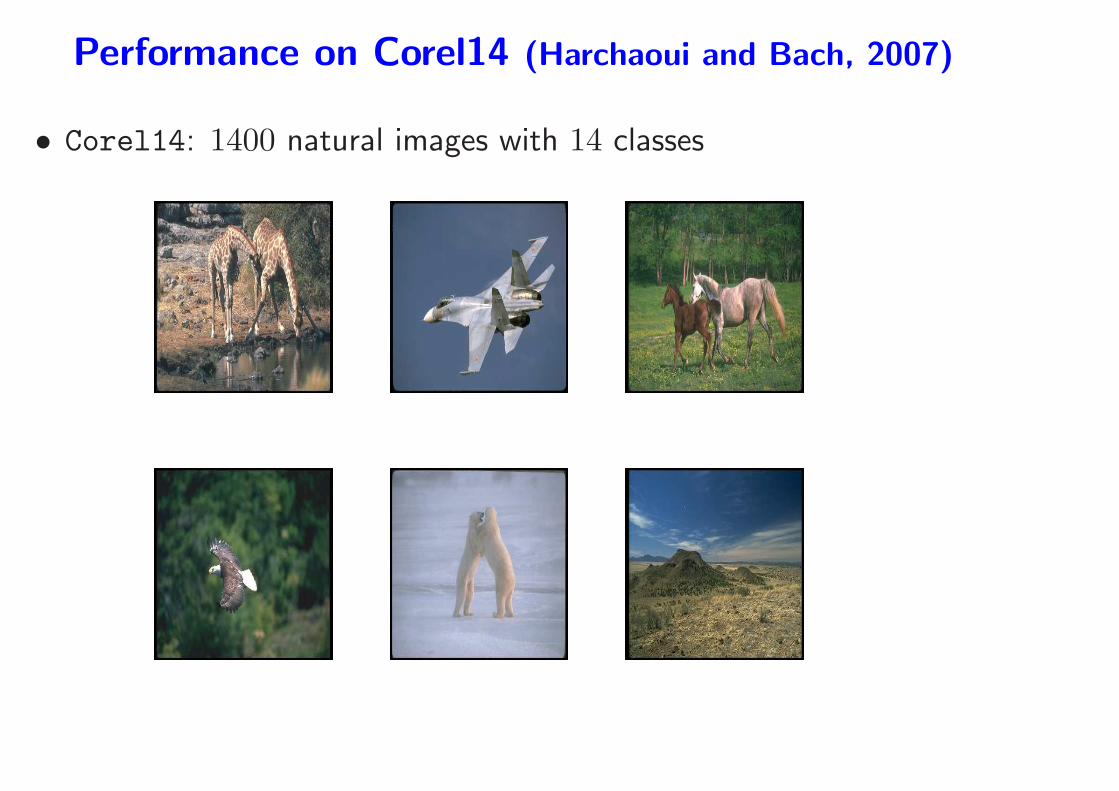
Performance on Corel14 (Harchaoui and Bach, 2007)
• Corel14: 1400 natural images with 14 classes
Performance on Corel14 (Harchaoui and Bach, 2007)
Error rates
• Histogram kernels (H)
• Walk kernels (W)
• Tree-walk kernels (TW)
• Weighted tree-walks(wTW)
• MKL (M) H W TW wTW M
0.05
0.06
0.07
0.08
0.09
0.1
0.11
0.12
Tes
t err
or
Kernels
Performance comparison on Corel14
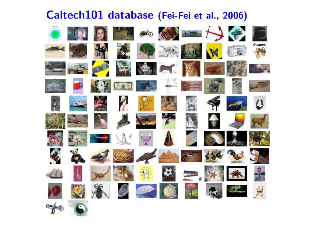
Caltech101 database (Fei-Fei et al., 2006)
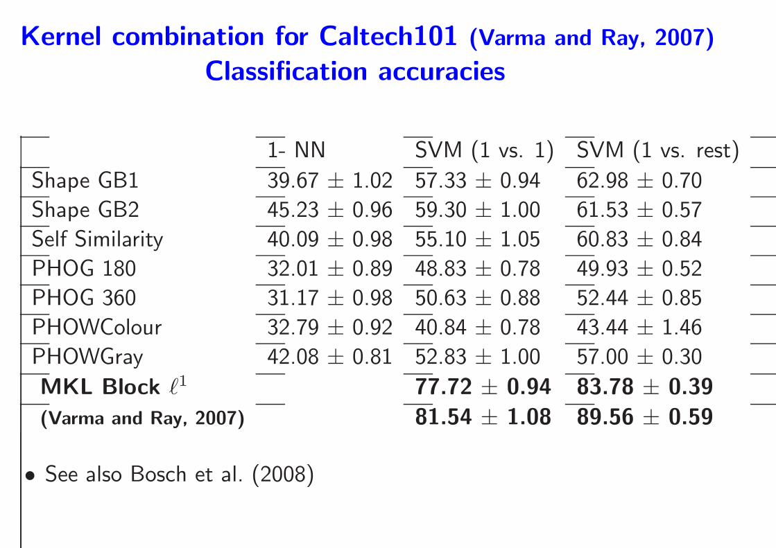
Kernel combination for Caltech101 (Varma and Ray, 2007)
Classification accuracies
1- NN SVM (1 vs. 1) SVM (1 vs. rest)
Shape GB1 39.67 ± 1.02 57.33 ± 0.94 62.98 ± 0.70
Shape GB2 45.23 ± 0.96 59.30 ± 1.00 61.53 ± 0.57
Self Similarity 40.09 ± 0.98 55.10 ± 1.05 60.83 ± 0.84
PHOG 180 32.01 ± 0.89 48.83 ± 0.78 49.93 ± 0.52
PHOG 360 31.17 ± 0.98 50.63 ± 0.88 52.44 ± 0.85
PHOWColour 32.79 ± 0.92 40.84 ± 0.78 43.44 ± 1.46
PHOWGray 42.08 ± 0.81 52.83 ± 1.00 57.00 ± 0.30
MKL Block ℓ1 77.72 ± 0.94 83.78 ± 0.39
(Varma and Ray, 2007) 81.54 ± 1.08 89.56 ± 0.59
• See also Bosch et al. (2008)

Part II - Outline
1. Losses for particular machine learning tasks
• Classification, regression, etc...
2. Regularization by Hilbert norms (kernel methods)
• Kernels and representer theorem
• Convex duality and optimization
• Kernel design
3. Regularization by sparsity-inducing norms
• ℓ1-norm regularization
• Multiple kernel learning
• Theoretical results
• Other extensions

Learning on matrices
• Example 1: matrix completion
– Given a matrix M ∈ Rn×p and a subset of observed entries,
estimate all entries
– Many applications: graph learning, collaborative filtering (Breese
et al., 1998; Heckerman et al., 2000; Salakhutdinov et al., 2007)
• Example 2: multi-task learning (Obozinski et al., 2007; Pontil et al., 2007)
– Common features for m learning problems ⇒ m different weights,
i.e., W = (w1, . . . , wm) ∈ Rp×m
– Numerous applications
• Example 3: image denoising (Elad and Aharon, 2006; Mairal et al., 2008)
– Simultaneously denoise all patches of a given image
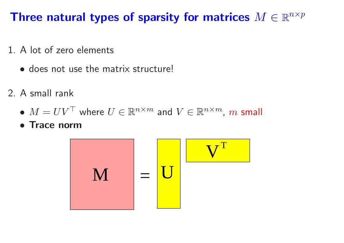
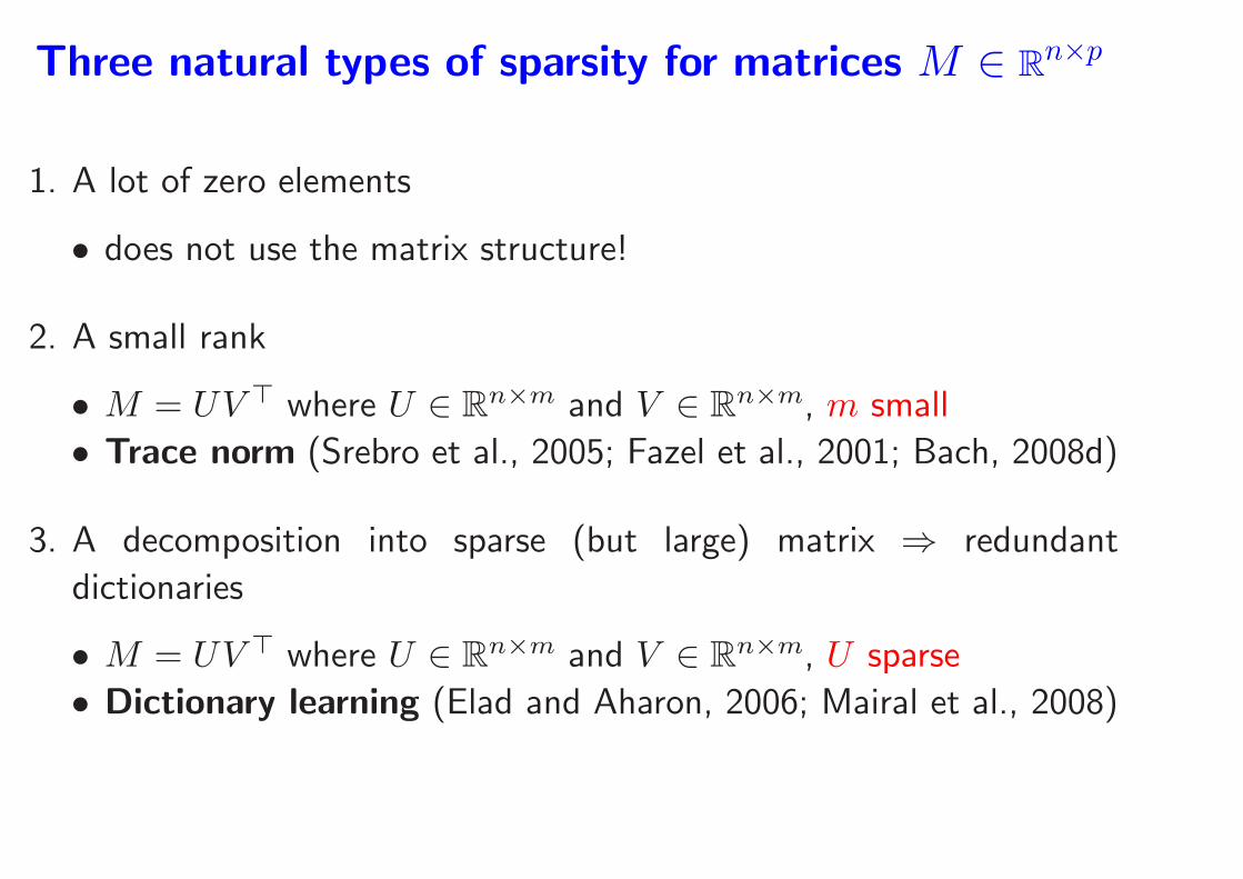
Three natural types of sparsity for matrices M ∈ Rn×p
1. A lot of zero elements
• does not use the matrix structure!
2. A small rank
• M = UV ⊤ where U ∈ Rn×m and V ∈ R
n×m, m small
• Trace norm
U=V
M
T
Three natural types of sparsity for matrices M ∈ Rn×p
1. A lot of zero elements
• does not use the matrix structure!
2. A small rank
• M = UV ⊤ where U ∈ Rn×m and V ∈ R
n×m, m small
• Trace norm (Srebro et al., 2005; Fazel et al., 2001; Bach, 2008d)
3. A decomposition into sparse (but large) matrix ⇒ redundant
dictionaries
• M = UV ⊤ where U ∈ Rn×m and V ∈ R
n×m, U sparse
• Dictionary learning (Elad and Aharon, 2006; Mairal et al., 2008)
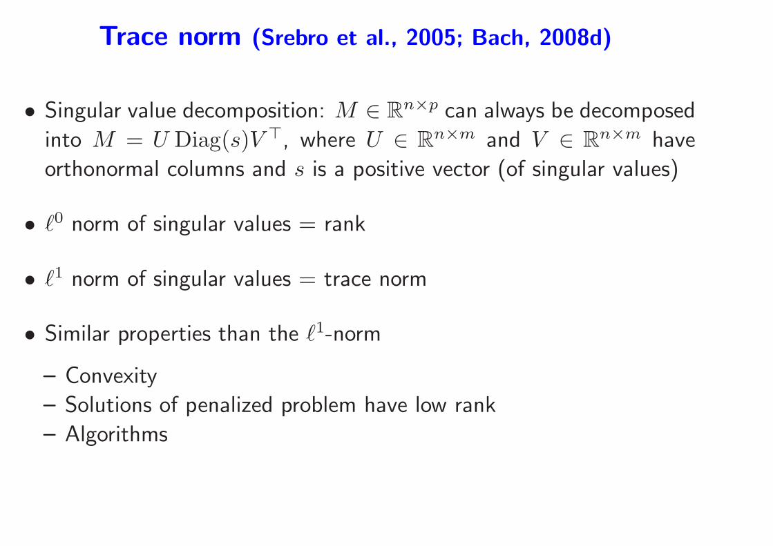
Trace norm (Srebro et al., 2005; Bach, 2008d)
• Singular value decomposition: M ∈ Rn×p can always be decomposed
into M = U Diag(s)V ⊤, where U ∈ Rn×m and V ∈ R
n×m have
orthonormal columns and s is a positive vector (of singular values)
• ℓ0 norm of singular values = rank
• ℓ1 norm of singular values = trace norm
• Similar properties than the ℓ1-norm
– Convexity
– Solutions of penalized problem have low rank
– Algorithms
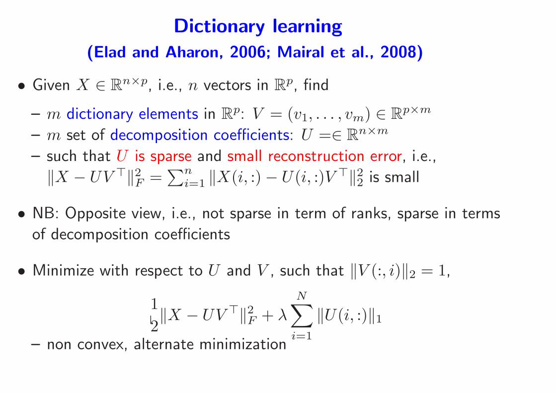
Dictionary learning
(Elad and Aharon, 2006; Mairal et al., 2008)
• Given X ∈ Rn×p, i.e., n vectors in R
p, find
– m dictionary elements in Rp: V = (v1, . . . , vm) ∈ R
p×m
– m set of decomposition coefficients: U =∈ Rn×m
– such that U is sparse and small reconstruction error, i.e.,
‖X − UV ⊤‖2F =∑n
i=1 ‖X(i, :)− U(i, :)V ⊤‖22 is small
• NB: Opposite view, i.e., not sparse in term of ranks, sparse in terms
of decomposition coefficients
• Minimize with respect to U and V , such that ‖V (:, i)‖2 = 1,
1
2‖X − UV ⊤‖2F + λ
N∑
i=1
‖U(i, :)‖1
– non convex, alternate minimization
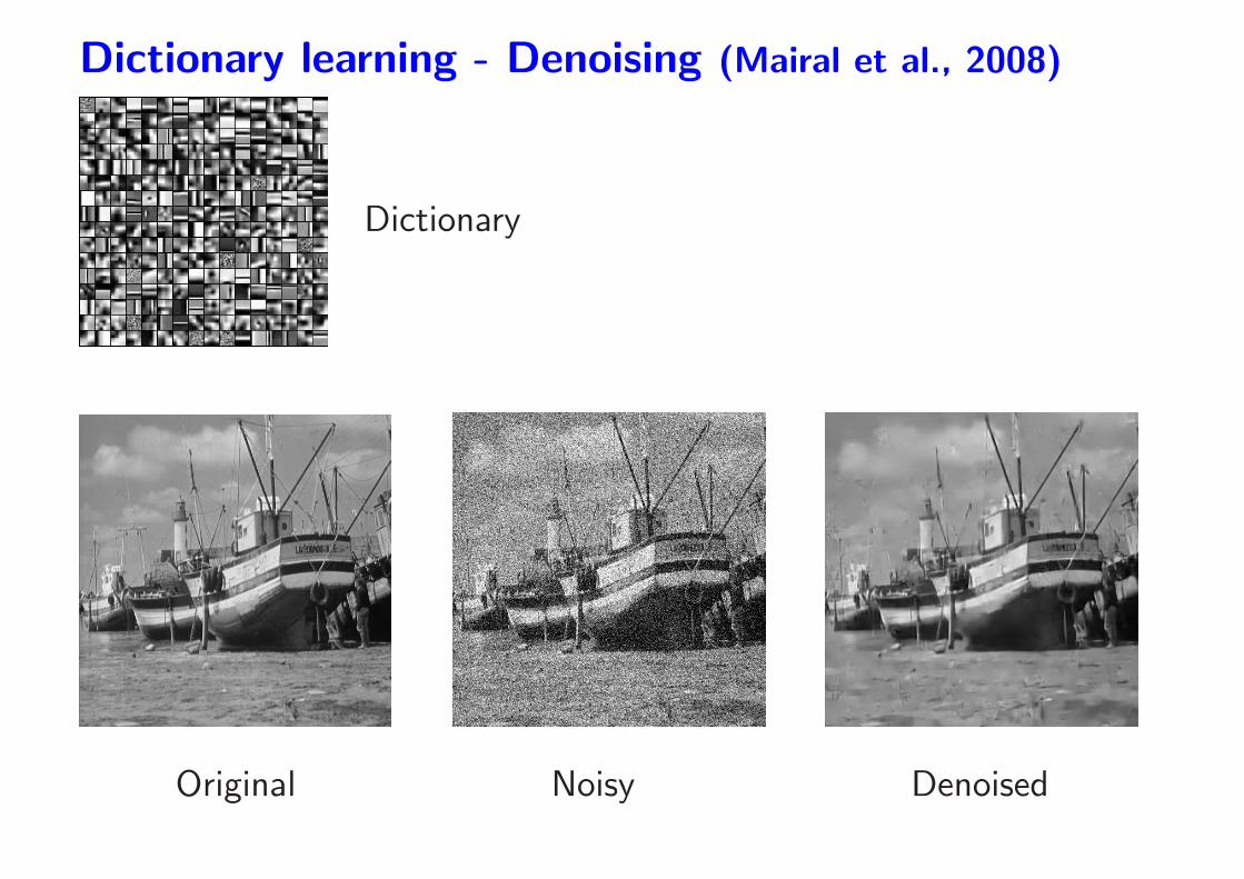
Dictionary learning - Denoising (Mairal et al., 2008)
Dictionary
Original Noisy Denoised
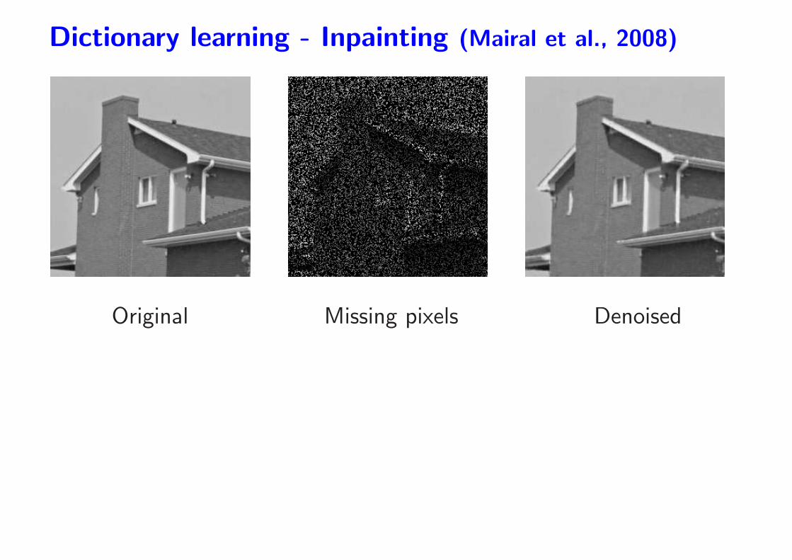
Dictionary learning - Inpainting (Mairal et al., 2008)
Original Missing pixels Denoised
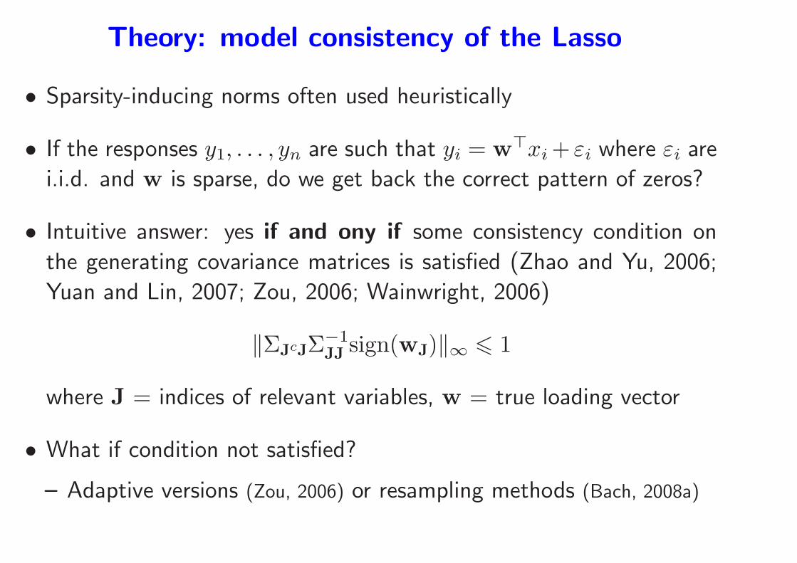
Theory: model consistency of the Lasso
• Sparsity-inducing norms often used heuristically
• If the responses y1, . . . , yn are such that yi = w⊤xi + εi where εi are
i.i.d. and w is sparse, do we get back the correct pattern of zeros?
• Intuitive answer: yes if and ony if some consistency condition on
the generating covariance matrices is satisfied (Zhao and Yu, 2006;
Yuan and Lin, 2007; Zou, 2006; Wainwright, 2006)
‖ΣJcJΣ−1JJ
sign(wJ)‖∞ 6 1
where J = indices of relevant variables, w = true loading vector
• What if condition not satisfied?
– Adaptive versions (Zou, 2006) or resampling methods (Bach, 2008a)
High-dimensional setting
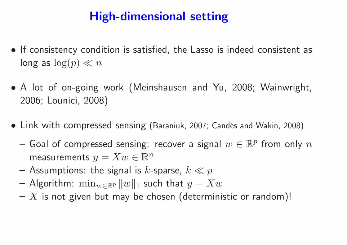
• If consistency condition is satisfied, the Lasso is indeed consistent as
long as log(p)≪ n
• A lot of on-going work (Meinshausen and Yu, 2008; Wainwright,
2006; Lounici, 2008)
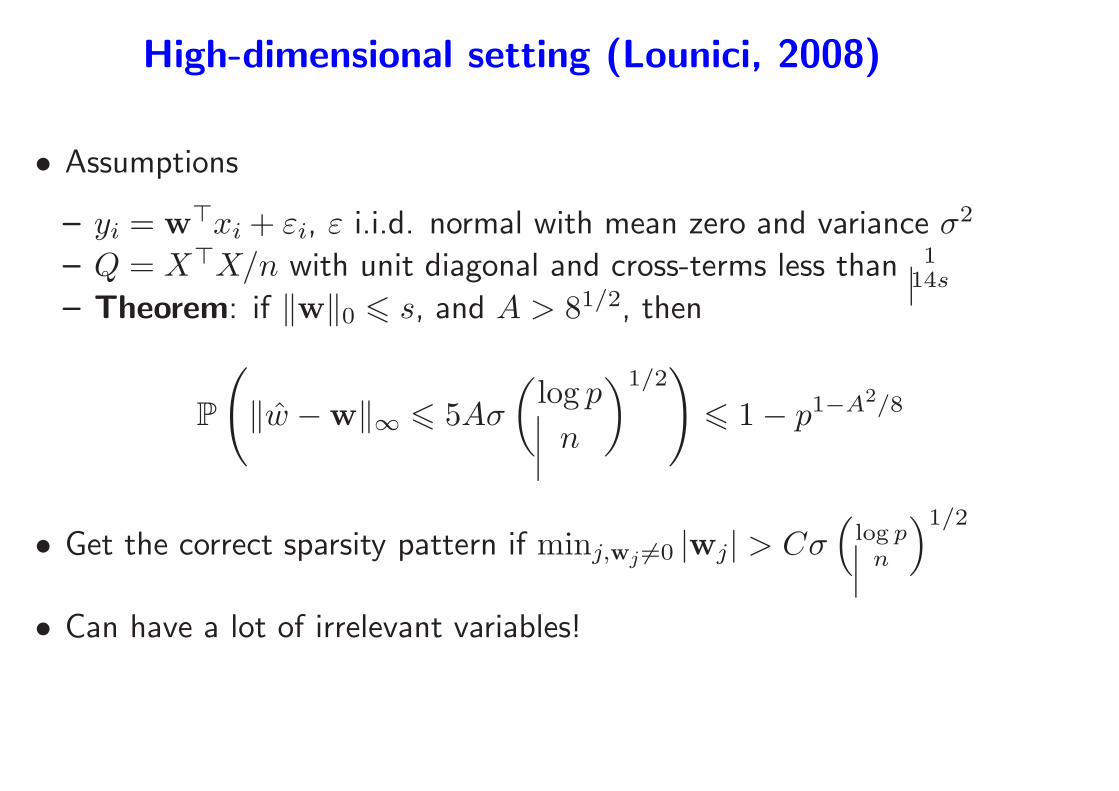
High-dimensional setting (Lounici, 2008)
• Assumptions
– yi = w⊤xi + εi, ε i.i.d. normal with mean zero and variance σ2
– Q = X⊤X/n with unit diagonal and cross-terms less than 114s
– Theorem: if ‖w‖0 6 s, and A > 81/2, then
P
(
‖w −w‖∞ 6 5Aσ
(
log p
n
)1/2)
6 1− p1−A2/8
• Get the correct sparsity pattern if minj,wj 6=0 |wj| > Cσ(
log pn
)1/2
• Can have a lot of irrelevant variables!
High-dimensional setting
• If consistency condition is satisfied, the Lasso is indeed consistent as
long as log(p)≪ n
• A lot of on-going work (Meinshausen and Yu, 2008; Wainwright,
2006; Lounici, 2008)
• Link with compressed sensing (Baraniuk, 2007; Candes and Wakin, 2008)
– Goal of compressed sensing: recover a signal w ∈ Rp from only n
measurements y = Xw ∈ Rn
– Assumptions: the signal is k-sparse, k ≪ p
– Algorithm: minw∈Rp ‖w‖1 such that y = Xw
– X is not given but may be chosen (deterministic or random)!
Summary - sparsity-inducing norms
• Sparsity through non Euclidean norms
• Alternative approaches to sparsity
– greedy approaches - Bayesian approaches
• Important (often non treated) question: when does sparsity actually
help?
• Current research directions
– Algorithms, algorithms, algorithms!
– Structured norm for structured situations (variables are usually not
created equal) ⇒ hierarchical Lasso or MKL (Zhao et al., 2008;
Bach, 2008b)
Conclusion - Course Outline
1. Theory
• Probabilistic model and universal consistency
• Local averaging methods
• Empirical risk minimization
2. Algorithms
• Losses for particular machine learning tasks
• Regularization by Hilbert norms (kernel methods)
– Algorithms
– Kernel design
• Regularization by sparsity-inducing norms
– ℓ1-norm regularization
– Multiple kernel learning
References
N. Aronszajn. Theory of reproducing kernels. Trans. Am. Math. Soc., 68:337–404, 1950.
F. Bach. Bolasso: model consistent lasso estimation through the bootstrap. In Proceedings of the
Twenty-fifth International Conference on Machine Learning (ICML), 2008a.
F. Bach. Exploring large feature spaces with hierarchical multiple kernel learning. In Adv. NIPS, 2008b.
F. R. Bach. Consistency of the group Lasso and multiple kernel learning. Journal of Machine Learning
Research, pages 1179–1225, 2008c.
F. R. Bach. Consistency of trace norm minimization. Journal of Machine Learning Research, to appear,
2008d.
F. R. Bach and M. I. Jordan. Kernel independent component analysis. Journal of Machine Learning
Research, 3:1–48, 2002.
F. R. Bach, G. R. G. Lanckriet, and M. I. Jordan. Multiple kernel learning, conic duality, and the SMO
algorithm. In Proceedings of the International Conference on Machine Learning (ICML), 2004a.
F. R. Bach, R. Thibaux, and M. I. Jordan. Computing regularization paths for learning multiple kernels.
In Advances in Neural Information Processing Systems 17, 2004b.
F. R. Bach, D. Heckerman, and E. Horvitz. Considering cost asymmetry in learning classifiers. Journal
of Machine Learning Research, 7:1713–1741, 2006.
Richard Baraniuk. Compressive sensing. IEEE Signal Processing Magazine, 24(4):118–121, 2007.
J. F. Bonnans, J. C. Gilbert, C. Lemarechal, and C. A. Sagastizbal. Numerical Optimization Theoretical
and Practical Aspects. Springer, 2003.
Karsten M. Borgwardt, Cheng Soon Ong, Stefan Schonauer, S. V. N. Vishwanathan, Alex J. Smola,
and Hans-Peter Kriegel. Protein function prediction via graph kernels. Bioinformatics, 21, 2005.
J. M. Borwein and A. S. Lewis. Convex Analysis and Nonlinear Optimization. Number 3 in CMS
Books in Mathematics. Springer-Verlag, 2000.
A. Bosch, Zisserman A., and X. Munoz. Image classification using rois and multiple kernel learning.
International Journal of Computer Vision, 2008. submitted.
L. Bottou and C. J. Lin. Support vector machine solvers. In Large scale kernel machines, 2007.
Leon Bottou and Olivier Bousquet. Learning using large datasets. In Mining Massive DataSets for
Security, NATO ASI Workshop Series. IOS Press, Amsterdam, 2008. URL http://leon.bottou.
org/papers/bottou-bousquet-2008b. to appear.
S. Boyd and L. Vandenberghe. Convex Optimization. Cambridge Univ. Press, 2003.
J. S. Breese, D. Heckerman, and C. Kadie. Empirical analysis of predictive algorithms for collaborative
filtering. In 14th Conference on Uncertainty in Artificial Intelligence, pages 43–52, Madison, W.I.,
1998. Morgan Kaufman.
Emmanuel Candes and Michael Wakin. An introduction to compressive sampling. IEEE Signal
Processing Magazine, 25(2):21–30, 2008.
O. Chapelle. Training a support vector machine in the primal. Neural Computation, 19(5):1155–1178,
2007.
Scott Shaobing Chen, David L. Donoho, and Michael A. Saunders. Atomic decomposition by basis
pursuit. SIAM Rev., 43(1):129–159, 2001. ISSN 0036-1445.
B. Efron, T. Hastie, I. Johnstone, and R. Tibshirani. Least angle regression. Ann. Stat., 32:407, 2004.
M. Elad and M. Aharon. Image denoising via sparse and redundant representations over learned
dictionaries. IEEE Trans. Image Proc., 15(12):3736–3745, 2006.
M. Fazel, H. Hindi, and S. P. Boyd. A rank minimization heuristic with application to minimum order
system approximation. In Proceedings American Control Conference, volume 6, pages 4734–4739,
2001.
L. Fei-Fei, R. Fergus, and P. Perona. Learning generative visual models for 101 object categories.
Computer Vision and Image Understanding, 2006.
S. Fine and K. Scheinberg. Efficient SVM training using low-rank kernel representations. Journal of
Machine Learning Research, 2:243–264, 2001.
P. A. Flach. The geometry of ROC space: understanding machine learning metrics through ROC
isometrics. In International Conference on Machine Learning (ICML), 2003.
Thomas Gartner, Peter A. Flach, and Stefan Wrobel. On graph kernels: Hardness results and efficient
alternatives. In COLT, 2003.
K. Grauman and T. Darrell. The pyramid match kernel: Efficient learning with sets of features. J.
Mach. Learn. Res., 8:725–760, 2007. ISSN 1533-7928.
Z. Harchaoui and F. R. Bach. Image classification with segmentation graph kernels. In Proceedings of
the Conference on Computer Vision and Pattern Recognition (CVPR), 2007.
T. Hastie, R. Tibshirani, and J. Friedman. The Elements of Statistical Learning. Springer-Verlag,
2001.
T. Hastie, S. Rosset, R. Tibshirani, and J. Zhu. The entire regularization path for the support vector
machine. Journal of Machine Learning Research, 5:1391–1415, 2005.
David Haussler. Convolution kernels on discrete structures. Technical report, UCSC, 1999.
D. Heckerman, D. M. Chickering, C. Meek, R. Rounthwaite, and C. Kadie. Dependency networks for
inference, collaborative filtering, and data visualization. J. Mach. Learn. Res., 1:49–75, 2000.
M. Hein and O. Bousquet. Hilbertian metrics and positive-definite kernels on probability measures. In
AISTATS, 2004.
R. Herbrich, T. Graepel, and K. Obermayer. Large margin rank boundaries for ordinal regression. In
Advances in Large Margin Classifiers. MIT Press, Cambridge, MA, 2000.
T. Joachims. Optimizing search engines using clickthrough data. In ACM SIGKDD Conference on
Knowledge Discovery and Data Mining (KDD), pages 133–142, 2002.
T. Joachims. Making large-scale support vector machine learning practical. In Advances in kernel
methods — Support Vector learning. MIT Press, 1998.
Hisashi Kashima, Koji Tsuda, and Akihiro Inokuchi. Kernels for graphs. In Kernel Methods in
Computational Biology. MIT Press, 2004.
G. S. Kimeldorf and G. Wahba. Some results on Tchebycheffian spline functions. J. Math. Anal.
Applicat., 33:82–95, 1971.
G. R. G. Lanckriet, T. De Bie, N. Cristianini, M. I. Jordan, and W. S. Noble. A statistical framework
for genomic data fusion. Bioinf., 20:2626–2635, 2004a.
G. R. G. Lanckriet, N. Cristianini, L. El Ghaoui, P. Bartlett, and M. I. Jordan. Learning the kernel
matrix with semidefinite programming. Journal of Machine Learning Research, 5:27–72, 2004b.
S. Lazebnik, C. Schmid, and J. Ponce. Beyond bags of features: Spatial pyramid matching for
recognizing natural scene categories. In Proc. CVPR, 2006.
C. Longworth and M. J. F. Gales. Multiple kernel learning for speaker verification. In Proceedings of
the IEEE International Conference on Acoustics, Speech and Signal Processing (ICASSP), 2008.
G. Loosli, S. Canu, S. Vishwanathan, A. Smola, and M. Chattopadhyay. Boıte a outils SVM simple et
rapide. Revue dIntelligence Artificielle, 19(4-5):741–767, 2005.
K. Lounici. Sup-norm convergence rate and sign concentration property of Lasso and Dantzig
estimators. Electronic Journal of Statistics, 2, 2008.
J. Mairal, G. Sapiro, and M. Elad. Learning multiscale sparse representations for image and video
restoration. SIAM Multiscale Modeling and Simulation, 7(1):214–241, 2008.
N. Meinshausen and B. Yu. Lasso-type recovery of sparse representations for high-dimensional data.
Ann. Stat., page to appear, 2008.
F. Meyer. Hierarchies of partitions and morphological segmentation. In Scale-Space and Morphology
in Computer Vision. Springer-Verlag, 2001.
Jorge Nocedal and Stephen J. Wright. Numerical Optimization, chapter 1. Springer, 2nd edition, 2006.
G. Obozinski, B. Taskar, and M. I. Jordan. Multi-task feature selection. Technical report, UC Berkeley,
2007.
J. Platt. Fast training of support vector machines using sequential minimal optimization. In Advances
in Kernel Methods: Support Vector Learning, 1998.
M. Pontil, A. Argyriou, and T. Evgeniou. Multi-task feature learning. In Advances in Neural Information
Processing Systems, 2007.
A. Rakotomamonjy, F. R. Bach, S. Canu, and Y. Grandvalet. Simplemkl. Journal of Machine Learning
Research, to appear, 2008.
Jan Ramon and Thomas Gartner. Expressivity versus efficiency of graph kernels. In First International
Workshop on Mining Graphs, Trees and Sequences, 2003.
S. Rosset and J. Zhu. Piecewise linear regularized solution paths. Ann. Statist., 35(3):1012–1030,
2007.
R. Salakhutdinov, A. Mnih, and G. Hinton. Restricted boltzmann machines for collaborative filtering.
In ICML ’07: Proceedings of the 24th international conference on Machine learning, pages 791–798,
New York, NY, USA, 2007. ACM.
B. Scholkopf and A. J. Smola. Learning with Kernels. MIT Press, 2001.
B. Scholkopf, J. C. Platt, J. S. Shawe-Taylor, A. J. Smola, and R. C. Williamson. Estimating the
support of a high-dimensional distribution. Neural Computation, 13(7):1443–1471, 2001.
S. Shalev-Shwartz, Y. Singer, and N. Srebro. Pegasos: Primal estimated sub-gradient solver for SVM.
In Proceedings of the International Conference on Machine Learning (ICML), 2007.
J. Shawe-Taylor and N. Cristianini. Kernel Methods for Pattern Analysis. Camb. U. P., 2004.
S. Sonnenburg, G. Rasch, C. Schafer, and B. Scholkopf. Large scale multiple kernel learning. Journal
of Machine Learning Research, 7:1531–1565, 2006.
N. Srebro, J. D. M. Rennie, and T. S. Jaakkola. Maximum-margin matrix factorization. In Advances
in Neural Information Processing Systems 17, 2005.
B. Taskar. Structured prediction: A large margin approach. In NIPS Tutorial, 2005. URL media.
nips.cc/Conferences/2007/Tutorials/Slides/taskar-NIPS-07-tutorial.ppt.
R. Tibshirani. Regression shrinkage and selection via the lasso. Journal of The Royal Statistical Society
Series B, 58(1):267–288, 1996.
M. Varma and D. Ray. Learning the discriminative power-invariance trade-off. In Proc. ICCV, 2007.
R. Vert and J.-P. Vert. Consistency and convergence rates of one-class svms and related algorithms.
Journal of Machine Learning Research, 7:817–854, 2006.
S. V. N. Vishwanathan, A. J. Smola, and M. Murty. Simplesvm. In Proceedings of the International
Conference on Machine Learning (ICML), 2003.
G. Wahba. Spline Models for Observational Data. SIAM, 1990.
M. J. Wainwright. Sharp thresholds for noisy and high-dimensional recovery of sparsity using ℓ1-
constrained quadratic programming. Technical Report 709, Dpt. of Statistics, UC Berkeley, 2006.
C. Watkins. Dynamic alignment kernels. Technical report, RHUL, 1999.
Tong Tong Wu and Kenneth Lange. Coordinate descent algorithms for lasso penalized regression. Ann.
Appl. Stat., 2(1):224–244, 2008.
M. Yuan and Y. Lin. On the non-negative garrotte estimator. Journal of The Royal Statistical Society
Series B, 69(2):143–161, 2007.
P. Zhao and B. Yu. On model selection consistency of Lasso. Journal of Machine Learning Research,
7:2541–2563, 2006.
P. Zhao, G. Rocha, and B. Yu. Grouped and hierarchical model selection through composite absolute
penalties. Annals of Statistics, To appear, 2008.
H. Zou. The adaptive Lasso and its oracle properties. Journal of the American Statistical Association,
101:1418–1429, December 2006.
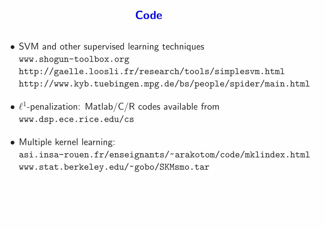
Code
• SVM and other supervised learning techniques
www.shogun-toolbox.org
http://gaelle.loosli.fr/research/tools/simplesvm.html
http://www.kyb.tuebingen.mpg.de/bs/people/spider/main.html
• ℓ1-penalization: Matlab/C/R codes available from
www.dsp.ece.rice.edu/cs
• Multiple kernel learning:
asi.insa-rouen.fr/enseignants/~arakotom/code/mklindex.html
www.stat.berkeley.edu/~gobo/SKMsmo.tar
Conclusion - Interesting problems
• Kernel design for computer vision
– Benefits of “kernelizing” existing representations
– Combining kernels
• Sparsity and computer vision
– Going beyond image denoising
• Large numbers of classes
– Theoretical and algorithmic challenges
• Structured output