STRUCTURED PSEUDOSPECTRA AND THE - TU Berlin

SIAM J. MATRIX ANAL. APPL. c© 2010 Society for Industrial and Applied MathematicsVol. 31, No. 5, pp. 2860–2881

STRUCTURED PSEUDOSPECTRA AND THE CONDITION OF ANONDEROGATORY EIGENVALUE∗

MICHAEL KAROW†

Abstract. Let λ be a nonderogatory eigenvalue of A ∈ Cn×n of algebraic multiplicity m. Thesensitivity of λ with respect to matrix perturbations of the form A � A + Δ, Δ ∈ Δ, is measuredby the structured condition number κΔ(A,λ). Here Δ denotes the set of admissible perturbations.However, if Δ is not a vector space over C, then κΔ(A,λ) provides only incomplete informationabout the mobility of λ under small perturbations from Δ. The full information is then given bythe set KΔ(x, y) = {y∗Δx; Δ ∈ Δ, ‖Δ‖ ≤ 1} ⊂ C that depends on Δ, a pair of normalized rightand left eigenvectors x, y, and the norm ‖ · ‖ that measures the size of the perturbations. We alwayshave κΔ(A, λ) = max{|z|1/m; z ∈ KΔ(x, y)}. Furthermore, KΔ(x, y) determines the shape andgrowth of the Δ-structured pseudospectrum in a neighborhood of λ. In this paper we study thesets KΔ(x, y) and obtain methods for computing them. In doing so we obtain explicit formulae forstructured eigenvalue condition numbers with respect to many important perturbation classes.

Key words. eigenvalues, structured perturbations, pseudospectra, condition numbers

AMS subject classifications. 15A18, 15A57, 65F15, 65F35

DOI. 10.1137/070695836

Notation. The symbols R and C denote the sets of real and complex numbers,respectively. Km×n is the set of m× n matrices and Kn = Kn×1 is the set of columnvectors of length n, K ∈ {R,C}. By A�, A, A∗, �A, �A, and tr(A) we denote thetranspose, the conjugate, the conjugate transpose, the real and the imaginary parts,and the trace of A ∈ Cm×n. Furthermore, In stands for the n×n unit matrix. Finally,n = {1, . . . , n} for any positive integer n.

1. Introduction. The subject of this paper are the sets

KΔ(x, y) = { y∗Δx; Δ ∈ Δ, ‖Δ‖ ≤ 1 }, x, y ∈ Cn×n,(1.1)

where ‖·‖ is a norm on Cn×n and Δ ⊆ Cn×n is assumed to be a closed cone (the lattermeans that Δ ∈ Δ implies rΔ ∈ Δ for all r ≥ 0). Our motivation for consideringthese sets stems from eigenvalue perturbation analysis by means of pseudospectra.The sets KΔ(x, y) provide the full first order information about the sensitivity of anonderogatory eigenvalue with respect to structured matrix perturbations. This isexplained in some detail in the following discussion.

Let λ ∈ C be a nonderogatory eigenvalue of algebraic multiplicity m of A ∈ Cn×n.Let x ∈ Cn \ {0} be a right eigenvector, i.e., Ax = λx. Then there exists a uniqueleft generalized eigenvector y ∈ Cn \ 0 satisfying

y∗(A− λ In)m = 0, y∗(A− λ In)

m−1 = 0, y∗x = 1.

Let y∗ = y∗(A−λ In)m−1, and let ‖ · ‖ be an arbitrary norm on Cn×n. Under a small

perturbation of A of the form

A� A(Δ) = A+Δ, Δ ∈ Cn×n,(1.2)

∗Received by the editors June 29, 2007; accepted for publication (in revised form) by M. EmbreeAugust 3, 2010; published electronically November 30, 2010.

http://www.siam.org/journals/simax/31-5/69583.html†Matheon, Technische Universitat Berlin, D-10623 Berlin, Germany ([email protected]).

2860

STRUCTURED PSEUDOSPECTRA AND THE CONDITION 2861

the eigenvalue λ splits into m eigenvalues λ1(Δ), . . . , λm(Δ) of A(Δ) with the firstorder expansion [16]

λj(Δ) = λ+ θj(Δ) +O(‖Δ‖2/m), j ∈ m,(1.3)

where θ1(Δ), . . . , θm(Δ) are the mth roots of y∗Δx ∈ C. Obviously,

|θj(Δ)| = |y∗Δx|1/m = O(‖Δ‖1/m), j ∈ m.

We assume now that the perturbations Δ are elements of a nonempty closed coneΔ ⊆ Cn×n. Let

κΔ(A, λ) = max{ |y∗Δx|1/m; Δ ∈ Δ, ‖Δ‖ ≤ 1 }.Then κΔ(A, λ) is the smallest number κ such that

|λj(Δ)− λ| ≤ κ ‖Δ‖1/m +O(‖Δ‖2/m) for Δ ∈ Δ.

The quantity κΔ(A, λ) is called the structured condition number of λ with respect toΔ and the norm ‖ · ‖. It measures the sensitivity of the eigenvalue λ if the matrix Ais subjected to perturbations from the class Δ. In recent years some work has beendone in order to obtain estimates or computable formulae for κΔ(A, λ) [3, 4, 5, 7,13, 15, 16, 18, 17, 20, 21, 23]. However, the condition number cannot reveal how theeigenvalue moves in a specific direction under structured perturbations. For instanceif λ is a simple real eigenvalue of a real matrix A and the perturbations Δ are alsoassumed to be real, then the perturbed eigenvalue λ(Δ) remains on the real axis if‖Δ‖ is small enough. Information of this kind can be obtained from the structuredpseudospectrum σΔ(A, ε), which is defined as follows [6, 12, 24]:

σΔ(A, ε) = { z ∈ C; z is an eigenvalue of A+Δ for some Δ ∈ Δ, ‖Δ‖ ≤ ε }, ε > 0.

Let CΔ(A, λ, ε) denote the connected component of σΔ(A, ε) that contains the eigen-value λ. Then we have for sufficiently small ε that

CΔ(A, λ, ε) = {λj(Δ); Δ ∈ Δ, ‖Δ‖ ≤ ε, j ∈ m}.We now consider the sets

K(m)Δ (x, y) = { z ∈ C; zm ∈ KΔ(x, y) }.(1.4)

In other words, K(m)Δ (x, y) is the set of all mth roots of the numbers y∗Δx, where

Δ ∈ Δ, ‖Δ‖ ≤ 1. We have

κΔ(A, λ) = max{|z|; z ∈ K(m)Δ (x, y)}(1.5)

= max{|z|1/m; z ∈ KΔ(x, y)}.(1.6)

Moreover, (1.3) yields that

limε→0

CΔ(A, λ, ε)− λ

ε1/m= K

(m)Δ (x, y),(1.7)

where the limit is taken with respect to the Hausdorff metric. More explicitly, (1.7)states that for each δ > 0 there exists an ε0 > 0 such that, for all positive ε < ε0,

(1) CΔ(A, λ, ε) ⊂ λ+ ε1/m Uδ(K(m)Δ (x, y)),

(2) λ+ ε1/mK(m)Δ (x, y) ⊂ Uδ(CΔ(A, λ, ε)),

where Uδ(M) = { z ∈ C; |z−s| < δ for some s ∈ M} is a δ-neighborhood ofM ⊂ C.

2862 MICHAEL KAROW

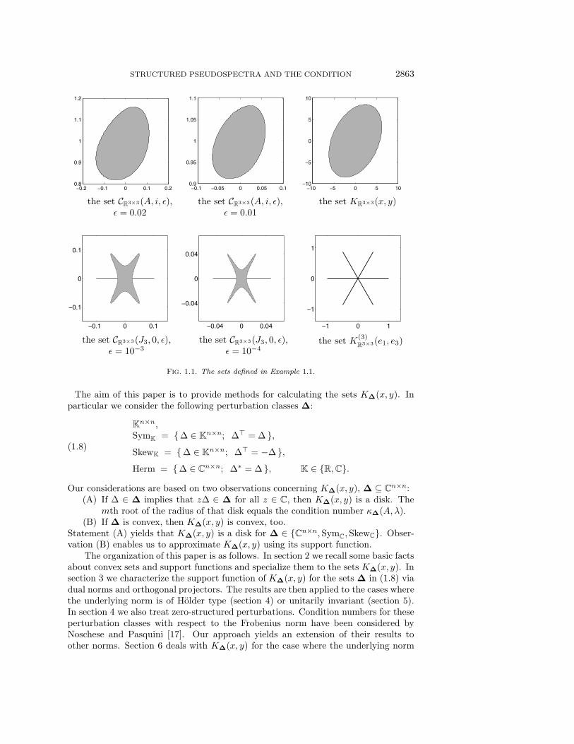
Example 1.1. The relation (1.7) is illustrated in Figure 1.1. The underlying normin the following explanation is the spectral norm.

The upper row of the figure deals with the case m = 1. The first two picturesshow the sets CR3×3(A, λ, ε) for the matrix

A =

⎡⎣−3 −10 −101 5 50 −2 −2

⎤⎦and its simple eigenvalue λ = i. A corresponding pair of right and left eigenvectorssatisfying y∗x = 1 is given by

x = [1 + 3i − 2− i 2]�, y = (1/2)[1 3− i 3− i]�.

The right picture in the upper row shows the set K(1)Rn×n(x, y) = KRn×n(x, y). By (1.7)

we have

limε→0

CR3×3(A, i, ε)− i

ε= KR3×3(x, y).

The pictures indicate the convergence. The scalings have been chosen such that thedisplayed sets have approximately the same size. The plots of the pseudospectracomponents CR3×3(A, i, ε) have been generated using the formula

σRn×n(A, ε) = { s ∈ C; τn(sI −A) ≤ ε }, A ∈ Cn×n, ε > 0.

Here τn denotes the smallest real perturbation value of the second kind [1], whichis given by

τn(M) = supγ∈(0,1]

σ2n−1

([ �M −γ �Mγ−1 �M �M

]), M ∈ C

n×n,

where σ2n−1 is the second smallest singular value. The set KR3×3(x, y) has beencomputed using Theorem 6.5 below.

The left pictures in the lower row of the figure show the real pseudospectraσR3×3(J3, ε) = CR3×3(J3, 0, ε) for the 3 by 3 Jordan block

J3 =

⎡⎣0 1 00 0 10 0 0

⎤⎦ .

The right picture shows the limit set K(3)Rn×n(e1, e3), where e1 = [1 0 0]�, e3 = [0 0 1]�.

Note that e1 is a right eigenvector and e∗1 is a left generalized eigenvector of J3satisfying e∗1e1 = 1, e∗1J

23 = e∗3. Hence, (1.7) yields

limε→0

CR3×3(J3, 0, ε)

ε1/3= K

(3)R3×3(e1, e3).

It is easily verified that the set KR3×3(e1, e3) equals the interval [−1, 1]. Thus,

K(3)R3×3(e3, e1) = [−1, 1] ∪ eπi/3[−1, 1] ∪ e2πi/3[−1, 1].


−0.2 −0.1 0 0.1 0.20.8

0.9

1

1.1

1.2

−0.1 −0.05 0 0.05 0.10.9

0.95

1

1.05

1.1

−10 −5 0 5 10−10

−5

0

5

10

the set CR3×3(A, i, ε),ε = 0.02

the set CR3×3(A, i, ε),ε = 0.01

the set KR3×3(x, y)

−0.1 0 0.1

−0.1

0

0.1

−0.04 0 0.04

−0.04

0

0.04

−1 0 1

−1

0

1

the set CR3×3(J3, 0, ε),ε = 10−3

the set CR3×3(J3, 0, ε),ε = 10−4

the set K(3)R3×3(e1, e3)

Fig. 1.1. The sets defined in Example 1.1.

The aim of this paper is to provide methods for calculating the sets KΔ(x, y). Inparticular we consider the following perturbation classes Δ:

Kn×n,SymK = {Δ ∈ Kn×n; Δ� = Δ },SkewK = {Δ ∈ Kn×n; Δ� = −Δ },Herm = {Δ ∈ C

n×n; Δ∗ = Δ }, K ∈ {R,C}.

(1.8)

Our considerations are based on two observations concerning KΔ(x, y), Δ ⊆ Cn×n:(A) If Δ ∈ Δ implies that zΔ ∈ Δ for all z ∈ C, then KΔ(x, y) is a disk. The

mth root of the radius of that disk equals the condition number κΔ(A, λ).(B) If Δ is convex, then KΔ(x, y) is convex, too.

Statement (A) yields that KΔ(x, y) is a disk for Δ ∈ {Cn×n, SymC, SkewC}. Obser-vation (B) enables us to approximate KΔ(x, y) using its support function.

The organization of this paper is as follows. In section 2 we recall some basic factsabout convex sets and support functions and specialize them to the sets KΔ(x, y). Insection 3 we characterize the support function of KΔ(x, y) for the sets Δ in (1.8) viadual norms and orthogonal projectors. The results are then applied to the cases wherethe underlying norm is of Holder type (section 4) or unitarily invariant (section 5).In section 4 we also treat zero-structured perturbations. Condition numbers for theseperturbation classes with respect to the Frobenius norm have been considered byNoschese and Pasquini [17]. Our approach yields an extension of their results toother norms. Section 6 deals with KΔ(x, y) for the case where the underlying norm

2864 MICHAEL KAROW

is either the spectral norm or the Frobenius norm. It is shown that KΔ(x, y) is anellipse for many important perturbation classes. The results obtained so far will beextended in section 7 to classes of matrices that are self- or skew-adjoint with respectto an inner product.

2. Characterization by support functions. Let K be a nonempty compactconvex subset of C. Then its support function sK : C → R is defined by

sK(z) = maxξ∈K

�(z ξ) = maxξ∈K

z�ξ,(2.1)

where in the second equation the complex numbers z = z1 + iz2, ξ = ξ1 + iξ2 havebeen identified with the corresponding vectors [z1, z2]

�, [ξ1, ξ2]� ∈ R2. The set K isuniquely determined by its support function since we have [9, Corollary 3.1.2]

K = {ξ ∈ C; �(z ξ) ≤ sK(z) for all z ∈ C with |z| = 1}.(2.2)

Furthermore, the boundary of K is given as

∂K = {ξ ∈ K; �(z ξ) = sK(z) for some z ∈ C with |z| = 1}.(2.3)

This follows from (2.2) and the compactness of the unit circle. Let rK = max{ |ξ|; ξ ∈K }. Then rK is the radius of the smallest disk about 0 that contains K. It is easilyseen that rK = max{sK(z); z ∈ C, |z| = 1 }. If sK(z) = r |z| for some r ≥ 0, then Kis a disk about 0 with radius r = rK . We will also need the following fact.

Proposition 2.1. Assume the nonempty compact convex set K ⊂ C is pointsymmetric with respect to 0; i.e., ξ ∈ K implies −ξ ∈ K. Assume further thatsK(z) = 0 for some z ∈ C with |z| = 1. Then K is a line segment. Specifically,

K = { θ iz; θ ∈ R, |θ| ≤ sK(iz) }.Proof. From the point symmetry it follows that sK(z) = sK(−z). Hence, if

sK(z) = 0, then �(z ξ) = 0 for all ξ ∈ K. Thus K ⊂ { θ iz; θ ∈ R}. By compactnessand convexity, K = { θ iz; θ ∈ R, |θ| ≤ r } for some r ≥ 0. It is easily verified thatr = sK(iz) if |z| = 1.

The relations (2.2) and (2.3) can be used to approximate K via the followingmethod (adapted from the standard algorithm for approximating the boundary of thefield of values [11, section 1.5]). Let zj = eiφj , j ∈ N , where 0 = φ1 < φ2 < · · · <φN < 2π. Let ξj ∈ K, j ∈ N, be such that �(zj ξj) = sK(zj). Then by (2.3) eachξj is a boundary point of K. Let K1 denote the convex hull of these points, and letK2 = {ξ ∈ C; �(zjξ) ≤ sK(zj), j ∈ N }. Then we have K1 ⊆ K ⊆ K2, where thelatter inclusion follows from (2.2). The boundary of K1 is a polygon with verticesξ1, ξ2, . . . , ξN .

The proposition below yields the basis for our further development.Proposition 2.2. Let Δ be a nonempty convex subset of C

n×n. Then thefollowing hold:

(i) The set KΔ(x, y) defined in (1.1) is a compact convex subset of C with supportfunction

sΔ(z) = maxΔ ∈ Δ‖Δ‖ ≤ 1

�(z y∗Δx) = maxΔ ∈ Δ‖Δ‖ ≤ 1

� tr(Δ∗(z yx∗)), z ∈ C.(2.4)

If Δ is a cone, then the maximum is attained for some Δ ∈ Δ with‖Δ‖ = 1.


(ii) Let |z| = 1, and let Δz ∈ Δ be a maximizer for (2.4). Then y∗Δzx is aboundary point of KΔ(x, y).

(iii) Suppose Δ is a vector space over R, and let sΔ(z) = 0 for some z ∈ C with|z| = 1. Then KΔ(x, y) is a line segment. Specifically,

KΔ(x, y) = { θ iz; θ ∈ R, |θ| ≤ sΔ(iz) }.Proof. The compactness and convexity of KΔ(x, y) are obvious. Equation (2.4)

is immediate from (2.1) and the relations

z y∗Δx = tr(z y∗Δx) = tr(z xy∗Δ) = tr((z yx∗)∗Δ) = tr(Δ∗(z yx∗)).

(ii) follows from (2.3). (iii) is a consequence of Proposition 2.1.

3. Dual norms and orthogonal projectors. The dual of a vector norm ‖ · ‖ :Cn → R is defined by

‖x‖′ = maxy ∈ C

n

‖y‖ = 1

�(y∗x), x ∈ Cn.(3.1)

There is a natural extension of this definition to matrix norms.Definition 3.1. Let ‖ · ‖ be a norm on Cn×n. Then its dual is defined as

‖X‖′ := maxY ∈ C

n×n

‖Y ‖ = 1

� tr(Y ∗X), X ∈ Cn×n.(3.2)

This yields the following corollary to Proposition 2.2.Corollary 3.2. For any norm ‖ · ‖ on Cn×n the support function sCn×n of

KCn×n(x, y) is given by sCn×n(z) = |z| ‖yx∗‖′, z ∈ C. Thus KCn×n(x, y) is a disk ofradius ‖yx∗‖′.

The map

(X,Y ) → � tr(Y ∗X)(3.3)

is a positive definite symmetric R-bilinear form on Cn×n. Thus for each subspace(over R) Δ ⊆ Cn×n we have the direct decomposition Cn×n = Δ ⊕ Δ⊥, whereΔ⊥ = {X ∈ Cn×n; � tr(Δ∗X) = 0 for all Δ ∈ Δ } is the orthogonal complement ofΔ with respect to the inner product (3.3). The orthogonal projector onto Δ is theR-linear map PΔ : Cn×n → Cn×n satisfying

PΔ(X1 +X2) = X1 for all X1 ∈ Δ, X2 ∈ Δ⊥.

Note that for all X,Y ∈ Cn×n,

� tr(PΔ(Y )∗X) = � tr(PΔ(Y )∗PΔ(X)) = � tr(Y ∗PΔ(X)).(3.4)

We will need the following lemma.Lemma 3.3. Let Δ ⊆ Cn×n be a vector space over C, and let ΔR = Δ ∩ Rn×n.

Suppose that Δ = ΔR ⊕ iΔR. Then the orthogonal projector onto ΔR satisfies

PΔR(X) = �(PΔ(X)) for all X ∈ C

n×n.(3.5)

Proof. This is immediate from the fact that the vector spaces ΔR and iΔR areorthogonal to each other with respect to the inner product (3.3).

2866 MICHAEL KAROW

The table below gives the orthogonal projectors for the subspaces introduced in(1.8):

Δ PΔ(X)

Cn×n X

Rn×n �XHerm (X +X∗)/2

SymC (X +X�)/2

SkewC (X −X�)/2

SymR �(X +X�)/2

SkewR �(X −X�)/2

(3.6)

The main results of this paper are based on the next lemma.Lemma 3.4. Let ‖ · ‖ be a norm on Cn×n, and let Δ ⊆ Cn×n be a vector space

over R. Suppose the orthogonal projector onto Δ is a contraction with respect to thenorm ‖ · ‖, i.e.,

‖PΔ(X)‖ ≤ ‖X‖ for all X ∈ Cn×n.(3.7)

Then, for all M ∈ Cn×n,

maxΔ ∈ Δ‖Δ‖ = 1

� tr(Δ∗M) = ‖PΔ(M)‖′.(3.8)

Let Δ0 ∈ Cn×n be such that ‖Δ0‖ = 1, and let � tr(Δ∗0 PΔ(M)) = ‖PΔ(M)‖′. If

PΔ(M) = 0, then the matrix Δ1 = PΔ(Δ0) is a maximizer for the left-hand side of(3.8).

Proof. Let L denote the left-hand side of (3.8). For Δ ∈ Δ we have � tr(Δ∗M) =� tr(Δ∗PΔ(M)). This yields L ≤ ‖PΔ(M)‖′. We show the opposite inequality. Forthe matrix Δ0 we have ‖PΔ(M)‖′ = � tr(Δ∗

0PΔ(M)) = � tr(PΔ(Δ0)∗PΔ(M)). If

PΔ(Δ0) = 0, then ‖PΔ(M)‖′ = 0 = L. Suppose PΔ(Δ0) = 0. By condition (3.7) wehave ‖PΔ(Δ0)‖ ≤ ‖Δ0‖ = 1. The matrix Δ1 = PΔ(Δ0)/‖PΔ(Δ0)‖ satisfies ‖Δ1‖ =1 and � tr(Δ∗

1PΔ(M)) = ‖PΔ(M)‖′/‖PΔ(Δ0)‖ ≥ ‖PΔ(M)‖′. Thus L ≥ ‖PΔ(M)‖′.Consequently, L = ‖PΔ(M)‖′ and ‖PΔ(Δ0)‖ = 1.

Remark 3.5. The Frobenius norm ‖X‖F =√tr(X∗X) is the norm induced by

the inner product (X,Y ) → � tr(X∗Y ). Hence, the Frobenius norm is its own dual,and an orthogonal projection onto a subspace (over R or C) is always a contractionwith respect to the Frobenius norm. Thus, all statements of Lemma 3.4 hold for‖ · ‖ = ‖ · ‖F , and we have ‖PΔ(M)‖′F = ‖PΔ(M)‖F .

From Proposition 2.2 and Lemma 3.4 (applied to the matrix M = z yx∗, z ∈ C)we obtain the following theorem.

Theorem 3.6. Let Δ ⊆ Cn×n be a vector space over R, and let sΔ : C → R

denote the support function of KΔ(x, y). Suppose (3.7) holds for the underlying norm.Then the following hold:

(i) The support function satisfies

sΔ(z) = ‖PΔ(z yx∗)‖′, z ∈ C.(3.9)


(ii) Let |z| = 1, and let Δz ∈ Cn×n be such that ‖Δz‖ = 1 and � tr(Δ∗zPΔ(z yx∗)) =

sΔ(z). Then y∗PΔ(Δz)x ∈ C is a boundary point of KΔ(x, y). If y∗PΔ(Δz)x =0, then KΔ(x, y) is a line segment.

(iii) If Δ is a vector space over C, then

sΔ(z) = ‖PΔ(yx∗)‖′ |z|, z ∈ C.(3.10)

Thus KΔ(x, y) is a disk about 0 with radius ‖PΔ(yx∗)‖′.Next, we consider norms that have one of the following properties (a)–(c) for all

X ∈ Cn×n:

(3.11) (a) ‖X‖ = ‖X‖, (b) ‖X‖ = ‖X∗‖, (c) ‖X‖ = ‖X�‖.Note that two of these conditions imply the third.

Lemma 3.7. Let Δ ⊆ Cn×n be a vector space over C such that Δ = ΔR ⊕ iΔR,where ΔR = Δ ∩ Rn×n. Let ‖ · ‖ be a norm such that conditions (a) and (3.7) hold.Then condition (3.7) also holds for the orthogonal projector onto ΔR; i.e., we have‖PΔR

(X)‖ ≤ ‖X‖ for all X ∈ Cn×n.Proof. We have, for X ∈ Cn×n,

‖PΔR(X)‖ = ‖�(PΔ(X))‖ (by Lemma 3.3)

=1

2‖PΔ(X) + PΔ(X)‖

≤ 1

2(‖PΔ(X)‖+ ‖PΔ(X)‖)

= ‖PΔ(X)‖ (by condition (a))

≤ ‖X‖.Lemma 3.8. Condition (3.7) holds for the following cases:(i) The norm satisfies (a) and Δ = Rn×n.(ii) The norm satisfies (b) and Δ = Herm.(iii) The norm satisfies (c) and Δ ∈ {SymC, SkewC}.(iv) The norm satisfies (a), (b), and (c) and Δ ∈ {SymR, SkewR}.Proof. (i) is immediate from Lemma 3.7. (b) implies that ‖PHerm(X)‖ = ‖(X +

X∗)/2‖ ≤ (‖X‖ + ‖X∗‖)/2 = ‖X‖. This yields (ii). The proof of (iii) is analogous.(iv) follows from (iii) and Lemma 3.7.

Theorem 3.9. The following assertions hold for the support function sΔ : C → R

of KΔ(x, y):(i) If the norm ‖ · ‖ satisfies condition (a), then sRn×n(z) = ‖�(z yx∗)‖′.(ii) If the norm ‖ · ‖ satisfies condition (b), then sHerm(z) = ‖PHerm(z yx

∗)‖′.(iii) If the norm ‖ · ‖ satisfies condition (c), then

sSymC(z) = ‖PSym

C(z yx∗)‖′ = ‖PSym

C(yx∗)‖′ |z|

and

sSkewC(z) = ‖PSkewC

(z yx∗)‖′ = ‖PSkewC(yx∗)‖′ |z|.

(iv) If the norm ‖ · ‖ satisfies (a), (b), and (c), then

sSymR(z) = ‖PSym

R(z yx∗)‖′ and sSkewR

(z) = ‖PSkewR(z yx∗)‖′.

In the next sections we specialize Theorem 3.9 to classes of norms for which theduals can be explicitly given.

2868 MICHAEL KAROW

4. Norms of Holder type. The Holder-p-norm of x = [x1, . . . , xn]� ∈ Cn is

defined by

‖x‖p =

⎧⎨⎩(∑

j∈n |xj |p)1/p

for 1 ≤ p < ∞,

maxj∈n |xj | for p = ∞.(4.1)

We consider the matrix norms of Holder type [8, page 717] defined by

‖X‖r|p =∥∥∥ [ ‖x�

1 ‖r, . . . , ‖x�n ‖r

]� ∥∥∥p, 1 ≤ p, r ≤ ∞,(4.2)

where x1, . . . , xn denote the rows of X ∈ Cn×n. Note that ‖X‖1|∞ is the row sumnorm and

‖X‖p|p =

⎧⎨⎩(∑

j,k∈n |xjk|p)1/p

for 1 ≤ p < ∞,

maxj,k∈n |xjk| for p = ∞,(4.3)

where the numbers xjk are the entries of X . In particular, ‖ · ‖2|2 is the Frobeniusnorm.

As is well known the dual of the Holder-p-norm is the Holder-q-norm, where1p + 1

q = 1 if 1 ≤ p < ∞ and q = 1 if p = ∞. Using this fact the next proposition iseasily verified.

Proposition 4.1. The dual of the norm ‖ · ‖r|p is ‖ · ‖t|q, where1r + 1

t = 1 if 1 ≤ r < ∞ and t = 1 if r = ∞,

1p + 1

q = 1 if 1 ≤ p < ∞ and q = 1 if p = ∞.(4.4)

To a given X ∈ Cn×n with rows x1, . . . , xn a matrix Y0 ∈ Cn×n satisfying ‖Y0‖t|q = 1and � tr(Y ∗

0 X) = � tr(XY ∗0 ) = ‖X‖r|p can be constructed via the following procedure.

Let ξ = [ ‖x�1 ‖r, . . . , ‖x�

n ‖r ]�. Choose a nonnegative vector η = [ η1, . . . , ηn]� such

that ‖η‖q = 1 and η�ξ = ‖ξ‖p. For each j ∈ n choose a row vector yj ∈ Cn

with ‖y�j ‖t = ηj and xjy�j = ‖x�

j ‖r ηj. Then Y0 = [ y�1 , . . . , y�n ]∗ has the required

properties.From Proposition 4.1 combined with Corollary 3.2 and Theorem 3.9 we get the

following corollary.Corollary 4.2. Let 1 ≤ r, p ≤ ∞, and let t, q be given by (4.4). Let KΔ(x, y) =

{ y∗Δx; Δ ∈ Δ, ‖Δ‖r|p ≤ 1}. Then the following hold:(i) the set KCn×n(x, y) is a disk of radius ‖yx∗‖t|q;(ii) the support function of KRn×n(x, y) is

sRn×n(z) = ‖�(z yx∗)‖t|q, z ∈ C;

(iii) for the case p = r and Δ ∈ {Herm, SymC, SkewC, SymR, SkewR} the supportfunction of KΔ(x, y) is sΔ(z) = ‖PΔ(z yx∗)‖q|q.

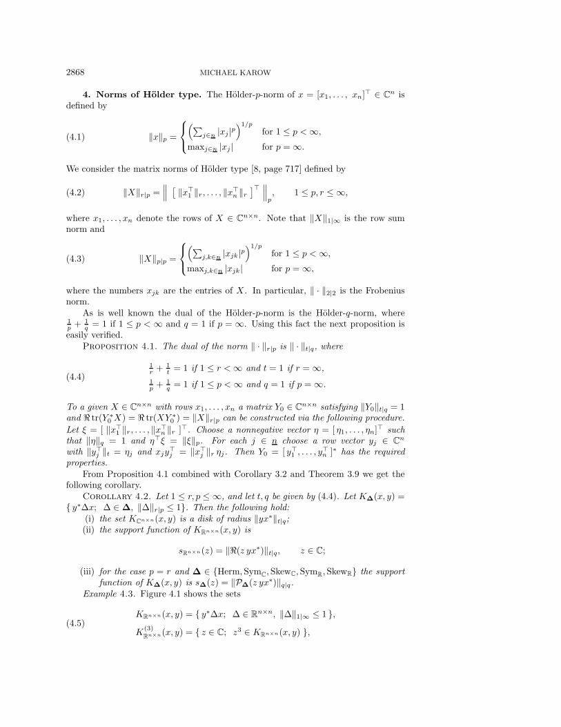
Example 4.3. Figure 4.1 shows the sets

KRn×n(x, y) = { y∗Δx; Δ ∈ Rn×n, ‖Δ‖1|∞ ≤ 1 },K

(3)Rn×n(x, y) = { z ∈ C; z3 ∈ KRn×n(x, y) },

(4.5)


−20 0 20

−20

0

20

−2 0 2

−2

0

2

Fig. 4.1. The sets KRn×n(x, y) (left) and K

(3)

Rn×n(x, y) (right) from Example 4.3.

where

x = [ 1− i, −4, 1 ]�, y = [ 2− i, 2, 2− i ]�.

The plot of KRn×n(x, y) has been generated by computing 200 boundary points usingclaim (ii) of Theorem 3.6 and Proposition 4.1.

The following theorem extends a result by Noschese and Pasquini [17] on zero-structured perturbations.

Theorem 4.4. For an index set I ⊆ n × n, let Δ(I) denote the set of Δ =[δjk] ∈ Cn×n with δjk = 0 for (j, k) ∈ I.

(i) The orthogonal projection of X = [xjk] ∈ Cn×n onto Δ(I) is given by

PΔ(I)(X) = [xjk ], where xjk =

{xjk if (j, k) ∈ I,0 if (j, k) ∈ I.(4.6)

The orthogonal projection onto Δ(I) ∩ Rn×n satisfies

PΔ(I)∩Rn×n(X) = �(PΔ(I)(X)) = [xjk],(4.7)

where

xjk =

{�xjk if (j, k) ∈ I,0 if (j, k) ∈ I.

(ii) Let p, q ∈ [1,∞] be such that 1p + 1

q = 1. Then the support function of

KΔ(I)(x, y) = {y∗Δx; Δ ∈ Δ(I), ‖Δ‖p|p ≤ 1} is given by

sΔ(I)(z) = ‖PΔ(I)(z yx∗)‖q|q = ‖PΔ(I)(yx∗)‖q|q |z|, z ∈ C.

Hence KΔ(I)(x, y) is a disk about 0 of radius ‖PΔ(I)(yx∗)‖q|q. Further-more, the support function of KΔ(I)∩Rn×n(x, y) = {y∗Δx; Δ ∈ Δ(I) ∩Rn×n, ‖Δ‖p|p ≤ 1} is given by

sΔ(I)∩Rn×n(z) = ‖PΔ(I)∩Rn×n(z yx∗)‖q|q = ‖�(z PΔ(I)(yx∗))‖q|q, z ∈ C.

Proof. Obviously, the orthogonal complement of Δ(I) is Δ((n × n) \ I). Thisyields (4.6). Equation (4.7) follows from Lemma 3.3. It is easily seen that the pro-jectors in (i) satisfy the contraction condition (3.7) for ‖ · ‖ = ‖ · ‖p|p. This yields(ii).

2870 MICHAEL KAROW

5. Unitarily invariant norms. In what follows, Un denotes the set of all uni-tary n × n matrices. A norm ‖ · ‖ on Cn×n is said to be unitarily invariant if‖UXV ‖ = ‖X‖ for all X ∈ Cn×n, U, V ∈ Un. There is a one to one correspon-dence between the unitarily invariant norms on Cn×n and symmetric gauge functions[22, section II.3]. A symmetric gauge function Φ is a symmetric and absolute normon Rn. The unitarily invariant norm ‖ · ‖Φ associated with Φ is given by

‖X‖Φ := Φ([σ1(X), σ2(X), . . . , σn(X)]�),(5.1)

where σ1(X) ≥ σ2(X) ≥ · · · ≥ σn(X) denote the singular values of X ∈ Cn×n. Theunitarily invariant norm induced by the Holder-p-norm is called the Schatten-p-norm,which we denote by

‖X‖(p) :=⎧⎨⎩(∑

k∈n σk(X)p)1/p

if 1 ≤ p < ∞,

σ1(X) if p = ∞.

Note that ‖X‖(∞) is the spectral norm and ‖X‖(2) =√tr(X∗X) is the Frobenius

norm of X . In the following, Φ′ stands for the dual of the symmetric gauge functionΦ, i.e.,

Φ′(ξ) = maxη ∈ R

n

Φ(η) = 1

η�ξ, ξ ∈ Rn.(5.2)

Let X = Udiag(σ)V ∗ be a singular value decomposition, where U, V ∈ Un and σ =[σ1, . . . , σn]

� is the vector of singular values of X ∈ Cn×n. Let τ = [τ1, . . . , τn]� be

a nonnegative vector such that Φ(τ) = 1 and τ�σ = Φ′(σ). Let Y0 = Udiag(τ)V ∗.Then

‖X‖′Φ = maxY ∈ C

n×n

‖Y ‖Φ = 1

� tr(Y ∗X) ≥ � tr(Y ∗0 X) = τ�σ = Φ′(σ) = ‖X‖Φ′.(5.3)

It can be shown that the inequality in (5.3) is actually an equality. Hence we havethe following result [2, Proposition IV.2.11].

Proposition 5.1. For any symmetric gauge function Φ the dual of the unitarilyinvariant norm ‖ · ‖Φ is ‖ · ‖Φ′ .

From (5.1) it follows that unitarily invariant norms have properties (a), (b), and(c) of (3.11). Thus, by combining Theorem 3.9 and Proposition 5.1, we get thefollowing result.

Theorem 5.2. Let Φ be a symmetric gauge function on Rn, and let Δ be one ofthe sets in (3.6). Then the support function of

KΔ(x, y) = { y∗Δx; Δ ∈ Δ, ‖Δ‖Φ ≤ 1}, x, y ∈ Cn,

is given by

sΔ(z) = ‖PΔ(z yx∗)‖Φ′ = Φ′( [σ1(z), . . . , σn(z)]� ), z ∈ C,

where σ1(z), . . . , σn(z) denote the singular values of PΔ(z yx∗).


6. Frobenius norm and spectral norm. The results in this section are basedon the following proposition about the support function of an ellipse.

Proposition 6.1. Let K ⊂ C be a nonempty compact convex set with supportfunction

sK(z) =√a |z|2 + �(b z2), z, b ∈ C, a ≥ |b|.

Then K is an ellipse (which may degenerate to a line segment). Specifically,

K ={e−iφ/2

(√a+ |b| ξ1 +

√a− |b| ξ2 i

); ξ1, ξ2 ∈ R, ξ21 + ξ22 ≤ 1

},(6.1)

where φ = arg(b).

Proof. Let E denote the set on the right-hand side of (6.1), and let sE denote itssupport function. Let

α =1

2(√

a+ |b|+√a− |b|) e−iφ/2, β =

1

2(√a+ |b| −

√a− |b|) e−iφ/2.

Then, for ξ1, ξ2 ∈ R,

e−iφ/2(√

a+ |b| ξ1 +√a− |b| ξ2 i

)= αξ + βξ, where ξ = ξ1 + ξ2 i ∈ C.

Thus

sE(z) = max|ξ|≤1

�(z (α ξ + β ξ))

= max|ξ|≤1

�( (α z + β z) ξ)

= |α z + β z|=

√(|α|2 + |β|2)|z|2 + 2�(z2 αβ)

=√a |z|2 + �(z2 b).

Thus sE = sK , and consequently E = K.

Note that the set (6.1) is a disk if b = 0 and a > 0. It is a line segment ifa = |b| > 0.

The next theorem characterizes the sets KΔ(x, y) if the underlying norm is theFrobenius norm ‖ · ‖F .

Theorem 6.2. Let x, y ∈ Cn, and let P = PΔ(yx∗). Furthermore, let Δ ⊆ Cn×n

be a vector space over C. Then the following hold:

(i) The set KΔ(x, y) = { y∗Δx; Δ ∈ Δ, ‖Δ‖F ≤ 1} is a disk about 0 of radius‖P‖F .

(ii) Suppose that Δ = ΔR ⊕ iΔR, where ΔR = Δ ∩ Rn×n. Then the set

KΔR(x, y) = {y∗Δx; Δ ∈ ΔR, ‖Δ‖F ≤ 1} equals the ellipse defined in

(6.1) with

a =1

2tr(P ∗P ) =

1

2‖P‖2F , b =

1

2tr(P�P ).

Proof. (i) is a special case of claim (iii) of Theorem 3.6.

2872 MICHAEL KAROW

(ii) The support function of KΔR(x, y) satisfies

sΔR(z) = ‖PΔR

(z yx∗)‖(2) (by claim (i) of Theorem 3.9)

= ‖�(zP )‖(2) (by Lemma 3.3)

=1

2‖zP + zP‖(2)

=1

2

√tr((zP + zP )∗(zP + zP ))

=1

2( |z|2(tr(P ∗P ) + tr(P ∗P )︸︷︷︸

=2tr(P∗P )

) + z2tr(P ∗P ) + z2tr(P ∗P )︸︷︷︸=2 (z2 tr(P�P ))

)1/2

=√a |z|2 + �(b z2).

Now, (ii) follows from Proposition 6.1.Theorem 6.2 has the following consequences for structured eigenvalue condition

numbers.Corollary 6.3. Let λ ∈ C be a simple eigenvalue of A ∈ Cn×n with right

eigenvector x ∈ Cn and left eigenvector y ∈ Cn such that y∗x = 1. Then the followingstatements hold for the structured condition number

(6.2) κΔ(A, λ) = max{ |y∗Δx|; Δ ∈ Δ, ‖Δ‖ ≤ 1 }.

(i) If the set KΔ(x, y) = {y∗Δx; Δ ∈ Δ, ‖Δ‖ ≤ 1} equals the ellipse in (6.1),then

κΔ(A, λ) =√a+ |b|.

(ii) Suppose the norm in (6.2) is the Frobenius norm. Let Δ ⊆ Cn×n be a subspaceover C, and let P = PΔ(yx∗) denote the orthogonal projection of yx∗ ontoΔ. Then

(6.3) κΔ(A, λ) = ‖P‖F .

Suppose additionally that Δ = ΔR ⊕ iΔR, where ΔR = Δ ∩ Rn×n. Then

(6.4) κΔR(A, λ) =

√1

2‖P‖2F +

1

2|tr(PTP )|.

In particular, the following inequality holds:

κΔR(A, λ) ≥ 1√

2κΔ(A, λ).

Proof. (i) is obvious and (ii) is a consequence of (i) and Theorem 6.2.Remark 6.4. Relation (6.3) is Tisseur’s formula [23, section 4] in another notation.

From (6.3) one obtains the results of Noschese and Pasquini [18] on the structuredcondition number of Toeplitz matrices by observing that the orthogonal projection ofa matrix X ∈ Cn×n onto the set of Toeplitz matrices is given by replacing the entriesin each diagonal of X by their arithmetic mean.

Relation (6.4) generalizes a result by Byers and Kressner [4] on condition numberswith respect to real perturbations.


The next theorem gives explicit formulae for the constants a and b if Δ is oneof the perturbation classes defined in (1.8). Here we also consider the case where theunderlying norm is the spectral norm.

Theorem 6.5. Let ‖Δ‖ denote either the Frobenius norm or the spectral normof Δ ∈ C

n×n. Let Δ ⊆ Cn×n, and let a ≥ 0, b ∈ C be as in the tables below. Then

the support function of

KΔ(x, y) = { y∗Δx; Δ ∈ Δ, ‖Δ‖ ≤ 1}is given by

sΔ(z) =√a |z|2 + �(b z2), z ∈ C.(6.5)

Hence, KΔ(x, y) equals the ellipse defined in (6.1).

Table for the Frobenius norm:

Δ a b

Cn×n ‖x‖2‖y‖2 0

Rn×n 12‖x‖2‖y‖2 1

2(x�x) (y�y)

Herm 12‖x‖2‖y‖2 1

2(x∗y)2

SymC12(‖x‖2‖y‖2 + |x�y|2) 0

SkewC12(‖x‖2‖y‖2 − |x�y|2) 0

SymR14(‖x‖2‖y‖2 + |x�y|2) 1

4( (x�x) (y�y) + (x∗y)2)

SkewR14(‖x‖2‖y‖2 − |x�y|2) 1

4( (x�x) (y�y)− (x∗y)2)

Table for the spectral norm:

Δ a b

Cn×n ‖x‖2‖y‖2 0

Rn×n 12

[‖x‖2 ‖y‖2 +

√(‖x‖4 − |x�x|2)(‖y‖4 − |y�y|2)

]12(x�x)(y�y)

Herm ‖x‖2‖y‖2 − 12|y∗x|2 1

2(x∗y)2

SymC ‖x‖2‖y‖2 0

SkewC ‖x‖2‖y‖2 − |x�y|2 0

SkewR12( ‖x‖2‖y‖2 − |x�y|2 +

√det(F ∗F ) ) 1

2((x�x)(y�y)− (x∗y)2)

F =[x x y y

]

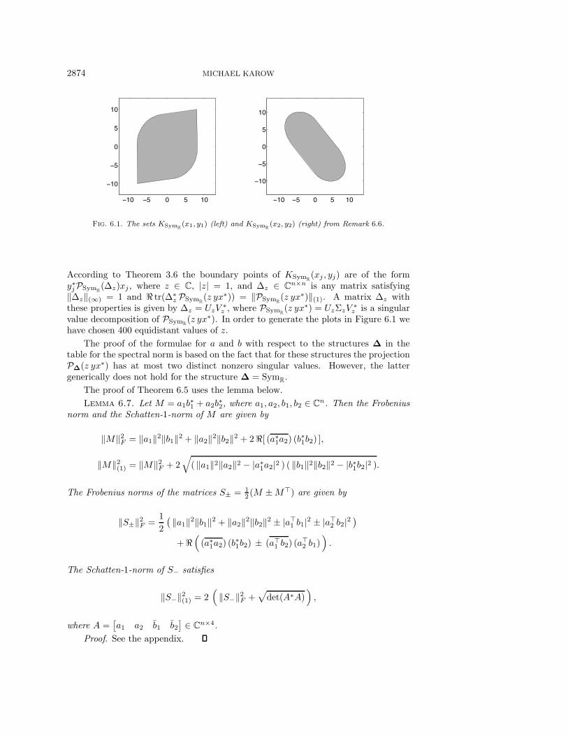
Here and in the following, ‖x‖, ‖y‖ denote the Euclidean norm of x, y ∈ Cn.Remark 6.6. Theorem 6.5 makes no statement about the case where Δ = SymR

and the underlying norm is the spectral norm. The associated sets KSymR(x, y) are in

general not ellipses. Figure 6.1 gives two examples. It shows the sets KSymR(xj , yj),

j = 1, 2, where

x1 = [2 + i, 2 + i, 2]�, y1 = [−2, −2, 3i]�,

x2 = [1 + 2i, i, 2]�, y2 = [i, −2 + 2i, 1 + 2i]�.(6.6)

2874 MICHAEL KAROW

−10 −5 0 5 10

−10

−5

0

5

10

−10 −5 0 5 10

−10

−5

0

5

10

Fig. 6.1. The sets KSymR(x1, y1) (left) and KSymR

(x2, y2) (right) from Remark 6.6.

According to Theorem 3.6 the boundary points of KSymR(xj , yj) are of the form

y∗jPSymR(Δz)xj , where z ∈ C, |z| = 1, and Δz ∈ Cn×n is any matrix satisfying

‖Δz‖(∞) = 1 and � tr(Δ∗z PSym

R(z yx∗)) = ‖PSym

R(z yx∗)‖(1). A matrix Δz with

these properties is given by Δz = UzV∗z , where PSym

R(z yx∗) = UzΣzV

∗z is a singular

value decomposition of PSymR(z yx∗). In order to generate the plots in Figure 6.1 we

have chosen 400 equidistant values of z.

The proof of the formulae for a and b with respect to the structures Δ in thetable for the spectral norm is based on the fact that for these structures the projectionPΔ(z yx∗) has at most two distinct nonzero singular values. However, the lattergenerically does not hold for the structure Δ = SymR.

The proof of Theorem 6.5 uses the lemma below.

Lemma 6.7. Let M = a1b∗1 + a2b

∗2, where a1, a2, b1, b2 ∈ Cn. Then the Frobenius

norm and the Schatten-1-norm of M are given by

‖M‖2F = ‖a1‖2‖b1‖2 + ‖a2‖2‖b2‖2 + 2�[ (a∗1a2) (b∗1b2) ],

‖M‖2(1) = ‖M‖2F + 2√( ‖a1‖2‖a2‖2 − |a∗1a2|2 ) ( ‖b1‖2‖b2‖2 − |b∗1b2|2 ).

The Frobenius norms of the matrices S± = 12 (M ±M�) are given by

‖S±‖2F =1

2

( ‖a1‖2‖b1‖2 + ‖a2‖2‖b2‖2 ± |a�1 b1|2 ± |a�2 b2|2)

+�((a∗1a2) (b

∗1b2) ± (a�1 b2) (a

�2 b1)

).

The Schatten-1-norm of S− satisfies

‖S−‖2(1) = 2(‖S−‖2F +

√det(A∗A)

),

where A =[a1 a2 b1 b2

] ∈ Cn×4.

Proof. See the appendix.


Proof of Theorem 6.5. First, we treat the case where Δ = Rn×n. Let

Mz = 2�(z y x∗) = z y x∗ + z y x∗.

According to Proposition 5.1 the dual of the spectral norm is the Schatten-1-norm.Hence, by Theorem 5.2 the support function of KRn×n(x, y) (with respect to spectralnorm) is

sRn×n(z) = ‖PRn×n(z yx∗)‖(1) (by Theorem 5.2)

= ‖�(z yx∗)‖(1)=

1

2‖Mz‖(1)

=1

2

√αz + 2

√βz (by Lemma 6.7),

where

αz = ‖Mz‖2F= ‖z y‖2‖x‖2 + ‖z y‖2‖x‖2 + 2�[ ((z y)∗(z y)) (x∗x) ]

= 2 (|z|2‖x‖2‖y‖2 + �[z2(x�x) (y�y)]),

βz = ( ‖z y‖2‖zy‖2 − |(z y)∗(z y)|2 ) ( ‖x‖2‖x‖2 − |x∗x|2 )= |z|4(‖x‖4 − |x�x|2)(‖y‖4 − |y�y|2).

If the underlying norm is the Frobenius norm, then

sRn×n(z) = ‖�(z yx∗)‖F =1

2‖Mz‖F =

1

2

√αz.

Next, we consider the real skew-symmetric case. Let S− = 12 (Mz−M�

z ). The supportfunction of KSkewR

(x, y) with respect to the spectral norm is

sSkewR(z) = ‖PSkewR

(z yx∗)‖(1) (by Theorem 5.2)

=1

2‖S−‖(1)

=1

2

√2 ‖S−‖2F + 2

√det(A∗

zAz) (by Lemma 6.7)

=

√1

2‖S−‖2F +

1

2

√det(A∗

zAz),

where

‖S−‖2F =1

2

( ‖z y‖2‖x‖2 + ‖z y‖2‖x‖2 − |(z y)�x|2 − |(zy)�x|2 )+�

[((z y)∗(z y)) (x∗x) − ((z y)�x) ((zy)�x)

]= |z|2 (‖x‖2‖y‖2 − |x�y|2) + �[z2 ( (x�x)(y�y)− (x∗y)2 )],

Az =[z y z y x x

]=

[y y x x

]︸︷︷︸=A1

diag(z, z, 1, 1).

2876 MICHAEL KAROW

−50 0 50

−50

0

50

−50 0 50

−50

0

50

−50 0 50

−50

0

50

−50 0 50

−50

0

50

Δ = Cn×n Δ = Rn×n Δ = Herm Δ = SymR

−50 0 50

−50

0

50

−50 0 50

−50

0

50

−50 0 50

−50

0

50

Δ = SymC Δ = SkewC Δ = SkewR

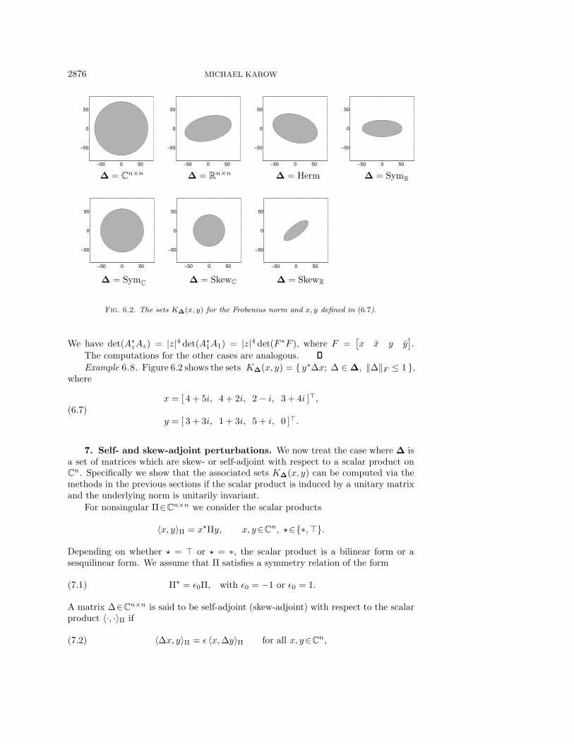
Fig. 6.2. The sets KΔ(x, y) for the Frobenius norm and x, y defined in (6.7).

We have det(A∗zAz) = |z|4 det(A∗

1A1) = |z|4 det(F ∗F ), where F =[x x y y

].

The computations for the other cases are analogous.

Example 6.8. Figure 6.2 shows the sets KΔ(x, y) = { y∗Δx; Δ ∈ Δ, ‖Δ‖F ≤ 1 },where

x = [ 4 + 5i, 4 + 2i, 2− i, 3 + 4i ]�,

y = [ 3 + 3i, 1 + 3i, 5 + i, 0 ]�.(6.7)

7. Self- and skew-adjoint perturbations. We now treat the case where Δ isa set of matrices which are skew- or self-adjoint with respect to a scalar product onCn. Specifically we show that the associated sets KΔ(x, y) can be computed via themethods in the previous sections if the scalar product is induced by a unitary matrixand the underlying norm is unitarily invariant.

For nonsingular Π∈Cn×n we consider the scalar products

〈x, y〉Π = xΠy, x, y∈Cn, �∈{∗,�}.

Depending on whether � = � or � = ∗, the scalar product is a bilinear form or asesquilinear form. We assume that Π satisfies a symmetry relation of the form

Π = ε0Π, with ε0 = −1 or ε0 = 1.(7.1)

A matrix Δ∈Cn×n is said to be self-adjoint (skew-adjoint) with respect to the scalarproduct 〈·, ·〉Π if

〈Δx, y〉Π = ε 〈x,Δy〉Π for all x, y∈Cn,(7.2)


and ε = 1 (ε = −1). The relation (7.2) is easily seen to be equivalent to

ΔΠ = εΠΔ.(7.3)

We denote the sets of self- and skew-adjoint matrices by

struct(Π, �, ε) := { Δ ∈ Cn×n ; ΔΠ = εΠΔ }.

The relation (7.1) implies that (7.3) is equivalent to

(ΠΔ) = ε0 εΠΔ.(7.4)

We thus have the following lemma.Lemma 7.1. Let Π,Δ ∈ Kn×n, where K = R or C. Suppose Π = ε0Π with

ε0 = −1 or ε0 = 1. Then the following equivalences hold:

Δ∈struct(Π, �, ε) ⇔

⎧⎪⎪⎪⎪⎪⎪⎨⎪⎪⎪⎪⎪⎪⎩

ΠΔ∈Herm if ε0ε = 1, � = ∗,ΠΔ∈SymK if ε0ε = 1, � = �,

ΠΔ∈SkewK if ε0ε = −1, � = �,

iΠΔ∈Herm if ε0ε = −1, � = ∗.

In many applications Π is unitary. The most common examples are

Π ∈ {diag(Ik,−In−k), En, Jn},

where

Jn =

[0 In

−In 0

]∈ C

2n×2n, En =

⎡⎢⎣ 1

. ..

1

⎤⎥⎦ ∈ Cn×n.

Proposition 7.2. Suppose Π ∈ Cn×n is unitary and satisfies Π = ε0Π withε0 = −1 or ε0 = 1. Let struct = struct(Π, �, ε). Then, for any unitarily invariantnorm,

Kstruct(x, y) = KΔ(x,Πy),

where

Δ =

⎧⎪⎪⎪⎪⎪⎪⎪⎪⎪⎨⎪⎪⎪⎪⎪⎪⎪⎪⎪⎩

Herm if ε0ε = 1, � = ∗,SymC if ε0ε = 1, � = �,

SymR if ε0ε = 1, � = �, and Π ∈ Rn×n,

SkewC if ε0ε = −1, � = �,

SkewR if ε0ε = −1, � = �, and Π ∈ Rn×n.

(7.5)

Furthermore, Kstruct(x, y) = KHerm(x, iΠy) if ε0ε = −1 and � = ∗.

2878 MICHAEL KAROW

Proof. Using Lemma 7.1 and Π∗Π = In we obtain for the sets in (7.5)

Kstruct(x, y) = { y∗Δx; Δ ∈ struct, ‖Δ‖ ≤ 1 }= { (Πy)∗(ΠΔ)x; ΠΔ ∈ Δ, ‖ΠΔ‖ ≤ 1 }= KΔ(x,Πy).

The proof of the remaining statement is analogous.Example 7.3. In this final example we consider the matrix

A =

⎡⎢⎢⎣α β 1 0−β α 0 10 0 α β0 0 −β α

⎤⎥⎥⎦ , α, β ∈ R, β = 0.(7.6)

Note that A has two Jordan blocks of dimension 2 associated with the eigenvaluesλ = α + iβ, λ = α − iβ. Both eigenvalues are nonderogatory and have algebraicmultiplicity 2. Let x, y ∈ C4 be defined as

x :=1√2[ 1, i, 0, 0 ]�, y :=

1√2[ 1, −i, 1, −i ]∗.

Then

Ax = λx, y∗(A− λ I4)2 = 0, y∗(A− λ I4) = 0, y∗x = 1.

Let y∗ := y∗(A − λ I4) = [ 0, 0, 1,−i ]/√2. According to the discussion in the

introduction we have for the connected component CΔ(A, λ, ε) of the pseudospectrumσΔ(A, ε) that

limε→0

CΔ(A, λ, ε)− λ

ε1/2= K

(2)Δ (x, y),

where K(2)Δ (x, y) = { z; z2 ∈ KΔ(x, y) }. We consider now the case where Δ = R4×4

and where the underlying norm is the Frobenius norm. Then by Theorem 6.5 the setKΔ(x, y) = KR4×4(x, y) equals the ellipse defined in (6.1), where

a =1

2‖x‖2‖y‖2 = 1

2, b =

1

2(x�x) (y�y) = 0.

Since b = 0, the ellipse is a disk of radius√a = 1/

√2. Hence, K

(2)Δ (x, y) is a disk of

radius 2−1/4.Note that the matrix A is Hamiltonian; i.e., A is skew-adjoint with respect to

the skew-Hermitian inner product (v, w) → v∗Jw, J =[

0 I2−I2 0

]. Let HamR =

{Δ ∈ R4×4; Δ�J = −JΔ } denote the set of all real Hamiltonian 4 × 4 matrices.Then, by Lemma 7.1, HamR = {Δ ∈ C4×4; JΔ ∈ SymR } and, by Proposition 7.2,KHamR

(x, y) = KSymR(x, Jy). Hence, if the underlying norm is the Frobenius norm,

then KHamR(x, y) equals the ellipse with the parameters (see Theorem 6.5)

a =1

4(‖x‖2‖Jy‖2 + |x�Jy|2) = 1

4,

b =1

4( (x�x) ((Jy)�(Jy)) + (x∗(Jy))2) =

1

4.


Since a = b, the ellipse degenerates to an interval. Precisely we have KHamR(x, y) =

[−√a+ b,

√a+ b] = [−2−1/2, 2−1/2] and hence K

(2)HamR

(x, y) = [−2−1/4, 2−1/4] ∪i [−2−1/4, 2−1/4].

8. Appendix. We give the proof Lemma 6.7. To this end we need the followingfact.

Proposition 8.1. Let σ1 ≥ σ2 ≥ · · · ≥ σn denote the singular values ofM = AB∗, where A,B ∈ Cn×r. Then σk = 0 for k > r, and σ2

1 , σ22 , . . . , σ

2r are

the eigenvalues of (A∗A)(B∗B). In particular,

r∑k=1

σ2k = tr((A∗A)(B∗B)),

r∏k=1

σ2k = det((A∗A)(B∗B)).

Proof. Since rank(M) ≤ r, we have σk = 0 for k > r. The squares of the singularvalues of M are the eigenvalues of M∗M = XY , where X = B, Y = (A∗A)B∗. As iswell known XY and Y X = (A∗A)(B∗B) have the same nonzero eigenvalues.

Now, let σ1, σ2 denote the largest singular values of the matrix

M = a1b∗1 + a2b

∗2 = [a1 a2] [b1 b2]

∗, a1, a2, b1, b2 ∈ Cn.

Since rank(M) ≤ 2, the other singular values of M are zero. Using Proposition 8.1we obtain for the Frobenius norm and the Schatten-1-norm of M

‖M‖2F = σ21 + σ2

2

= tr

([‖a1‖2 a∗1a2a∗2a1 ‖a2‖2

] [‖b1‖2 b∗1b2b∗2b1 ‖b2‖2

])= ‖a1‖2‖b1‖2 + ‖a2‖2‖b2‖2 + 2�( (a∗1a2) (b∗1b2) ),

‖M‖2(1) = (σ1 + σ2)2

= σ21 + σ2

2 + 2√σ21σ

22

= ‖M‖2F + 2√β,

where

β = det

([‖a1‖2 a∗1a2a∗2a1 ‖a2‖2

] [‖b1‖2 b∗1b2b∗2b1 ‖b2‖2

])= ( ‖a1‖2‖a2‖2 − |a∗1a2|2)(‖b1‖2‖b2‖2 − |b∗1b2|2 ).

Next, we compute the norms of the symmetric and the skew-symmetric parts of M .Let S± = 1

2 (M ±M�). Then S± can be written in the form S± = AB∗±, where

A =[a1 a2 b1 b2

], B± =

1

2

[b1 b2 ±a1 ±a2

].

2880 MICHAEL KAROW

We have

A∗A =

⎡⎢⎢⎢⎢⎣‖a1‖2 a∗1a2 a�1 b1 a�1 b2

a∗2a1 ‖a2‖2 a�2 b1 a�2 b2b�1 a1 b�1 a2 ‖b1‖2 b∗1b2b�2 a1 b�2 a2 b∗2b1 ‖b2‖2

⎤⎥⎥⎥⎥⎦ ,

B∗±B± =

1

4

⎡⎢⎢⎢⎢⎣‖b1‖2 b∗1b2 ± b�1 a1 ± b�1 a2

b∗2b1 ‖b2‖2 ± b�2 a1 ± b�2 a2± a�1 b1 ± a�1 b2 ‖a1‖2 a∗1a2± a�2 b1 ± a�2 b2 a∗2a1 ‖a2‖2

⎤⎥⎥⎥⎥⎦ .

Using Proposition 8.1 we obtain for the Frobenius norm of S±

‖S±‖2F = tr((A∗A)(B∗±B±))

=1

2

( ‖a1‖2‖b1‖2 + ‖a2‖2‖b2‖2 ± |a�1 b1|2 ± |a�2 b2|2)

+ �((a∗1a2) (b

∗1b2) ± (a�1 b2) (a

�2 b1)

).

We now determine the Schatten-1-norm of S−. Since rank(S−) ≤ 4, at most foursingular values of S− are nonzero. Let σ1 ≥ σ2 ≥ σ3 ≥ σ4 denote these singularvalues. Since S− is skew-symmetric, its singular values have even multiplicity [10,section 4.4, Exercise 26]. Thus σ1 = σ2 and σ3 = σ4. This yields

‖S−‖2(1) = (σ1 + σ2 + σ3 + σ4)2

= (2σ1 + 2σ3)2

= 2(2σ21 + 2σ2

3) + 8σ1σ3

= 2‖S−‖2F + 8 (σ21σ

22σ

23σ

24)

1/4

= 2‖S−‖2F + 8 (det[(A∗A)(B∗−B−)] )1/4.

Since 4B∗−B− is unitarily similar to A∗A, we have det(B∗−B−) = 1

256 det(A∗A).

Hence,

‖S−‖2(1) = 2(‖S−‖2F +

√det(A∗A)

).

Acknowledgment. The author thanks the referees for many valuable comments.

REFERENCES

[1] B. Bernhardsson, A. Rantzer, and L. Qiu, Real perturbation values and real quadratic formsin a complex vector space, Linear Algebra Appl., 270 (1998), pp. 131–154.

[2] R. Bhatia, Matrix Analysis, Springer, New York, 1997.[3] S. Bora and V. Mehrmann, Linear perturbation theory for structured matrix pencils arising

in control theory, SIAM J. Matrix Anal., 28 (2006), pp. 148–169.[4] R. Byers and D. Kressner, On the condition of a complex eigenvalue under real perturbations,

BIT, 44 (2004), pp. 209–214.[5] F. Chaitin-Chatelin, A. Harrabi, and A. Ilahi, About Holder condition numbers and the

stratification diagram for defective eigenvalues, Math. Comput. Simulation, 54 (2000),pp. 397–402.


[6] M. Embree and L. N. Trefethen, The Pseudospectra Gateway, http://www.comlab.ox.ac.uk/pseudospectra.

[7] S. Graillat and F. Tisseur, Structured condition numbers and backward errors in scalarproduct spaces, Electron. J. Linear Algebra, 15 (2006), pp. 159–177.

[8] D. Hinrichsen and A. J. Pritchard, Mathematical Systems Theory I, Texts Appl. Math. 48,Springer, Berlin, 2005.

[9] J. Hiriat-Urruty and C. Lemarechal, Fundamentals of Convex Analysis, Springer, Berlin,2001.

[10] R. A. Horn and C. R. Johnson, Matrix Analysis, Cambridge University Press, Cambridge,UK, 1985.

[11] R. A. Horn and C. R. Johnson, Topics in Matrix Analysis, Cambridge University Press,Cambridge, UK, 1991.

[12] M. Karow, Geometry of Spectral Value Sets, Ph.D. thesis, University of Bremen, Bremen,Germany, 2003.

[13] M. Karow, D. Kressner, and F. Tisseur, Structured eigenvalue condition numbers, SIAMJ. Matrix Anal. Appl., 28 (2006), pp. 1052–1068.

[14] T. Kato, Perturbation Theory for Linear Operators, Springer, Berlin, 1980.[15] D. Kressner, M. J. Pelaez, and J. Moro, Structured Holder condition numbers for multiple

eigenvalues, SIAM J. Matrix Anal. Appl., 31 (2009), pp. 175–201.[16] J. Moro, J. V. Burke, and M. L. Overton, On the Lidskii–Vishik–Lyusternik perturbation

theory for eigenvalues of matrices with arbitrary Jordan structure, SIAM J. Matrix Anal.Appl., 18 (1997), pp. 793–817.

[17] S. Noschese and L. Pasquini, Eigenvalue condition numbers: Zero-structured versus tradi-tional, J. Comput. Appl. Math., 185 (2006), pp. 174–189.

[18] S. Noschese and L. Pasquini, Eigenvalue patterned condition numbers: Toeplitz and Hankelcases, J. Comput. Appl. Math., 206 (2007), pp. 615–624.

[19] J. R. Rice, A theory of condition, SIAM J. Numer. Anal., 3 (1966), pp. 287–310.[20] S. M. Rump, Eigenvalues, pseudospectrum and structured perturbations, Linear Algebra Appl.,

413 (2006), pp. 567–593.[21] S. M. Rump and H. Sekigawa, The ratio between the Toeplitz and the unstructured condition

number, in Numerical Methods for Structured Matrices and Applications, Oper. TheoryAdv. Appl. 199, Birkhauser, Basel, 2010, pp. 397–419.

[22] G. W. Stewart and J. Sun, Matrix Perturbation Theory, Academic Press, San Diego, 1990.[23] F. Tisseur, A chart of backward errors for singly and doubly structured eigenvalue problems,

SIAM J. Matrix Anal. Appl., 24 (2003), pp. 877–897.[24] L. N. Trefethen and M. Embree, Spectra and Pseudospectra: The Behavior of Nonnormal

Matrices and Operators, Princeton University Press, Princeton, NJ, 2005.

STRUCTURED PSEUDOSPECTRA AND THE - TU Berlin

Documents

Transcript of STRUCTURED PSEUDOSPECTRA AND THE - TU Berlin