arX

iv:1

202.

1186

v2 [

cs.D

C]

5 A

pr 2

012

Stone Age Distributed Computing

Yuval Emek Jasmin Smula Roger Wattenhofer

Computer Engineering and Networks Laboratory (TIK)

ETH Zurich, Switzerland

Abstract

The traditional models of distributed computing focus mainly on networks of computer-like

devices that can exchange large messages with their neighbors and perform arbitrary local com-

putations. Recently, there is a trend to apply distributed computing methods to networks of

sub-microprocessor devices, e.g., biological cellular networks or networks of nano-devices. How-

ever, the suitability of the traditional distributed computing models to these types of networks

is questionable: do tiny bio/nano nodes “compute” and/or “communicate” essentially the same

as a computer? In this paper, we introduce a new model that depicts a network of randomized

finite state machines operating in an asynchronous environment. Although the computation

and communication capabilities of each individual device in the new model are, by design, much

weaker than those of a computer, we show that some of the most important and extensively

studied distributed computing problems can still be solved efficiently.

1 Introduction

Networks are at the core of many scientific areas, be it social sciences (where networks for instance

model human relations), logistics (e.g. traffic), or electrical engineering (e.g. circuits). Distributed

computing is the area that studies the power and limitations of distributed algorithms and com-

putation in networks. Due to the major role that the Internet plays today, models targeted at

understanding the fundamental properties of networks focus mainly on “Internet-capable” devices.

The standard model in distributed computing is the so called message passing model, where nodes

may exchange large messages with their neighbors, and perform arbitrary local computations.

Some networks though, are not truthfully represented by the classical message passing model.

For example, wireless networks such as ad hoc or sensor networks, whose research has blossomed in

the last decade, require some adaptations of the message passing model so that it meets the limited

capabilities of the underlying wireless devices more precisely. More recently, there is a trend to

apply distributed computing methods, and in particular, the message passing model, to networks

of sub-microprocessor devices, for instance networks of biological cells or nano-scale mechanical

devices. However, the suitability of the message passing model to these types of networks is far

from being certain: do tiny bio/nano nodes “compute” and/or “communicate” essentially the same

as a computer? Since such nodes will be fundamentally more limited than silicon-based devices, we

believe that there is a need for a network model, where nodes are by design below the computation

and communication capabilities of Turing machines.

Networked Finite State Machines. In this paper, we take a radically different approach:

Instead of imposing additional restrictions on the existing models for networks of computer-like

devices, we introduce an entirely new model, referred to as networked finite state machines (nFSM),

that depicts a network of randomized finite state machines progressing in asynchronous steps (refer

to Section 2 for a formal description). Under the nFSM model, nodes communicate by transmitting

messages belonging to some finite communication alphabet Σ such that a message σ ∈ Σ transmitted

by node u is delivered to its neighbors (the same σ to all neighbors) in an asynchronous fashion;

each neighbor v of u has a port corresponding to u in which the last message delivered from u is

stored.

The access of node v to its ports is limited: each state q in the state set Q of the FSM is

associated with some query letter σ = σ(q) ∈ Σ; if node v resides in state q at some step of the

execution, then the next state and the message transmitted by v at this step are determined by q and

by the number ♯(σ) of occurrences of σ in v’s ports. The crux of the model is that ♯(σ) is calculated

according to the one-two-many1 principle: the node can only count up to some predetermined

1 The one-two-many theory states that some small isolated cultures (e.g., the Piraha tribe of the Amazon [20])

did not develop a counting system that goes beyond 2. This is reflected in their languages that include words for

“1”, “2”, and “many” that stands for any number larger than 2.

1

bounding parameter b ∈ Z>0 and any value of ♯(σ) larger than b cannot be distinguished from b.

In particular, the nFSM model satisfies the following model requirements, that we believe, make

it more applicable to the study of networks consisting of weaker devices such as those mentioned

above.

(M1) The model is applicable to arbitrary network topologies.

(M2) All nodes run the same protocol executed by a (randomized) FSM.

(M3) The network operates within an asynchronous environment, with node activation patterns

independent of message delivery patterns.

(M4) All features of the FSM (specifically, the state set Q, message alphabet Σ, and bounding

parameter b) are of constant size independent of any parameter of the network (including the degree

of the node executing the FSM).

The last requirement is perhaps the most interesting one as it implies that a node cannot perform

any calculation that involves numbers beyond some predetermined constant. This comes in contrast

to many distributed algorithms operating under the message passing model that strongly rely on

the ability of a node to perform such calculations (e.g., count up to some parameter of the network

or a function thereof).

Results. Our investigation of the new model begins by implementing an nFSM synchronizer that

practically allows the algorithm designer to assume a synchronous environment (Section 3). Then,

we show that the computational power of a network operating under the nFSM model is essentially

equivalent to that of a randomized Turing machine with linear space bound (cf. linear bounded

automaton). In comparison, the computational power of a network operating under the message

passing model is trivially equivalent to that of a (general) Turing machine, therefore there exist

distributed problems that can be solved under the message passing model in constant time but

cannot be solved under the nFSM model at all (Section 6).

Nevertheless, we show that arguably the most important and extensively studied problems in

distributed computing admit efficient — namely, with run-time polylogarithmic in the number of

nodes — algorithms operating under the nFSM model. Specifically, we develop such algorithms

for computing a maximal independent set (MIS) in arbitrary graphs (Section 4) and for 3-coloring

of (undirected) trees (Section 5). We also develop an efficient algorithm that computes a maximal

matching in arbitrary graphs, but this requires a small unavoidable modification of the nFSM model

that goes beyond the scope of the current version of the paper.

Related Work. As mentioned above, the message passing model is the gold standard when it

comes to understanding distributed algorithms. Several variants exist for this model, differing

mainly in the bounds imposed on the message size and the level of synchronization. Perhaps

the most popular message passing variants are the fully synchronous local and congest models

[26, 31, 36], assuming that in each round, a node can send messages to its neighbors (different

2

messages to different neighbors), receive and interpret the messages sent to it from its neighbors,

and perform an arbitrary local computation2 determining, in particular, the messages sent in the

next round. The difference between the two variants is cast in the size of the communicated

messages: the local model does not impose any restrictions on the message size, hence it can be

used for the purpose of establishing general lower bounds, whereas the congest model is more

information-theoretic, with a (typically logarithmic) bound on the message size. Indeed, most

theoretical literature dealing with distributed algorithms relies on one of these two models.

As the congest model still allows for sending different messages to different neighbors in each

round, it was too powerful for many settings. Instead, with the proliferation of wireless networks,

new more restrictive message passing models appeared such as the radio network model [13]. In

radio networks, nodes still operate in synchronous rounds, where in each round a node may choose

to transmit a message or stay silent. A transmitted message is received by all neighbors in the

network if the neighbors do not experience interference by concurrently transmitting nodes in their

own neighborhood. There are several variants, e.g. whether nodes have collision detection, or not.

Since the radio network model is still too powerful for some wireless settings, more restrictive

models were suggested. One such example is the beeping model [17, 16], where in each round a

node can either beep or stay silent, and a silent node can only distinguish between the case in

which no node in its neighborhood beeps and the case in which at least one node beeps. Efficient

algorithms and lower bounds for the MIS problem under the beeping model were developed by Afek

et al. [2, 1]. Note that the beeping model resembles our nFSM model in the sense that the “beeping

rule” can be viewed as counting under the one-two-many principle with bounding parameter b = 1.

However, it is much stronger in other perspectives: (i) the beeping model assumes synchronous

communication and does not seem to have a natural asynchronous variant, thus it does not satisfy

requirement (M3); and (ii) the local computation is performed by a Turing machine whose memory

is allowed to grow with the network (this is crucial for the algorithms of Afek et al. [2, 1]), thus it

does not satisfy requirements (M2) and (M4).

Our nFSM model is a generalization of the extensively studied cellular automaton model [30,

18, 38] that captures a network of FSMs, arranged in a grid topology (some other highly regular

topologies were also considered), where the transition of each node depends on its current state

and the states of its neighbors. Still, the nFSM model differs from the cellular automaton model in

many aspects; in particular, the latter model is not applicable for non-regular network topologies,

in contrast to requirement (M1), and to the most part, it also does not support asynchronous

environments (at least not as asynchrony is grasped in the current paper), in contrast to requirement

(M3).

Another model that resembles the nFSM model is that of communicating automata [12]. This

2 It is important to point out that even though the local and congest models allow for arbitrary local computations,

the existing literature hardly ever assumes anything that cannot be computed in time polynomial in the size of the

information received thus far; the rare exceptions are typically clearly mentioned in the text.

3

model also assumes that each node in the network operates a FSM in an asynchronous manner,

however the steps of the FSMs are message driven: for each state q of node v and for each message

m that node v may receive from an adjacent node u while residing in state q, the transition

function of v should have an entry characterized by the 3-tuple (q, u,m) that determines its next

move. As such, different nodes would typically operate different FSMs, hence the model does

not satisfy requirement (M2), and more importantly, the size of the FSM operated by node v

inherently depends on the degree of v, hence it does not satisfy requirement (M4). Moreover, the

node activation pattern is driven by the incoming messages, so it also does not satisfy requirement

(M3).

Applicability to Biological Cellular Networks. Regardless of the theoretical interest in im-

plementing efficient algorithms using weaker assumptions, we believe that our new model and

results should be appealing to anyone interested in understanding the computational aspects of

biological cellular networks. A basic dogma in biology (see, e.g., [33]) states that all cells commu-

nicate and that they do so by emitting special kinds of proteins (e.g., cytokines and chemokines

in the immune system) that can be recognized by designated receptors, thus enabling neighboring

cells to distinguish between different concentration levels of these proteins, which, after a signaling

cascade, leads to different gene expression.

Translated to the language of the nFSM model, the emitted proteins correspond to the letters

of the communication alphabet, where the actual emission corresponds to transmitting a letter, and

the ability of a cell to distinguish between different concentration levels of these proteins corresponds

to the manner in which the nodes in our model interpret the content of their ports. Using an FSM

as the underlying computational model of each node seems to be the right choice especially in the

biological setting as demonstrated by Benenson et al. [11] who showed that essentially any FSM

can be implemented by enzymes found in cells’ nuclei. One may wonder if the specific problems

studied in the current paper have any relevance to biological cellular networks. Indeed, Afek et

al. [2] discovered that a biological process that occurs during the development of the nervous system

of a fly is in fact equivalent to solving the MIS problem.

2 Model

Throughout, we assume a network represented by a finite undirected graph G = (V,E). Under the

networked finite state machines (nFSM) model, each node v ∈ V runs a protocol depicted by the

8-tuple

Π = 〈Q,QI , QO,Σ, σ0, b, λ, δ〉 ,where

• Q is a finite set of states;

4

• QI ⊆ Q is the subset of input states;

• QO ⊆ Q is the subset of output states;

• Σ is a finite communication alphabet ;

• σ0 ∈ Σ is the initial letter ;

• b ∈ Z>0 is a bounding parameter ; let B = 0, 1, . . . , b− 1,≥b be a set of b+1 distinguishable

symbols;

• λ : Q→ Σ assigns a query letter σ ∈ Σ to every state q ∈ Q; and

• δ : Q×B → 2Q×(Σ∪ε) is the transition function.

It is important to point out that protocol Π is oblivious to the graph G. In fact, the number of

states in Q, the size of the alphabet Σ, and the bounding parameter b are all assumed to be universal

constants, independent of any parameter of the graph G. In particular, the protocol executed by

node v ∈ V does not depend on the degree of v in G. We now turn to describe the semantics of

the nFSM model.

Communication. Node v communicates with its adjacent nodes in G by transmitting messages.

A transmitted message consists of a single letter σ ∈ Σ and it is assumed that this letter is delivered

to all neighbors u of v. Each neighbor u has a port ψu(v) (a different port for every adjacent node

v) in which the last message σ received from v is stored. At the beginning of the execution, all

ports store the initial letter σ0. It will be convenient to consider the case in which v does not

transmit any message (and hence does not affect the corresponding ports of the adjacent nodes) as

a transmission of the special empty symbol ε.

Execution. The execution of node v progresses in discrete steps indexed by the positive integers.

At each step t ∈ Z>0, v resides in some state q ∈ Q. Let λ(q) = σ ∈ Σ be the query letter that λ

assigns to state q and let ♯(σ) be the number of occurrences of σ in v’s ports in step t. Then, the

pair (q′, σ′) of state q′ ∈ Q in which v resides in step t+1 and message σ′ ∈ Σ∪ε transmitted by

v in step t (recall that ε indicates that no message is transmitted) is chosen uniformly at random

(and independently of all other random choices) among the pairs in

δ (q, fb (♯(σ))) ⊆ Q× (Σ ∪ ε) ,

where fb : Z≥0 → B is defined as

fb(x) =

x if 0 ≤ x ≤ b− 1 ;≥b otherwise .

Informally, this can be thought of as if v queries its ports for occurrences of σ and “observes” the

exact value of ♯(σ) as long as it is smaller than the bounding parameter b; otherwise, v merely

“observes” that ♯(σ) ≥ b which is indicated by the symbol ≥b.

5

Input and Output. Initially (in step 1), each node resides in some of the input states in QI .

The choice of the initial state of node v ∈ V reflects the input passed to v at the beginning of the

execution. This allows our model to cope with distributed problems in which different nodes get

different input symbols. When dealing with problems in which the nodes do not get any initial

input (such as the graph theoretic problems addressed in this paper), we shall assume that QI

contains a single initial state.

We say that the (global) execution of the protocol is in an output configuration if all nodes

reside in output states of QO. If this is the case, then the output of node v ∈ V is determined by

the output state q ∈ QO in which v resides.

Asynchrony. The nodes are assumed to operate in an asynchronous environment. This asyn-

chrony has two facets: First, for the sake of convenience, we assume that the actual application

of the transition function in each step t ∈ Z>0 of node v ∈ V is instantaneous (namely, lasts zero

time) and occurs at the end of the step;3 the length of step t of node v, denoted Lv,t, is defined as

the time difference between the application of the transition function in step t− 1 and that of step

t. It is assumed that Lv,t is finite, but apart from that, we do not make any further assumptions

on this length, that is, the step length Lv,t is determined by the adversary independently of all

other step lengths Lv′,t′ . In particular, we do not assume any synchronization between the steps of

different nodes whatsoever.

Another facet of the asynchronous environment is that a message transmitted by node v in

step t (if such a message is transmitted) is assumed to reach the port ψu(v) of an adjacent node

u after a finite time delay, denoted Dv,t,u. We assume that if v transmits message σ1 ∈ Σ in step

t1 and message σ2 ∈ Σ in step t2 > t1, then σ1 reaches u before σ2 does. Apart from this “FIFO”

assumption, we do not make any other assumptions on the delays Dv,t,u. In particular, this means

that under certain circumstances, the adversary may overwrite message σ1 with message σ2 in port

ψu(v) of u so that u will never “know” that message σ1 was transmitted.4

Consequently, a policy of the adversary is captured by: (1) the length Lv,t of step t of node v

for every v ∈ V and t ∈ Z>0; and (2) the delay Dv,t,u of the delivery of the transmission of node

v in step t to an adjacent node u for every v ∈ V , t ∈ Z>0, and u ∈ N (v).5 Assuming that the

adversary is oblivious to the random coin tosses of the nodes, an adversarial policy is depicted by

infinite sequences of Lv,t and Dv,t,u parameters.

3 This assumption can be lifted at the cost of a more complicated definition of the adversarial policy described

soon.4 Often, much stronger assumptions are made in the literature. For example, a common assumption for asyn-

chronous environments is that the port of node u corresponding to the adjacent node v is implemented by a buffer

so that messages cannot be “lost”. We do not make any such assumption for our nFSM model.5 We use the standard notation N (v) for the neighborhood of node v in G, namely, the subset of nodes adjacent

to v.

6

For further information on asynchronous environments, we point the reader to one of the stan-

dard textbooks [31, 28].

Correctness and Run-Time Measures. A protocol Π for problem P is said to be correct under

the nFSM model if for every instance of P and for every adversarial policy, Π reaches an output

configuration within finite time with probability 1, and for every output configuration reached by Π

with positive probability, the output of the nodes is a valid solution to P . Given a correct protocol

Π, the complexity measure that interests us in the current paper is the run-time of Π defined as

follows.

Consider some instance I of problem P . Given an adversarial policy A and a sequence (actually

an n-tuple of sequences) R of random coin tosses that lead to an output configuration within finite

time, the run-time TΠ(I,A,R) of Π on I with respect to A and R is defined as the (possibly

fractional) number of time units6 that pass from the beginning of the execution until the first time

the protocol reaches an output configuration, where a time unit is defined to be the maximum

among all step length parameters Lv,t and delivery delay parameters Dv,t,u appearing in A before

the output configuration is reached. Let TΠ(I,A) denote the random variable that depicts the

run-time of Π on I with respect to A. Following the standard procedure in this regard, we say that

the run-time of a correct protocol Π for problem P is f(n) if for every n-node instance I of P and

for every adversarial policy A, it holds that TΠ(I,A) is at most f(n) in expectation and with high

probability. The protocol is said to be efficient if its run-time is polylogarithmic in the size of the

network (cf. [26]).

3 Convenient Transformations

In this section, we show that the nFSM protocol designer may, in fact, assume a slightly more

“user-friendly” environment than the one described in Section 2. This is based on the design of

black-box compilers transforming a protocol that makes strong assumptions on the environment

into one that does not make any such assumptions. Specifically, the assumptions that can be lifted

that way are synchrony (Section 3.1), and multiple-letter queries (Section 3.2).

3.1 Implementing a Synchronizer

As described in Section 2, the nFSM model assumes an asynchronous environment. Nevertheless,

it will be convenient to extend the nFSM model to synchronous environments. One natural such

extension augments the model described in Section 2 with the following two synchronization prop-

6 Note that time units are defined solely for the purpose of the analysis. Under an asynchronous environment, the

nodes have no notion of time and in particular, they cannot measure a single time unit.

7

erties for every two adjacent nodes u, v ∈ V and for every t ∈ Z>0:

(S1) when node u is in step t, node v is in step t− 1, t, or t+ 1; and

(S2) at the end of step t+ 1 of u, port ψu(v) stores the message transmitted by v in step t of v’s

execution (or the last message transmitted by v prior to step t if v does not transmit any message

in step t).

An environment in which properties (S1) and (S2) are guaranteed to hold is called a locally syn-

chronous environment. Local-only communication can never achieve global synchrony, however,

research in the message passing model has shown that local synchrony is often sufficient to provide

efficient algorithms [4, 6, 5]. To distinguish a protocol assumed to operate in a locally synchronous

environment from those making no such assumptions, we shall often refer to the execution steps of

the former as rounds (cf. fully synchronized protocols). Our goal in this section is to establish the

following theorem.

Theorem 3.1. Every nFSM protocol Π = 〈Q,QI , QO,Σ, σ0, b, λ, δ〉 designed to operate in a locally

synchronous environment can be simulated in an asynchronous environment by a protocol Π at the

cost of a constant multiplicative run-time overhead.

The procedure in charge of the simulation promised in Theorem 3.1 is referred to as a synchro-

nizer [4]. The remainder of Section 3.1 is dedicated to the design (and analysis) of a synchronizer

for the nFSM model.

Overview. Round t ∈ Z>0 of node v ∈ V under Π is simulated by O(1) contiguous steps under

Π; the collection of these steps is referred to as v’s simulation phase of round t. Protocol Π is

designed so that v maintains the value of t mod 3, referred to as the trit (trinary digit) of round t,

which is also encoded in the message transmitted by v at the end of round t.7 The main principle

behind our synchronizer is that node v will not move to the simulation phase of round t+ 1 while

its ports still contain messages sent in a round whose trit is t− 1 mod 3.

Under Π, the decisions made by node v at round t should be based on the messages transmitted

by all neighbors u of v at round t− 1. However, during v’s simulation phase of round t, port ψv(u)

may contain messages transmitted at round t− 1 or at round t under Π. The latter case is prob-

lematic since the message transmitted by u in the simulation phase of round t− 1 is overwritten by

that transmitted in the simulation phase of round t. To avoid this obstacle, a message transmitted

by node u under Π at the end of the simulation phase of round t also encodes the message that u

transmitted under Π at round t− 1.

So, if v resides in a state whose query letter is σ ∈ Σ in round t under Π, then under Π, v should

query for all Σ-letters encoding a transmission of σ at round t − 1. Since there are several such

letters, a carefully designed feature should be used so that Π accounts for their combined number.

7 Note that maintaining the value of t mod 2 is insufficient for the sake of reaching synchronization.

8

Protocol Π. Let

Π =⟨Q, QI , QO, Σ, σ0, b, λ, δ

⟩.

Consider node v ∈ V and round t ∈ Z>0. As the name implies, node v’s simulation phase of round

t under Π, denoted φv(t), corresponds to round t of Π. Protocol Π is designed so that at every

step in φv(t) other than the last one, v does not transmit any message (indicated by transmitting

ε), and at the last step of the simulation phase, v always transmits some message σ ∈ Σ, denoted

Mv(t).

The alphabet Σ is defined to be

Σ′ = (Σ ∪ ε) × (Σ ∪ ε) × 0, 1, 2 .

The semantics of the message Mv(t) = (σ, σ′, j) sent by node v at the last step of the simulation

phase φv(t) is that: v transmits σ ∈ Σ ∪ ε at round t − 1 under Π; v transmits σ′ ∈ Σ ∪ ε atround t under Π; and j = t mod 3. Following that logic, we set σ0 = (ε, σ0, 0).

The state set Q of Π is defined to be

Q =

⋃

q∈Q

(Pq ∪ Sq)

× 0, 1, 2 ,

where Pq × j and Sq × j, q ∈ Q, j ∈ 0, 1, 2, are referred to as the pausing and simulating

features, respectively, whose role will be clarified soon. Suppose that v resides in state q ∈ Q in

step t under Π and that j = t mod 3. Then, throughout φv(t), node v resides in some state in

(Pq ∪ Sq) × j. In particular, in the first steps of the simulation phase, v resides in states of the

pausing feature Pq ×j, and then at some stage it switches to the simulating feature Sq×j andremains in its states until the end of the simulation phase.

The Pausing Feature. For the simulation phase of round t, we denote the letters in (Σ∪ε)×(Σ ∪ ε) × j − 2 as dirty and the letters in (Σ ∪ ε) × (Σ ∪ ε) × j − 1, j as clean.8 The

purpose of the pausing feature Pq×j is to pause the execution of v until its ports do not contain

any dirty letter. This is carried out by including in Pq × j a state pσ,σ′ for every σ, σ′ ∈ Σ ∪ ε;the query letter of pσ,σ′ is (the dirty letter) λ(pσ,σ′) = (σ, σ′, j − 2) and the transition function δ is

designed so that v moves to the next (according to some fixed order) state in the feature Pq × jif and only if there are no ports storing the query letter.

We argue that the pausing feature guarantees synchronization property (S1). For the sake of

the analysis, it is convenient to assume the existence of a fully synchronous simulation phase of

a virtual round 0; upon completion of this simulation phase (at the beginning of the execution),

every node v ∈ V transmits the message Mv(0) = σ0. We are now ready to establish the following

lemma.8 Throughout this section, arithmetic involving the parameter j is done modulo 3.

9

Lemma 3.2. For every t ∈ Z>0, v ∈ V , and u ∈ N (v), when v completes the pausing feature of

φv(t), port ψv(u) stores either Mu(t− 1) or Mu(t).

Proof. By induction on t. The base case of round t = 0 holds by our assumption that φv(0)

and φu(0) are fully synchronous. Assume by induction that the assertion holds for round t − 1.

Applying the inductive hypothesis to both u and v, we conclude that (1) when v completes the

pausing feature of φv(t − 1), port ψv(u) stores either Mu(t − 2) or Mu(t − 1); and (2) when u

completes the pausing feature of φu(t− 1), port ψu(v) stores either Mv(t− 2) or Mv(t− 1).

Let τu and τv denote the times at which u and v complete the pausing feature of φu(t) and

φv(t), respectively. Since v cannot complete the pausing feature of φv(t) while Mu(t − 2) is still

stored in ψv(u), it follows that at time τv, port ψv(u) stores the message Mu(t′) for some t′ ≥ t− 1.

Our goal in the remainder of this proof is to show that t′ ≤ t. If τv < τu, then t′ must be exactly

t− 1, which concludes the inductive step for that case.

So, assume that τv > τu and suppose by contradiction that t′ ≥ t + 1. Using the same line of

arguments as in the previous paragraph, we conclude that at time τu, port ψu(v) stores the message

Mv(t− 1). Node u cannot complete the pausing feature of φu(t+ 1) while Mv(t− 1) is still stored

in ψu(v), hence v must have transmitted Mv(t) before u completed the pausing feature of φu(t+1).

But this means that v completed the pausing feature of φv(t) before u could have transmitted

Mu(t+ 1), in contradiction to the assumption that ψv(u) stores Mu(t′) for some t′ ≥ t+ 1 at time

τv. The assertion follows.

Consider two adjacent nodes u, v ∈ V . If node u is at round t− 1 when an adjacent node v is

at round t + 1, then v completed the pausing feature of φv(t) before u transmitted Mu(t − 1), in

contradiction to Lemma 3.2. Therefore, our synchronizer satisfies synchronization property (S1).

Furthermore, a similar argument shows that between the time v completed the pausing feature of

φv(t) and the time v completed the simulation phase φv(t) itself, the content of ψv(u) may change

from Mu(t− 1) to Mu(t) (if it was not already Mu(t)), but it will not store Mu(t′) for any t′ > t.

This fact is crucial for the implementation of the simulation feature.

The Simulation Feature. Upon completion of the pausing feature Pq × j, v moves on to the

simulation feature Sq × j. The purpose of this feature is to perform the actual simulation of

round t in v, namely, to determine the state (of Q) dominating the simulation phase of the next

round and the message transmitted when moving from the simulation phase of the current round

to that of the next round.

To see how this works out, suppose that λ(q) = σ ∈ Σ. We would have wanted node v to

count (up to the bounding parameter b) the number of occurrences of Σ-letters in its ports that

correspond to the transmission of σ at round t− 1 under Π, that is, the number of occurrences of

10

letters in Γt−1 ∪ Γt, where

Γt−1 =(σ′, σ, j − 1

)| σ′ ∈ Σ ∪ ε

and Γt =

(σ, σ′, j

)| σ′ ∈ Σ ∪ ε

.

More formally, the application of the transition function δ at the end of the simulation phase φv(t)

should be based on fb(∑

γ∈Γt−1∪Γt♯(γ)), where ♯(γ) stands for the number of occurrences of the

letter γ in the ports of v at the end of φv(t).

Identifying the integer b with the symbol ≥b, we observe that the function fb : Z≥0 → B satisfies

fb(x+ y) = min fb(x) + fb(y), b

for every x, y ∈ Z≥0. A natural attempt to compute fb(∑

γ∈Γt−1∪Γt♯(γ)) would include in the

feature Sq×j a state sγ,i for every letter γ ∈ Γt−1∪Γt and integer i ∈ 0, . . . , b; the query letter

of sγ,i would be λ(sγ) = γ and the transition function δ would be designed so that v moves from sγ,i

to sγ′,i′ , where γ′ follows γ in some fixed order of the letters in Γt−1∪Γt and i

′ = mini+fb(♯(γ)), b.

However, care must be taken with this approach since ♯(γ) may decrease (respectively, increase)

during φv(t) for γ ∈ Γt−1 (resp., for γ ∈ Γt) due to new incoming messages. To avoid this obstacle,

we design the feature Sq × j so that first, it computes ϕ1 ← fb(∑

γ∈Γt−1♯(γ)); next, it computes

ϕ2 ← fb(∑

γ∈Γt♯(γ)); and finally, it computes “again” ϕ3 ← fb(

∑γ∈Γt−1

♯(γ)). If φ1 = φ3, then the

current simulation phase is over and δ is applied, simulating δ(q, fb(φ1+φ2)); otherwise, the feature

Sq × j is invoked from scratch. Since the value of fb(∑

γ∈Γt−1♯(γ)) cannot increase during the

simulation phase, and since φ1 ≤ b, the feature Sq ×j is invoked at most b times throughout the

execution of the simulation phase. By induction on t, we conclude that our synchronizer satisfies

synchronization property (S2), which concludes the correctness proof of the simulation.

Accounting. It remains to show that all ingredients of protocol Π are of constant size and that the

run-time of protocol Π incurs at most a constant multiplicative overhead on top of that of protocol

Π. The former claim is established by following our synchronizer construction, observing that

|Σ| = O(|Σ|2

)and |Q| = O

(|Q| · (|Σ|2 + |Σ| · b)

)(recall that the bounding parameter b remains

unchanged). For the latter claim, we need the following definition: given some node subset U ∈ Vand round t ∈ Z>0, let τ(U, t) denote the first time at which u completed simulation phase φu(t)

for all nodes u ∈ U . The following proposition can now be established.

Proposition 3.3. For every node v ∈ V and round t ∈ Z>0, the time difference τ(v, t + 1) −τ(N (v) ∪ v, t) is (up)bounded by a constant.

Proof. Since each transmitted message has a delay of at most 1 unit of time, it follows that by

time τ(N (v) ∪ v, t) + 1, message Mu(t) must reach ψv(u) for all u ∈ N (v). The pausing and

simulation features of φv(t+1) are then completed within O(|Σ|2) and O(|Σ| · b) steps, respectively.The assertion follows as each step lasts for at most 1 unit of time.

11

Employing Proposition 3.3, we conclude by induction on t that τ(V, t) = O(t) for every t ∈ Z>0,

hence if the execution of protocol Π requires T rounds, then the execution of protocol Π is completed

within O(T ) time units. Theorem 3.1 follows.

3.2 Multiple-Letter Queries

Recall that according to the model presented in Section 2, each state q ∈ Q is associated with a

query letter λ(q) and the application of the transition function when node v resides in state q is

determined by fb(♯(σ)), where ♯(σ) is the number of occurrences of the letter σ in the ports of

v. From the perspective of the protocol designer, it is often more convenient to assume that the

node queries on all letters simultaneously, namely, that the application of the transition function

is determined by the vector 〈fb(♯(σ))〉σ∈Σ.

Now that we may assume a synchronous environment, this stronger multiple-letter queries

assumption can easily be supported. Indeed, at the cost of increasing the number of states and the

run-time by constant factors, one can subdivide each round into |Σ| subrounds, dedicating each

subround to a different letter in Σ, so that at the end of the round, the state of v reflects fb(♯(σ))

for every σ ∈ Σ.

Theorem 3.4. Every nFSM protocol with multiple-letter queries can be simulated by an nFSM

protocol with single-letter queries at the cost of a constant multiplicative run-time overhead.

4 Maximal Independent Set

Given a graph G = (V,E), the maximal independent set (MIS) problem asks for a node subset

U ⊆ V which is independent in the sense that (U × U) ∩ E = ∅, and maximal in the sense that

U ′ ⊆ V is not independent for every U ′ ⊃ U . Distributed MIS algorithms with logarithmic run-time

operating in the message passing model were presented by Luby [27] and independently, by Alon

et al. [3];9 Luby’s algorithm has since become a specimen of distributed algorithms; in the last 25

years, researchers have tried to improve it, if only e.g., with an improved bit complexity [29], on

special graph classes [34, 25], or in a weaker communication model [1]. An Ω(√log n)-lower bound

on the run-time of any distributed MIS algorithm operating in the message passing model was

established by Kuhn et al. [23]. Our goal in this section is to design an nFSM protocol for the MIS

problem with run-time O(log2 n).

Outline of the Key Technical Ideas. Our protocol is inspired by the existing message passing

MIS algorithms. Common to all these algorithms is that they are based on the concept of grouping

9 The focus of [27] and [3] was actually on the PRAM model, but their algorithms can be adapted to the message

passing model.

12

consecutive rounds into phases, where in each phase, nodes compete against their neighbors over

the right to join the MIS. Existing implementations of such competitions require at least one of

the following three capabilities: (1) performing calculations that involve super-constant numbers;

(2) communicating with each neighbor independently; or (3) sending messages of super-constant

size, specifically, of size c log n for some constant c > 0. The first two capabilities are clearly out of

the question for an nFSM protocol. The third one is also not supported by the nFSM model, but

perhaps one can divide a message with a logarithmic number of bits over logarithmic many rounds,

sending 1 (or O(1)) bits per round (cf. Algorithm B in [29])?

This naive attempt results in phases of length c log n. However, no FSM can count the rounds

in a c log n long phase — a task essential for deciding if the current phase is over and the next one

should begin. Furthermore, to guarantee fair competition, the phases must be aligned across the

network, thus ruling out the possibility to start node v’s phase i before phase i − 1 of some node

u ∈ N (v) is finished. In fact, an efficient algorithm that requires ω(1) long aligned phases cannot

be implemented under the nFSM model. So, how can we decide if node v joins the MIS using

constant size messages without the ability to maintain long aligned phases?

This issue is resolved by relaxing the requirements that the phases are aligned and of a pre-

determined length, introducing a feature referred to as a tournament. Our tournaments are only

“softly” aligned and their lengths are determined probabilistically, in a manner that can be main-

tained under the nFSM model. Nevertheless, they enable a fair competition between neighboring

nodes, as desired.

The Protocol. Employing Theorems 3.1 and 3.4, we assume a locally synchronous en-

vironment and use multiple-letter queries. The state set of the protocol is Q =

WIN, LOSE, DOWN1, DOWN2, UP0, UP1, UP2, with QI = DOWN1 (the initial state of all nodes) and

QO = WIN, LOSE, where WIN (respectively, LOSE) indicates membership (resp., non-membership)

in the MIS output by the protocol. The states in QA = Q − QO are called the active states and

a node in an active state is referred to as an active node. We take the communication alphabet

Σ to be identical to the state set Q, where the letter transmissions are designed so that node v

transmits letter q whenever it moves to state q from some state q′ 6= q; no letter is transmitted in

a round at which v remains in the same state. Letter DOWN1 is the initial letter stored in all ports

at the beginning of the execution. The bounding parameter is set to b = 1.

A schematic description of the transition function is provided in Figure 1; its logic is as follows.

Each state q ∈ QA has a subset D(q) ⊆ QA of delaying states: node v remains in the current

state q as long as (at least) one of its neighbors is in some state in D(q). This is implemented by

querying on the letters (corresponding to the states) in D(q), staying in state q as long as at least

one of these letters is found in the ports. Specifically, state DOWN1 is delayed by state DOWN2, which

is delayed by all three UP states. State UPj , j = 0, 1, 2, is delayed by state UPj−1 mod 3, where state

13

D1 U0

U1

U2

D2 LWu0 + u1 = 0

u0 + u1 ≥ 1

u1+u2

= 0 u1 + u

2 ≥ 1

u0 + u

2 = 0 u0+u2 ≥

1

w = 0

w ≥ 1

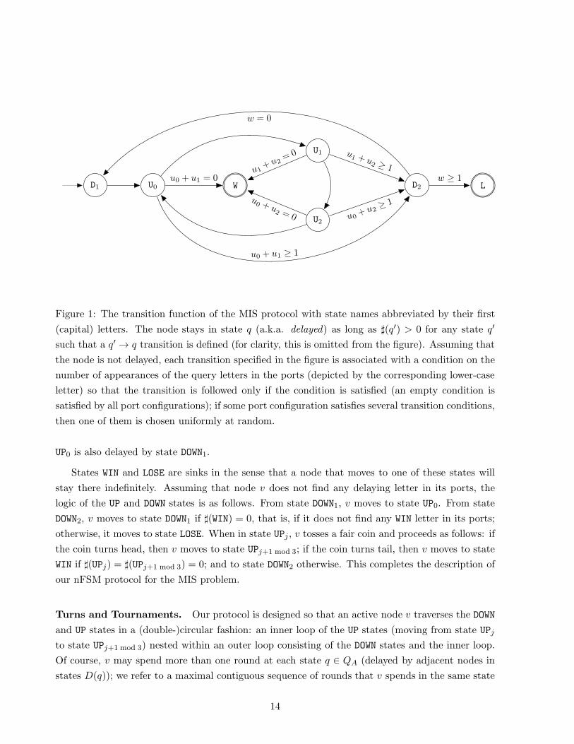
Figure 1: The transition function of the MIS protocol with state names abbreviated by their first

(capital) letters. The node stays in state q (a.k.a. delayed) as long as ♯(q′) > 0 for any state q′

such that a q′ → q transition is defined (for clarity, this is omitted from the figure). Assuming that

the node is not delayed, each transition specified in the figure is associated with a condition on the

number of appearances of the query letters in the ports (depicted by the corresponding lower-case

letter) so that the transition is followed only if the condition is satisfied (an empty condition is

satisfied by all port configurations); if some port configuration satisfies several transition conditions,

then one of them is chosen uniformly at random.

UP0 is also delayed by state DOWN1.

States WIN and LOSE are sinks in the sense that a node that moves to one of these states will

stay there indefinitely. Assuming that node v does not find any delaying letter in its ports, the

logic of the UP and DOWN states is as follows. From state DOWN1, v moves to state UP0. From state

DOWN2, v moves to state DOWN1 if ♯(WIN) = 0, that is, if it does not find any WIN letter in its ports;

otherwise, it moves to state LOSE. When in state UPj , v tosses a fair coin and proceeds as follows: if

the coin turns head, then v moves to state UPj+1 mod 3; if the coin turns tail, then v moves to state

WIN if ♯(UPj) = ♯(UPj+1 mod 3) = 0; and to state DOWN2 otherwise. This completes the description of

our nFSM protocol for the MIS problem.

Turns and Tournaments. Our protocol is designed so that an active node v traverses the DOWN

and UP states in a (double-)circular fashion: an inner loop of the UP states (moving from state UPj

to state UPj+1 mod 3) nested within an outer loop consisting of the DOWN states and the inner loop.

Of course, v may spend more than one round at each state q ∈ QA (delayed by adjacent nodes in

states D(q)); we refer to a maximal contiguous sequence of rounds that v spends in the same state

14

q ∈ QA as a q-turn, or simply as a turn if the actual state q is irrelevant. A maximal contiguous

sequence of turns that starts at a DOWN1-turn and does not include any other DOWN1-turn (i.e., a

single iteration of the outer loop) is referred to as a tournament. We index the tournaments and

the turns within a tournament by the positive integers. Note that by definition, every tournament

i of v starts with a DOWN1-turn, followed by a non-empty sequence of UP-turns. If tournament i+ 1

of v exists, then tournament i ends with a DOWN2-turn; otherwise, it ends with an UP-turn. The

following observation is established by induction on the rounds.

Observation 4.1. Consider some node v ∈ V in turn j ∈ Z>0 of tournament i ∈ Z>0 and some

active node u ∈ N (v).

• If this is a DOWN1-turn of v (j = 1), then u is in either (A) the last (DOWN2-)turn of tournament

i− 1; (B) turn 1 of tournament i; or (C) turn 2 of tournament i.

• If this is an UP-turn of v (j ≥ 2), then u is in either (A) turn j−1 of tournament i; (B) turn

j of tournament i; (C) turn j +1 of tournament i; or (D) the last (DOWN2-)turn j′ ≤ j +1 of

tournament i.

• If this is a DOWN2-turn of v (the last turn of this tournament), then u is in either (A) an

UP-turn j′ ≥ j − 1 of tournament i; (B) the last (DOWN2-)turn of tournament i; or (C) turn 1

of tournament i+ 1.

Given some U ⊆ V and i, j ∈ Z>0, let TU (i, j) denote the first time at which every node v ∈ Usatisfies either

(1) v is inactive;

(2) v is in tournament i′ > i;

(3) v is in the last (DOWN2-)turn of tournament i; or

(4) v is in turn j′ ≥ j of tournament i.

Employing Observation 4.1, the delaying states feature guarantees that

Tv(i, j + 1) ≤ TN (v)∪v(i, j) + 1 (1)

for every v ∈ V and i, j ∈ Z>0. Since TU (i, j) ≤ TV (i, j) for every U ⊆ V , we can apply inequal-

ity (1) to each node v ∈ V , concluding that

TV (i, j + 1) ≤ TV (i, j) + 1 ,

which immediately implies that

TV (i, k + 1) ≤ TV (i, 1) + k . (2)

Geometric Random Variables. Consider some v ∈ V and i ∈ Z>0. Assuming that tournament

i of v exists, let Xv(i) denote its length in terms of number of turns. For the sake of simplifying the

analysis, if tournament i is the last tournament of v, then we actually take Xv(i) to be its length plus

15

1 (this is done in order to compensate for the missing DOWN2-turn in the end of the tournament.) The

logic of the UP states implies that Xv(i) is a random variable that obeys distribution Geom(1/2)+2,

namely, a fixed term of 2 plus the geometric distribution with parameter 1/2, independently of

Xv′(i′) for any v′ 6= v and/or i′ 6= i. Since the maximum of n independent Geom(1/2)-random

variables is O(log n) with high probability, inequality 2 yields the following observation.

Observation 4.2. For every i ∈ Z>0, TV (i, 1) is finite with probability 1 and

TV (i+ 1, 1) ≤ TV (i, 1) +O(log n)

with high probability.

Our protocol is designed so that node v moves to an output state (WIN or LOSE) in the end

of each tournament with positive probability. Moreover, the logic of state DOWN2 guarantees that

if node v moves to state WIN in the end of tournament i, then all its active neighbors move to

state LOSE in the end of their respective tournaments i. By Observation 4.2, we conclude that our

protocol reaches an output configuration with probability 1 and that every output configuration

reflects an MIS. It remains to bound the run-time of our protocol.

The Virtual Graph Gi. Let V i be the set of nodes for which tournament i exists and let

Gi = (V i, Ei) be the subgraph induced on G by V i, where Ei = E ∩ (V i × V i).10 Given some

node v ∈ V i, let N i(v) = u ∈ V i | (u, v) ∈ E be the neighborhood of node v in Gi and let

di(v) = |N i(v)| be its degree. Note that the graph Gi is virtual and defined solely for the sake

of the analysis; in particular, we do not assume that there exists some time at which the graph

induced by any meaningful subset of the nodes (say, the nodes in tournament i) agrees with Gi.

The key observation in this context is that conditioned on Gi, the random variables Xv(i), v ∈ V i,

are (still) independent and obey distribution Geom(1/2) + 2. Moreover, the graph Gi+1 is fully

determined by the random variables Xv(i), v ∈ V i. Our analysis relies on the following lemma.

Lemma 4.3. There exist two constants 0 < p, c < 1 such that |Ei+1| ≤ c|Ei| with probability at

least p.

We will soon turn to proving Lemma 4.3, but first, let us explain why it suffices for the comple-

tion of our analysis. Define the random variable Y = mini ∈ Z>0 : |Ei| = 0. Lemma 4.3 implies

that Y is stochastically dominated by a random variable that obeys distribution NB(O(log n), 1−p)+O(log n), namely, a fixed term of O(log n) plus the negative binomial distribution with param-

eters O(log n) and 1 − p, hence Y = O(log n) in expectation and with high probability. Since the

nodes in V − V i are all in an output state (and will remain in that state), and since the logic of

the UP states implies that a degree-0 node in Gi will move to state WIN in the end of tournament

i (with probability 1) and thus, will not be included in V i+1, we can employ Observation 4.2 to

conclude that the run-time of our protocol is O(log2 n).

10 The notation Gi used in this section should not be confused with the ith power of G.

16

The remainder of this section is dedicated to establishing Lemma 4.3. The proof technique we

use for that purpose resembles (a hybrid of) the techniques used in [3] and [29] for the analysis of

their MIS algorithms. We say that node v ∈ V i is good in Gi if

|u ∈ N i(v) | di(u) ≤ di(v)| ≥ di(v)/3 ,

i.e., if at least third of v’s neighbors in Gi have degrees smaller or equal to that of v. The following

lemma is established in [3].

Lemma 4.4 ([3]). More than half of the edges in Ei are incident on good nodes in Gi.

Disjoint Winning Events. Consider some good node v in Gi with d = di(v) > 0 and let N i(v) =

u ∈ N i(v) | di(u) ≤ d. Recall that the definition of a good node implies that |N i(v)| ≥ d/3. We

say that node u ∈ N i(v) wins v in tournament i if

Xu(i) > maxXw(i) | w ∈ N i(u) ∪ N i(v)− u

and denote this event by Ai(u, v). The main observation now is that if u wins v in tournament i,

then in the end of their respective tournaments i, u moves to state WIN and v moves to state LOSE.

Moreover, the events Ai(u, v) and Ai(w, v) are disjoint for every u,w ∈ N i(v), u 6= w.

Let u1, . . . , uk be the nodes in N i(u) ∪ N i(v), where 0 < k ≤ 2 d by the definition of a good

node. Let Bi(u, v) denote the event that the maximum of Xuℓ(i) | 1 ≤ ℓ ≤ k is attained at a

single 1 ≤ ℓ ≤ k. Since Xu1(i), . . . ,Xuk

(i) are independent random variables that obey distribution

Geom(1/2) + 2, it follows that P(Bi(u, v)) ≥ 2/3. Therefore,

P(Ai(u, v)

)= P

(Ai(u, v) | Bi(u, v)

)· P

(Bi(u, v)

)≥ 1

k· 23,

which implies that

P(v /∈ V i+1 | v is good in Gi

)≥ P

∨

u∈N i(v)

Ai(u, v)

=∑

u∈N i(v)

P(Ai(u, v)

)≥ d

3· 1

2 d· 23

=1

9.

Combined with Lemma 4.4, we conclude that E[|Ei+1|] < 3536 |Ei|. Lemma 4.3 follows by Markov’s

bound.

Theorem 4.5. There exists an nFSM protocol that computes an MIS in any n-node graph with

run-time O(log2 n).

5 Coloring a Tree with 3 Colors

Given a graph G = (V,E), the coloring problem asks for an assignment of colors to the nodes such

that no two neighboring nodes have the same color. A coloring using at most k colors is called a

17

k-coloring. The smallest number of colors needed to color graph G is called its chromatic number,

denoted by χ(G). In general, χ(G) is difficult to compute even in a centralized model [10]. As such,

the distributed computing community is generally satisfied already with a (∆+1)-, O(∆)-, or even

∆O(1)-coloring, where ∆ = ∆(G) is the largest degree in the graph G, with possibly ∆(G)≫ χ(G)

[15, 32, 19, 26, 37, 7, 22, 9, 8, 35]. However, even for relatively simple graph classes, ∆ may grow

with n. As the output of each node under the nFSM model is taken from a constant size set, we

must and will tackle a graph class that features a small chromatic number: trees.

Any tree T has a chromatic number χ(T ) = 2. Unfortunately, it is easy to show that in general,

the task of 2-coloring trees requires run-time proportional to the diameter of the tree even under the

message passing model, and hence cannot be achieved by an efficient distributed algorithm. The

situation improves dramatically once 3 colors are allowed; indeed, Cole and Vishkin [15] presented

a distributed algorithm that 3-colors directed paths, and in fact, any directed tree (directed in the

sense that each node knows the port leading to its unique parent), in time O(log∗ n). Linial [26]

showed that this is asymptotically optimal.

Since it is not clear how to represent directed trees in the nFSM model, we focus on undirected

trees, designing an nFSM protocol that 3-colors any n-node (undirected) tree in run-time O(log n).

A lower bound result of Kothapalli et al. [21] shows that this cannot be improved (asymptotically)

even by a message passing algorithm as long as the size of each message is O(1).

Employing Theorems 3.1 and 3.4, we assume a locally synchronous environment and use

multiple-letter queries. The description of the protocol will not dwell into the level of defining

the states and transition function (as we did in Section 4 for the MIS protocol), but the reader will

be easily convinced that this protocol can indeed be implemented under the nFSM model.

The Modes. At all times, each node v ∈ V is in one of the following three modes.

(1) Mode COLORED: the color of v is determined (v is in an output state) and it no longer takes an

active part in the protocol.

(2) Mode ACTIVE: the color of v has not been determined yet and v takes an active part in the

protocol.

(3) Mode WAITING: the color of v has not been determined yet and v is waiting for one of its

neighbors to be colored before it resumes taking an active part in the protocol (going back to mode

ACTIVE).

Initially, all nodes are in mode ACTIVE. When an ACTIVE node moves to mode COLORED, as-

signed with color c ∈ 1, 2, 3, it transmits a ‘my color is c’ message and it does not transmit any

more messages; when an ACTIVE node moves to mode WAITING, it transmits an ‘I am WAITING’

message and it does not transmit any more messages until it returns to mode ACTIVE, in which

case it transmits an ‘I am ACTIVE’ message. Therefore, the message stored in the port of node v

18

corresponding to neighbor u of v always indicates (perhaps among other things) the current mode

of u.

The Phases. The execution of the protocol is divided into phases indexed by the positive integers,

where each phase consists of 4 rounds. Consider some phase i ∈ Z>0. Let Vi be the set of ACTIVE

nodes at the beginning of phase i and let F i be the forest induced on T by V i (F i may contain one

or more trees), referred to as the ACTIVE forest. Given some node v ∈ V i, let N i(v) = u ∈ V i |(u, v) ∈ E be the neighborhood of v in F i and let di(v) = |N i(v)| be its degree.

The structure of the phases is as follows. Consider some node v ∈ V i. In round 1 of the

phase, v transmits an ‘I am ACTIVE’ message. Setting the bounding parameter of the protocol to

b = 3, we conclude that in round 2, v can distinguish between the cases di(v) = 0, di(v) = 1,

di(v) = 2, and di(v) ≥ 3 simply by querying its ports for ‘I am ACTIVE’ messages; in other words,

v “knows” f3(di(v)), i.e., its degree calculated with respect to the one-two-many principle with

bounding parameter b = 3. Employing this “knowledge”, v transmits f3(di(v)) in round 2 of phase

i, so in round 3, the port of v corresponding to u stores a message indicating f3(di(u)) for every

node u ∈ N i(v).

Rounds 3 and 4 of phase i are dedicated to Procedure RandColor that we will describe soon.

Whether or not v runs Procedure RandColor depends on the degree of v and on the degrees of its

ACTIVE neighbors. Specifically, v runs Procedure RandColor if: (1) di(v) = 0; (2) di(v) = 1 with

N i(v) = u and di(u) = 1; or (3) di(v) = 2 with N i(v) = u1, u2 and di(u1), di(u2) ≤ 2. In

contrast, if di(v) = 1 with N i(v) = u and di(u) ≥ 2, then v moves to mode WAITING without

running Procedure RandColor, in which case we say (just for the sake of the analysis) that v waits

on u. Otherwise (di(v) ≥ 3 or di(v) = 2 with some neighbor u ∈ N i(v) such that di(u) ≥ 3), v

remains in mode ACTIVE without running Procedure RandColor.

As stated beforehand, the COLORED nodes do not take an active part in the protocol. A WAITING

node v moves to mode ACTIVE in the end of phase i if some neighbor u of v, u ∈ V i, moves to mode

COLORED during phase i (v spots this event by querying on ‘my color is c’ messages).

Procedure RandColor. Responsible for the actual color assignments, Procedure RandColor takes

2 rounds (rounds 3 and 4 of some phase). Only an ACTIVE node may run the procedure, and when

the procedure is over, the node either stays in mode ACTIVE or moves to mode COLORED. Consider

some node v running the procedure and let C(v) ⊆ 1, 2, 3 be the subset of colors which are not

yet assigned to the neighbors of v in T . (Our analysis shows that if v is ACTIVE, then C(v) 6= ∅.)As every COLORED node transmits a message indicating its color, v can determine C(v) by querying

its ports.

In the first round of Procedure RandColor, v picks some color c ∈ C(v) uniformly at random

and transmits a ‘proposing color c’ message. In the second round of the procedure, if v finds a

19

‘proposing color c’ (with the same c) in its ports, then it remains in mode ACTIVE. Otherwise (no

neighbor of v competes with v over color c), it moves to mode COLORED and transmits a ‘my color

is c’ message. This completes the description of our protocol.

The Waiting Hierarchy. The ‘waits on’ relation induces a hierarchy referred to as the waiting

hierarchy which is represented by a (collection of) directed tree(s) defined over a subset of the edges

of the tree T . Our protocol is designed so that if v waits on u, moving to mode WAITING in phase i,

then in phases 1, . . . , i, u was ACTIVE, and in phase i+1, u is either ACTIVE or COLORED. Moreover,

if u is ACTIVE and v ∈ N (u) is WAITING, then v must be waiting on u. Note also that if v waits on

u and u moves to mode COLORED in phase j, then v moves back to mode ACTIVE in (the beginning

of) phase j + 1 and dj+1(v) = 0.

Observation. In the beginning of phase i, |C(v)| ≥ mindi(v) + 1, 3 for every i ∈ Z>0 and node

v ∈ V i.

Proof. As long as di(v) ≥ 3, no neighbor of v can run Procedure RandColor, and hence no neighbor

of v can move to mode COLORED. Therefore, C(v) = 1, 2, 3 in the beginning of the first phase

i ∈ Z>0 such that di(v) ≤ 2. From that moment on, every ACTIVE neighbor of v that moves to

mode COLORED decreases both |C(v)| and di(v) by 1. The assertion is completed by recalling that

non-ACTIVE neighbors of v must be waiting on v and hence, cannot move to mode COLORED before

v does.

Corollary 5.1. Consider some node v ∈ V i that runs Procedure RandColor. If di(v) = 0, then

v moves to mode COLORED with probability 1. Otherwise (di(v) is either 1 or 2), v moves to mode

COLORED with a positive constant probability.

Let V i be the restriction of V i to nodes v that were ACTIVE in all phases 1, . . . , i; this is, V i does

not include WAITING nodes that became ACTIVE again (recall that these will move to mode COLORED

in the next phase with probability 1). Let F i be the forest induced on T by V i. Given some node

v ∈ V i, let N i(v) = u ∈ V i | (u, v) ∈ E be the neighborhood of v in F i and let di(v) = |N i(v)|be its degree. Observe that if v ∈ V i, then v ∈ V i and di(v) = di(v). Therefore, if v ∈ V i − V i,

then di(v) = 0, in which case v runs Procedure RandColor in phase i and Corollary 5.1 guarantees

that v /∈ V i+1.

The correctness of the protocol can now be established: The logic of Procedure RandColor

implies that every output configuration is a legal coloring. Since ACTIVE leaves are removed from

F i with probability 1 and since every tree has at least two leaves, it follows that V 1+k = ∅ for

k = ⌈n/2⌉. Combining the properties of the waiting hierarchy with Corollary 5.1, we conclude that

the execution reaches an output configuration within at most k additional phases. It remains to

analyze the run-time of our protocol.

20

Good nodes. Consider some tree T ′. We say that node v of T ′ is good if v is a leaf or if the

degree of v is 2 and both neighbors of v are of degree at most 2.

Observation 5.2. In every tree, at least a (1/5)-fraction of the nodes are good.

Consider some i ∈ Z>0 and some node v ∈ V i. Let T ′ be the tree to which v belongs in F i.

We argue that if v is good in T ′, then v /∈ V i with a positive constant probability. Indeed, if v

is a leaf in T ′, which means that di(v) = di(v) = 1, then it either moves to mode WAITING with

probability 1 (if the neighbor of v has a higher degree) or it runs Procedure RandColor, in which

case Corollary 5.1 guarantees that v moves to mode COLORED with a positive constant probability;

if di(v) = di(v) = 2 and both neighbors of v in F i (and in T ′) are of degree at most 2, then v runs

Procedure RandColor, in which case Corollary 5.1 again guarantees that v moves to mode COLORED

with a positive constant probability. Since Corollary 5.1 also guarantees that nodes of degree 0 in

F i move to mode COLORED with probability 1, we can employ Observation 5.2 and Markov’s bound

to establish the following observation.

Observation 5.3. There exists two constants 0 < p, c < 1 such that |V i+1| ≤ c|V i| with probability

at least p.

Similarly to the analysis in Section 4, define the random variable Y = mini ∈ Z>0 : |V i| =0. Observation 5.3 implies that Y is stochastically dominated by a random variable that obeys

distribution NB(O(log n), 1 − p) + O(log n), namely, a fixed term of O(log n) plus the negative

binomial distribution with parameters O(log n) and 1− p, hence Y = O(log n) in expectation and

with high probability. Since Y bounds from above the depth of the waiting hierarchy, it follows

that the execution reaches an output configuration within 2Y phases, which completes the analysis.

Theorem 5.4. There exists an nFSM protocol that 3-colors any n-node (undirected) tree with

run-time O(log n).

6 Computational Power

A deterministic linear bounded automaton (dLBA) is a (deterministic) Turing machine whose work-

ing tape is restricted to the cells specifying the input (this is equivalent to a DSPACE(O(n)) Turing

machine). A non-deterministic linear bounded automaton, a.k.a., linear bounded automaton (LBA),

is the non-deterministic version of a dLBA, and a randomized linear bounded automaton (rLBA)

is the randomized version. Kuroda [24] proved that the class of languages that can be decided

by an LBA is exactly the context-sensitive languages, corresponding to the Type-1 grammars in

Chomsky’s hierarchy of formal languages [14]. Whether LBAs are equivalent to dLBAs and where

exactly do rLBAs lie between the two are major open questions in computational complexity (cf.

the first LBA problem). The following two lemmas show that in terms of its computational power

(regardless of run-time considerations), an nFSM protocol is essentially equivalent to an rLBA.

Lemma 6.1. An nFSM protocol on a graph G of arbitrary topology can be simulated by an rLBA.

21

Proof. The input for the Turing machine is the graph G, given as an adjacency list. In order to

simulate the execution of the nFSM protocol, we store some additional information in the entries

of the adjacency list as follows: For each node v, we store its current state and the next letter

it transmits. For every node u in the list of neighbors N(v) attached to v, we store the entry

of u’s port that corresponds to v. In each round of the nFSM protocol, the rLBA performs two

sweeps of the list of nodes: The first sweep serves to calculate v’s next state q and transmitted

letter σ for all nodes v, based on v’s current state and the messages in its ports, according to the

nFSM state machine, which is hard-wired in the rLBA. However, the calculated letter σ is not

being “transmitted” yet, so the calculations for subsequent nodes in the list are not messed up,

but rather stored in the corresponding place next to v. In the second sweep, for every node v, the

letter σ is being “transmitted”, that is, the lists of neighbors are traversed, and at each occurrence

of v, the current letter is replaced by σ. This way, we simulate every round of the nFSM protocol.

In total, our simulation requires additional O(1) space per node and O(1) space per edge, hence it

can be implemented with an rLBA. The assertion follows.

Lemma 6.2. An rLBA can be simulated by an nFSM protocol on a path.

Proof. Let n be the number of cells in the tape of the rLBA. Then, the path network has n nodes,

each corresponding to one cell of the tape, i.e., we identify a node v of the path nFSM with a

certain cell on the tape. Let Γ be the working alphabet and P be the state space of the rLBA. The

nFSM protocol is designed so that the state of node v indicates: (1) which letter from Γ is written

in v; (2) if the head of the rLBA currently points to v; (3) the current state of the rLBA, which is

allowed to be incorrect if (2) is false; and (4) if the head is currently located to the left or to the

right of v. Hence, we fix Q = Γ×0, 1×P ×L,R. The alphabet of the nFSM is Σ = L,R×P .

Suppose that the input to the rLBA is γ1 . . . γn ∈ Γn. Then, we assume that the initial state of

the ith node in the path is (γi, h, p0, L), where p0 is the initial state of the Turing machine and

h =

1 if i = 1

0 if i > 1 .

Note that the distinction between the initial state of the first node in the path and the initial states

of all other nodes is without loss of generality. Indeed, as the first and last nodes have degree 1

and all interior nodes have degree 2, it is easy for a node to “decide” (under the nFSM model) if

it is an interior node. Distinguishing between the first and last nodes is unavoidable if one wants

to distinguish between the inputs γ1 . . . γn and γn . . . γ1.

At all times, we maintain the invariant that exactly one node is in a state in Γ×1×P ×L,R— denote this node as active — whereas all other nodes are in a state in Γ×0×P ×L,R. Only

the active node can transmits messages; all other nodes remain silent and listen. If an non-active

node v receives a message indicating that the head should move to the left (respectively, right),

and v’s state indicates that the head is currently to its right (resp., left), then v becomes the active

22

node; otherwise, v does not react to this message. Now, the nodes simulate the behavior of the

rLBA by calculating the next state of the rLBA based on the rLBA’s transition function (which is

hard-wired in the FSM) and updating their own states accordingly. The assertion follows.

23

References

[1] Y. Afek, N. Alon, Z. Bar-Joseph, A. Cornejo, B. Haeupler, and F. Kuhn. Beeping a maximal

independent set. In Proceedings of the 25th international conference on Distributed computing

(DISC), pages 32–50, 2011.

[2] Y. Afek, N. Alon, O. Barad, E. Hornstein, N. Barkai, and Z. Bar-Joseph. A Biological Solution

to a Fundamental Distributed Computing Problem. Science, 331(6014):183–185, Jan. 2011.

[3] N. Alon, L. Babai, and A. Itai. A fast and simple randomized parallel algorithm for the

maximal independent set problem. J. Algorithms, 7:567–583, December 1986.

[4] B. Awerbuch. Complexity of network synchronization. J. ACM, 32(4):804–823, 1985.

[5] B. Awerbuch, B. Patt-Shamir, D. Peleg, and M. E. Saks. Adapting to asynchronous dynamic

networks (extended abstract). In STOC, pages 557–570, 1992.

[6] B. Awerbuch and D. Peleg. Network synchronization with polylogarithmic overhead. In FOCS,

pages 514–522, 1990.

[7] L. Barenboim and M. Elkin. Distributed (delta+1)-coloring in linear (in delta) time. In STOC,

pages 111–120, 2009.

[8] L. Barenboim and M. Elkin. Combinatorial algorithms for distributed graph coloring. In

DISC, pages 66–81, 2011.

[9] L. Barenboim and M. Elkin. Deterministic distributed vertex coloring in polylogarithmic time.

J. ACM, 58(5):23, 2011.

[10] M. Bellare, O. Goldreich, and M. Sudan. Free bits, pcps, and nonapproximability-towards

tight results. SIAM J. Comput., 27(3):804–915, 1998.

[11] Y. Benenson, T. Paz-Elizur, R. Adar, E. Keinan, Z. Livneh, and E. Shapiro. Programmable

and autonomous computing machine made of biomolecules. Nature, 414(6862):430–434, Nov.

2001.

[12] D. Brand and P. Zafiropulo. On communicating finite-state machines. J. ACM, 30:323–342,

April 1983.

[13] I. Chlamtac and S. Kutten. On Broadcasting in Radio Networks–Problem Analysis and Pro-

tocol Design. Communications, IEEE Transactions on [legacy, pre - 1988], 33(12):1240–1246,

1985.

[14] N. Chomsky. Three models for the description of language. IRE Transactions on Information

Theory, 2:113–124, 1956. http://www.chomsky.info/articles/195609--.pdf.

[15] R. Cole and U. Vishkin. Deterministic coin tossing with applications to optimal parallel list

ranking. Inf. Control, 70(1):32–53, July 1986.

[16] A. Cornejo and F. Kuhn. Deploying wireless networks with beeps. In Proceedings of the 24th

international conference on Distributed computing (DISC), pages 148–162, 2010.

[17] R. Flury and R. Wattenhofer. Slotted Programming for Sensor Networks. In International

Conference on Information Processing in Sensor Networks (IPSN), Stockholm, Sweden, April

2010.

[18] M. Gardner. The fantastic combinations of John Conway’s new solitaire game ‘life’. Scientific

American, 223(4):120–123, 1970.

[19] A. V. Goldberg, S. A. Plotkin, and G. E. Shannon. Parallel symmetry-breaking in sparse

graphs. SIAM J. Discrete Math., 1(4):434–446, 1988.

[20] P. Gordon. Numerical Cognition Without Words: Evidence from Amazonia. Science,

306(5695):496–499, Oct. 2004.

[21] K. Kothapalli, C. Scheideler, M. Onus, and C. Schindelhauer. Distributed Coloring in

O(√log n) Bit Rounds. In 20th International Parallel and Distributed Processing Symposium

(IPDPS), 2006.

[22] F. Kuhn. Weak graph colorings: distributed algorithms and applications. In Proceedings of

the twenty-first annual symposium on Parallelism in algorithms and architectures, SPAA ’09,

pages 138–144, New York, NY, USA, 2009. ACM.

[23] F. Kuhn, T. Moscibroda, and R. Wattenhofer. What cannot be computed locally! In Pro-

ceedings of the twenty-third annual ACM symposium on Principles of distributed computing

(PODC), pages 300–309, 2004.

[24] S.-Y. Kuroda. Classes of languages and linear-bounded automata. Information and Control,

7(2):207–223, 1964.

[25] C. Lenzen and R. Wattenhofer. MIS on trees. In Proceedings of the 30th annual ACM SIGACT-

SIGOPS symposium on Principles of distributed computing (PODC), pages 41–48, New York,

NY, USA, 2011.

[26] N. Linial. Locality in distributed graph algorithms. SIAM J. Comput., 21:193–201, Feb. 1992.

[27] M. Luby. A simple parallel algorithm for the maximal independent set problem. SIAM J.

Comput., 15:1036–1055, November 1986.

[28] N. A. Lynch. Distributed Algorithms. Morgan Kaufmann, 1st edition, 1996.

[29] Y. Metivier, J. M. Robson, N. Saheb-Djahromi, and A. Zemmari. An optimal bit complexity

randomised distributed MIS algorithm. Distributed Computing, 23(5-6):331–340, Jan. 2011.

[30] J. V. Neumann. Theory of Self-Reproducing Automata. University of Illinois Press, Champaign,

IL, USA, 1966.

[31] D. Peleg. Distributed computing: a locality-sensitive approach. Society for Industrial and

Applied Mathematics, Philadelphia, PA, USA, 2000.

[32] S. Plotkin. Graph-theoretic techniques for parallel, distributed, and sequential computation.

MIT/LCS/TR. Laboratory for Computer Science, Massachusetts Institute of Technology, 1988.

[33] D. Sadava. Life: The Science of Biology. Sinauer Associates, 2011.

[34] J. Schneider and R. Wattenhofer. An Optimal Maximal Independent Set Algorithm for

Bounded-Independence Graphs. In Journal of Distributed Computing, March 2010.

[35] J. Schneider and R. Wattenhofer. Distributed Coloring Depending on the Chromatic Number

or the Neighborhood Growth. In 18th International Colloquium on Structural Information and

Communication Complexity (SIROCCO), Poland, June 2011.

[36] J. Suomela. Survey of local algorithms. To appear in: ACM Computing Surveys, 2012.

http://www.cs.helsinki.fi/u/josuomel/doc/local-survey.pdf.

[37] M. Szegedy and S. Vishwanathan. Locality based graph coloring. In STOC, pages 201–207,

1993.

[38] S. Wolfram. A new kind of science. Wolfram Media, Champaign, Illinois, 2002.