CLIMATE RESEARCHClim Res

Vol. 47: 187–199, 2011doi: 10.3354/cr01003

Published online June 30

1. INTRODUCTION

Extreme hot weather and climate phenomena areareas of great research interest, since increases intheir frequency and severity can cause considerabledamage to ecosystems and human society. The focusof the present study is on stochastic characterizationof hot weather spells in southern Quebec, where mostof the population of the province is concentrated andwhere high daily maximum temperatures, reaching>30°C over various durations, during the summerseason have occasionally been experienced (Khaliq et

al. 2005). Extended episodes of such high tempera-tures and increases in their rate of occurrence underthe anticipated climate change scenarios could con-siderably impact public health and socio-economicsectors.

Episodes of hot weather persisting over a certainnumber of days are termed hot weather events(HWEs) in the present study. Thus, in general, anHWE in volves the occurrence of consecutive days ofhigh temperatures, along with high levels of relativehumidity. The high temperatures could be in the formof either daily maximum temperature (henceforth,

© Inter-Research 2011 · www.int-res.com*Email: naveed.khaliq@ec.gc.ca

Stochastic modeling of hot weather spells and theircharacteristics

M. N. Khaliq1,*, T. B. M. J. Ouarda2, P. Gachon1, L. Sushama3

1Adaptation and Impacts Research Section, Atmospheric Science and Technology Directorate, Environment Canada, Place Bonaventure, Northeast Tower, 800 Gauchetiere Street West, Office 7810, Montreal, Quebec H5A 1L9, Canada

2INRS-ETE, University of Quebec, 490 de la Couronne, Quebec City, Quebec G1K 9A9, Canada3Centre ESCER, University of Quebec at Montreal, Quebec H3C 3P8, Canada

ABSTRACT: Stochastic characterization of hot weather events (HWEs) is useful for developing prob-abilistic climate change information. We assumed that simultaneous exceedances of daily minimumand maximum temperatures (i.e. Tmin and Tmax, respectively), above the selected thresholds for thesetemperatures, form alternating sequences of ‘hot weather’ and ‘non-hot weather’ spells. This behav-ior is stochastically characterized by a generalization of the compound Poisson process. The general-ization is achieved by randomizing the mean rate of occurrence of the original Poisson process withthe gamma distribution. The resulting compound Poisson process gamma (CPPG) model consists of 2basic components: one relates to the occurrence of HWEs and the other to their durations. Detailedvalidation of the CPPG model is presented for HWEs derived from homogenized Tmin and Tmax obser-vations from McTavish station (located in the centre of Montreal, southern Quebec, Canada) for theJune–August hot summer season over the period 1941–2000. Results of the study suggest that theCPPG model can adequately describe occurrences of HWEs and the distributions of their durations(including distributions of extreme durations), as well as the distributions of the number of hot days,when assessed on the basis of the Kolmogorov-Smirnov and chi-squared goodness-of-fit tests. A non-stationary framework is introduced and applied to 2 contrasting sets of non-stationary observations ofHWEs from Les Cedres and La Tuque (southern Quebec) for the 1941–2000 period. The results of thenon-stationary modeling approach demonstrate that the developed methodology is generally applic-able and could be useful in developing probabilistic information about various characteristics of hotweather climate for a particular location or a larger spatial domain.

KEY WORDS: Climate change · Compound Poisson process · Hot weather spells · Logarithmic distribution · Negative binomial distribution · Poisson-gamma model

Resale or republication not permitted without written consent of the publisher

Clim Res 47: 187–199, 2011188

denoted Tmax) or daily minimum temperature (hence-forth, denoted Tmin) or the 2 together. There is no uni-fied definition of an HWE, and its choice dependsupon a number of factors, e.g. the type and length ofthe available data, the chosen sector impacted byHWEs (i.e. public health, agriculture, wildlife, socio-economics, etc.), the time of year, local exacerbatingforcing factors, etc. We define an HWE as an extremeclimate event when—over a specific period—bothTmin and Tmax values are above relatively high chosenthresholds (see Section 3). These types of hot weatherspells are supposedly more severe, in relation to theirimpact on public health and socio-economic sectors,than spells defined on the basis of Tmin or Tmax alone,such as in Katsoulis & Hatzianastassiou (2005), Khaliqet al. (2005) and Furrer et al. (2010). As in Khaliq et al.(2006a, 2007), homogenized Tmin and Tmax observa-tions for the June–August hot summer season areemployed to derive HWEs. The effect of relativehumidity, for which homogenized observations arenot yet available, is not taken into account. However,inclusion of a relative humidity factor in the definitionof an HWE would certainly be useful, since HWEs arelikely more detrimental to humans under conditions ofincreased atmospheric moisture.

Following the above definition of an HWE, simulta-neous observations of Tmin and Tmax would result inalternate sequences of ‘hot weather’ and ‘non-hotweather’ spells. In a very general manner, thesesequences can be stochastically modeled using pointprocess approaches (Cox & Isham 1980, Guttorp1995). In these approaches, the primary mechanism ofevent occurrences is usually assumed to follow a Pois-son process, which is compounded with other sec-ondary processes to formulate compound Poisson pro-cesses. Various forms of the compound Poissonprocess have been successfully used for modelinghydro-climatological data (e.g. rainfall, Rodriguez-Iturbe et al. 1987; drought, Zelenhasic & Salvai 1987,Abaurrea & Cebrián 2002; wind storms, Rootzén &Tajvidi 1997; hurricanes, Elsner & Bossak 2001, Katz2002; very cold days, Prieto et al. 2004; hot spells, Fur-rer et al. 2010). However, in practice, one couldencounter situations where the assumptions of thePoisson process (e.g. equality of mean and varianceproperty) may not be satisfied or they may holdmerely in a weak manner. In such situations, the orig-inal Poisson process needs to be modified, particularlyto account for over-dispersion in the event occurrenceprocess; this is also the case in the present study. Thepresent study has 2 main objectives. (1) To de velop astochastic characterization of hot weather climateusing the compound Poisson process gamma (CPPG)model — a generalization of the Poisson process thatreduces to the original form as a limiting case; gamma

is the distribution of the rate parameter of the Poissonprocess. (2) To develop a plausible non-stationaryprobabilistic framework for hot weather activity insouthern Quebec using data from 3 selected locations(Montreal, Les Cedres and La Tuque) with quite con-trasting features of HWE occurrences and their char-acteristics.

2. MODEL COMPONENTS

In the present study, hot weather spells are charac-terized in terms of 4 components: (1) HWE occur-rences, (2) HWE durations, (3) the number of hot daysand (4) the longest duration of HWEs. The first 2 com-ponents (termed basic components) are explicitly mod-eled, while the distributions of the latter 2 are derivedfrom those of the first 2. Other characteristics, like theintensity of HWEs (for example, represented in termsof the maximum temperature associated with a HWE)is not addressed explicitly in this study, but could beattempted in the future following the approachesdescribed in Katsoulis & Hatzianastassiou (2005) andFurrer et al. (2010) or their suitable variants in a multi-variate framework. The 4 components, described be -low one at a time, correspond to the characteristics ofHWEs for the June–August summer season.

2.1. HWE occurrences

It is assumed that the occurrence of HWEs follows aPoisson process {N }, denoting the number of eventsoccurring within the time interval (0, t), i.e. within theJune–August (JJA) summer season of each year. Thenumber of events in any interval of time is indepen-dent of the number of events in any other non- overlapping interval of time. The random variable Nhas a Poisson distribution with a mean rate λ. That is,the probability P of n events occurring within the inter-val (0, t) can be expressed as:

(1)

The mean μN and variance σ2N of N are equal and are

given by μN = σ2N = λ. In particular, for the case of rare

events (i.e. the HWEs corresponding to relatively highvalues of Tmin and Tmax thresholds; see Section 3.2), therequirement of the equality of the mean and varianceproperty of the Poisson distribution is not satisfied andthe event occurrence process results in over-disper-sion, i.e. σ2

N is significantly greater than μN. To accountfor over-dispersion, generally the para meter of thePoisson distribution is assumed to follow a gamma dis-tribution (Cameron & Trivedi 1998, Medhi 2002), withthe density function given by:

P N n n nn( ) e 0,1, 2, ...= = =−λ λ( ) / !,

Khaliq et al.: Stochastic modeling of hot weather spells

(2)

where α > 0 and 1/β > 0 are, respectively, the shapeand scale parameters and Γ(.) is the gamma function.With this assumption, the distribution of N becomes:

(3)

which is an extended negative binomial distributionwith parameter p = β/(1 + β) and r = α in the form ofcommonly used notation. This formulation is knownas a Poisson-gamma or Poisson mixture model in thestatistical literature (e.g. Skinner 1992, Cameron &Tri vedi 1998). For the Poisson-gamma model, μN =r (1 – p)/ p and σ2

N = r (1 – p)/ p2. Thus, over-dispersedcases can be easily modeled by estimating the para-meters p and r using either the method of maximumlikelihood or the method of moments for which therelationships for both the mean and variance need tobe employed. An intuitively appealing explanationfor the use of the Poisson-gamma model for HWEoccurrences could be that: (1) it accommodates anyrandom effect or heterogeneity (e.g. due to a season-ality effect on the rate of occurrence of HWEs), and(2) it reduces to the original Poisson process model asa limiting case, i.e. when the parameter p approachesunity.

2.2. Durations of HWEs

Let Xi > 0 denote the duration of HWE associatedwith the i th occurrence, i = 1, 2, 3, …, within the JJAsummer season of each year and assume that the Xisare independent and identically distributed. Let thecommon cumulative distribution function be denotedby Fx(x) = P(X ≤ x), with mean μX and variance σ2

N,and further, assume that the duration process {X } isstatistically independent of the occurrence process{N }. The joint process, consisting of {X } in combina-tion with {N }, is referred to as the compound Poissonprocess or a ‘marked’ Poisson process, i.e. the dura-tion associated with an event occurrence is viewed asa mark; for additional explanations, see Cox & Isham(1980) and Guttorp (1995). The randomized com-pound Poisson process could be viewed as an exten-sion or a variant of the basic compound Poisson pro-cess. In practice FX(x) would be some positivelyskewed dis tribution function, such as the exponential,gamma, or lognormal from continuous distributionfamilies and the truncated geometric, negative bino-mial, or logarithmic from discrete distribution families.

During a preliminary analysis, 3 single-parameter dis-tributions (exponential, logarithmic and truncatedgeometric) were considered to identify strong candi-date distributions for modeling HWE durations. Theexponential is a continuous distribution, while theother 2 are discrete. The exponential distribution isconsidered be cause of its extensive use in climatologyand hydro logy. Based on the Kolmogorov-Smirnovand chi-squared goodness-of-fit tests (Sne decor &Cochran 1980), the logarithmic and truncated geo-metric distributions were found to be adequate formodeling HWE durations, compared to the exponen-tial distribution. Though the latter is the continuouscounterpart of the geometric distribution, it was notable to estimate frequencies of 1 d duration satisfacto-ryly. Based on the results of this preliminary in -vestigation, the logarithmic distribution was selectedin the present study for further theoretical develop-ment. The distribution function of the logarithmic dis-tribution, with the mean μX = –b/(a log a) and vari-ance (μXa–1 – μ2

X), is given below (Kendall & Stuart1977):

(4)

where a is the parameter of the distribution. The expo-nential distribution is also studied to compare itsresults with those of the logarithmic distribution; how-ever, only selected results are presented for this distri-bution.

2.3. Longest duration of HWEs

Under the assumption of the compound Poisson pro-cess, the distribution function of the longest duration ofHWEs (X*) can be derived from the following relation-ship:

(5)

where the expression P(N tk) represents the probability

of k occurrences of HWEs in the interval (0,t ) (i.e. JJAperiod) and FX(.) is the distribution function of alldurations of HWEs. In general, FX*(x*) has to beapproximated by numerical means. In the case of theexponential distribution for HWE durations and aPoisson distribution for P(N t

k), FX*(x*) results in aclosed form relationship, which is equivalent to theGumbel distribution of the maximum of a sample ofobservations (for additional details, see Zelenhasic &Salvai 1987). In the case of the Poisson distributionfor P(N t

k), FX*(x*) can also be derived in terms of thesurvival function for the spell length following Reiss &Thomas (2007, p. 29).

P X xb

x aa b a

x

( )log

,= = − < < = −and0 1 1

F x P N F x P NXt

Xk

kt

k*( *) ( ) ( *) ( )= +

=

∞

∑01

{[ ] }

P N nn

nn

n

( )( )

! ( )= =

= + −⎛⎝⎜

⎞⎠

− − −∞

∫e e dλα

α βλλ βα

λ λ

α

Γ1

0

1⎟⎟ +

⎡⎣⎢

⎤⎦⎥ +

⎡⎣⎢

⎤⎦⎥

=11 1

0 1 2β

ββ

αn

n, , , ,…

ƒ ( )( )Λ Γ

λ βα

λα

α βλ= − −1e

189

Clim Res 47: 187–199, 2011

2.4. Number of hot days

The number of hot days refers to the number of dayswith Tmin and Tmax simultaneously above specifiedthresholds (which are discussed later in Sections 3 & 4)observed during the JJA summer season of each year.Under the assumption of the CPPG model for occur-rence of HWEs and their durations, the number of hotdays (M) can be expressed as the sum:

(6)

(conditional on N ≥ 1; otherwise, M = 0). This represen-tation is termed a random sum, because the number ofterms N is not fixed a priori. The mean and variance ofthe random sum M can be expressed in terms of theparameters of the 2 component processes through con-ditioning on the number of events N. Making use ofthe relationship between the unconditional mean andthe conditional mean, the mean of M (denoted μM) isgiven by:

(7)

(see Chapter 12 in Feller 1968) where E is the expecta-tion operator. Similarly, making use of the relationshipbetween the unconditional variance and the condi-tional means and conditional variances, as well as ofthe expressions for the mean and variance of the Pois-son-gamma model, the variance of M (denoted σ2

M) isgiven by:

(8)

Other approaches for the derivations of μM and σ2M are

given in Parzen (1964, p. 130–131) and Medhi (2002,p. 1–3, 176–177) using the moment and probabilitygenerating functions.

If X is assumed to follow the discrete logarithmic dis-tribution, as explained earlier (Section 2.2), then theprobability distribution of M, P (M = m) in the case ofthe basic compound Poisson process (i.e. when Eq. (1)is applicable), can be written as:

(9)

It should be noted that Eq. (9) is an alternate form ofthe extended negative binomial distribution. In thecase of the CPPG model, this relationship becomes:

(10)

Detailed derivations of the 2 above relationships areprovided in the Appendix.

3. A VALIDATION FOR OBSERVATIONS OF HOTWEATHER SPELLS

In this section, detailed results and a discussion ofan application of the CPPG model to observations ofHWEs for Montreal, which is one of the 3 locationsstudied from southern Quebec, are presented. A de -scription of the Tmin and Tmax data along with theirthresholds and basic statistics of some characteristicsof HWE observations are presented first, followed bythe results of the application.

3.1. Tmin and Tmax data, their thresholds and statisticsof hot weather spells

HWEs are derived from homogenized Tmin and Tmax

observations recorded at McTavish station, located inthe centre of Montreal, over the period 1941–2000. Thehomogenized observations have been developed byVincent et al. (2000, 2002) for climate change studies inCanada. Since the focus of the study is on HWEs, onlyobservations of the hot summer season (JJA) are con-sidered for the analysis. For the 5 yr, 1992– 1996, sum-mer season Tmin and Tmax observations at McTavishstation are either not available or sparsely observed,and therefore these years are excluded from the analy-sis. In the case of very few missing temperature valuesfor the remaining years of the period of study, termina-tion of an HWE or non-HWE is considered whenever aday with missing temperature value is encountered.

Four thresholds for the Tmin (i.e. u = 18, 19, 20 and21°C) and 6 thresholds for the Tmax (i.e. v = 27, 28, 29,30, 31 and 32°C) are selected initially to derive HWEsfor Montreal. These thresholds are selected from theupper quartile of the distributions of Tmin and Tmax afterpooling the seasonal observations for the period ofstudy. Clearly, the choice of these thresholds is arbi-trary but reasonable in that it allows study of a widerange of hot weather spells of various characteristicsand at the same time helps maintain their extremecharacter and severity through the threshold exceed -ance mechanism. For the convenience of presentation,each combination of u and v thresholds is referred toas u:v in the current paper.

The next step is to test the autocorrelation and tem-poral structure of time series of various characteristicsof HWEs (i.e. the number of occurrences N, duration X,number of hot days M and longest duration X*),because the results of the analyses may be affected bythese factors. None of the time series, for any of thecharacteristics of HWEs, is found to be autocorrelatedat the 5% level following the testing procedure for thefirst autocorrelation coefficient described in Anderson(1942), by using asymptotic confidence intervals (Box

M X X X Xi N n= + + + + + =1 2 … …

μ μ μM N XE E M N E N E X

r p a p

= = == − − −

{ [ ]} [ ] [ ]

[

|

( )( ) /1 1 (( log )b b ]

Var[ ] {Var[ ]} Var{ [ ]}

[ ]Var[ ]

M E M N E M N

E N XM= = +

=| |σ2

++

= − − +⎡⎣⎢

⎤

Var[ ][ ]N E X

br ppa a a

ba a

( )

( )(log ) (log )

2

1 1⎦⎦⎥

+ −b r pp a a

2

2 2 2

1( )(log )

P M mb

mSNF

am

m

mn n

n

m

( ) ( )!

(log

)= = −−

=∑1

0

e λ λ

P M mb pm r

SNFq

ar nm

m r

mn n

n

m

( ) ( )! ( )

(log

) ( )= = − +=

10Γ

Γ∑∑

190

Khaliq et al.: Stochastic modeling of hot weather spells

& Jenkins 1970), or by using Spearman rank order cor-relation coefficients (Walpole & Myers 1989). As for thetemporal structures where various time series of HWEcharacteristics are concerned, none of them is foundto be non-stationary (i.e. there is insufficient evidencein favor of temporal trends) using the Mann-Kendall(Kendall 1975) and Spearman rank correlation testingprocedures. The independence assumption of the ob -servations of inter-event waiting time (i.e. the timeinterval between the start of a HWE and the start of thefollowing HWE) and the duration of HWEs is checkedusing the test for the first autocorrelation coefficient.All observed samples of inter-event waiting times andHWE durations are found independent at 5% signifi-cance level, except the sample of HWE durations cor-responding to the u:v = 20:30 case, which is found tobe independent at about the 7% level. In the presentstudy, this sample of HWE durations is also assumed tobe independent.

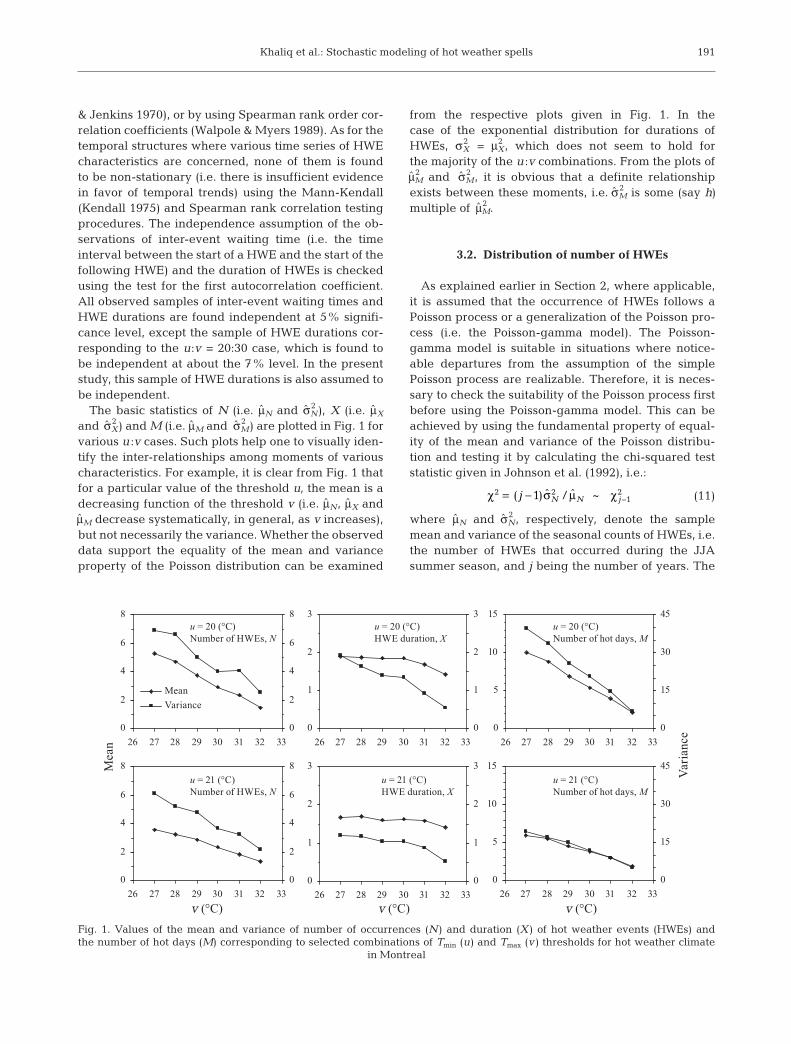
The basic statistics of N (i.e. μN and σ2N), X (i.e. μX

and σ2X) and M (i.e. μM and σ2

M) are plotted in Fig. 1 forvarious u :v cases. Such plots help one to visually iden-tify the inter-relationships among moments of variouscharacteristics. For example, it is clear from Fig. 1 thatfor a particular value of the threshold u, the mean is adecreasing function of the threshold v (i.e. μN, μX andμM decrease systematically, in general, as v increases),but not necessarily the variance. Whether the observeddata support the equality of the mean and varianceproperty of the Poisson distribution can be examined

from the respective plots given in Fig. 1. In thecase of the exponential distribution for durations ofHWEs, σ2

X = μ2X, which does not seem to hold for

the majority of the u :v combinations. From the plots ofμ2

M and σ2M, it is obvious that a definite relationship

exists between these moments, i.e. σ2M is some (say h)

multiple of μ2M.

3.2. Distribution of number of HWEs

As explained earlier in Section 2, where applicable,it is assumed that the occurrence of HWEs follows aPoisson process or a generalization of the Poisson pro-cess (i.e. the Poisson-gamma model). The Poisson-gamma model is suitable in situations where notice-able departures from the assumption of the simplePoisson process are realizable. Therefore, it is neces-sary to check the suitability of the Poisson process firstbefore using the Poisson-gamma model. This can beachieved by using the fundamental property of equal-ity of the mean and variance of the Poisson distribu-tion and testing it by calculating the chi-squared teststatistic given in Johnson et al. (1992), i.e.:

(11)

where μN and σ2N, respectively, denote the sample

mean and variance of the seasonal counts of HWEs, i.e.the number of HWEs that occurred during the JJAsummer season, and j being the number of years. The

χ σ μ χ2 21= −( ) ˆ / ˆj N N j~ –12

191

u = 20 (°C)Number of HWEs, N

u = 20 (°C)HWE duration, X

u = 20 (°C)Number of hot days, M

u = 21 (°C)Number of hot days, M

u = 21 (°C)HWE duration, X

u = 21 (°C)Number of HWEs, N

0

2

4

6

8

26 27 28 29 30 31 32 33

0

2

4

6

8

Mean

Variance

0

1

2

3

26 27 28 29 30 31 32 33

0

1

2

3

0

5

10

15

26 27 28 29 30 31 32 33

0

15

30

45

0

2

4

6

8

26 27 28 29 30 31 32 33

v (°C) v (°C) v (°C)

Mea

n

0

2

4

6

8

0

1

2

3

26 27 28 29 30 31 32 33

0

1

2

3

0

5

10

15

26 27 28 29 30 31 32 33

0

15

30

45

Var

ianc

e

Fig. 1. Values of the mean and variance of number of occurrences (N ) and duration (X ) of hot weather events (HWEs) andthe number of hot days (M) corresponding to selected combinations of Tmin (u) and Tmax (v ) thresholds for hot weather climate

in Montreal

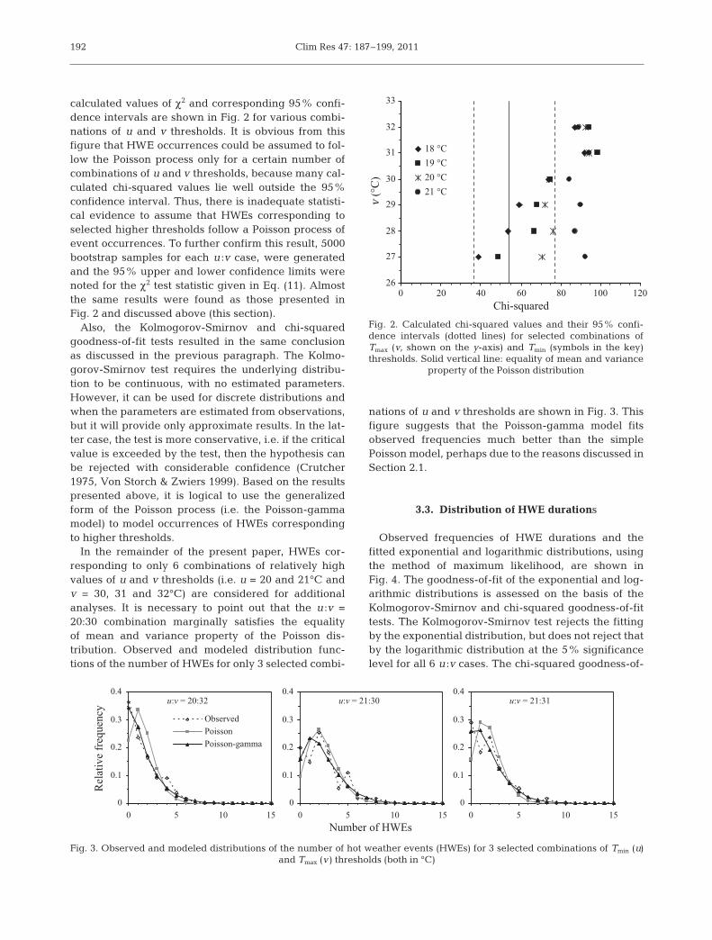
calculated values of χ2 and corresponding 95% confi-dence intervals are shown in Fig. 2 for various combi-nations of u and v thresholds. It is obvious from this figure that HWE occurrences could be assumed to fol-low the Poisson process only for a certain number ofcombinations of u and v thresholds, because many cal-culated chi-squared values lie well outside the 95%confidence interval. Thus, there is inadequate statisti-cal evidence to assume that HWEs corresponding toselected higher thresholds follow a Poisson process ofevent occurrences. To further confirm this result, 5000bootstrap samples for each u :v case, were generatedand the 95% upper and lower confidence limits werenoted for the χ2 test statistic given in Eq. (11). Almostthe same results were found as those presented inFig. 2 and discussed above (this section).

Also, the Kolmogorov-Smirnov and chi-squaredgoodness-of-fit tests resulted in the same conclusionas discussed in the previous paragraph. The Kolmo -gorov-Smirnov test re quires the underlying distribu-tion to be continuous, with no estimated parameters.However, it can be used for discrete distributions andwhen the parameters are estimated from observations,but it will provide only approximate results. In the lat-ter case, the test is more conservative, i.e. if the criticalvalue is exceeded by the test, then the hypothesis canbe rejected with considerable confidence (Crutcher1975, Von Storch & Zwiers 1999). Based on the resultspresented above, it is logical to use the generalizedform of the Poisson process (i.e. the Poisson-gammamodel) to model occurrences of HWEs correspondingto higher thresholds.

In the remainder of the present paper, HWEs cor -responding to only 6 combinations of relatively highvalues of u and v thresholds (i.e. u = 20 and 21°C andv = 30, 31 and 32°C) are considered for additionalanalyses. It is necessary to point out that the u :v =20:30 combination marginally satisfies the equalityof mean and variance property of the Poisson dis -tribution. Observed and modeled distribution func-tions of the number of HWEs for only 3 selected combi-

nations of u and v thresholds are shown in Fig. 3. Thisfigure suggests that the Poisson-gamma model fitsobserved frequencies much better than the simplePoisson model, perhaps due to the reasons discussed inSection 2.1.

3.3. Distribution of HWE durations

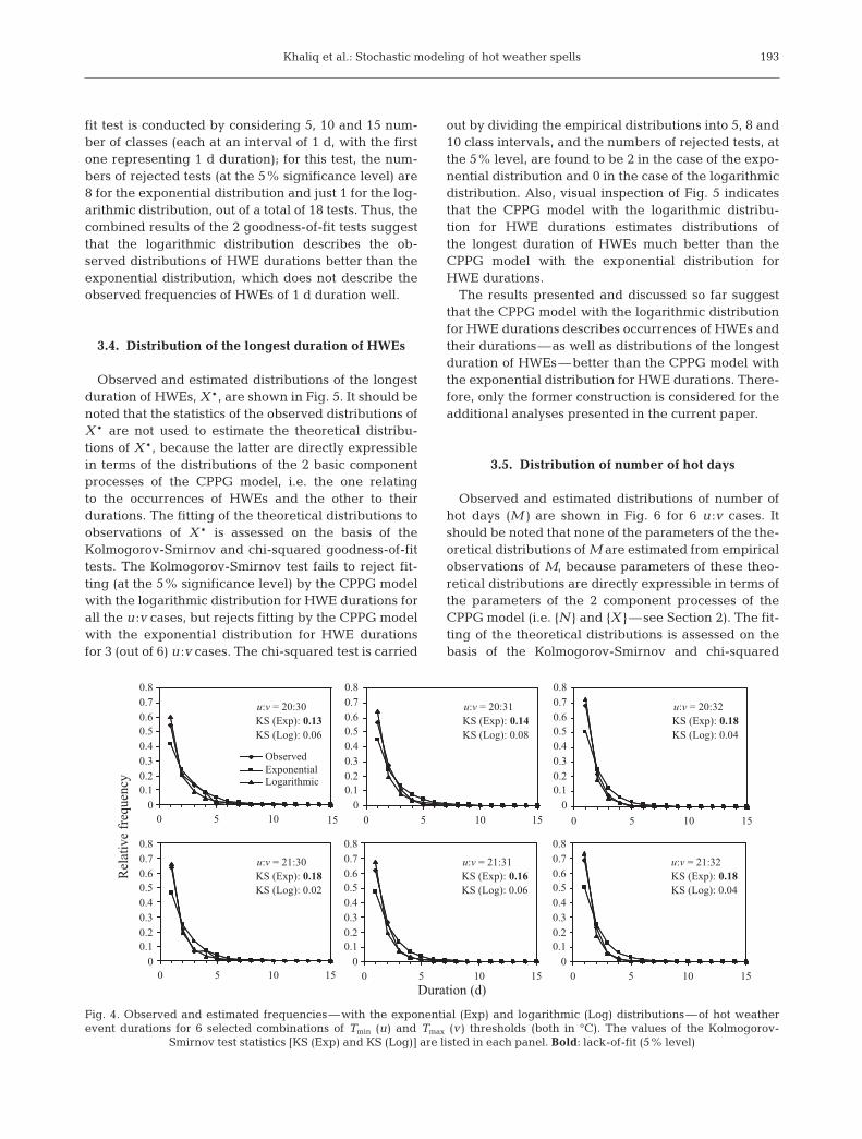
Observed frequencies of HWE durations and the fitted exponential and logarithmic distributions, usingthe method of maximum likelihood, are shown inFig. 4. The goodness-of-fit of the exponential and log-arithmic distributions is assessed on the basis of theKolmogorov-Smirnov and chi-squared goodness-of-fittests. The Kolmogorov-Smirnov test rejects the fittingby the exponential distribution, but does not reject thatby the logarithmic distribution at the 5% significancelevel for all 6 u :v cases. The chi-squared goodness-of-

Clim Res 47: 187–199, 2011192

26

27

28

29

30

31

32

33

0 20 40 60 80 100 120Chi-squared

v (°

C)

18 °C

19 °C

20 °C

21 °C

Fig. 2. Calculated chi-squared values and their 95% confi-dence intervals (dotted lines) for selected combinations ofTmax (v, shown on the y-axis) and Tmin (symbols in the key)thresholds. Solid vertical line: equality of mean and variance

property of the Poisson distribution

u:v = 20:32

0

0.1

0.2

0.3

0.4

0 5 10 15

Rel

ativ

e fr

eque

ncy

ObservedPoissonPoisson-gamma

u:v = 21:30

0

0.1

0.2

0.3

0.4

0 5 10 15

Number of HWEs

u:v = 21:31

0

0.1

0.2

0.3

0.4

0 5 10 15

Fig. 3. Observed and modeled distributions of the number of hot weather events (HWEs) for 3 selected combinations of Tmin (u) and Tmax (v ) thresholds (both in °C)

Khaliq et al.: Stochastic modeling of hot weather spells

fit test is conducted by considering 5, 10 and 15 num-ber of classes (each at an interval of 1 d, with the firstone representing 1 d duration); for this test, the num-bers of rejected tests (at the 5% significance level) are8 for the exponential distribution and just 1 for the log-arithmic distribution, out of a total of 18 tests. Thus, thecombined results of the 2 goodness-of-fit tests suggestthat the logarithmic distribution de scribes the ob -served distributions of HWE durations better than theexponential distribution, which does not describe theobserved frequencies of HWEs of 1 d duration well.

3.4. Distribution of the longest duration of HWEs

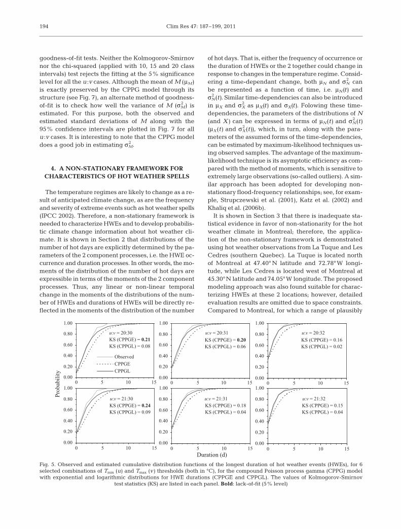
Observed and estimated distributions of the longestduration of HWEs, X*, are shown in Fig. 5. It should benoted that the statistics of the observed distributions ofX* are not used to estimate the theoretical distribu-tions of X*, because the latter are directly expressiblein terms of the distributions of the 2 basic componentprocesses of the CPPG model, i.e. the one relatingto the occurrences of HWEs and the other to their durations. The fitting of the theoretical distributions toobservations of X* is assessed on the basis of the Kolmogorov-Smirnov and chi-squared goodness-of-fittests. The Kolmogorov-Smirnov test fails to reject fit-ting (at the 5% significance level) by the CPPG modelwith the logarithmic distribution for HWE durations forall the u :v cases, but rejects fitting by the CPPG modelwith the exponential distribution for HWE durationsfor 3 (out of 6) u :v cases. The chi-squared test is carried

out by dividing the empirical distributions into 5, 8 and10 class intervals, and the numbers of rejected tests, atthe 5% level, are found to be 2 in the case of the expo-nential distribution and 0 in the case of the logarithmicdistribution. Also, visual inspection of Fig. 5 indicatesthat the CPPG model with the logarithmic distribu -tion for HWE durations estimates distributions ofthe longest duration of HWEs much better than theCPPG model with the exponential distribution forHWE durations.

The results presented and discussed so far suggestthat the CPPG model with the logarithmic distributionfor HWE durations describes occurrences of HWEs andtheir durations—as well as distributions of the longestduration of HWEs—better than the CPPG model withthe exponential distribution for HWE durations. There-fore, only the former construction is considered for theadditional analyses presented in the current paper.

3.5. Distribution of number of hot days

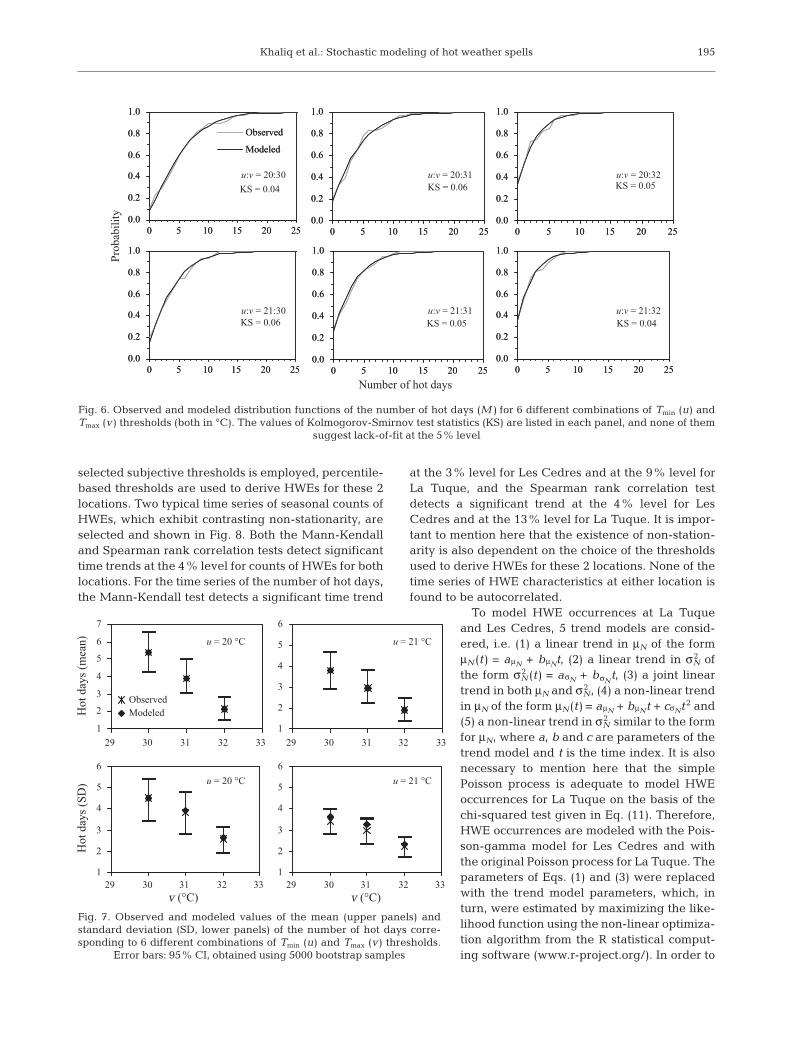
Observed and estimated distributions of number ofhot days (M) are shown in Fig. 6 for 6 u :v cases. Itshould be noted that none of the parameters of the the-oretical distributions of M are estimated from empiricalobservations of M, because parameters of these theo-retical distributions are directly expressible in terms ofthe parameters of the 2 component processes of theCPPG model (i.e. {N } and {X }—see Section 2). The fit-ting of the theo retical distributions is assessed on thebasis of the Kolmogorov-Smirnov and chi-squared

193

KS (Exp): 0.18

KS (Log): 0.02

0 5 10 15

KS (Exp): 0.16

KS (Log): 0.06

0 5 10 15

u:v = 21:32u:v = 21:31u:v = 21:30

u:v = 20:30 u:v = 20:31 u:v = 20:32

KS (Exp): 0.18

KS (Log): 0.04

0 5 10 15

KS (Exp): 0.13

KS (Log): 0.06

0 5 10

ObservedExponentialLogarithmic

KS (Exp): 0.14

KS (Log): 0.08

00.10.20.30.40.50.60.70.8

0 5 10 15

KS (Exp): 0.18

KS (Log): 0.04

0 5 10 15

Duration (d)

15

Rel

ativ

e fr

eque

ncy

00.10.20.30.40.50.60.70.8

00.10.20.30.40.50.60.70.8

00.10.20.30.40.50.60.70.8

00.10.20.30.40.50.60.70.8

00.10.20.30.40.50.60.70.8

Fig. 4. Observed and estimated frequencies—with the exponential (Exp) and logarithmic (Log) distributions—of hot weatherevent durations for 6 selected combinations of Tmin (u) and Tmax (v ) thresholds (both in °C). The values of the Kolmogorov-

Smirnov test statistics [KS (Exp) and KS (Log)] are listed in each panel. Bold: lack-of-fit (5% level)

Clim Res 47: 187–199, 2011

goodness-of-fit tests. Neither the Kolmogorov-Smirnovnor the chi-squared (applied with 10, 15 and 20 classintervals) test rejects the fitting at the 5% significancelevel for all the u :v cases. Although the mean of M (μM)is exactly preserved by the CPPG model through itsstructure (see Fig. 7), an alternate method of goodness-of-fit is to check how well the variance of M (σ2

M) isestimated. For this purpose, both the observed andestimated standard deviations of M along with the95% confidence intervals are plotted in Fig. 7 for allu :v cases. It is interesting to note that the CPPG modeldoes a good job in estimating σ2

M.

4. A NON-STATIONARY FRAMEWORK FORCHARACTERISTICS OF HOT WEATHER SPELLS

The temperature regimes are likely to change as a re-sult of anticipated climate change, as are the frequencyand severity of extreme events such as hot weather spells(IPCC 2002). Therefore, a non-stationary framework isneeded to characterize HWEs and to develop probabilis-tic climate change information about hot weather cli-mate. It is shown in Section 2 that dis tributions of thenumber of hot days are explicitly determined by the pa-rameters of the 2 component processes, i.e. the HWE oc-currence and duration processes. In other words, the mo-ments of the distribution of the number of hot days areexpressible in terms of the moments of the 2 componentprocesses. Thus, any linear or non-linear temporalchange in the moments of the distributions of the num-ber of HWEs and durations of HWEs will be directly re-flected in the moments of the distribution of the number

of hot days. That is, either the frequency of occurrence orthe duration of HWEs or the 2 together could change inresponse to changes in the temperature regime. Consid-ering a time-dependant change, both μN and σ2

N canbe represented as a function of time, i.e. μN(t) andσ2

N(t). Similar time-dependencies can also be introducedin μX and σ2

X as μX(t) and σX(t). Folowing these time- dependencies, the parameters of the distributions of N(and X) can be expressed in terms of μN(t) and σ2

N(t)(μX(t) and σ2

X(t)), which, in turn, along with the para -meters of the assumed forms of the time-dependencies,can be estimated by maximum-likelihood techniques us-ing observed samples. The advantage of the maximum-likelihood technique is its asymptotic efficiency as com -pared with the method of moments, which is sensitive toextremely large observations (so-called outliers). A sim-ilar approach has been adopted for developing non- stationary flood-frequency relationships; see, for exam-ple, Strup czewski et al. (2001), Katz et al. (2002) andKhaliq et al. (2006b).

It is shown in Section 3 that there is inadequate sta-tistical evidence in favor of non-stationarity for the hotweather climate in Montreal; therefore, the applica-tion of the non-stationary framework is demonstratedusing hot weather observations from La Tuque and LesCedres (southern Quebec). La Tuque is located northof Montreal at 47.40° N latitude and 72.78°W longi-tude, while Les Cedres is located west of Montreal at45.30°N latitude and 74.05°W longitude. The proposedmodeling approach was also found suitable for charac-terizing HWEs at these 2 locations; however, detailedevaluation results are omitted due to space constraints.Compared to Montreal, for which a range of plausibly

194

KS (CPPGE) = 0.24

KS (CPPGL) = 0.09

0.00

0.20

0.40

0.60

0.80

1.00

0 5 10 15

KS (CPPGE) = 0.18KS (CPPGL) = 0.04

0.00

0.20

0.40

0.60

0.80

1.00

0 5 10 15Duration (d)

KS (CPPGE) = 0.15KS (CPPGL) = 0.04

0.00

0.20

0.40

0.60

0.80

1.00

0 5 10 15

u:v = 20:30 u:v = 20:31 u:v = 20:32

u:v = 21:30 u:v = 21:31 u:v = 21:32

KS (CPPGE) = 0.21

KS (CPPGL) = 0.08

0.00

0.20

0.40

0.60

0.80

1.00

0 5 10 15

Prob

abili

ty

ObservedCPPGECPPGL

KS (CPPGE) = 0.20

KS (CPPGL) = 0.06

0.00

0.20

0.40

0.60

0.80

1.00

0 5 10 15

KS (CPPGE) = 0.16KS (CPPGL) = 0.02

0.00

0.20

0.40

0.60

0.80

1.00

0 5 10 15

Fig. 5. Observed and estimated cumulative distribution functions of the longest duration of hot weather events (HWEs), for 6 selected combinations of Tmin (u) and Tmax (v ) thresholds (both in °C), for the compound Poisson process gamma (CPPG) modelwith exponential and logarithmic distributions for HWE durations (CPPGE and CPPGL). The values of Kolmo gorov-Smirnov

test statistics (KS) are listed in each panel. Bold: lack-of-fit (5% level)

Khaliq et al.: Stochastic modeling of hot weather spells

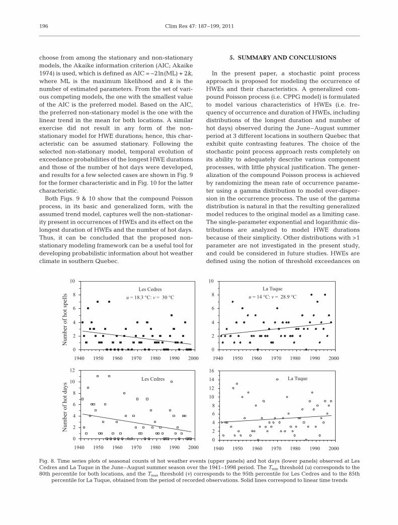
selected subjective thresholds is employed, percentile-based thresholds are used to derive HWEs for these 2locations. Two typical time series of seasonal counts ofHWEs, which exhibit contrasting non-stationarity, areselected and shown in Fig. 8. Both the Mann-Kendalland Spearman rank correlation tests detect significanttime trends at the 4% level for counts of HWEs for bothlocations. For the time series of the number of hot days,the Mann-Kendall test detects a significant time trend

at the 3% level for Les Cedres and at the 9% level forLa Tuque, and the Spearman rank correlation testdetects a significant trend at the 4% level for LesCedres and at the 13% level for La Tuque. It is impor-tant to mention here that the existence of non-station-arity is also dependent on the choice of the thresholdsused to derive HWEs for these 2 locations. None of thetime series of HWE characteristics at either location isfound to be autocorrelated.

To model HWE occurrences at La Tuqueand Les Cedres, 5 trend models are consid-ered, i.e. (1) a linear trend in μN of the formμN (t) = aμN + bμNt, (2) a linear trend in σ2

N ofthe form σ2

N (t) = aσN + bσNt, (3) a joint linear

trend in both μN and σ2N, (4) a non-linear trend

in μN of the form μN(t) = aμN + bμNt + cσNt2 and(5) a non-linear trend in σ2

N similar to the formfor μN, where a, b and c are parameters of thetrend model and t is the time index. It is alsonecessary to mention here that the simplePoisson process is adequate to model HWEoccurrences for La Tuque on the basis of thechi-squared test given in Eq. (11). Therefore,HWE occurrences are modeled with the Pois-son-gamma model for Les Cedres and withthe original Poisson process for La Tuque. Theparameters of Eqs. (1) and (3) were replacedwith the trend model parameters, which, inturn, were estimated by maximizing the like-lihood function using the non-linear optimiza-tion algorithm from the R sta tistical comput-ing software (www.r-project.org/). In order to

195

u:v = 20:30 u:v = 20:31 u:v = 20:32

u:v = 21:30 u:v = 21:31 u:v = 21:32

KS = 0.04

0.0

0.2

0.4

0.6

0.8

1.0

0 5 10 15 20 25

Observed

Modeled

KS = 0.06

0.0

0.2

0.4

0.6

0.8

1.0

0 5 10 15 20 25

KS = 0.05

0.0

0.2

0.4

0.6

0.8

1.0

0 5 10 15 20 25

KS = 0.06

0.0

0.2

0.4

0.6

0.8

1.0

0 5 10 15 20 25

KS = 0.05

0.0

0.2

0.4

0.6

0.8

1.0

0 5 10 15 20 25

Number of hot days

KS = 0.04

0.0

0.2

0.4

0.6

0.8

1.0

0 5 10 15 20 25

0.0

0.2

0.4

0.6

0.8

1.0

0 5 10 15 20 25

Observed

Modeled

0.0

0.2

0.4

0.6

0.8

1.0

0 5 10 15 20 250.0

0.2

0.4

0.6

0.8

1.0

0 5 10 15 20 25

0.0

0.2

0.4

0.6

0.8

1.0

0 5 10 15 20 250.0

0.2

0.4

0.6

0.8

1.0

0 5 10 15 20 250.0

0.2

0.4

0.6

0.8

1.0

0 5 10 15 20 25

Prob

abili

ty

Fig. 6. Observed and modeled distribution functions of the number of hot days (M) for 6 different combinations of Tmin (u) andTmax (v ) thresholds (both in °C). The values of Kolmogorov-Smirnov test statistics (KS) are listed in each panel, and none of them

suggest lack-of-fit at the 5% level

1

2

3

4

5

6

29 30 31 32 33

1

2

3

4

5

6

29 30 31 32 33

u = 20 °C u = 21 °C

u = 20 °C u = 21 °C

1

2

3

4

5

6

7

29 30 31 32 33

ObservedModeled

1

2

3

4

5

6

29 30 31 32 33v (°C) v (°C)

Hot

day

s (m

ean)

Hot

day

s (S

D)

Fig. 7. Observed and modeled values of the mean (upper panels) andstandard deviation (SD, lower panels) of the number of hot days corre-sponding to 6 different combinations of Tmin (u) and Tmax (v ) thresholds.

Error bars: 95% CI, obtained using 5000 bootstrap samples

Clim Res 47: 187–199, 2011

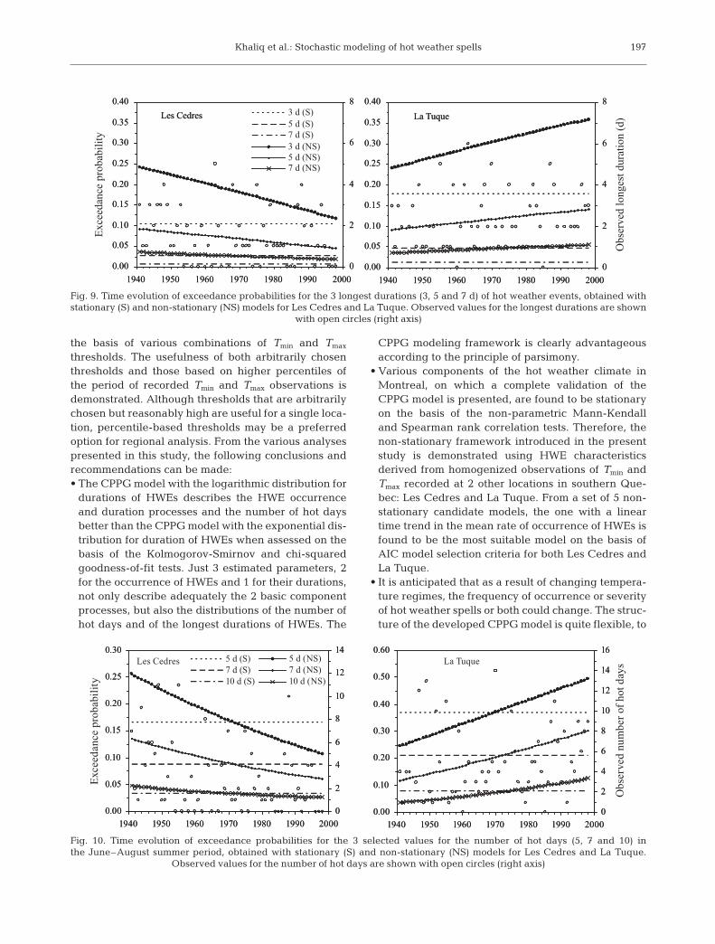
choose from among the stationary and non-stationarymodels, the Akaike information criterion (AIC; Akaike1974) is used, which is defined as AIC = –2ln(ML) + 2k,where ML is the maximum likelihood and k is thenumber of estimated parameters. From the set of vari-ous competing models, the one with the smallest valueof the AIC is the preferred model. Based on the AIC,the preferred non-stationary model is the one with thelinear trend in the mean for both locations. A similarex ercise did not result in any form of the non- stationary model for HWE durations; hence, this char-acteristic can be assumed stationary. Following theselected non-stationary model, temporal evolution ofexceedance probabilities of the longest HWE durationsand those of the number of hot days were developed,and results for a few selected cases are shown in Fig. 9for the former characteristic and in Fig. 10 for the lattercharacteristic.

Both Figs. 9 & 10 show that the compound Poissonprocess, in its basic and generalized form, with theassumed trend model, captures well the non-stationar-ity present in occurrences of HWEs and its effect on thelongest duration of HWEs and the number of hot days.Thus, it can be concluded that the proposed non-stationary modeling framework can be a useful tool fordeveloping probabilistic information about hot weatherclimate in southern Quebec.

5. SUMMARY AND CONCLUSIONS

In the present paper, a stochastic point processapproach is proposed for modeling the occurrence ofHWEs and their characteristics. A generalized com-pound Poisson process (i.e. CPPG model) is formulatedto model various characteristics of HWEs (i.e. fre-quency of occurrence and duration of HWEs, includingdistributions of the longest duration and number ofhot days) observed during the June–August summerperiod at 3 different locations in southern Quebec thatexhibit quite contrasting features. The choice of thestochastic point process approach rests completely onits ability to adequately describe various componentprocesses, with little physical justification. The gener-alization of the compound Poisson process is achievedby randomizing the mean rate of occurrence parame-ter using a gamma distribution to model over-disper-sion in the occurrence process. The use of the gammadistribution is natural in that the resulting generalizedmodel reduces to the original model as a limiting case.The single-parameter exponential and logarithmic dis-tributions are analyzed to model HWE durationsbecause of their simplicity. Other distributions with >1parameter are not investigated in the present study,and could be considered in future studies. HWEs aredefined using the notion of threshold exceedances on

196

Les Cedres

0

2

4

6

8

10

12

1940 1950 1960 1970 1980 1990 2000

Num

ber

of h

ot d

ays

La Tuque

0

2

4

6

8

10

12

14

16

1940 1950 1960 1970 1980 1990 2000

Les Cedres

u = 18.3 °C: v = 30 °C

0

2

4

6

8

10

1940 1950 1960 1970 1980 1990 2000

Num

ber

of h

ot s

pells

La Tuque

u = 14 °C: v = 28.9 °C

0

2

4

6

8

10

1940 1950 1960 1970 1980 1990 2000

Fig. 8. Time series plots of seasonal counts of hot weather events (upper panels) and hot days (lower panels) observed at Les Cedres and La Tuque in the June–August summer season over the 1941–1998 period. The Tmin threshold (u) corresponds to the80th percentile for both locations, and the Tmax threshold (v) corresponds to the 95th percentile for Les Cedres and to the 85th

percentile for La Tuque, obtained from the period of recorded observations. Solid lines correspond to linear time trends

Khaliq et al.: Stochastic modeling of hot weather spells

the basis of various combinations of Tmin and Tmax

thresholds. The usefulness of both arbitrarily chosenthresholds and those based on higher percentiles ofthe period of recorded Tmin and Tmax observations isdemonstrated. Although thresholds that are arbitrarilychosen but reasonably high are useful for a single loca-tion, percentile-based thresholds may be a preferredoption for regional analysis. From the various analysespresented in this study, the following conclusions and recommendations can be made: • The CPPG model with the logarithmic distribution for

durations of HWEs describes the HWE occurrenceand duration processes and the number of hot daysbetter than the CPPG model with the exponential dis-tribution for duration of HWEs when assessed on thebasis of the Kolmogorov-Smirnov and chi-squaredgoodness-of-fit tests. Just 3 estimated parameters, 2for the occurrence of HWEs and 1 for their durations,not only describe adequately the 2 basic componentprocesses, but also the distributions of the number ofhot days and of the longest durations of HWEs. The

CPPG modeling framework is clearly advantageousaccording to the principle of parsimony.

• Various components of the hot weather climate inMontreal, on which a complete validation of theCPPG model is presented, are found to be stationaryon the basis of the non-parametric Mann-Kendalland Spearman rank correlation tests. Therefore, thenon-stationary framework introduced in the presentstudy is demonstrated using HWE characteristicsderived from homogenized observations of Tmin andTmax recorded at 2 other locations in southern Que-bec: Les Cedres and La Tuque. From a set of 5 non-stationary candidate models, the one with a lineartime trend in the mean rate of occurrence of HWEs isfound to be the most suitable model on the basis ofAIC model selection criteria for both Les Cedres andLa Tuque.

• It is anticipated that as a result of changing tempera-ture regimes, the frequency of occurrence or severityof hot weather spells or both could change. The struc-ture of the developed CPPG model is quite flexible, to

197

Les Cedres

0.00

0.05

0.10

0.15

0.20

0.25

0.30

0.35

0.40

1940 1950 1960 1970 1980 1990 2000

0

2

4

6

8

5 d (S)7 d (S)3 d (NS)5 d (NS)7 d (NS)

La Tuque

0.00

0.05

0.10

0.15

0.20

0.25

0.30

0.35

0.40

1940 1950 1960 1970 1980 1990 2000

0

2

4

6

8

Les Cedres

0.00

0.05

0.10

0.15

0.20

0.25

0.30

0.35

0.40

1940 1950 1960 1970 1980 1990 2000

0

2

4

6

83 d (S) La Tuque

0.00

0.05

0.10

0.15

0.20

0.25

0.30

0.35

0.40

1940 1950 1960 1970 1980 1990 2000

0

2

4

6

8E

xcee

danc

e pr

obab

ility

Obs

erve

d lo

nges

t dur

atio

n (d

)

Fig. 9. Time evolution of exceedance probabilities for the 3 longest durations (3, 5 and 7 d) of hot weather events, obtained withstationary (S) and non-stationary (NS) models for Les Cedres and La Tuque. Observed values for the longest durations are shown

with open circles (right axis)

Les Cedres

0.00

0.05

0.10

0.15

0.20

0.25

0.30

1940 1950 1960 1970 1980 1990 20000

2

4

6

8

10

12

145 d (S)7 d (S)10 d (S)

5 d (NS)7 d (NS)10 d (NS)

La Tuque

0.00

0.10

0.20

0.30

0.40

0.50

0.60

1940 1950 1960 1970 1980 1990 20000

2

4

6

8

10

12

14

16

0.00

0.05

0.10

0.15

0.20

0.25

0.30

1940 1950 1960 1970 1980 1990 20000

2

4

6

8

10

12

14

0.00

0.10

0.20

0.30

0.40

0.50

0.60

1940 1950 1960 1970 1980 1990 20000

2

4

6

8

10

12

14

16

Exc

eeda

nce

prob

abil

ity

Obs

erve

d nu

mbe

r of

hot

day

s

Fig. 10. Time evolution of exceedance probabilities for the 3 selected values for the number of hot days (5, 7 and 10) inthe June–August summer period, obtained with stationary (S) and non-stationary (NS) models for Les Cedres and La Tuque.

Observed values for the number of hot days are shown with open circles (right axis)

Clim Res 47: 187–199, 2011

accommodate both of these aspects in terms of time-dependent model parameters; hence, it could be auseful tool for developing probabilistic informationabout the behavior of hot weather spells for a smalleror larger spatial domain.

• Occurrence of HWEs is a regional mechanism. There -fore, small homogeneous regions based on somephys ical factors or purely based on statisticalapproaches (see, for example, Hosking & Wallis1997) could be defined, and regional averaged timeseries of the 2 component processes of the CPPGmodel could be derived for a regional analysis.Future studies could consider this extension of themodel. Furthermore, the non-stationary frameworkproposed is quite general. It could be extended fur-ther by including indices of large-scale atmosphericcirculations in the parameters of the distributions ofthe number of HWEs or durations of HWEs as co -variates. This will help develop non-stationary and/ornon-identical frequency analysis procedures in asimilar manner as for other hydrometeorological vari-ables (see, for example, Katz et al. 2002, Khaliq etal. 2006b).

• The intensity aspect of HWEs is taken into con -sideration by using various thresholds with increas-ing magnitudes. However, if the interest lies in modeling magnitudes of exceedances, then that canbe achieved by extending the univariate approach(described in Katsoulis & Hatzianastassiou 2005 andFurrer et al. 2010) to a multivariate setting, in orderto model exceedances of both daily minimum andmaximum temperature thresholds. Compared to theintensity aspect, modeling seasonality of hot weatherspells over the summer season is a challenging task.One possible solution would be to concentrate sepa-rately on small seasonal time windows.

Acknowledgements. The financial support provided by theOuranos Consortium on Regional Climatology and Adapta-tion to Climate Change, during 2005–2006, is gratefullyacknowledged. The access to Environment Canada homoge-nized temperature dataset is fully appreciated. We are thank-ful to 3 anonymous referees for their valuable comments thatled to an improved article, and to Prof. André St-Hilaire forreviewing an earlier version of the paper.

LITERATURE CITED

Abaurrea J, Cebrián AC (2002) Drought analysis based on acluster Poisson model: distribution of the most severedrought. Clim Res 22:227–235

Abramowitz M, Stegun IA (1965) Handbook of mathematicalfunctions with formulas, graphs and mathematical tables.Dover Publications, New York

Akaike H (1974) A new look at the statistical model identifica-tion. IEEE Trans Automat Contr 19:716–722

Anderson RL (1942) Distribution of the serial correlation coef-ficient. Ann Math Stat 13:1–13

Box GEP, Jenkins GM (1970) Time series analysis: forecastingand control. Holden-Day, San Francisco, CA

Cameron AC, Trivedi PK (1998) Regression analysis of countdata. Cambridge University Press, Cambridge

Cox DR, Isham V (1980) Point processes. Chapman & Hall,London

Crutcher HL (1975) A note of the possible misuse of the Kolmogorov-Smirnov test. J Appl Meteorol 14:1600–1603

Elsner JB, Bossak BH (2001) Bayesian analysis of US hurri-cane climate. J Clim 14:4341–4350

Feller RW (1968) An introduction to probability theory and itsapplications, Vol 1. John Wiley, New York

Furrer EM, Katz RW, Walter MD, Furrer R (2010) Statisticalmodeling of hot spells and heat waves. Clim Res 43:191–205

Guttorp P (1995) Stochastic modeling of scientific data. Chap-man & Hall, London

Hosking JRM, Wallis JR (1997) Regional frequency analysis.Cambridge University Press, Cambridge

IPCC (Intergovernmental Panel on Climate Change) (2002)IPCC workshop report on ‘changes in extreme weather andclimate events’, Beijing, China, 11-13 June, 2002. Availableat www.ipcc.ch/publications_and_data/publications _ and_data_supporting_material.shtml (accessed on 14 September2010)

Johnson NL, Kotz S, Kemp AW (1992) Univariate discrete distributions. John Wiley, New York

Katsoulis BD, Hatzianastassiou N (2005) Analysis of hot spellcharacteristics in the Greek region. Clim Res 28:229–241

Katz RW (2002) Stochastic modeling of hurricane damage.J Appl Meteorol 41:754–762

Katz RW, Parlange MB, Naveau P (2002) Statistics of extremesin hydrology. Adv Water Resour 25:1287–1304

Kendall MG (1975) Rank correlation methods. Charless Griffin, London

Kendall MG, Stuart A (1977) The advanced theory of statis-tics, Vol 1. Charless Griffin & Company, London

Khaliq MN, St-Holaire A, Ouarda TBMJ, Bobée B (2005) Fre-quency analysis and temporal pattern of occurrences ofsouthern Quebec heatwaves. Int J Climatol 25:485–504

Khaliq MN, Gachon P, St-Hilaire A, Ouarda TBMJ, Bobée B(2006a) Southern Quebec (Canada) summer-season heatspells over the 1941–2000 period: an assessment of ob -served changes. Theor Appl Climatol 88:83–101

Khaliq MN, Ouarda TBMJ, Ondo JC, Gachon P, Bobée B(2006b) Frequency analysis of a sequence of dependentand/or non-stationary hydro-meteorological observations:a review. J Hydrol (Amst) 329:534–552

Khaliq MN, Ouarda TBMJ, St-Hilaire A, Gachon P (2007)Bayesian change-point analysis of heatspell occurrencesin Montreal, Canada. Int J Climatol 27:807–818

Medhi J (2002) Stochastic processes. New Age International,New Delhi

Parzen E (1964) Stochastic processes. Holden-Day, San Francisco, CA

Prieto L, Herrera RG, Díaz J, Hernández E, del Teso T (2004)Minimum extreme temperatures over Peninsular Spain.Global Planet Change 44:59–71

Reiss RD, Thomas M (2007) Statistical analysis of extreme values. Birkhäuser Verlag, Basel

Rodriguez-Iturbe I, Cox DR, Isham V (1987) Some models forrainfall based on stochastic point processes. Proc R SocLond A 410:269–288

Rootzén H, Tajvidi N (1997) Extreme value statistics and windstorm losses: a case study. Scand Actuar J 1997:70–94

Skinner CJ (1992) On identification disclosure and predictiondisclosure for micro data. Stat Neerl 46:21–32

198

Khaliq et al.: Stochastic modeling of hot weather spells 199

Snedecor G, Cochran WG (1980) Statistical methods. TheIowa State University Press, Ames

Strupczewski WG, Singh VP, Mitosek HT (2001) Non-stationary approach to at-site flood frequency modeling.III. Flood analysis of Polish rivers. J Hydrol (Amst) 248:152–167

Vincent LA, Zhang X, Bonsal BR, Hogg WD (2000) Homoge-nized daily temperatures for trend analyses in extremesover Canada. In: Preprint 12th Conf Applied Climatology.Ashville, NC, AM Meteorol Soc p 86–89

Vincent LA, Zhang X, Bonsal BR, Hogg WD (2002) Homo -genization of daily temperatures over Canada. J Clim 15:1322–1334

Von Storch H, Zwiers FW (1999) Statistical analysis in climateresearch. Cambridge University Press, Cambridge

Walpole RE, Myers RH (1989) Probability and statistics forengineers and scientists. Macmillan Publishing Company,New York

Zelenhasic E, Salvai A (1987) A method of streamflowdrought analysis. Water Resour Res 23:156–168

Appendix 1. Distribution function of the number of hot days for the compound Poisson process model

If X is assumed to follow the discrete logarithmic distribu-tion then the conditional probability P (M = m |N = n) can bederived from the probability generating function (pgf) of X,which is given by Kendall & Stuart (1977, p. 139) as:

(A1)

Given N = n, the conditional distribution of M is the sum ofn independent random variables. The pgf of M is the n-foldconvolution of G(s), i.e.:

(A2)

Using the standard theorems of combinatorial mathematics(Abramowitz & Stegun 1965, p. 824), the second term onthe right-hand side of Eq. (A2) can be transformed in termsof Stirling’s numbers of first kind, i.e. the pgf of M can be

written as:

(A3)

where SNF nj is the Stirling’s number of the first kind. In the

expansion of the pgf, Eq. (A3), as a power series in s, theP (M = m |N = n) is given by the coefficient of s j (see Medhi2002, p. 7). Thus:

(A4)

After some algebraic manipulations, the unconditionalprobability, P (M = n), in the case of the basic compoundPoisson process, i.e. when Eq. (1) is applicable, and in thecase of the CPPG model can be derived from Eq. (A4). Cor-responding expressions are provided in Eqs. (9) and (10),respectively, in the main article.

G s E sbs

aX( )

log( )log

= = −[ ]

1

G sa

bsnn

n( )(log )

log( )[ ] = −[ ]11

G sn

aSNF

bsj

n

nj

jn

j n

j

( )!

(log )( )

( )!

[ ] = −=

∞

∑ 1

P M m N nb n

a mSNFm

m

n mn( ) ( )

!(log ) !

= = = −| 1

Editorial responsibility: Helmut Mayer, Freiburg, Germany

Submitted: September 22, 2010; Accepted: March 29, 2011Proofs received from author(s): June 28, 2011