Stochastic Knowledge Representations and Machine

Learning Strategies for Biological Sequence Analysis

Hiroshi Mamitsuka

Abstract

We establish novel stochastic knowledge representations and new machine learning strategies tosolve four important problems in the field of molecular biology. In particular, we focus on the problemof predicting protein structures, e.g. α-helices, β-sheets and typical structural motifs, which has beenregarded as a principal theme in this field.

A common feature of the four methods is that each builds a stochastic model to represent thetarget objective in the respective problem setting, and the methods are expected to be robust againsterrors or noise which are liable to occur in biological databases obtained through rather manual andcomplicated biochemical experiments. It should be emphasized that our algorithms for training eachof the stochastic models from given examples have a sufficient degree of originality (particularly interms of computer science) relative to conventional algorithms for each of the problems involved, andthat we evaluate our methods in computational experiments and in the experiments performed, morefavorable performance can be obtained with them than with other existing algorithms.

Following a brief introduction, this thesis begins in Chapter 2 by introducing the problems inmolecular biology and the techniques of machine learning that are dealt with in this thesis. Specifically,we concentrate on the problem of predicting protein structures in detail. We emphasize that all of ourlearning methods are based on the minimum description length (MDL) principle, the use of which isdescribed in Chapters 3 and 4, and on maximum likelihood estimation which is the basis of all thealgorithms outside of MDL learning described in this thesis.

In Chapter 3, we address the problem of predicting protein α-helix regions, which are one ofthe major secondary structures and is believed to be formed from its local properties. For thisproblem, we define a stochastic rule with finite partitioning to represent an amino acid distributionat each residue position in an α-helix. We then establish a strategy based on the MDL principle tooptimize the structure of the stochastic rule. In other words, we obtain optimal clustering of aminoacid types at a position. To make the optimization possible, we use the sequences whose three-dimensional structures are unknown, to enhance the amount of available data and greatly improvethe prediction accuracy of our method. Among the experiments we conducted was a large-scale oneinvolving data on more than five thousand amino acids, and the results obtained show that the methodwe developed achieved 81% prediction accuracy. This exceeded the 75% accuracy obtained with Qianand Sejnowski’s (QS) method for the same data and was on the same level as the results obtainedwith Rost and Sander’s (RS) method which was widely considered to be the best secondary structureprediction method. One of the merits of our method is that it can provide comprehensible rules ofα-helices while QS and RS cannot.

In Chapter 4, we propose a new method for representing inter-residue relations in motifs, whichare structural or functional key portions hidden in amino acid sequences. We define a probabilisticnetwork with finite partitionings in which an arc represents an inter-residue relation between nodescorresponding to residue positions. Based on the MDL principle and a greedy-search from givenexamples, we establish an efficient learning algorithm which automatically constructs a near-optimalprobabilistic network. Our experiments using an actual protein motif show that our method built aprobabilistic network with finite partitionings, in which each inter-residue relation corresponded toan actual bio-chemical feature peculiar to the motif. Moreover, this network, which provides visibleinter-residue relations, had the same level of motif classification accuracy as a feed-forward type neuralnetwork trained by an ordinary learning approach, which network however cannot provide any visibleinformation.

In Chapter 5, we propose a new method for learning a hidden Markov model, which have beenused as a model for representing multiple aligned sequences of a certain functional or structural

i

class. The conventional algorithm of hidden Markov models, called the Baum-Welch algorithm, hasthe disadvantage of not always being able to provide sufficient discrimination ability because thealgorithm uses only the sequences belonging to the class of interest, and not those that do not. Onthe other hand, we establish a new efficient learning algorithm which uses not only the sequencesbelonging to the class, but also sequences that do not, called negative examples. This allows us toenhance the discrimination ability of the Baum-Welch algorithm. Furthermore, with our algorithm,hidden Markov models can be applied to data in which each example has a label. In other words, ourmethod realizes a supervised learning of hidden Markov models. In our experiments, we used actualamino acid sequences consisting of both positive and negative examples of an existing motif in orderto evaluate the discrimination ability of our method and of three other existing methods includingthe Baum-Welch algorithm. Experimental results show that for the dataset in question, our methodgreatly reduced discrimination errors as compared to the other two methods.

In Chapter 6, we propose a new method for the problem of predicting the location of β-sheets,which along with α-helices, are one of the major secondary structures. The difficulty of this problem isthat the dependencies of β-strands forming a β-sheet in the amino-acid sequence are unbounded. Tocope with this difficulty, we define a new family of stochastic tree grammars which we call a stochasticranked node rewriting grammar, which is powerful enough to capture such unbounded dependencies.Furthermore, we establish a new learning algorithm for the tree grammars, and add a number ofsignificant modifications to the grammars and the algorithm. In our experiments, we conducted anumber of experiments with data in which no test sequence has more than 25% pairwise sequencesimilarity to any training protein. Experimental results show that our method captured the longdistance dependency in β-sheet regions, thus providing positive evidence for the potential of ourmethod as a tool for scientific discovery that allows us to discover unnoticed structural similarity inproteins having no or little sequence similarity.

In Chapter 7, we give concluding remarks and mention some possible future work related toenhance the performance of our current methods.

ii

Acknowledgments

The author would like to express his deepest gratitude to his thesis supervisor Prof. Satoru Miyano ofthe University of Tokyo for his valuable guidance and advice, which was greatly helpful in completingthis thesis. The author would also like to thank the members of his thesis commitee: Prof. KentaroShimizu, Prof. Hiroshi Imai and Prof. Tatsuya Akutsu of the University of Tokyo and Prof. TomoyukiHiguchi of the Institute of Statistical Mathematics for their valuable comments and suggestions.

The author would like to express his sincere gratitude to Dr. Naoki Abe and Dr. Kenji Yamanishiof C&C Media Research Laboratories, NEC Corporation. They have offered a number of adviceand suggestions since he joined NEC Corporation, and their early guidance instilled in the authorconfidence in his research ability. Chapters 3 and 6 of this thesis are fruitful results produced by jointwork with them.

The author also thanks Prof. Akihiko Konagaya of JAIST. It is Prof. Konagaya who first intro-duced the author to the field of computational biology (or genetic information processing), while hewas with NEC Corporation.

The research described in this thesis was conducted at C&C Media Research Labs, NEC Cor-poration. The author thanks Atsuyoshi Nakamura, Li Hang and Jun-ichi Takeuchi of the “MachineLearning” group of C&C Media Research Labs, NEC Corpotation for their helpful advice and sug-gestions. The author also thanks Mr. Katsuhiro Nakamura, Mr. Tomoyuki Fujita and Dr. Shun Doiof NEC Corporation for their constant support and encouragement.

Special thanks also go to Dr. Ken-ichi Takada of NIS, who implemented the parallel parsingalgorithm of stochastic tree grammars in Chapter 6.

iii

Publication Notes

Chapter 3 is based on three papers which appeared in the journal Computer Applications in theBiosciences (Mamitsuka & Yamanishi, 1995), in the proceedings of the 26th Hawaii InternationalConference on System Sciences (Mamitsuka & Yamanishi, 1993) and in the proceedings of the ThirdWorkshop on Algorithmic Learning Theory (Mamitsuka & Yamanishi, 1992). All of these representjoint work participated in by Dr. Kenji Yamanishi of NEC Corporation.

Chapter 4 is based on two papers which appeared in the journal Computer Applications in theBiosciences (Mamitsuka, 1995) and appeared in the proceedings of Genome Informatics WorkshopIV (Mamitsuka, 1993).

Chapter 5 is based on three papers which appeared in the Journal of Computational Biology(Mamitsuka, 1996) , in the journal Proteins: Structure, Function and Genetics (Mamitsuka, 1998)and in the proceedings of the First International Conference on Computational Molecular Biology(Mamitsuka, 1997).

Chapter 6 is based on five papers which appeared in the journal Machine Learning (Abe & Mamit-suka, 1997), in the proceedings of the 11th International Conference on Machine Learning (Abe &Mamitsuka, 1994), in the proceedings of the Second International Conference on Intelligent Systemsfor Molecular Biology (Mamitsuka & Abe, 1994a), in the proceedings of Genome Informatics Work-shop V (Mamitsuka & Abe, 1994b) and in the proceedings of the 15th International Conference onMachine Learning (Abe & Mamitsuka, 1998). All of these represent joint work participated in by Dr.Naoki Abe of NEC Corporation.

iv

Contents

1 Introduction 1

2 Problems in Molecular Biology and Machine Learning 92.1 Computational Problems in Molecular Biology . . . . . . . . . . . . . . . . . . . . . . 9

2.1.1 Fundamentals of Molecular Biology . . . . . . . . . . . . . . . . . . . . . . . . . 102.1.2 Protein Structure Prediction . . . . . . . . . . . . . . . . . . . . . . . . . . . . 152.1.3 Multiple Sequence Alignment - Profile Calculation . . . . . . . . . . . . . . . . 192.1.4 Motif Detection / Discrimination / Classification . . . . . . . . . . . . . . . . . 21

2.2 Machine Learning . . . . . . . . . . . . . . . . . . . . . . . . . . . . . . . . . . . . . . . 222.2.1 Fundamentals of Machine Learning . . . . . . . . . . . . . . . . . . . . . . . . . 222.2.2 Model Classes . . . . . . . . . . . . . . . . . . . . . . . . . . . . . . . . . . . . . 232.2.3 Learning Algorithms . . . . . . . . . . . . . . . . . . . . . . . . . . . . . . . . . 32

3 Predicting α-helices Based on Stochastic Rule Learning 403.1 Introduction . . . . . . . . . . . . . . . . . . . . . . . . . . . . . . . . . . . . . . . . . . 403.2 Stochastic Rule Learning Method . . . . . . . . . . . . . . . . . . . . . . . . . . . . . . 43

3.2.1 Example Generation . . . . . . . . . . . . . . . . . . . . . . . . . . . . . . . . . 433.2.2 Learning Phase . . . . . . . . . . . . . . . . . . . . . . . . . . . . . . . . . . . . 463.2.3 Prediction Phase . . . . . . . . . . . . . . . . . . . . . . . . . . . . . . . . . . . 49

3.3 Experimental Results . . . . . . . . . . . . . . . . . . . . . . . . . . . . . . . . . . . . . 513.3.1 Performance Measure . . . . . . . . . . . . . . . . . . . . . . . . . . . . . . . . 513.3.2 Stochastic Rule Learning Method . . . . . . . . . . . . . . . . . . . . . . . . . . 523.3.3 Neural Network Learning Method . . . . . . . . . . . . . . . . . . . . . . . . . 53

3.4 Conclusion . . . . . . . . . . . . . . . . . . . . . . . . . . . . . . . . . . . . . . . . . . 57

4 Representing Inter-residue Relations with Probabilistic Networks 594.1 Introduction . . . . . . . . . . . . . . . . . . . . . . . . . . . . . . . . . . . . . . . . . . 594.2 Method . . . . . . . . . . . . . . . . . . . . . . . . . . . . . . . . . . . . . . . . . . . . 61

4.2.1 Probabilistic Network with Finite Partitionings . . . . . . . . . . . . . . . . . . 614.2.2 Efficient MDL Learning Algorithm for Probabilistic Networks . . . . . . . . . . 61

4.3 Experimental Results . . . . . . . . . . . . . . . . . . . . . . . . . . . . . . . . . . . . . 644.3.1 Data – EF-hand Motif . . . . . . . . . . . . . . . . . . . . . . . . . . . . . . . . 644.3.2 Training Probabilistic Network with Finite Partitionings . . . . . . . . . . . . . 654.3.3 Comparing Probabilistic Network with Neural Network in Cross-validation Test 69

4.4 Conclusion . . . . . . . . . . . . . . . . . . . . . . . . . . . . . . . . . . . . . . . . . . 71

v

5 Supervised Learning of Hidden Markov Models 725.1 Introduction . . . . . . . . . . . . . . . . . . . . . . . . . . . . . . . . . . . . . . . . . . 725.2 Hidden Markov Models . . . . . . . . . . . . . . . . . . . . . . . . . . . . . . . . . . . 745.3 Supervised Learning Algorithm for Hidden Markov Models . . . . . . . . . . . . . . . 755.4 Experimental Results – 1 . . . . . . . . . . . . . . . . . . . . . . . . . . . . . . . . . . 78

5.4.1 Data – Lipocalin Family Motif . . . . . . . . . . . . . . . . . . . . . . . . . . . 785.4.2 Comparing Supervised Learning Method with Other Methods in Cross-validation

Test . . . . . . . . . . . . . . . . . . . . . . . . . . . . . . . . . . . . . . . . . . 795.5 Experimental Results – 2 . . . . . . . . . . . . . . . . . . . . . . . . . . . . . . . . . . 83

5.5.1 Data – MHC Binding Peptides . . . . . . . . . . . . . . . . . . . . . . . . . . . 845.5.2 Comparing Supervised Learning Method with Other Methods in Cross-validation

Test . . . . . . . . . . . . . . . . . . . . . . . . . . . . . . . . . . . . . . . . . . 855.5.3 Predicting Peptides That Bind to MHC Molecule . . . . . . . . . . . . . . . . . 87

5.6 Conclusion . . . . . . . . . . . . . . . . . . . . . . . . . . . . . . . . . . . . . . . . . . 90

6 Discovering Common β-sheets with Stochastic Tree Grammar Learning 926.1 Introduction . . . . . . . . . . . . . . . . . . . . . . . . . . . . . . . . . . . . . . . . . . 926.2 Stochastic Tree Grammars and β-Sheet Structures . . . . . . . . . . . . . . . . . . . . 95

6.2.1 Stochastic Ranked Node Rewriting Grammars (SRNRGs) . . . . . . . . . . . . 956.2.2 Modeling β-Sheet Structures with RNRG . . . . . . . . . . . . . . . . . . . . . 98

6.3 Learning and Parsing of Restricted Subclass . . . . . . . . . . . . . . . . . . . . . . . . 996.3.1 Learning Algorithm for Linear SRNRG . . . . . . . . . . . . . . . . . . . . . . 1016.3.2 Reducing Alphabet Size with MDL Approximation . . . . . . . . . . . . . . . . 1046.3.3 Parallel Parsing Algorithm and Prediction . . . . . . . . . . . . . . . . . . . . . 105

6.4 Experimental Results . . . . . . . . . . . . . . . . . . . . . . . . . . . . . . . . . . . . . 1086.4.1 Cross-prediction with Structurally Similar Proteins . . . . . . . . . . . . . . . . 1086.4.2 Capturing Correlations with Multiple Rewriting Rules . . . . . . . . . . . . . . 1096.4.3 Towards Scientific Discovery . . . . . . . . . . . . . . . . . . . . . . . . . . . . 111

6.5 Conclusion . . . . . . . . . . . . . . . . . . . . . . . . . . . . . . . . . . . . . . . . . . 118

7 Concluding Remarks and Future Perspective 1197.1 Summary . . . . . . . . . . . . . . . . . . . . . . . . . . . . . . . . . . . . . . . . . . . 1197.2 Future Directions . . . . . . . . . . . . . . . . . . . . . . . . . . . . . . . . . . . . . . . 120

Bibliography 122

vi

Chapter 1

Introduction

Computational Needs in Molecular Biology

A number of world-wide genome sequencing projects for various types of living organisms includinghuman beings have been promoted over the world since the early 1990s. With the advent of recentnewly developed technologies in genetic engineering, these projects have rapidly accumulated an enor-mous amount of genetic sequence data for some living organisms, e.g. Arabidopsis thaliana (Meinkeet al., 1998) and Caenorhabditis elegans (The C.elegans consortium, 1998), during the last these fewyears. Surprisingly, one report (Pennisi, 1999) predicts that most of the entire human genome, whichcorresponds to twenty-three human chromosome pairs, i.e. nearly three billion bases, will be sequencedat an accuracy of 99% by the spring of 2000. This is considerably earlier than the initial target dateof 2005 which had previously estimated. This amount of information on the human genome, corre-sponding to 750 megabytes of digital information (Olson, 1995), is said to be equal to the amount ofinformation printed in a major newspaper over a period of almost twenty years.

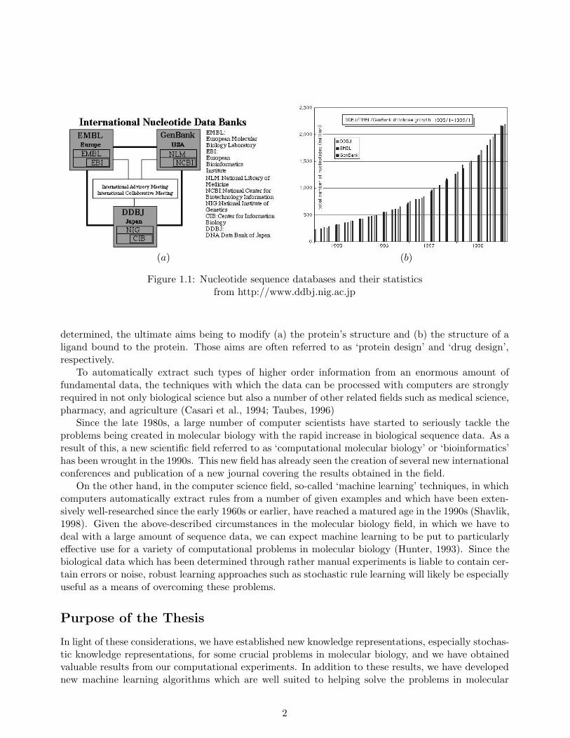
Actually, sequence databases to which newly sequenced genetic data submitted have taken a quan-tum leap in size these last few years. To date, there exist three major nucleotide sequence databases,i.e. DDBJ (DNA Data Bank of Japan) (Sugawara, Miyazaki, Gojobori, & Tateno, 1999), Gen-Bank (Benson, Boguski, Lipman, Ostell, Ouelette, Rapp, & Wheeler, 1999), and EMBL (EuropeanMolecular Biology Laboratory Nucleotide Sequence Databank) (Stoesser, Tuli, Lopez, & Sterk, 1999)in Japan, USA and Europe, respectively, which databases complement each other as shown in Figure1.1 (a). Figure 1.1 (b) which shows the accumulated number of nucleotides in these databases dur-ing the past few years, indicates that for all three, the number of annual nucleotides has drasticallyincreased every year and that the total number of nucleotides surpassed twenty billion in 1998. Ac-cording to the DDBJ, the total number of the nucleotides in these databases may be in one hundred ofbillions in the near future, given the accelerating pace at which sequencing data is being accumulated.

The genetic sequence data being determined or which will be determined in this way includesinformation not only on each component in living organisms but also information regarding the timingwith which components are produced from their genes, and even information about the interactivefunctions between the components, and thus we can say that the sequence information is a compressedcipher to explicate all living phenomena in this world. In other words, we can say that the sequencedata is the most fundamental information in molecular biology.

Under these circumstances, to elucidate a variety of living phenomena and further to regulatethem, we need to extract higher order information from the accumulated fundamental information inmolecular biology. A typical example of extracting higher order information from the sequence data isto predict the 3-dimensional structure of a protein whose fundamental information has already been

1

(a) (b)

Figure 1.1: Nucleotide sequence databases and their statisticsfrom http://www.ddbj.nig.ac.jp

determined, the ultimate aims being to modify (a) the protein’s structure and (b) the structure of aligand bound to the protein. Those aims are often referred to as ‘protein design’ and ‘drug design’,respectively.

To automatically extract such types of higher order information from an enormous amount offundamental data, the techniques with which the data can be processed with computers are stronglyrequired in not only biological science but also a number of other related fields such as medical science,pharmacy, and agriculture (Casari et al., 1994; Taubes, 1996)

Since the late 1980s, a large number of computer scientists have started to seriously tackle theproblems being created in molecular biology with the rapid increase in biological sequence data. As aresult of this, a new scientific field referred to as ‘computational molecular biology’ or ‘bioinformatics’has been wrought in the 1990s. This new field has already seen the creation of several new internationalconferences and publication of a new journal covering the results obtained in the field.

On the other hand, in the computer science field, so-called ‘machine learning’ techniques, in whichcomputers automatically extract rules from a number of given examples and which have been exten-sively well-researched since the early 1960s or earlier, have reached a matured age in the 1990s (Shavlik,1998). Given the above-described circumstances in the molecular biology field, in which we have todeal with a large amount of sequence data, we can expect machine learning to be put to particularlyeffective use for a variety of computational problems in molecular biology (Hunter, 1993). Since thebiological data which has been determined through rather manual experiments is liable to contain cer-tain errors or noise, robust learning approaches such as stochastic rule learning will likely be especiallyuseful as a means of overcoming these problems.

Purpose of the Thesis

In light of these considerations, we have established new knowledge representations, especially stochas-tic knowledge representations, for some crucial problems in molecular biology, and we have obtainedvaluable results from our computational experiments. In addition to these results, we have developednew machine learning algorithms which are well suited to helping solve the problems in molecular

2

biology.We here note that the strategies which we will propose in this thesis are strongly related to pre-

dicting protein structures, since the protein structure prediction problem is the single most importantproblem in the molecular biology field with its broad scientific and engineering applications. Exist-ing approaches proposed to solve the problem have been far from satisfactory to solve for molecularbiologists though a number of attempts have been made on the problem through the use of computers.

In the thesis, Chapters 3 and 6 deal with predicting protein secondary structures (α-helix andβ-sheet, respectively) which are regularly and frequently seen in protein 3-dimensional structures.The α-helix prediction method based on stochastic rule learning, which is proposed in Chapter 3,achieved residue-wise prediction accuracy of over 80%, which was almost the same level as that ofPHD (Profile network from HeiDelberg) (Rost, Sander, & Schneider, 1994) which had been the mostpowerful prediction method available. The β-sheet prediction method using stochastic tree-grammarlearning, which is proposed in Chapter 6, provides a complete new approach toward representingβ-sheet structures, which has not been tried yet in any secondary structure prediction method or inany 3-dimensional prediction method.

The main purpose of this thesis is to establish novel stochastic knowledge representations andmachine learning strategies for the crucial problems in biological sequence analysis, and to demonstratein terms of computational experiments that our methods including two ones described above, areeffective means of addressing the problems. We believe that the methods developed in our researchwill contribute greatly to both the computer science and molecular biology fields.

In the following four sections, we briefly summarize the content of our four methods and theproblems to which each of them is applied, i.e. predicting α-helices with stochastic rule learning,representing sequences with probabilistic networks, supervised learning of hidden Markov models forsequence discrimination, and predicting β-sheets based on stochastic tree grammars.

Predicting α-helices with Stochastic Rule Learning

α-helices and β-sheets are the two most crucial secondary structures, which are, in the biology field,defined as regular structures often seen in protein 3-dimensional structures. Predicting secondarystructures for a given new sequence, in which each residue of the sequence is assigned by one of thethree labels (α-helix, β-strand, or others) of secondary structures, is thought to be a crucial problem,since it can be a step toward predicting global 3-dimensional structures of proteins. This problemhas been considered for a long time since the early 1970s, but even at present, no very satisfactorysolution has been proposed (Cuff & Barton, 1999).

Under this circumstance, we focused on predicting only α-helix regions whose structural propertiescould possibly be determined by the local region, and aimed at predicting the region with highaccuracy, based on the theory of stochastic rule learning.

The biggest feature of the method is that it defines novel stochastic rules for α-helix regions, andthat it establishes a new strategy which optimizes the rules, clustering amino acids at each residueposition of an α-helix region of given data. The strategy which uses physico-chemical properties ofthe amino acids is based on Rissanen’s minimum description length (MDL) principle (Rissanen, 1978,1989) derived from the information theoretic literature. Our method obtains optimal clustering fortypes of amino acids in the context of information theory as well as compensates for the current smallamount of protein 3-dimensional structure data.

Another feature of the method is the use of sequences which have appropriate similarity to asequence whose 3-dimensional structure is already known. This approach increases the number ofavailable sequences to construct rules predicting α-helices, and greatly improves the prediction accu-

3

racy. This type of using sequences with unknown structures is currently popular in secondary structureprediction methods, but we first proposed the idea in 1992. At that time, no other methods had everused this idea, to the best of our knowledge.

In our experiments, we learned stochastic rules from 25 training proteins and their homologoussequences to predict α-helix regions in test proteins, which consist of more than 5000 residues with38% α-helix content. Each of these test sequences possesses less than 25% homology to any proteinin the training sequences. Our method achieved approximately 81% average prediction accuracy forthe test sequences, which compared favorably to Qian and Sejnowski’s existing secondary structureprediction method (Qian & Sejnowski, 1988), which attained no more than 75% average accuracy.The 81% accuracy matched the highest level attained with Rost and Sander’s method (Rost et al.,1994) which had proven to be one of the best secondary structure prediction methods.

Another important advantage of our method is that we can exhibit a comprehensible rule used forpredicting an α-helix region, while both the Qian and Sejnowski’s method and the Rost and Sander’smethod cannot. We believe that this is a striking merit in a situation in which we need to find multiplesimilar α-helix regions distributed over various types of sequences.

Representing Motifs with Probabilistic Networks

In general, the term motif indicates a common short pattern of multiple sequences which have a certainfunctional or structural (especially functional) feature (Bork & Koonin, 1996). In other words, a motifcan be regarded as a key pattern which specifies the feature of the sequence in which the motif isfound.

For a local region such as the motif, if the relations between the residues contained in the region canbe analyzed with computers automatically, it would be a great aid to understanding the mechanism ofthe function related to the region. To analyze such types of inter-residue relations, we propose a newmethod for representing inter-residue relations of a local region in a protein sequence as a probabilisticnetwork.

Our method produces, from a large number of sequences of a local region, a network which describesrelations to be considered among amino acid residues in the region. Based on an efficient greedy-searchalgorithm and the minimum description length (MDL) principle (Rissanen, 1978, 1989), we establisha new algorithm which constructs a near-optimal network in the context of information theory as wellas estimates probabilistic parameters of the network.

In our experiments, we constructed a probabilistic network for the EF-hand motif which is commonto calcium-binding proteins. Experimental results show that our method provides a visual aid to seeinginter-residue relations of the motif using a probabilistic network, and the network captures severalimportant structural features which are peculiar to the motif. Furthermore, we compared our methodwith neural network based method, in terms of the motif classification problem, and the result showsthat the two methods achieved almost the same classification accuracy while neural networks do notprovide any visual information on inter-residue relationships in the motif.

Supervised Learning of Hidden Markov Models

Hidden Markov models have been proposed as stochastic models for representing multiple sequenceswhich are categorized in a class having either a common 3-dimensional structure or function (Durbin,Eddy, Krogh, & Mitchison, 1998). So far, such representation for multiple sequences has been donein a form referred to as a ‘profile’ (Luthy, Xenarios, & Bucher, 1994), which corresponds to a kind

4

of numeral distribution for twenty types of amino acids and represents a typical sequence of the classto which the multiple sequences belong. The profile is obtained by first aligning multiple sequencesbelonging to a class and next calculating the distribution at each position of aligned sequences.

On the other hand, the biggest advantage of the hidden Markov models is that there is a conven-tional learning algorithm for the models, and that a profile for multiple sequences can be automaticallyobtained by training the parameters of the models using the algorithm, which is generally called theBaum-Welch (Rabiner, 1989). However, since the algorithm uses only sequences belonging to a classto train a hidden Markov model representing the class, there is a problem that the trained hiddenMarkov model cannot provide performance enough to discriminate sequences belonging to a class fromother sequences (Brown et al., 1993).

Under the circumstances, we established a new learning method for hidden Markov models todiscriminate unknown sequences with high accuracy. Our method sets a function which correspondsto the error-distance between the observed output given by a hidden Markov model and the desiredone, for each sequence, and using a gradient descent algorithm (Rumelhart, Hinton, & Williams, 1986),trains the parameters of the hidden Markov model so that the function should be minimized. Thebiggest feature of the method is that our method allows hidden Markov models to use data in whicheach example has its own label. For example, our method can use not only the sequences belongingto a class which should be represented by the hidden Markov model, but also the sequences whichdo not, i.e. negative examples. In short, our method allows us to realize the supervised learning ofhidden Markov models. This feature also improves their prediction accuracy for unknown sequenceswhile maintaining computational complexity on the same order as those of the conventional methods.

We evaluated our method in a series of experiments, and compared the results with those of twoexisting learning methods for hidden Markov models, including the Baum-Welch algorithm, and aneural network learning method. Experimental results show that our method makes fewer discrimi-nation errors than the other methods. From the results obtained, we conclude that our method whichcan allow us to use negative examples is useful for training hidden Markov models in discriminatingunknown sequences.

Predicting β-sheets Based on Stochastic Tree Grammars

As mentioned earlier, predicting protein secondary structures have stayed at an unsatisfactory levelfor nearly 30 years, though the problem has been studied extensively. The main reason for thisdisappointing result lies in the difficulty in predicting β-sheet regions, because there are unboundeddependencies exhibited by sequences containing β-sheets.

To cope with this difficulty, we defined a new family of stochastic tree grammars, which we callstochastic ranked node rewriting grammars (SRNRGs) (Mamitsuka & Abe, 1994a), which are powerfulenough to capture the type of unbounded dependencies seen in the sequences containing β-sheets,such as the ‘parallel’ and ‘anti-parallel’ dependencies and their combinations. The learning algorithmwe established is an extension of the conventional Baum-Welch algorithm for hidden Markov modellearning, but with a number of significant modifications.

First, we restrict the grammars to represent β-sheets corresponding to the subclass of SRNRG,and devise simpler and faster algorithms for this subclass. Secondly, we reduce the number of aminoacids by optimally clustering them using their physico-chemical properties and the minimum descrip-tion length principle, gradually through the iterations of the learning algorithm. This modificationcontributes to improve prediction accuracy for unknown sequences as well as to make up for the smallsize of sequences with known structures. Finally, we parallelize our prediction algorithm to run ona highly parallel computer, a 32-processor CM-5, and are able to deal with a long sequence having

5

approximately 250 residues in a practical time, which sequence usually requires several weeks to bepredicted on a single processor machine.

We applied our method to real protein data as a tool for scientific discovery of common β-sheetstructures in proteins whose sequences are dissimilar to one another. In particular, using our predictionmethod based on stochastic tree grammars, we attempted to predict the structure of β-sheet regions (ofreasonable complexity) in a large number of arbitrarily chosen proteins, using only training sequencesfrom dissimilar proteins. The experimental results indicate that the prediction made by our methodon the approximate locations and structures of ‘two sequentially adjacent hairpin β-strand motifs’(which coincide with the class of four-strand β-sheets representable by ‘rank 1’ SRNRG) is statisticallysignificant.

Our method was able to actually predict a couple of four strand β-sheet structures approximatelycorrectly, based on stochastic grammar fragments trained on sequences of proteins that are verydifferent in sequence similarity from that of the test sequence, thus discovering a hitherto unnoticedsimilarity that exists between local structures of apparently unrelated proteins. Also, in the courseof our experiments, it was observed that the prediction is much easier when we restrict the testsequences to contain relatively isolated β-sheets only, and exclude partial β-sheets existing as partof a larger β-sheet structure. Surprisingly, it was found that for prediction of these partial β-sheetstructures, training data from relatively isolated β-sheets were not only useless but even harmful.These observations together suggest that: (i) There exist some similarities between the sequences ofrelatively isolated four strand patterns in different proteins, and acquiring generalized patterns forthem can help improve prediction accuracy. (ii) Satisfactory prediction of larger β-sheet structureswould probably require more global information than the level of four strand patterns.

Organization of the Thesis

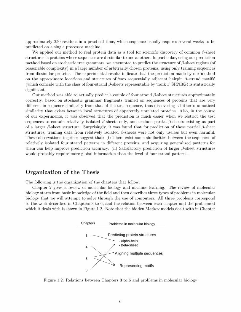
The following is the organization of the chapters that follow:Chapter 2 gives a review of molecular biology and machine learning. The review of molecular

biology starts from basic knowledge of the field and then describes three types of problems in molecularbiology that we will attempt to solve through the use of computers. All three problems correspondto the work described in Chapters 3 to 6, and the relation between each chapter and the problem(s)which it deals with is shown in Figure 1.2. Note that the hidden Markov models dealt with in Chapter

Chapters

3

4

5

6

Problems in molecular biology

Predicting protein structures

- Alpha-helix- Beta-sheet

Aligning multiple sequences

Representing motifs

Figure 1.2: Relations between Chapters 3 to 6 and problems in molecular biology

6

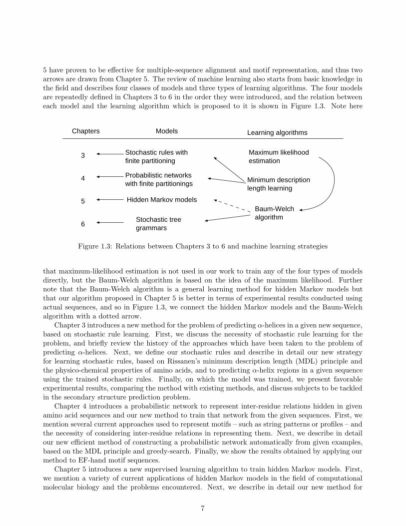
5 have proven to be effective for multiple-sequence alignment and motif representation, and thus twoarrows are drawn from Chapter 5. The review of machine learning also starts from basic knowledge inthe field and describes four classes of models and three types of learning algorithms. The four modelsare repeatedly defined in Chapters 3 to 6 in the order they were introduced, and the relation betweeneach model and the learning algorithm which is proposed to it is shown in Figure 1.3. Note here

Chapters

3

4

5

6

Models Learning algorithms

Stochastic rules withfinite partitioning

Probabilistic networkswith finite partitionings

Hidden Markov models

Stochastic treegrammars

Maximum likelihoodestimation

Minimum descriptionlength learning

Baum-Welchalgorithm

Figure 1.3: Relations between Chapters 3 to 6 and machine learning strategies

that maximum-likelihood estimation is not used in our work to train any of the four types of modelsdirectly, but the Baum-Welch algorithm is based on the idea of the maximum likelihood. Furthernote that the Baum-Welch algorithm is a general learning method for hidden Markov models butthat our algorithm proposed in Chapter 5 is better in terms of experimental results conducted usingactual sequences, and so in Figure 1.3, we connect the hidden Markov models and the Baum-Welchalgorithm with a dotted arrow.

Chapter 3 introduces a new method for the problem of predicting α-helices in a given new sequence,based on stochastic rule learning. First, we discuss the necessity of stochastic rule learning for theproblem, and briefly review the history of the approaches which have been taken to the problem ofpredicting α-helices. Next, we define our stochastic rules and describe in detail our new strategyfor learning stochastic rules, based on Rissanen’s minimum description length (MDL) principle andthe physico-chemical properties of amino acids, and to predicting α-helix regions in a given sequenceusing the trained stochastic rules. Finally, on which the model was trained, we present favorableexperimental results, comparing the method with existing methods, and discuss subjects to be tackledin the secondary structure prediction problem.

Chapter 4 introduces a probabilistic network to represent inter-residue relations hidden in givenamino acid sequences and our new method to train that network from the given sequences. First, wemention several current approaches used to represent motifs – such as string patterns or profiles – andthe necessity of considering inter-residue relations in representing them. Next, we describe in detailour new efficient method of constructing a probabilistic network automatically from given examples,based on the MDL principle and greedy-search. Finally, we show the results obtained by applying ourmethod to EF-hand motif sequences.

Chapter 5 introduces a new supervised learning algorithm to train hidden Markov models. First,we mention a variety of current applications of hidden Markov models in the field of computationalmolecular biology and the problems encountered. Next, we describe in detail our new method for

7

learning a hidden Markov model, training the system from not only examples which belong to theclass to be represented by the model, but also examples which do not. Finally, we present favorable ex-perimental results, comparing with two other existing methods, including the Baum-Welch algorithm,which is currently the most popular algorithm to train hidden Markov models.

Chapter 6 introduces a novel strategy for learning stochastic tree grammars to capture the long-range interactions which give rise to β-sheets, and to predict both the locations and structures ofβ-sheets in a given new sequence. In this chapter, we define stochastic tree grammars and describeour newly devised method for training them from given examples and using them to predict β-sheetsin a given new sequence with the trained grammars. Finally, we show experimental results obtainedby applying our method to a protein database, and describe possible future work to improve ourpredictive performance.

Chapter 7 gives concluding remarks of this thesis, and discusses the models and learning algorithmswhich should be considered in improving the accuracy of our current models and learning methods.

8

Chapter 2

Problems in Molecular Biology andMachine Learning

2.1 Computational Problems in Molecular Biology

In this section, we first present basic knowledge in molecular biology and next describe three compu-tational problems in the field – protein structure prediction, multiple sequence alignment and motifdetection – which comprise the subjects of this thesis, as well as being the principal themes of currentcomputational molecular biology.

The first problem, which is that of predicting protein structures for a given amino acid sequencethrough the use of computers, is the most crucial and difficult problem in the field and is the centraltheme of this thesis. The problem of predicting secondary structures, in particular, has been understudy since the 1970s, but satisfactory results have not yet been reached. The methods of predictingα-helices and β-sheets, which are the major two secondary structure classes, are discussed in Chapters3 and 6, respectively.

The second problem is that of aligning multiple sequences and using the result of the alignment,and of building a sequence ‘profile’ which corresponds to a representation form for all the alignedsequences. Sequence alignment is a very basic problem, and has been a goal in computational biologysince the early 1970s. Aligning multiple sequences belonging to a class has already been achieved ona practical level, at which the profile for the class, which is obtained by the alignment, is used asa tool for database search. In recent few years, however, a statistical representation newly appliedin this field – ‘hidden Markov model’ – has been proposed for use both in aligning sequences and incalculating profiles of the sequences at the same time. Chapter 5 is concerned with this problem, anddescribing a new learning algorithm for hidden Markov models.

The third problem is related to ‘motifs’, which typically indicate common patterns of biologicalsequences belonging to a certain class. The main research theme in this problem is the best methodto use to represent a motif in order to detect the motif with high accuracy in given sequences. Motifswhich had been simply represented by string patterns so far, are also being replaced by new statisticalrepresentations such as hidden Markov models. Chapters 4 and 5 deal with this problem and Chapter4 proposes a new method for representing motifs, instead of simple string patterns.

The above three problems are not the only problems in molecular biology. In addition, well-known major computational problems include finding genes in nucleotide sequences, phylogenetic treereconstruction, predicting the structure of nucleotide sequences, etc. These problems remain unsolved,despite being well-researched in the computational molecular biology field.

9

2.1.1 Fundamentals of Molecular Biology

Basic Terms

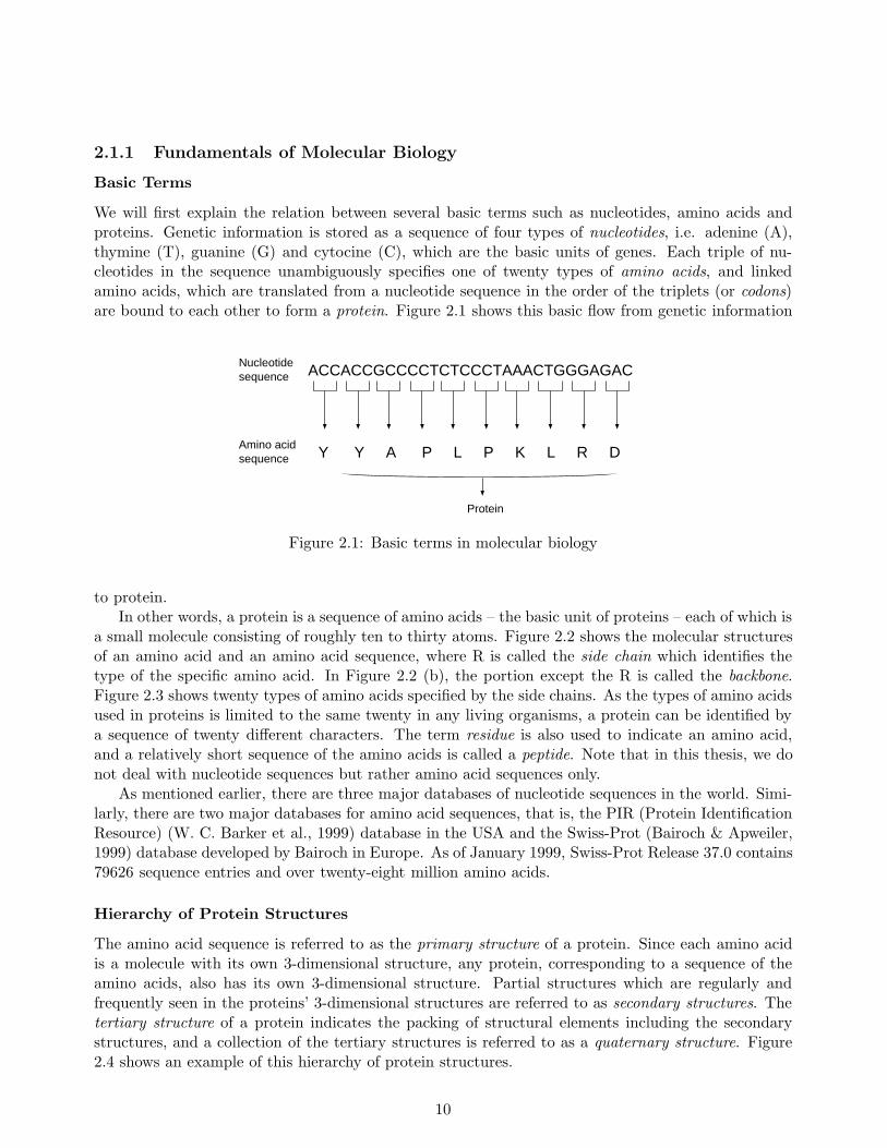
We will first explain the relation between several basic terms such as nucleotides, amino acids andproteins. Genetic information is stored as a sequence of four types of nucleotides, i.e. adenine (A),thymine (T), guanine (G) and cytocine (C), which are the basic units of genes. Each triple of nu-cleotides in the sequence unambiguously specifies one of twenty types of amino acids, and linkedamino acids, which are translated from a nucleotide sequence in the order of the triplets (or codons)are bound to each other to form a protein. Figure 2.1 shows this basic flow from genetic information

Nucleotidesequence

Amino acidsequence

ACCACCGCCCCTCTCCCTAAACTGGGAGAC

Y Y A P L P K L R D

Protein

Figure 2.1: Basic terms in molecular biology

to protein.In other words, a protein is a sequence of amino acids – the basic unit of proteins – each of which is

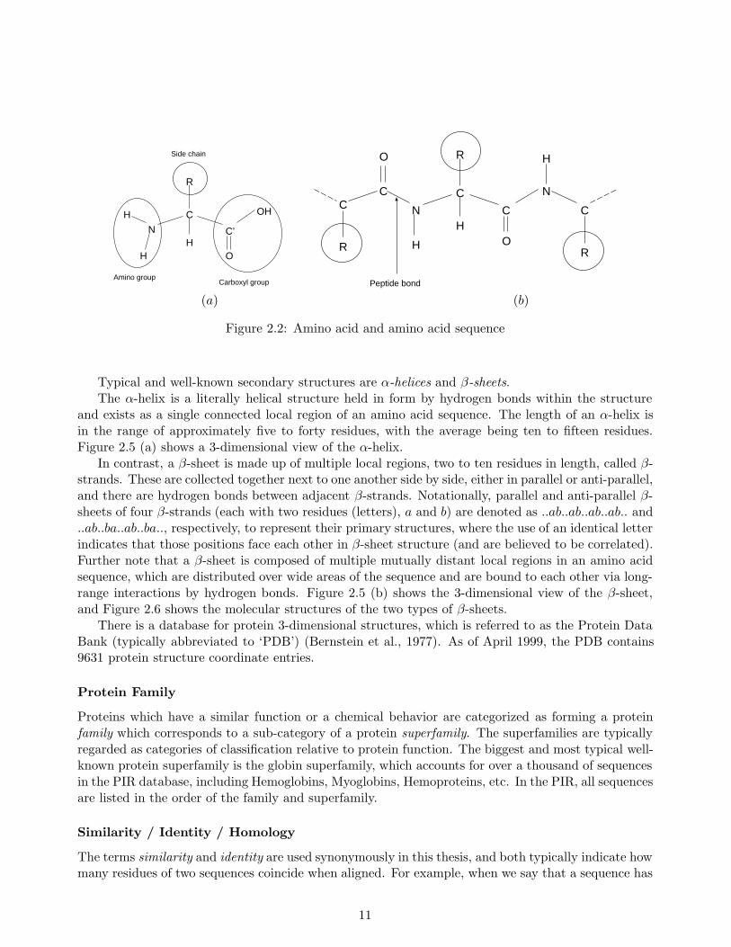
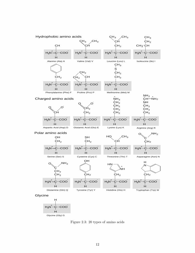
a small molecule consisting of roughly ten to thirty atoms. Figure 2.2 shows the molecular structuresof an amino acid and an amino acid sequence, where R is called the side chain which identifies thetype of the specific amino acid. In Figure 2.2 (b), the portion except the R is called the backbone.Figure 2.3 shows twenty types of amino acids specified by the side chains. As the types of amino acidsused in proteins is limited to the same twenty in any living organisms, a protein can be identified bya sequence of twenty different characters. The term residue is also used to indicate an amino acid,and a relatively short sequence of the amino acids is called a peptide. Note that in this thesis, we donot deal with nucleotide sequences but rather amino acid sequences only.

As mentioned earlier, there are three major databases of nucleotide sequences in the world. Simi-larly, there are two major databases for amino acid sequences, that is, the PIR (Protein IdentificationResource) (W. C. Barker et al., 1999) database in the USA and the Swiss-Prot (Bairoch & Apweiler,1999) database developed by Bairoch in Europe. As of January 1999, Swiss-Prot Release 37.0 contains79626 sequence entries and over twenty-eight million amino acids.

Hierarchy of Protein Structures

The amino acid sequence is referred to as the primary structure of a protein. Since each amino acidis a molecule with its own 3-dimensional structure, any protein, corresponding to a sequence of theamino acids, also has its own 3-dimensional structure. Partial structures which are regularly andfrequently seen in the proteins’ 3-dimensional structures are referred to as secondary structures. Thetertiary structure of a protein indicates the packing of structural elements including the secondarystructures, and a collection of the tertiary structures is referred to as a quaternary structure. Figure2.4 shows an example of this hierarchy of protein structures.

10

C

R

N

H

H

C’

OH

OH

Side chain

Amino groupCarboxyl group

C

R

N

C

H

C

OH

O

C

R

C

N

H

R

Peptide bond

(a) (b)

Figure 2.2: Amino acid and amino acid sequence

Typical and well-known secondary structures are α-helices and β-sheets.The α-helix is a literally helical structure held in form by hydrogen bonds within the structure

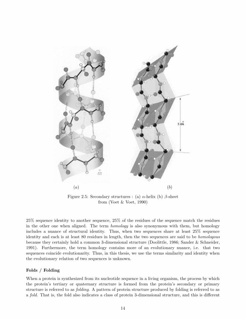
and exists as a single connected local region of an amino acid sequence. The length of an α-helix isin the range of approximately five to forty residues, with the average being ten to fifteen residues.Figure 2.5 (a) shows a 3-dimensional view of the α-helix.

In contrast, a β-sheet is made up of multiple local regions, two to ten residues in length, called β-strands. These are collected together next to one another side by side, either in parallel or anti-parallel,and there are hydrogen bonds between adjacent β-strands. Notationally, parallel and anti-parallel β-sheets of four β-strands (each with two residues (letters), a and b) are denoted as ..ab..ab..ab..ab.. and..ab..ba..ab..ba.., respectively, to represent their primary structures, where the use of an identical letterindicates that those positions face each other in β-sheet structure (and are believed to be correlated).Further note that a β-sheet is composed of multiple mutually distant local regions in an amino acidsequence, which are distributed over wide areas of the sequence and are bound to each other via long-range interactions by hydrogen bonds. Figure 2.5 (b) shows the 3-dimensional view of the β-sheet,and Figure 2.6 shows the molecular structures of the two types of β-sheets.

There is a database for protein 3-dimensional structures, which is referred to as the Protein DataBank (typically abbreviated to ‘PDB’) (Bernstein et al., 1977). As of April 1999, the PDB contains9631 protein structure coordinate entries.

Protein Family

Proteins which have a similar function or a chemical behavior are categorized as forming a proteinfamily which corresponds to a sub-category of a protein superfamily. The superfamilies are typicallyregarded as categories of classification relative to protein function. The biggest and most typical well-known protein superfamily is the globin superfamily, which accounts for over a thousand of sequencesin the PIR database, including Hemoglobins, Myoglobins, Hemoproteins, etc. In the PIR, all sequencesare listed in the order of the family and superfamily.

Similarity / Identity / Homology

The terms similarity and identity are used synonymously in this thesis, and both typically indicate howmany residues of two sequences coincide when aligned. For example, when we say that a sequence has

11

Hydrophobic amino acidsCH

C

CH

H N COO

HAlanine (Ala) A

CH

Valine (Val) V

CH

Leucine (Leu) L

CH

Isoleucine (Ile) I

CH CH

CH

CH

CH

CH

CH

3

3 3

3 3

2

2

3

3

CHCH

Phenylalanine (Phe) F

CH

Proline (Pro) P

2

CH

Methionine (Met) M

CH CH

2

S

CH3

22

2

Charged amino acids

+ -CH N COO

H

3+ -

CH N COO

H

3+ -

CH N COO

H

3+ -

CH N COO

H

3+ -

CH N COO

H

+ -CH N COO

H

3+ -

2

O

C

CH

H N COO

HAspartic Acid (Asp) D

CH

Glutamic Acid (Glu) E

CH

Lysine (Lys) K Arginine (Arg) R

O

CHCHCH

3

3

2

2

+ -CH N COO

H

3+ -

CH N COO

H

3+ -

CH N COO

H

3+ -

OO

CH

-

-

2

NH

2

2

CHCHCHNH

2

2

CH

22

NHNH

+ +2

2

Polar amino acids

C

CH

H N COO

HSerine (Ser) S

CH

Cysteine (Cys) C Threonine (Thr) T

CH

Asparagine (Asn) N

CH

HO CH

3

3

+ -CH N COO

H

3+ -

CH N COO

H

3+ -

CH N COO

H

3+ -

C

CH

H N COO

HGlutamine (Gln) Q

CH

Tyrosine (Tyr) Y

CH

Histidine (His) H

CH

Tryptophan (Trp) W

HN

NH

3

2

2

+ -CH N COO

H

3+ -

CH N COO

H

3+ -

CH N COO

H

3+ -

H

Glycine (Gly) G

OH SH

C

O NH

CHC

O NH

OH HN

222

2

2

2

2 2

+

Glycine

CH N COO

H

3+ -

Figure 2.3: 20 types of amino acids

12

Figure 2.4: Hierarchy of protein structures

from http://www.eng.rpi.edu/dept/chem-eng/Biotech-Environ/PRECIP/precpintro.html

13

(a) (b)

Figure 2.5: Secondary structures : (a) α-helix (b) β-sheetfrom (Voet & Voet, 1990)

25% sequence identity to another sequence, 25% of the residues of the sequence match the residuesin the other one when aligned. The term homology is also synonymous with them, but homologyincludes a nuance of structural identity. Thus, when two sequences share at least 25% sequenceidentity and each is at least 80 residues in length, then the two sequences are said to be homologousbecause they certainly hold a common 3-dimensional structure (Doolittle, 1986; Sander & Schneider,1991). Furthermore, the term homology contains more of an evolutionary nuance, i.e. that twosequences coincide evolutionarity. Thus, in this thesis, we use the terms similarity and identity whenthe evolutionary relation of two sequences is unknown.

Folds / Folding

When a protein is synthesized from its nucleotide sequence in a living organism, the process by whichthe protein’s tertiary or quaternary structure is formed from the protein’s secondary or primarystructure is referred to as folding. A pattern of protein structure produced by folding is referred to asa fold. That is, the fold also indicates a class of protein 3-dimensional structure, and this is different

14

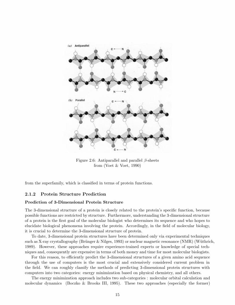
Figure 2.6: Antiparallel and parallel β-sheetsfrom (Voet & Voet, 1990)

from the superfamily, which is classified in terms of protein functions.

2.1.2 Protein Structure Prediction

Prediction of 3-Dimensional Protein Structure

The 3-dimensional structure of a protein is closely related to the protein’s specific function, becausepossible functions are restricted by structure. Furthermore, understanding the 3-dimensional structureof a protein is the first goal of the molecular biologist who determines its sequence and who hopes toelucidate biological phenomena involving the protein. Accordingly, in the field of molecular biology,it is crucial to determine the 3-dimensional structure of protein.

To date, 3-dimensional protein structures have been determined only via experimental techniquessuch as X-ray crystallography (Brunger & Nilges, 1993) or nuclear magnetic resonance (NMR) (Wuthrich,1989). However, these approaches require experience-trained experts or knowledge of special tech-niques and, consequently are expensive in terms of both money and time for most molecular biologists.

For this reason, to efficiently predict the 3-dimensional structures of a given amino acid sequencethrough the use of computers is the most crucial and extensively considered current problem inthe field. We can roughly classify the methods of predicting 3-dimensional protein structures withcomputers into two categories: energy minimization based on physical chemistry, and all others.

The energy minimization approach includes two sub-categories : molecular orbital calculation andmolecular dynamics (Boczko & Brooks III, 1995). These two approaches (especially the former)

15

Predict protein 3D structures

Energy minimization

Molecular orbitalcalculation

Molecular dynamics

OthersHomology modeling

Inverse folding

{{

{ Secondary structureprediction, etc.

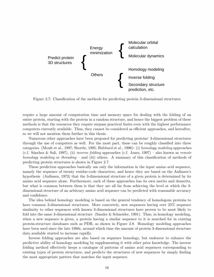
Figure 2.7: Classification of the methods for predicting protein 3-dimensional structures

require a large amount of computation time and memory space for dealing with the folding of anentire protein, starting with the protein in a random structure, and hence the biggest problem of thesemethods is that the resources they require surpass practical limits even with the highest performancecomputers currently available. Thus, they cannot be considered as efficient approaches, and hereafter,so we will not mention them further in this thesis.

Numerous other approaches have been proposed for predicting proteins’ 3-dimensional structuresthrough the use of computers as well. For the most part, these can be roughly classified into threecategories (Moult et al., 1997; Shortle, 1995; Hubbard et al., 1996): (i) homology modeling approaches(c.f. Sanchez & Sali, 1997), (ii) inverse folding approaches (c.f. Jones, 1997) – also known as remotehomology modeling or threading – and (iii) others. A summary of this classification of methods ofpredicting protein structures is shown in Figure 2.7.

These prediction approaches basically use only the information in the input amino acid sequence,namely the sequence of twenty residue-code characters, and hence they are based on the Anfinsen’shypothesis (Anfinsen, 1973) that the 3-dimensional structure of a given protein is determined by itsamino acid sequence alone. Furthermore, each of these approaches has its own merits and demerits,but what is common between them is that they are all far from achieving the level at which the 3-dimensional structure of an arbitrary amino acid sequence can be predicted with reasonable accuracyand confidence.

The idea behind homology modeling is based on the general tendency of homologous proteins tohave common 3-dimensional structures. More concretely, new sequences having over 25% sequencesimilarity to other sequences with known 3-dimensional structures have proven to be most likely tofold into the same 3-dimensional structure (Sander & Schneider, 1991). Thus, in homology modeling,when a new sequence is given, a protein having a similar sequence to it is searched for in existingprotein-structure databases such as PDB, as shown in Figure 2.8. Homology modeling approacheshave been used since the late 1980s, around which time the amount of protein 3-dimensional structuredata available started to increase rapidly.

Inverse folding approaches are also based on sequence homology, but endeavor to enhance thepredictive ability of homology modeling by supplementing it with other prior knowledge. The inversefolding method effectively keeps a catalogue of patterns of amino acid sequences corresponding toexisting types of protein structures, and predicts the structures of new sequences by simply findingthe most appropriate pattern that matches the input sequence.

16

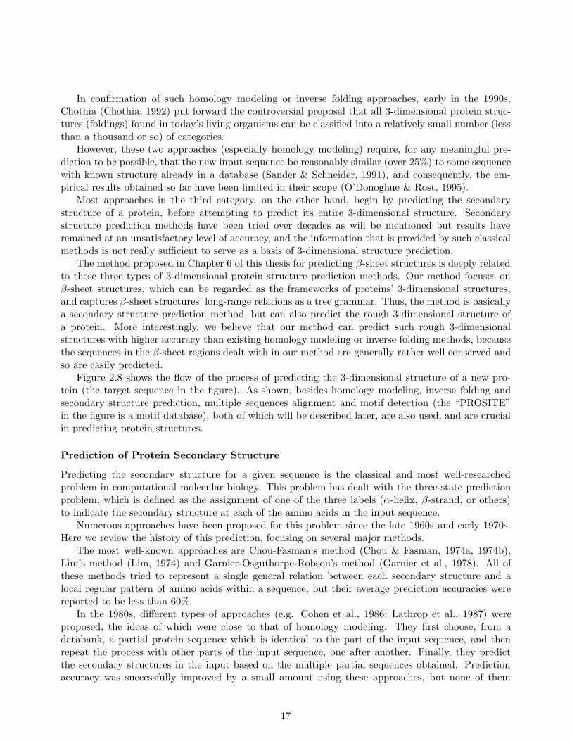
In confirmation of such homology modeling or inverse folding approaches, early in the 1990s,Chothia (Chothia, 1992) put forward the controversial proposal that all 3-dimensional protein struc-tures (foldings) found in today’s living organisms can be classified into a relatively small number (lessthan a thousand or so) of categories.

However, these two approaches (especially homology modeling) require, for any meaningful pre-diction to be possible, that the new input sequence be reasonably similar (over 25%) to some sequencewith known structure already in a database (Sander & Schneider, 1991), and consequently, the em-pirical results obtained so far have been limited in their scope (O’Donoghue & Rost, 1995).

Most approaches in the third category, on the other hand, begin by predicting the secondarystructure of a protein, before attempting to predict its entire 3-dimensional structure. Secondarystructure prediction methods have been tried over decades as will be mentioned but results haveremained at an unsatisfactory level of accuracy, and the information that is provided by such classicalmethods is not really sufficient to serve as a basis of 3-dimensional structure prediction.

The method proposed in Chapter 6 of this thesis for predicting β-sheet structures is deeply relatedto these three types of 3-dimensional protein structure prediction methods. Our method focuses onβ-sheet structures, which can be regarded as the frameworks of proteins’ 3-dimensional structures,and captures β-sheet structures’ long-range relations as a tree grammar. Thus, the method is basicallya secondary structure prediction method, but can also predict the rough 3-dimensional structure ofa protein. More interestingly, we believe that our method can predict such rough 3-dimensionalstructures with higher accuracy than existing homology modeling or inverse folding methods, becausethe sequences in the β-sheet regions dealt with in our method are generally rather well conserved andso are easily predicted.

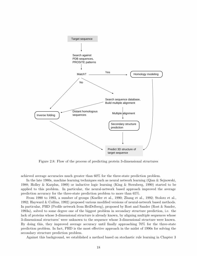
Figure 2.8 shows the flow of the process of predicting the 3-dimensional structure of a new pro-tein (the target sequence in the figure). As shown, besides homology modeling, inverse folding andsecondary structure prediction, multiple sequences alignment and motif detection (the “PROSITE”in the figure is a motif database), both of which will be described later, are also used, and are crucialin predicting protein structures.

Prediction of Protein Secondary Structure

Predicting the secondary structure for a given sequence is the classical and most well-researchedproblem in computational molecular biology. This problem has dealt with the three-state predictionproblem, which is defined as the assignment of one of the three labels (α-helix, β-strand, or others)to indicate the secondary structure at each of the amino acids in the input sequence.

Numerous approaches have been proposed for this problem since the late 1960s and early 1970s.Here we review the history of this prediction, focusing on several major methods.

The most well-known approaches are Chou-Fasman’s method (Chou & Fasman, 1974a, 1974b),Lim’s method (Lim, 1974) and Garnier-Osguthorpe-Robson’s method (Garnier et al., 1978). All ofthese methods tried to represent a single general relation between each secondary structure and alocal regular pattern of amino acids within a sequence, but their average prediction accuracies werereported to be less than 60%.

In the 1980s, different types of approaches (e.g. Cohen et al., 1986; Lathrop et al., 1987) wereproposed, the ideas of which were close to that of homology modeling. They first choose, from adatabank, a partial protein sequence which is identical to the part of the input sequence, and thenrepeat the process with other parts of the input sequence, one after another. Finally, they predictthe secondary structures in the input based on the multiple partial sequences obtained. Predictionaccuracy was successfully improved by a small amount using these approaches, but none of them

17

Target sequence

Search againstPDB sequences,PROSITE patterns

Homology modeling

Distant homologoussequencesInverse folding

Match?

Predict 3D structure of target sequence

Search sequence database,Build multiple alignment

Multiple alignment

Secondary structureprediction

Yes

No

Figure 2.8: Flow of the process of predicting protein 3-dimensional structures

achieved average accuracies much greater than 60% for the three-state prediction problem.In the late 1980s, machine learning techniques such as neural network learning (Qian & Sejnowski,

1988; Holley & Karplus, 1989) or inductive logic learning (King & Sternberg, 1990) started to beapplied to this problem. In particular, the neural-network based approach improved the averageprediction accuracy for the three-state prediction problem to more than 65%.

From 1990 to 1993, a number of groups (Kneller et al., 1990; Zhang et al., 1992; Stolorz et al.,1992; Hayward & Collins, 1992) proposed various modified versions of neural-network based methods.In particular, PHD (Profile network from HeiDelberg), proposed by Rost and Sander (Rost & Sander,1993a), solved to some degree one of the biggest problem in secondary structure prediction, i.e. thelack of proteins whose 3-dimensional structure is already known, by aligning multiple sequences whose3-dimensional structures’ were unknown to the sequence whose 3-dimensional structure were known.By doing this, they improved average accuracy until finally approaching 70% for the three-stateprediction problem. In fact, PHD is the most effective approach in the midst of 1990s for solving thesecondary structure prediction problem.

Against this background, we established a method based on stochastic rule learning in Chapter 3

18

of this thesis, focusing on predicting α-helices only, and achieves a prediction accuracy exceeding 80%(almost the same level as that of the PHD in predicting α-helices only). Moreover, our method hasthe advantage of being able to provide understandable rules for predicting α-helices in a given newsequence, while the PHD cannot.

A major criticism of secondary structure prediction is that the information provided by themis essentially 1-dimensional in nature (O’Donoghue & Rost, 1995) and thus is not ideal as a basisof 3-dimensional structure prediction, even if it provides high prediction accuracy. This criticism isespecially true of β-sheet prediction, since as mentioned earlier, β-sheets consist of several separatedportions of a sequence while existing secondary structure prediction methods, including PHD, providethe information only as a 1-dimensional label sequence, in which a label (α-helix, β-sheet or others) isassigned to each of the amino acids in the input sequence, and do not consider the relations betweenmutually distant portions in the sequence, such as which β-strands belong to the same β-sheet, etc.

In response to this criticism, we established a novel method in Chapter 6, which learns not onlylocal properties as a 1-dimensional sequence, but also the long-range relations of β-sheets. In thissense, our method is the first to break past the existing secondary structure framework in which 1-dimensional prediction is done, to extend it into a proper preliminary tool for the prediction of theglobal 3-dimensional structures of proteins.

2.1.3 Multiple Sequence Alignment - Profile Calculation

As shown in Figure 2.8, in the homology modeling approach to prediction of protein structure, we needto search for sequences having similarity to the input sequence. To measure the similarity betweentwo sequences, techniques for aligning sequences with reasonable accuracy and speed are required.

Any molecular biologist who determines a nucleotide sequence first tries to find similar sequencesin the major databases, in which sequences whose structures and/or functions are already known areavailable for search. If one is fortunate enough to find a large number of similar sequences, one canstart the next step of inferring the function or structure of the new sequence using them (Altschulet al., 1994).

It should be clear from the above that it is a crucial problem in molecular biology to align sequencesaccurately and rapidly. One major problem in aligning two given sequences (referred to as pairwisealignment) is that blanks (referred to as gaps) made up of sub-sequences to be ignored are allowed tobe inserted in each of the two sequences. A method based on the dynamic programming (hereafterreferred to as the DP) has been used to align sequences including gaps.

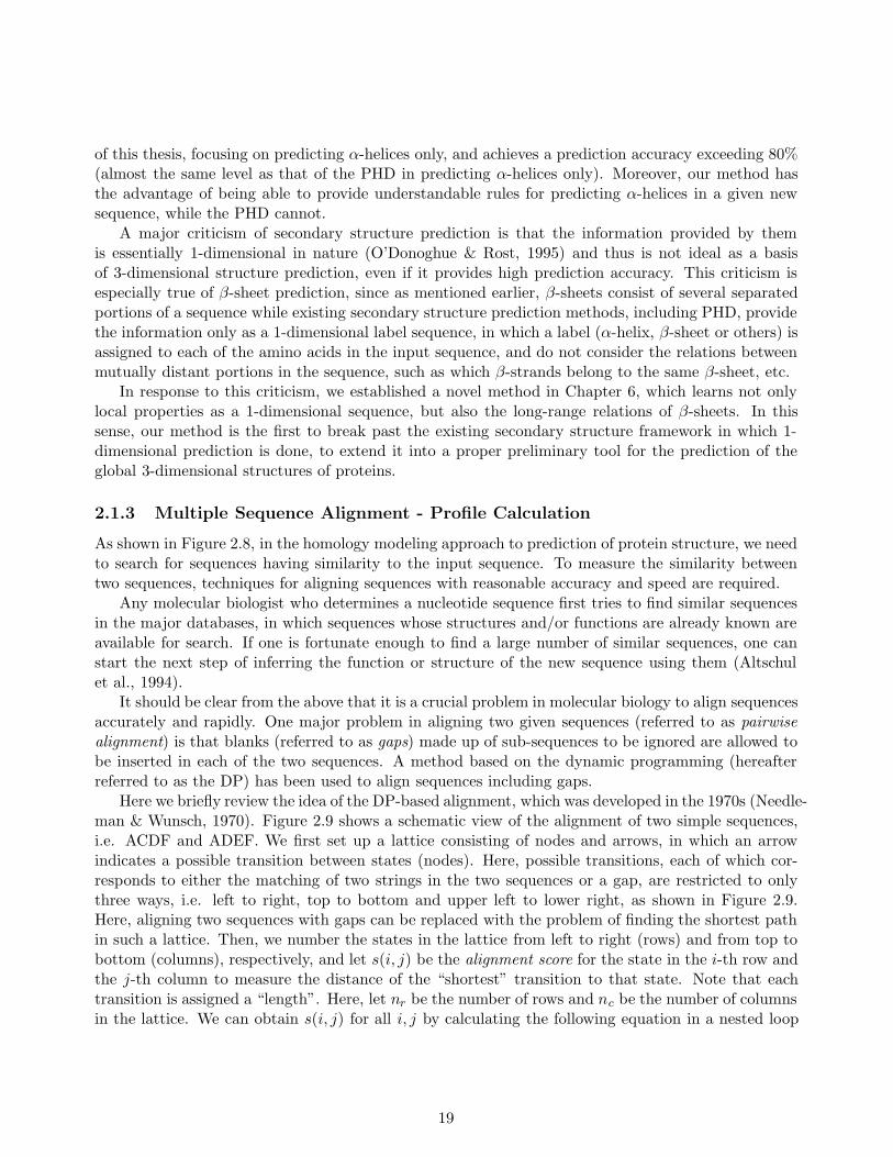
Here we briefly review the idea of the DP-based alignment, which was developed in the 1970s (Needle-man & Wunsch, 1970). Figure 2.9 shows a schematic view of the alignment of two simple sequences,i.e. ACDF and ADEF. We first set up a lattice consisting of nodes and arrows, in which an arrowindicates a possible transition between states (nodes). Here, possible transitions, each of which cor-responds to either the matching of two strings in the two sequences or a gap, are restricted to onlythree ways, i.e. left to right, top to bottom and upper left to lower right, as shown in Figure 2.9.Here, aligning two sequences with gaps can be replaced with the problem of finding the shortest pathin such a lattice. Then, we number the states in the lattice from left to right (rows) and from top tobottom (columns), respectively, and let s(i, j) be the alignment score for the state in the i-th row andthe j-th column to measure the distance of the “shortest” transition to that state. Note that eachtransition is assigned a “length”. Here, let nr be the number of rows and nc be the number of columnsin the lattice. We can obtain s(i, j) for all i, j by calculating the following equation in a nested loop

19

A

C

D

F

A D E F

ACDF

ADEF

ACD . F

A . DEF

Figure 2.9: Aligning two sequences based on dynamic programming

with increasing values of i and j (i = 1, · · · , nr, j = 1, · · · , nc).

s(i, j) = min

s(i − 1, j) +Cas(i, j − 1) +Cas(i − 1, j − 1) +Cb,

where Ca is a kind of gap penalty, Cb is the score corresponding to a direct match between a pair ofa certain kind of amino acids, and Ca > Cb > 0. Each s(i, j) which is used in calculating the finals(i, j) at which i = nr and j = nc, is then regarded as a state in the shortest path.

The values Ca and Cb can be varied depending on the types of the two amino acids, using atransition matrix such as the one determined by Dayhoff (Dayhoff et al., 1978). In the examplesshown in Figure 2.9, the sequences are aligned as ACD.F and A.DEF. This DP-based alignment fortwo sequences can be expanded into one for aligning multiple sequences in several ways, such asiteration (Barton & Sternberg, 1987; Taylor, 1987; Berger & Munson, 1991) or the use of parallelcomputers (Ishikawa et al., 1993), but such multiple-sequence alignment has not yet been solvedcompletely and is an active research area studied at the present time.

A profile is a matrix representing the proportional distribution of amino acids at each positionwhen multiple sequences are aligned (Taylor, 1986b; Gribskov et al., 1987). For example, if we alignthree simple sequences, ACEF, ADEF and AGEF, the amino acids at the second position in thealigned sequences will be evenly split between C, D and G while other positions will be fixed to onlyone type of amino acid, so the profile for this simple example is as follows:

1 2 3 4A 1.0 0.0 0.0 0.0C 0.0 0.333 0.0 0.0D 0.0 0.333 0.0 0.0E 0.0 0.0 1.0 0.0F 0.0 0.0 0.0 1.0G 0.0 0.333 0.0 0.0

A profile calculated for multiple sequences belonging to a single category, such as a family or asuperfamily, is expected to represent a typical sequence or a representative model of the category.

20

Thus, if we have calculated the profiles for all categories of sequences, when given a new sequence,we can easily find the closest-matching category by comparing the sequence with each calculatedprofile or with parts of profiles. For that reason, in place of such simple amino acid distributions asthat shown above, methods of representing profiles with reasonably high accuracy for specific purposessuch as sequence classification have recently been one of the hottest areas of research in computationalmolecular biology.

In particular, in 1993 to 1994, hidden Markov models have been proposed, both for multiple-sequence alignment and calculating profiles at the same time (Krogh et al., 1994a; Baldi et al., 1994).The hidden Markov model is a powerful statistical model which allows us to handle sequences includingrepetition and gaps, and is at present the most influential method in multiple sequence alignment andrelated areas (Taubes, 1996). For example, even in the inverse folding approach to predicting proteins’3-dimensional structures, hidden Markov models have been used as basic catalogue entries for modelingeach protein structure class (Moult et al., 1997; Shortle, 1995). Details of the hidden Markov modelwill be described in Sections 2.2.2 and 2.2.3, and we will propose a new learning method for applyinghidden Markov models to sequence discrimination in Chapter 5.

2.1.4 Motif Detection / Discrimination / Classification

The term motif is used in two different meanings, as occasion demands.The first definition, which is the most general one, is as a common short sub-string pattern seen in

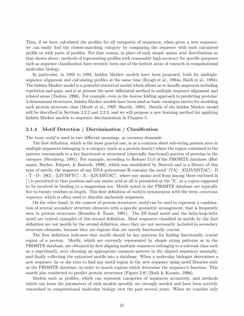
multiple sequences belonging to a category (such as a protein family) where the region contained in thepattern corresponds to a key functional or structural (especially functional) portion of proteins in thecategory (Sternberg, 1991). For example, according to Release 15.0 of the PROSITE database (Hof-mann, Bucher, Falquet, & Bairoch, 1999), which was established by Bairoch and is a library of thistype of motifs, the sequence of any DNA polymerase B contains the motif ‘[YA] - [GLIVMSTAC] - D- T - D - [SG] - [LIVMFTC] - X - [LIVMSTAC]’, where any amino acid from among those enclosed in[ ] is permitted at that position and any amino acid at all is permitted at the ‘X’, at a region supposedto be involved in binding to a magnesium ion. Motifs noted in the PROSITE database are typicallyfive to twenty residues in length. This first definition of motif is synonymous with the term consensussequence, which is often used to describe nucleotide sequences.

On the other hand, in the context of protein structures, motif can be used to represent a combina-tion of several secondary structure elements with a specific geometric arrangement, that is frequentlyseen in protein structures (Branden & Tooze, 1991). The EF-hand motif and the helix-loop-helixmotif are typical examples of this second definition. Most sequences classified as motifs by the firstdefinition are not motifs by the second definition, since they are not necessarily included in secondarystructure elements, because they are regions that are merely functionally crucial.

The first definition indicates that motifs should be key patterns for finding functionally crucialregion of a protein. Motifs, which are currently represented by simple string patterns as in thePROSITE database, are obtained by first aligning multiple sequences belonging to a relevant class suchas a superfamily, next choosing an appropriate common pattern in the aligned sequences manually,and finally collecting the extracted motifs into a database. When a molecular biologist determines anew sequence, he or she tries to find any motif region in the new sequence using motif libraries suchas the PROSITE database, in order to search regions which determine the sequence’s function. Thissearch also conducted to predict protein structures (Figure 2.8) (Bork & Koonin, 1996).

Models such as profiles, which can represent categories of sequences accurately, and methodswhich can learn the parameters of such models speedily are strongly needed and have been activelyresearched in computational molecular biology over the past several years. When we consider only

21

short sequences as targets, we can say that obtaining profiles and representing motifs lead to a commonproblem. To solve it, a number of stochastic or statistical models including hidden Markov models inplace of available simple motifs, have been proposed to date (Durbin et al., 1998). In this thesis, aswell, we define probabilistic networks with finite partitionings to represent motifs (Chapter 4) , andin addition, establish a new learning method for hidden Markov models (Chapter 5).

2.2 Machine Learning

In this section, we first explain the fundamental concepts and terms of the field of machine learning,then describe four types of learning-model classes, each of which is used in a corresponding subsequentchapter, and finally describe three types of algorithms, which are strongly concerned with learningthe four model classes (Figure 1.3).

Note that machine learning basically refers to all types of automatic knowledge acquisition throughthe use of computers. Learning from examples, the approach used in this thesis, is merely one wayof tackling the basic problems of machine learning, but it is the principal approach used in currentresearch.

2.2.1 Fundamentals of Machine Learning

As briefly mentioned in Chapter 1, the subject of machine learning is to provide machines with learningabilities, which has been also one of the major goals of artificial intelligence in the field of computerscience.

What is Learning?

Since in the early stages of the field of artificial intelligence, the philosophical question ‘What islearning ?’ has been repeated any number of times and the general answer has been that learning isany of various kinds of changes. We introduce some of them here.

Simon (Simon, 1983) characterized the change in detail:

Learning denotes changes in the system that are adaptive in the sense that theyenable the system to do the same task or tasks drawn from the same populationmore effectively the next time.

Minsky (Minsky, 1986) mentioned that it is merely any useful change:

Learning is making useful changes in our mind.

Michalski (Michalski, 1986) noted that the change has a representation:

Learning is constructing or modifying representations of what is being experienced.

As Michalski defined, we might grasp the meaning of learning as constructing or modifying rep-resentations from obtained examples. Here, let us consider a simple example of a learning problem,which classifies given examples into two classes, i.e. fruits and vegetables. In this problem, the learneris presented with a finite number of examples, each of which has two attributes, the color and weight,and a class. That is, the examples fit the form shown in the following table:

22

No. Color Weight(g) Class

1 Yellow 20 Fruit2 Green 28 Vegetable3 Red 24 Vegetable4 Orange 17 Fruit· · ·

From the examples, the learner may find a rule for classifying the examples into two categories. Forinstance, when given an example, if its color is yellow or orange and its weight is less than 22 grams,the example is a fruit. The classification rule (for short, rule) is nothing else but a representationobtained from the examples, as Michalski mentioned, and is a function that can be represented as amapping of a two-dimensional value (the attributes) as input and to a scalar value (the correspondingclass of the example) as output. Here, note that the rule is a deterministic rule in terms of prediction,i.e. that the class of any example is unambiguously determined by the rule.

Further note that in this example, each input has a label specifying its class, e.g. a fruit or avegetable; such learning (with labeled examples) is referred to as supervised learning. Conversely,learning with examples which have no labels, is referred to as unsupervised learning.

Stochastic Rules

Here, let us consider another example in which we would like to learn a classification rule for predictingwhether the weather will be good or not tomorrow based on all the data available until now. In thisexample, the weather is basically an uncertain event, and it would be impossible to forecast theweather with high accuracy using a deterministic rule. In such situations, it is generally desirableto use rules with assigned probabilities, called stochastic rules, to achieve high prediction accuracy.Also, in the cases which can include unexpected errors or noise, learning of a stochastic rule would bepreferable (more robust) than learning a deterministic one.

The term learning is often replaced by several other terms such as training, estimation and fitting.The term estimation is usually used in the field of statistical inference. This term has been usedanalogously in the machine learning field, because learning stochastic rules from given examples canbe regarded as estimating input-output correlations in statistical inference.

Models / Parameters

The term model is an extremely elusive term, but generally indicates a form of representation for therules or functions to be learned from examples. In general, a model includes parameters which are tobe learned from examples.

We note here that not only the learning of the parameters of a model, but also the selecting amodel itself can be an objective of learning. In other words, the number of parameters in a model canbe learned from examples. This type of learning is referred to as model estimation or model selection,while learning only the values of the parameters of a model is referred to as parameter estimation ormodel fitting.

2.2.2 Model Classes

In this section, we define four classes of models, which are then described in detail in Chapters 3to 6, in the order presented. They are all stochastic models that learn stochastic rules from givenexamples. Note that there are numerous other models in use in the machine learning field, including,for example, artificial neural networks.

23

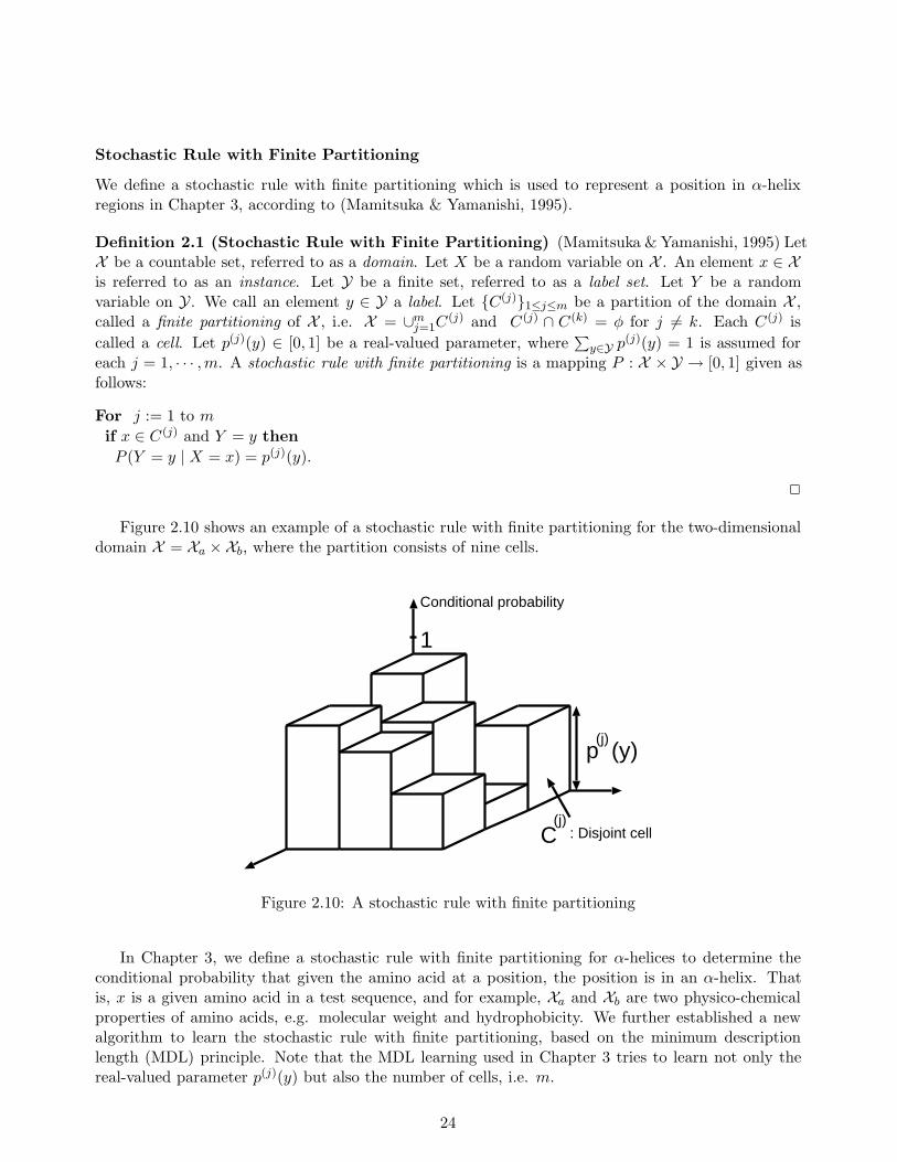
Stochastic Rule with Finite Partitioning

We define a stochastic rule with finite partitioning which is used to represent a position in α-helixregions in Chapter 3, according to (Mamitsuka & Yamanishi, 1995).

Definition 2.1 (Stochastic Rule with Finite Partitioning) (Mamitsuka & Yamanishi, 1995) LetX be a countable set, referred to as a domain. Let X be a random variable on X . An element x ∈ Xis referred to as an instance. Let Y be a finite set, referred to as a label set. Let Y be a randomvariable on Y. We call an element y ∈ Y a label. Let {C(j)}1≤j≤m be a partition of the domain X ,called a finite partitioning of X , i.e. X = ∪m

j=1C(j) and C(j) ∩ C(k) = φ for j 6= k. Each C(j) is

called a cell. Let p(j)(y) ∈ [0, 1] be a real-valued parameter, where∑

y∈Y p(j)(y) = 1 is assumed foreach j = 1, · · · ,m. A stochastic rule with finite partitioning is a mapping P : X × Y → [0, 1] given asfollows:

For j := 1 to m

if x ∈ C(j) and Y = y then

P (Y = y | X = x) = p(j)(y).

2

Figure 2.10 shows an example of a stochastic rule with finite partitioning for the two-dimensionaldomain X = Xa ×Xb, where the partition consists of nine cells.

p (y)(j)

1

C (j)

: Disjoint cell

Conditional probability

Figure 2.10: A stochastic rule with finite partitioning

In Chapter 3, we define a stochastic rule with finite partitioning for α-helices to determine theconditional probability that given the amino acid at a position, the position is in an α-helix. Thatis, x is a given amino acid in a test sequence, and for example, Xa and Xb are two physico-chemicalproperties of amino acids, e.g. molecular weight and hydrophobicity. We further established a newalgorithm to learn the stochastic rule with finite partitioning, based on the minimum descriptionlength (MDL) principle. Note that the MDL learning used in Chapter 3 tries to learn not only thereal-valued parameter p(j)(y) but also the number of cells, i.e. m.

24

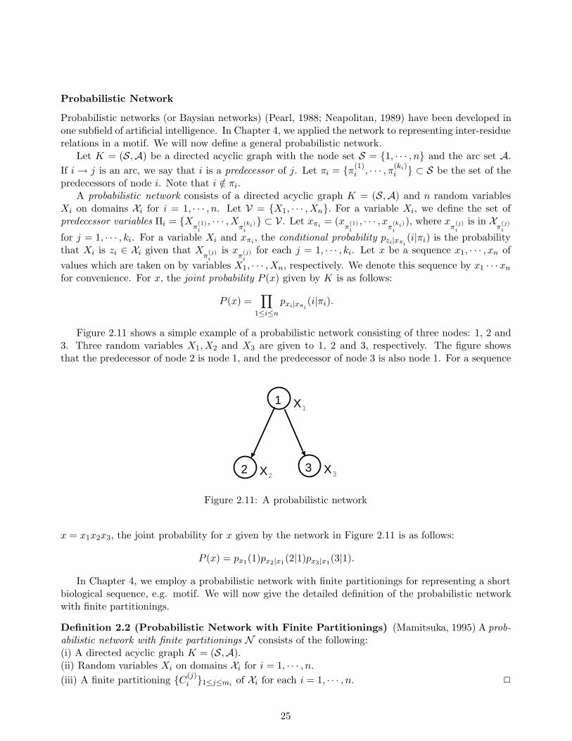
Probabilistic Network

Probabilistic networks (or Baysian networks) (Pearl, 1988; Neapolitan, 1989) have been developed inone subfield of artificial intelligence. In Chapter 4, we applied the network to representing inter-residuerelations in a motif. We will now define a general probabilistic network.

Let K = (S,A) be a directed acyclic graph with the node set S = {1, · · · , n} and the arc set A.

If i → j is an arc, we say that i is a predecessor of j. Let πi = {π(1)i , · · · , π

(ki)i } ⊂ S be the set of the

predecessors of node i. Note that i /∈ πi.A probabilistic network consists of a directed acyclic graph K = (S,A) and n random variables

Xi on domains Xi for i = 1, · · · , n. Let V = {X1, · · · ,Xn}. For a variable Xi, we define the set ofpredecessor variables Πi = {X

π(1)i

, · · · ,Xπ

(ki)i

} ⊂ V. Let xπi= (x

π(1)i

, · · · , xπ

(ki)i

), where xπ

(j)i

is in Xπ

(j)i

for j = 1, · · · , ki. For a variable Xi and xπi, the conditional probability pzi|xπi

(i|πi) is the probabilitythat Xi is zi ∈ Xi given that X

π(j)i

is xπ

(j)i

for each j = 1, · · · , ki. Let x be a sequence x1, · · · , xn of

values which are taken on by variables X1, · · · ,Xn, respectively. We denote this sequence by x1 · · · xn

for convenience. For x, the joint probability P (x) given by K is as follows:

P (x) =∏

1≤i≤n

pxi|xπi(i|πi).

Figure 2.11 shows a simple example of a probabilistic network consisting of three nodes: 1, 2 and3. Three random variables X1,X2 and X3 are given to 1, 2 and 3, respectively. The figure showsthat the predecessor of node 2 is node 1, and the predecessor of node 3 is also node 1. For a sequence

1

2 3

X

X X

1

2 3

Figure 2.11: A probabilistic network

x = x1x2x3, the joint probability for x given by the network in Figure 2.11 is as follows:

P (x) = px1(1)px2|x1(2|1)px3|x1

(3|1).

In Chapter 4, we employ a probabilistic network with finite partitionings for representing a shortbiological sequence, e.g. motif. We will now give the detailed definition of the probabilistic networkwith finite partitionings.

Definition 2.2 (Probabilistic Network with Finite Partitionings) (Mamitsuka, 1995) A prob-abilistic network with finite partitionings N consists of the following:(i) A directed acyclic graph K = (S,A).(ii) Random variables Xi on domains Xi for i = 1, · · · , n.

(iii) A finite partitioning {C(j)i }1≤j≤mi

of Xi for each i = 1, · · · , n. 2

25

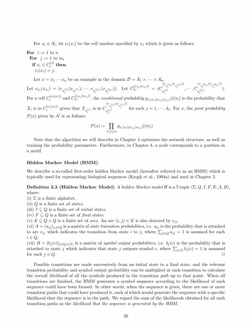
For xi ∈ Xi, let ei(xi) be the cell number specified by xi which is given as follows:

For i := 1 to nFor j := 1 to mi

if xi ∈ C(j)i then

ei(xi) = j.

Let x = x1 · · · xn be an example in the domain D = X1 × · · · × Xn.

Let eπi(xπi

) = (eπ

(1)i

(xπ

(1)i

), · · · , eπ

(ki)i

(xπ

(ki)i

)). Let C(eπi

(xπi))

πi = (C(e

π(1)i

(xπ(1)i

))

π(1)i

, · · · , C(e

π(ki)i

(xπ(ki)i

))

π(ki)i

).

For a cell C(ei(xi))i and C

(eπi(xπi

))πi , the conditional probability pei(xi)|eπi

(xπi)(i|πi) is the probability that

Xi is in C(ei(xi))i given that X

π(j)i

is in C(e

π(j)i

(xπ(j)i

))

π(j)i

for each j = 1, · · · , ki. For x, the joint probability

P (x) given by N is as follows:

P (x) =∏

1≤i≤n

pei(xi)|eπi(xπi

)(i|πi)

Note that the algorithm we will describe in Chapter 4 optimizes the network structure, as well astraining the probability parameters. Furthermore, in Chapter 4, a node corresponds to a position ina motif.

Hidden Markov Model (HMM)

We describe a so-called first-order hidden Markov model (hereafter referred to as an HMM) which istypically used for representing biological sequences (Krogh et al., 1994a) and used in Chapter 5.

Definition 2.3 (Hidden Markov Model) A hidden Markov model H is a 7-tuple 〈Σ, Q, I, F,E,A,B〉,where:(i) Σ is a finite alphabet.(ii) Q is a finite set of states.(iii) I ⊆ Q is a finite set of initial states.(iv) F ⊆ Q is a finite set of final states.(v) E ⊆ Q × Q is a finite set of arcs. An arc (i, j) ∈ E is also denoted by eij .(vi) A = (aij)i,j∈Q is a matrix of state transition probabilities, i.e. aij is the probability that is attachedto arc eij which indicates the transition from state i to j, where

∑

j∈Q aij = 1 is assumed for eachi ∈ Q.(vii) B = (bj(c))j∈Q,c∈Σ is a matrix of symbol output probabilities, i.e. bj(c) is the probability that isattached to state j which indicates that state j outputs symbol c, where

∑

c∈Σ bj(c) = 1 is assumedfor each j ∈ Q. 2

Possible transitions are made successively from an initial state to a final state, and the relevanttransition probability and symbol output probability can be multiplied at each transition to calculatethe overall likelihood of all the symbols produced in the transition path up to that point. When alltransitions are finished, the HMM generates a symbol sequence according to the likelihood of eachsequence could have been formed. In other words, when the sequence is given, there are one or moretransition paths that could have produced it, each of which would generate the sequence with a specificlikelihood that the sequence is in the path. We regard the sum of the likelihoods obtained for all suchtransition paths as the likelihood that the sequence is generated by the HMM.

26

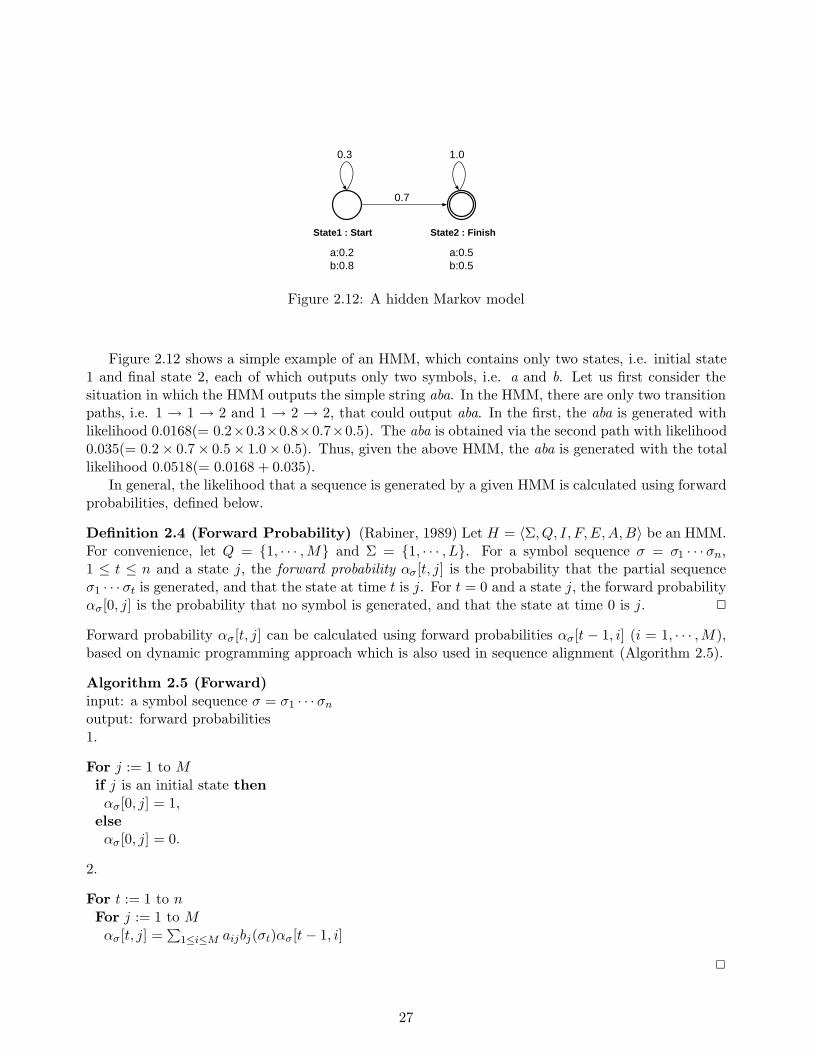
State1 : Start

0.7

a:0.2b:0.8

State2 : Finish

0.3 1.0

a:0.5b:0.5

Figure 2.12: A hidden Markov model

Figure 2.12 shows a simple example of an HMM, which contains only two states, i.e. initial state1 and final state 2, each of which outputs only two symbols, i.e. a and b. Let us first consider thesituation in which the HMM outputs the simple string aba. In the HMM, there are only two transitionpaths, i.e. 1 → 1 → 2 and 1 → 2 → 2, that could output aba. In the first, the aba is generated withlikelihood 0.0168(= 0.2×0.3×0.8×0.7×0.5). The aba is obtained via the second path with likelihood0.035(= 0.2 × 0.7 × 0.5 × 1.0 × 0.5). Thus, given the above HMM, the aba is generated with the totallikelihood 0.0518(= 0.0168 + 0.035).

In general, the likelihood that a sequence is generated by a given HMM is calculated using forwardprobabilities, defined below.

Definition 2.4 (Forward Probability) (Rabiner, 1989) Let H = 〈Σ, Q, I, F,E,A,B〉 be an HMM.For convenience, let Q = {1, · · · ,M} and Σ = {1, · · · , L}. For a symbol sequence σ = σ1 · · · σn,1 ≤ t ≤ n and a state j, the forward probability ασ[t, j] is the probability that the partial sequenceσ1 · · · σt is generated, and that the state at time t is j. For t = 0 and a state j, the forward probabilityασ[0, j] is the probability that no symbol is generated, and that the state at time 0 is j. 2

Forward probability ασ[t, j] can be calculated using forward probabilities ασ[t − 1, i] (i = 1, · · · ,M),based on dynamic programming approach which is also used in sequence alignment (Algorithm 2.5).

Algorithm 2.5 (Forward)input: a symbol sequence σ = σ1 · · · σn

output: forward probabilities1.

For j := 1 to Mif j is an initial state thenασ[0, j] = 1,

elseασ[0, j] = 0.

2.

For t := 1 to nFor j := 1 to Mασ[t, j] =

∑

1≤i≤M aijbj(σt)ασ[t − 1, i]

2

27

N

2

1

State

t-1 t Time

Forward prob. : [t, j]α

3

... ...

1 2 3

......

j

...

σ

Figure 2.13: Forward probability

This iterative operation leads to a lattice structure as shown in Figure 2.13. In the figure,the recursive computation is repeated for each state and time, to obtain the forward probabilityαt(j). From the forward probability ασ[t, j], the likelihood that σ is generated by H, is calculated as∑

1≤i≤M ασ[n, i]βσ [n, i], where βσ[n, i] = 1 if the state i is a final state, and otherwise βσ [n, i] = 0.The problem of learning an HMM is to estimate the state transition probabilities aij (i =

1, · · · ,M, j = 1, · · · ,M) and the symbol output probabilities bj(c) (j = 1, · · · ,M, c = 1, · · · , L) thatmaximize the likelihood of each training sequence. The most general and conventional algorithm tohave been used for the purpose is referred to as the Baum-Welch algorithm, and is a local optimizationalgorithm which will be described in Section 2.2.3. In contrast with this, we propose a new learningalgorithm for HMMs in Chapter 5, which minimizes a kind of error-distance between the real like-lihood that a given training sequence would be generated by an HMM and the target likelihood ofthe sequence. This algorithm allows us to use as training examples not only sequences belonging tothe class to be represented by the HMM but also the sequences which do not, e.g. negative exam-ples. In other words, our method can implement supervised learning of HMMs while the Baum-Welchalgorithm is based exclusively on unsupervised learning.

When a test sequence whose class is unknown is given, we use the HMM that has been trained bythe learning algorithm on a training data set, and parse the input sequence by the trained HMM. Inother words, we search the most likely parse of the input string.

Definition 2.6 (Parse by HMM) Let H = 〈Σ, Q, I, F,E,A,B〉 be an HMM. Let σ be a givensequence, S be a transition path generated by H for σ. Let P (σ,S|H) be the probability that asequence σ is generated by a path S in an HMM H. The most likely parse is given as follows:

arg1 maxS P (σ,S|H)

2

The most likely parse is obtained by replacing ‘∑

’ by ‘max’ in the iterative calculation of the forwardprobability of Algorithm 2.5, and retaining the most likely sub-parse at any intermediate step.

1 The arg maxx f(x) indicates the x which maximizes the f . Similarly, arg minx f(x) is the x which minimizes the f .

28

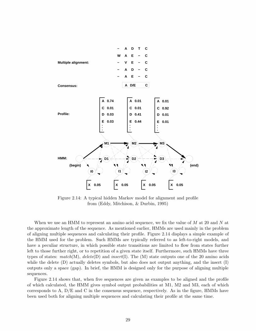
I0 I1 I2 I3

D1 D2 D3

M1 M2 M3

X 0.05 X 0.05 X 0.05 X 0.05

Consensus: A D/E C

(begin) (end)

A D C

A E C

V E C

A D C

A C

T

W −

−

−

−

−

−

−

−E

A

C

D

E...

0.74

0.01

0.03

0.03

A

C

D

E...

0.01

0.01

0.41

0.44

A

C

D

E...

0.01

0.92

0.01

0.01

HMM:

Profile:

Multiple alignment:

Figure 2.14: A typical hidden Markov model for alignment and profilefrom (Eddy, Mitchison, & Durbin, 1995)

When we use an HMM to represent an amino acid sequence, we fix the value of M at 20 and N atthe approximate length of the sequence. As mentioned earlier, HMMs are used mainly in the problemof aligning multiple sequences and calculating their profile. Figure 2.14 displays a simple example ofthe HMM used for the problem. Such HMMs are typically referred to as left-to-right models, andhave a peculiar structure, in which possible state transitions are limited to flow from states furtherleft to those further right, or to repetition of a given state itself. Furthermore, such HMMs have threetypes of states: match(M), delete(D) and insert(I). The (M) state outputs one of the 20 amino acidswhile the delete (D) actually deletes symbols, but also does not output anything, and the insert (I)outputs only a space (gap). In brief, the HMM is designed only for the purpose of aligning multiplesequences.

Figure 2.14 shows that, when five sequences are given as examples to be aligned and the profileof which calculated, the HMM gives symbol output probabilities at M1, M2 and M3, each of whichcorresponds to A, D/E and C in the consensus sequence, respectively. As in the figure, HMMs havebeen used both for aligning multiple sequences and calculating their profile at the same time.

29

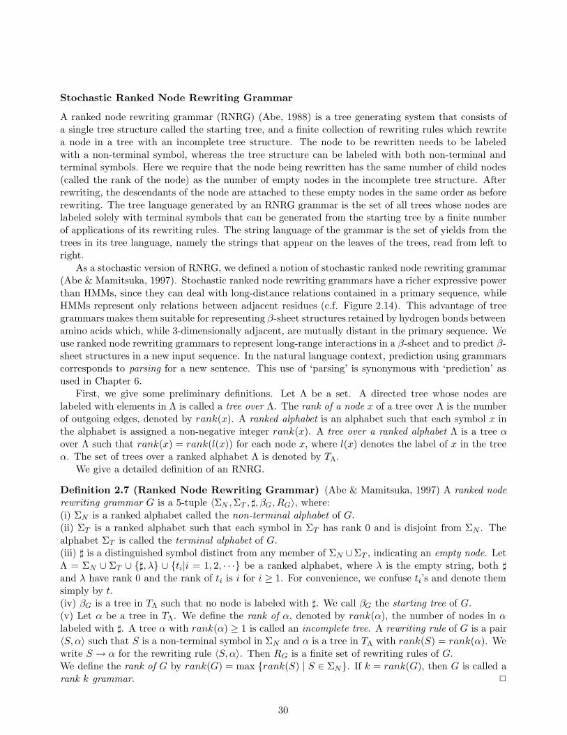
Stochastic Ranked Node Rewriting Grammar

A ranked node rewriting grammar (RNRG) (Abe, 1988) is a tree generating system that consists ofa single tree structure called the starting tree, and a finite collection of rewriting rules which rewritea node in a tree with an incomplete tree structure. The node to be rewritten needs to be labeledwith a non-terminal symbol, whereas the tree structure can be labeled with both non-terminal andterminal symbols. Here we require that the node being rewritten has the same number of child nodes(called the rank of the node) as the number of empty nodes in the incomplete tree structure. Afterrewriting, the descendants of the node are attached to these empty nodes in the same order as beforerewriting. The tree language generated by an RNRG grammar is the set of all trees whose nodes arelabeled solely with terminal symbols that can be generated from the starting tree by a finite numberof applications of its rewriting rules. The string language of the grammar is the set of yields from thetrees in its tree language, namely the strings that appear on the leaves of the trees, read from left toright.

As a stochastic version of RNRG, we defined a notion of stochastic ranked node rewriting grammar(Abe & Mamitsuka, 1997). Stochastic ranked node rewriting grammars have a richer expressive powerthan HMMs, since they can deal with long-distance relations contained in a primary sequence, whileHMMs represent only relations between adjacent residues (c.f. Figure 2.14). This advantage of treegrammars makes them suitable for representing β-sheet structures retained by hydrogen bonds betweenamino acids which, while 3-dimensionally adjacent, are mutually distant in the primary sequence. Weuse ranked node rewriting grammars to represent long-range interactions in a β-sheet and to predict β-sheet structures in a new input sequence. In the natural language context, prediction using grammarscorresponds to parsing for a new sentence. This use of ‘parsing’ is synonymous with ‘prediction’ asused in Chapter 6.

First, we give some preliminary definitions. Let Λ be a set. A directed tree whose nodes arelabeled with elements in Λ is called a tree over Λ. The rank of a node x of a tree over Λ is the numberof outgoing edges, denoted by rank(x). A ranked alphabet is an alphabet such that each symbol x inthe alphabet is assigned a non-negative integer rank(x). A tree over a ranked alphabet Λ is a tree αover Λ such that rank(x) = rank(l(x)) for each node x, where l(x) denotes the label of x in the treeα. The set of trees over a ranked alphabet Λ is denoted by TΛ.

We give a detailed definition of an RNRG.

Definition 2.7 (Ranked Node Rewriting Grammar) (Abe & Mamitsuka, 1997) A ranked noderewriting grammar G is a 5-tuple 〈ΣN ,ΣT , ], βG, RG〉, where:(i) ΣN is a ranked alphabet called the non-terminal alphabet of G.(ii) ΣT is a ranked alphabet such that each symbol in ΣT has rank 0 and is disjoint from ΣN . Thealphabet ΣT is called the terminal alphabet of G.(iii) ] is a distinguished symbol distinct from any member of ΣN ∪ΣT , indicating an empty node. LetΛ = ΣN ∪ ΣT ∪ {], λ} ∪ {ti|i = 1, 2, · · ·} be a ranked alphabet, where λ is the empty string, both ]and λ have rank 0 and the rank of ti is i for i ≥ 1. For convenience, we confuse ti’s and denote themsimply by t.(iv) βG is a tree in TΛ such that no node is labeled with ]. We call βG the starting tree of G.(v) Let α be a tree in TΛ. We define the rank of α, denoted by rank(α), the number of nodes in αlabeled with ]. A tree α with rank(α) ≥ 1 is called an incomplete tree. A rewriting rule of G is a pair〈S, α〉 such that S is a non-terminal symbol in ΣN and α is a tree in TΛ with rank(S) = rank(α). Wewrite S → α for the rewriting rule 〈S, α〉. Then RG is a finite set of rewriting rules of G.We define the rank of G by rank(G) = max {rank(S) | S ∈ ΣN}. If k = rank(G), then G is called arank k grammar. 2

30

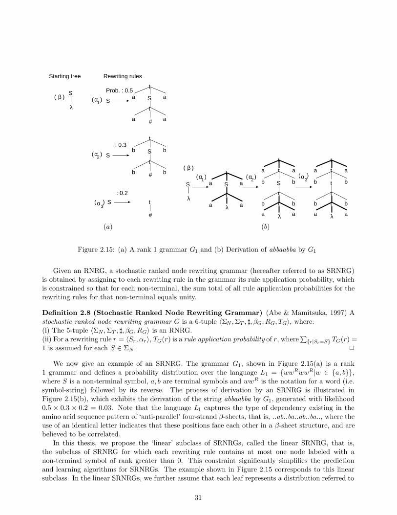
Starting tree

( )

Rewriting rules

S( )

( )

( )

S S

λ

β α

α

α

a a

a a

SSb b

b b

S t

1

2

3

t

t

t

t

Prob. : 0.5

: 0.3

: 0.2

#

#

#

( )

S( ) ( )

S

λ

βα α

a a

a a

Sb b

b b

t1 3

tt

tt

( )α2

a a

t

a a

t

b b

b b

t

t

a a

t

a a

tλ

λ λ

(a) (b)

Figure 2.15: (a) A rank 1 grammar G1 and (b) Derivation of abbaabba by G1

Given an RNRG, a stochastic ranked node rewriting grammar (hereafter referred to as SRNRG)is obtained by assigning to each rewriting rule in the grammar its rule application probability, whichis constrained so that for each non-terminal, the sum total of all rule application probabilities for therewriting rules for that non-terminal equals unity.

Definition 2.8 (Stochastic Ranked Node Rewriting Grammar) (Abe & Mamitsuka, 1997) Astochastic ranked node rewriting grammar G is a 6-tuple 〈ΣN ,ΣT , ], βG, RG, TG〉, where:(i) The 5-tuple 〈ΣN ,ΣT , ], βG, RG〉 is an RNRG.(ii) For a rewriting rule r = 〈Sr, αr〉, TG(r) is a rule application probability of r, where

∑

{r|Sr=S} TG(r) =1 is assumed for each S ∈ ΣN . 2

We now give an example of an SRNRG. The grammar G1, shown in Figure 2.15(a) is a rank1 grammar and defines a probability distribution over the language L1 = {wwRwwR|w ∈ {a, b}},where S is a non-terminal symbol, a, b are terminal symbols and wwR is the notation for a word (i.e.symbol-string) followed by its reverse. The process of derivation by an SRNRG is illustrated inFigure 2.15(b), which exhibits the derivation of the string abbaabba by G1, generated with likelihood0.5 × 0.3 × 0.2 = 0.03. Note that the language L1 captures the type of dependency existing in theamino acid sequence pattern of ‘anti-parallel’ four-strand β-sheets, that is, ..ab..ba..ab..ba.., where theuse of an identical letter indicates that these positions face each other in a β-sheet structure, and arebelieved to be correlated.

In this thesis, we propose the ‘linear’ subclass of SRNRGs, called the linear SRNRG, that is,the subclass of SRNRG for which each rewriting rule contains at most one node labeled with anon-terminal symbol of rank greater than 0. This constraint significantly simplifies the predictionand learning algorithms for SRNRGs. The example shown in Figure 2.15 corresponds to this linearsubclass. In the linear SRNRGs, we further assume that each leaf represents a distribution referred to

31

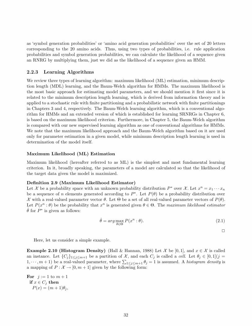
as ‘symbol generation probabilities’ or ‘amino acid generation probabilities’ over the set of 20 letterscorresponding to the 20 amino acids. Thus, using two types of probabilities, i.e. rule applicationprobabilities and symbol generation probabilities, we can calculate the likelihood of a sequence givenan RNRG by multiplying them, just we did as the likelihood of a sequence given an HMM.

2.2.3 Learning Algorithms

We review three types of learning algorithm: maximum likelihood (ML) estimation, minimum descrip-tion length (MDL) learning, and the Baum-Welch algorithm for HMMs. The maximum likelihood isthe most basic approach for estimating model parameters, and we should mention it first since it isrelated to the minimum description length learning, which is derived from information theory and isapplied to a stochastic rule with finite partitioning and a probabilistic network with finite partitioningsin Chapters 3 and 4, respectively. The Baum-Welch learning algorithm, which is a conventional algo-rithm for HMMs and an extended version of which is established for learning SRNRGs in Chapter 6,is based on the maximum likelihood criterion. Furthermore, in Chapter 5, the Baum-Welch algorithmis compared with our new supervised learning algorithm as one of conventional algorithms for HMMs.We note that the maximum likelihood approach and the Baum-Welch algorithm based on it are usedonly for parameter estimation in a given model, while minimum description length learning is used indetermination of the model itself.

Maximum Likelihood (ML) Estimation

Maximum likelihood (hereafter referred to as ML) is the simplest and most fundamental learningcriterion. In it, broadly speaking, the parameters of a model are calculated so that the likelihood ofthe target data given the model is maximized.

Definition 2.9 (Maximum Likelihood Estimator)Let X be a probability space with an unknown probability distribution P ∗ over X . Let xn = x1 · · · xn

be a sequence of n elements generated according to P∗. Let P (θ) be a probability distribution overX with a real-valued parameter vector θ. Let Θ be a set of all real-valued parameter vectors of P (θ).Let P (xn : θ) be the probability that xn is generated given θ ∈ Θ. The maximum likelihood estimatorθ for P ∗ is given as follows:

θ = arg maxθ∈Θ

P (xn : θ). (2.1)

2

Here, let us consider a simple example.

Example 2.10 (Histogram Density) (Hall & Hannan, 1988) Let X be [0, 1], and x ∈ X is calledan instance. Let {Cj}1≤j≤m+1 be a partition of X , and each Cj is called a cell. Let θj ∈ [0, 1](j =1, · · · ,m + 1) be a real-valued parameter, where

∑

1≤j≤m+1 θj = 1 is assumed. A histogram density isa mapping of P : X → [0,m + 1] given by the following form:

For j := 1 to m + 1if x ∈ Cj thenP (x) = (m + 1)θj ,

32

Let ni be the number of examples in the i-th cell Ci. The likelihood of the given examples beingproduced by the parameter values θi (i = 1, · · · ,m + 1) is:

∏

1≤i≤m+1

((m + 1)θi)ni = (m + 1)n

∏

1≤i≤m+1

θni

i , (2.2)

where n =∑

1≤i≤m+1 ni. From Eq. (2.2), the maximum likelihood estimator of θi should be set asfollows:

θi =ni

∑

1≤i≤m+1 ni

=ni

n(i = 1, · · · ,m + 1).

2

Minimum Description Length (MDL) Learning

The minimum description length principle (hereafter referred to as MDL) is derived from the literatureof information theory. Here, first we briefly review the idea behind the MDL principle.

Let us consider a problem in which an encoder A has to communicate with a decorder B. Heresuppose that X = {0, 1}, and xn = x1 · · · xn, a given set of data, is a binary sequence, where xi ∈ X .Here A would like to encode the sequence xn and send it to B assuming no error or noise. Of course,the sequence can be sent with n bits, but A would like to send it with fewer. Under the circumstances,A first encodes the sequence with a probability distribution P for x ∈ X , i.e. P (xn) and sends it to B.Next, A encodes P itself, and then sends it to B. If B receives both messages, B first decodes P andthen obtains xn using it. Therefore, A and B require two processes each for encoding and decoding,respectively, and the best method, which can communicate with the minimum number of bits from Ato B, must minimize the total number of bits that must be processed by the two steps. If encoding Prequires Cn(P ) bits, this requirement is expressed as follows:

minP

{− log P (xn) + Cn(P )}.

This rough idea can be expanded into a principle for estimating an optimal probability distributionfrom n given instances (Rissanen, 1978; Barron & Cover, 1991; Yamanishi, 1992).

We here give some basics of information theory. Let X be a countable set. Let E be a functionE : X → {0, 1}∗. We call E an encoding function and D = E−1 a decoding function. If we encode asequence xn = x1 · · · xn with xi ∈ X (i = 1, · · · , n) into yn = y1 · · · yn with yi = E(xi) (i = 1, · · · , n),then we call x the source sequence, y the code sequence and each yi the codeword. Let l(x) be thelength of E(x), i.e. the number of bits for encoding x by a function E, called a code-length. Letv, w, z ∈ {0, 1}∗. We call v a prefix of w if there is z such that w = vz. A set A ⊆ {0, 1}∗ is prefix-free,if no element in A is the prefix of another element in A. An encoding function E defines a prefix-code,if the set of codewords generated by an encoding function E is prefix-free. Note that when we encodex ∈ X with a prefix-code, the code-length l(x) satisfies the following Kraft inequality (Kraft, 1949):

∑

x∈X2−l(x) ≤ 1.

We define the description length for x ∈ X as the number of bits for encoding x with a prefix-code.Let P be a probability distribution for x ∈ X , where

∑

x∈X P (x) = 1 is assumed. Let L be the averagecodeword length given as L =

∑

x∈X P (x)l(x). We write Lmin for the minimum of L.

33

Theorem 2.11

Lmin ≥ H(P ) =∑

x∈XP (x) log P (x), (2.3)

where Lmin is obtained when l(x) = − log P (x).(Proof)From the following Lagrangian function

L(l(x), P (x)) =∑

x∈XP (x)l(x) + λ(

∑

x∈X2−l(x) − 1),

∑

x∈X P (x)l(x) is minimized when λ = 1ln 2 and l(x) = − log P (x). 2

The theorem indicates that when a probability distribution P for x ∈ X is given, the number of bitsrequired for encoding x with a prefix-code is given as − log P (x).

Definition 2.12 (Minimum Description Length Estimator) (Rissanen, 1978, 1989)Let X be a probability space with an unknown probability distribution P ∗ over X . For simplicity,X is countable. Let xn = x1 · · · xn be a sequence of n elements generated according to P∗. Let Pbe a probability distribution over X . Let H be a set of all probability distributions over X . For asequence xn, the number of bits for encoding xn with a prefix-code is given as − log P (xn). Let Cf

be an encoding function Cf : H → {0, 1}∗, which defines a prefix-code. Let Cn(P ) be the numberof bits for encoding P with a prefix-code defined by Cf , given xn. The minimum description length

estimator P for P ∗ is given as follows:

P = arg minP∈H

{− log P (xn) + Cn(P )}. (2.4)

2

Note that the description length can be divided into two parts in all cases. The MDL principlegiven by Eq. (2.4) can be applied directly to any of the probabilistic models used in various types oflearning problems. When learning using the equation, the first term of the description length indicateshow the model specified by P fits the given examples, and the second term can be regarded as a kindof penalty which depends on the complexity of the model. Therefore, broadly speaking, this principlecan solve the major trade-off in probabilistic models, which arises because simple rules cannot expressgiven training examples exactly and will not achieve good results on test data, while complicated rulesare often weak in accounting for new data though they exactly fit to the training data given. Underthis trade-off, the MDL principle gives us a moderately complex rule with assured optimality, as hasbeen described in the information theory literature. Thus, we can use the MDL principle to optimizethe probabilistic model (i.e. number of parameters) itself, rather than merely to estimate the valuesof probability parameters in the model.

We give an example of calculating the description length of the models to which the MDL principlecan be applied. In this example, we determine the number of cells for the histogram density whichwe described in Definition 2.10, and we here use the notation defined there.

Example 2.13 (Description Length of Histogram Density) (Rissanen, 1989) The first term ofEq. (2.4), which by itself corresponds to the maximum likelihood estimation, is easily derived fromEq. (2.2) as follows :

− log P (xn) = −∑

1≤i≤m+1

ni logni

n− n log(m + 1)

34

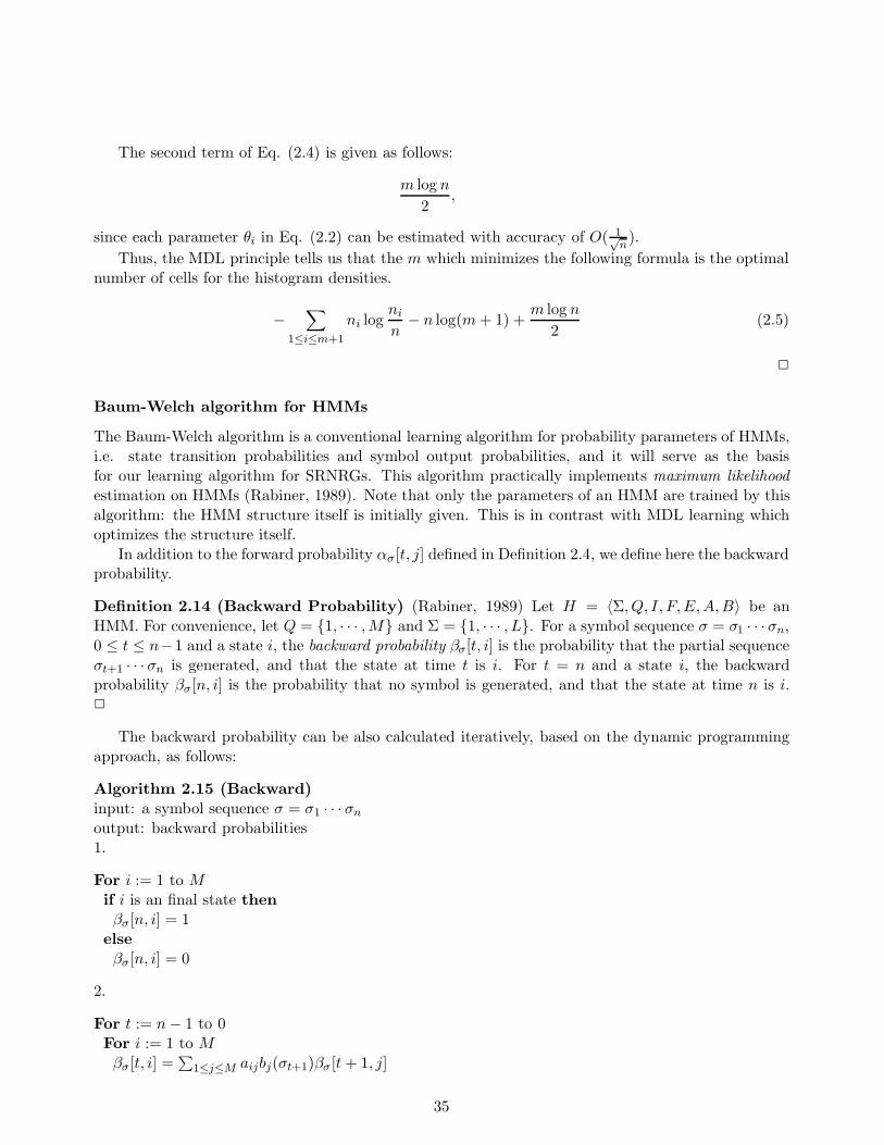
The second term of Eq. (2.4) is given as follows:

m log n

2,

since each parameter θi in Eq. (2.2) can be estimated with accuracy of O( 1√n).

Thus, the MDL principle tells us that the m which minimizes the following formula is the optimalnumber of cells for the histogram densities.

−∑

1≤i≤m+1

ni logni

n− n log(m + 1) +

m log n

2(2.5)

2

Baum-Welch algorithm for HMMs

The Baum-Welch algorithm is a conventional learning algorithm for probability parameters of HMMs,i.e. state transition probabilities and symbol output probabilities, and it will serve as the basisfor our learning algorithm for SRNRGs. This algorithm practically implements maximum likelihoodestimation on HMMs (Rabiner, 1989). Note that only the parameters of an HMM are trained by thisalgorithm: the HMM structure itself is initially given. This is in contrast with MDL learning whichoptimizes the structure itself.

In addition to the forward probability ασ[t, j] defined in Definition 2.4, we define here the backwardprobability.

Definition 2.14 (Backward Probability) (Rabiner, 1989) Let H = 〈Σ, Q, I, F,E,A,B〉 be anHMM. For convenience, let Q = {1, · · · ,M} and Σ = {1, · · · , L}. For a symbol sequence σ = σ1 · · · σn,0 ≤ t ≤ n−1 and a state i, the backward probability βσ[t, i] is the probability that the partial sequenceσt+1 · · · σn is generated, and that the state at time t is i. For t = n and a state i, the backwardprobability βσ[n, i] is the probability that no symbol is generated, and that the state at time n is i.2

The backward probability can be also calculated iteratively, based on the dynamic programmingapproach, as follows:

Algorithm 2.15 (Backward)input: a symbol sequence σ = σ1 · · · σn

output: backward probabilities1.

For i := 1 to Mif i is an final state thenβσ[n, i] = 1

elseβσ[n, i] = 0

2.

For t := n − 1 to 0For i := 1 to Mβσ[t, i] =

∑

1≤j≤M aijbj(σt+1)βσ [t + 1, j]

35

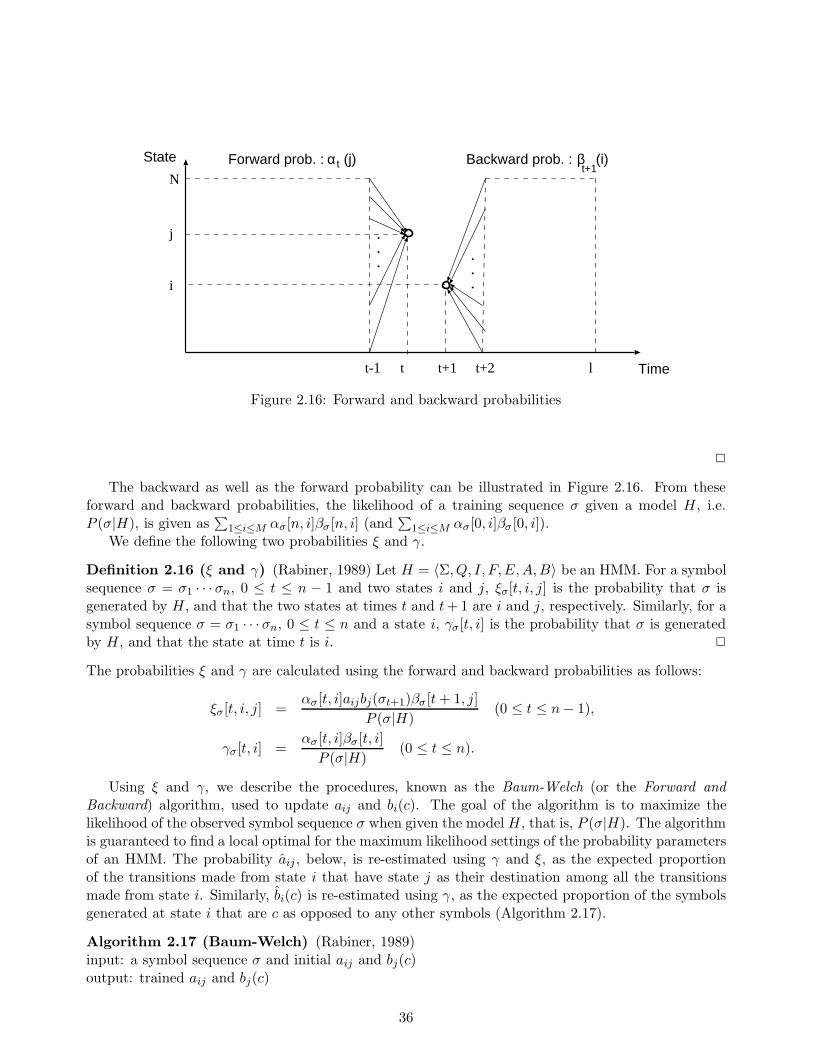
N

j

i

State

t-1 t t+1 l Timet+2

Forward prob. : (j) Backward prob. : (i) t t+1α β

.

.

. ...

Figure 2.16: Forward and backward probabilities

2

The backward as well as the forward probability can be illustrated in Figure 2.16. From theseforward and backward probabilities, the likelihood of a training sequence σ given a model H, i.e.P (σ|H), is given as

∑

1≤i≤M ασ[n, i]βσ [n, i] (and∑

1≤i≤M ασ[0, i]βσ [0, i]).We define the following two probabilities ξ and γ.

Definition 2.16 (ξ and γ) (Rabiner, 1989) Let H = 〈Σ, Q, I, F,E,A,B〉 be an HMM. For a symbolsequence σ = σ1 · · · σn, 0 ≤ t ≤ n − 1 and two states i and j, ξσ[t, i, j] is the probability that σ isgenerated by H, and that the two states at times t and t + 1 are i and j, respectively. Similarly, for asymbol sequence σ = σ1 · · · σn, 0 ≤ t ≤ n and a state i, γσ[t, i] is the probability that σ is generatedby H, and that the state at time t is i. 2

The probabilities ξ and γ are calculated using the forward and backward probabilities as follows:

ξσ[t, i, j] =ασ[t, i]aijbj(σt+1)βσ [t + 1, j]

P (σ|H)(0 ≤ t ≤ n − 1),

γσ[t, i] =ασ[t, i]βσ [t, i]

P (σ|H)(0 ≤ t ≤ n).

Using ξ and γ, we describe the procedures, known as the Baum-Welch (or the Forward andBackward) algorithm, used to update aij and bi(c). The goal of the algorithm is to maximize thelikelihood of the observed symbol sequence σ when given the model H, that is, P (σ|H). The algorithmis guaranteed to find a local optimal for the maximum likelihood settings of the probability parametersof an HMM. The probability aij , below, is re-estimated using γ and ξ, as the expected proportionof the transitions made from state i that have state j as their destination among all the transitionsmade from state i. Similarly, bi(c) is re-estimated using γ, as the expected proportion of the symbolsgenerated at state i that are c as opposed to any other symbols (Algorithm 2.17).

Algorithm 2.17 (Baum-Welch) (Rabiner, 1989)input: a symbol sequence σ and initial aij and bj(c)output: trained aij and bj(c)

36

Repeat the following step until a stopping condition is satisfied, usually until the changes in theprobabilities become smaller than a certain preset amount.1: Re-estimate the aij and bj(c) using training sequences, Eqs. (2.6) and (2.7).

aij =

∑

0≤t≤n−1 ξσ[t, i, j]∑

0≤t≤n−1 γσ[t, i], (2.6)

bi(c) =

∑

1≤t≤n|σt=c γσ[t, i]∑

1≤t≤n γσ[t, i]. (2.7)

2

When more than one symbol sequences are given to be trained, each summation of Eqs. (2.6) and(2.7) is summed over the sequences.

When we apply this algorithm to SRNRGs, the state and transition probability of the HMMs arereplaced with the rewriting rule and rule application probability in the tree grammer, respectively.Furthermore, instead of the symbol output probability in HMMs, the symbol generation probabilitydistribution of each leaf node is used in the algorithm as applied to SRNRGs.

Derivation of the Baum-Welch Re-estimation Algorithm

1. EM Algorithm and Q Function

Let X be a countable set, and let X be a random variable on X . Let Y be a countable set, and let Ybe a random variable on Y. Assume that there exists a mapping y ∈ Y → x ∈ X , and x is observable,but y is not. The x and y are referred to as incomplete data and missing data, respectively, and apair (x, y) is referred to as complete data.

Let P (θ) be a probability distribution with a real-valued parameter vector θ over a probabilityspace. Let Θ be a set of all real-valued parameter vectors. Let f(x|θ) be the likelihood that x isgenerated over θ ∈ Θ. Similarly, let f(x, y|θ) be the likelihood that both x and y are generated overθ ∈ Θ and let f(y|x, θ) be the likelihood that y is generated over θ ∈ Θ given that x is generated.Note the following relation:

f(x|θ) =f(x, y|θ)

f(y|x, θ)

The purpose of the EM (Expectation Maximization) algorithm is to maximize the logarithmiclikelihood log f(x|θ) over θ ∈ Θ.

Taking the conditional expectation over y ∈ Y for the logarithmic likelihood log f(x|Θ), we obtain

log f(x|θ) =∑

y

f(y|x, θ) log f(x, y|θ) −∑

y

f(y|x, θ) log f(y|x, θ). (2.8)

Here, we define the function Q and the function H for parameters θ and θ, as follows:

Definition 2.18 (Q Function and H Function)

Q(θ|θ) =∑

y

f(y|x, θ) log f(x, y|θ) (2.9)

H(θ|θ) =∑

y

f(y|x, θ) log f(y|x, θ)

2

37

Using the definitions, we can rewrite Eq.(2.8) as follows:

log f(x|θ) = Q(θ|θ) − H(θ|θ)

For any two parameters θ and θ, we consider the difference of the logarithmic likelihood,

log f(x|θ) − log f(x|θ) = {Q(θ|θ) − Q(θ|θ)} − {H(θ|θ) − H(θ|θ)}. (2.10)

Here, note that −{H(θ|θ) − H(θ|θ)} ≤ 0 with equality if and only if θ = θ.

Lemma 2.19

−{H(θ|θ) − H(θ|θ)} ≤ 0

(Proof)

H(θ|θ) − H(θ|θ) =∑

y

f(y|x, θ) logf(y|x, θ)

f(y|x, θ)

≤∑

y

f(y|x, θ){f(y|x, θ)

f(y|x, θ)− 1} since log z ≤ z − 1 (0 ≤ z ≤ 1)

=∑

y

f(y|x, θ) −∑

y

f(y|y, θ)

= 0

2

Theorem 2.20 (EM)Q(θ|θ) ≥ Q(θ|θ) ⇒ f(x|θ) ≥ f(x|θ)

(Proof)Using Eq. (2.10) and Lemma 2.19, this theorem holds. 2

This result leads to the following EM algorithm to maximize f(x|θ).

Algorithm 2.21 (EM)input: training dataoutput: trained parameters1. Choose an initial parameter θ and repeat the following steps 2 and 3.2. E-step: Given θ, compute Q(θ|θ).3. M-step: Choose θ = arg maxθ Q(θ|θ), and set θ = θ. 2

2. Hidden Markov Model and Baum-Welch Re-estimation

In hidden Markov models, the x and y correspond to a given symbol sequence and a transition pathof states (i.e. a state sequence), respectively. Let σ = σ1 · · · σn be a given symbol sequence andS = S1 · · ·Sn be a state sequence.

Definition 2.22 (R Function)

R(θ|θ) =∑

S

f(σ, S|θ) log f(σ, S|θ) (2.11)

2

38

Using the definition, we can write Eq.(2.10) as follows:

Q(θ|θ) =1

f(σ|θ)R(θ|θ) (2.12)

Here, let H = 〈Σ, Q, I, F,E,A,B〉 be an HMM. For convenience, let Q = {1, · · · ,M} and Σ ={1, · · · , L}. Then, using the state transition probabilities aij (i = 1, · · · ,M, j = 1, · · · ,M) and symboloutput probabilities bj(c) (j = 1, · · · ,M, c = 1, · · · , L), we can write log f(σ, S|θ) as follows:

log f(σ, S|θ) =∑

1≤t≤n−1

log aStSt+1 +∑

1≤t≤n

log bSt(σt) (2.13)

Substituting Eq. (2.13) into Eq. (2.11), the function R can be seen as follows:

R(θ|θ) =∑

S

f(σ, S|θ)∑

t

log aStSt+1 +∑

S

f(σ, S|θ)∑

t

log bSt(σt)

=∑

S1

· · ·∑

Sn

f(σ, S1, · · · , Sn|θ)∑

t

log aStSt+1 +∑

S1

· · ·∑

Sn

f(σ, S1, · · · , Sn|θ)∑

t

log bSt(σt)

=∑

t

∑

St

∑

St+1

log aStSt+1

∑

S1

· · ·∑

St−1

∑

St+2

· · ·∑

Sn

f(σ, S1, · · · , Sn|θ)

+∑

t

∑

St

log bSt(σt)∑

S1

· · ·∑

St−1

∑

St+1

· · ·∑

Sn

f(σ, S1, · · · , Sn|θ)

=∑

t

∑

i

∑

j

log aij

∑

S1

· · ·∑

St−1

∑

St+2

· · ·∑

Sn

f(σ, S1, · · · , St−1, St = i, St+1 = j, St+1, · · · , Sn|θ)

+∑

t

∑

j

∑

c

log bj(c)∑

S1

· · ·∑

St−1

∑

St+1

· · ·∑

Sn

f(σ, S1, · · · , St−1, St = j, St+1, · · · , Sn|θ)

=∑

i

∑

j

log aij

∑

t

ξσ[t, i, j] +∑

j

∑

c

log bj(c)∑

{t|σt=c}γσ[t, i] (2.14)

Substituting Eq. (2.14) into Eq. (2.12), the function Q can be seen as follows:

Q(θ|θ) =∑

i

∑

j

log aij ·

∑

t ξσ[t, i, j]

f(σ|θ)+

∑

j

∑

c

log bj(c) ·

∑

{t|σt=c} γσ[t, i]

f(σ|θ)(2.15)

From Eq. (2.15), we obtain Eqs. (2.6) and (2.7) in Algorithm 2.17 by choosing θ = arg maxθ Q(θ|θ)in Eq. (2.15).

39

Chapter 3

Predicting α-helices Based onStochastic Rule Learning

3.1 Introduction

Predicting the protein 3-dimensional structure of a given amino acid sequence is the most crucialproblem in the field of computational molecular biology. As such, it has been extensively studied. Inparticular, a number of approaches have been proposed since the 1970s for the problem of predictingprotein secondary structures, which problem is generally placed as the first step to understand theoverall 3-dimensional structure of a given target sequence. These approaches have been applied to thethree-state prediction problem, which is defined as assigning one of the three labels, i.e. α-helix, β-sheetand others, of secondary structures to each of the amino acids in the input sequence. However, theaccuracy in predicting such a problem was at most 70% even in the midst of 1990s, an unsatisfactorylevel for the future purpose of predicting the 3-dimensional structure of a given protein.

These approaches have other disadvantages in addition to the limits of their prediction ability. Inthe feed-forward type neural network frequently used by the methods proposed in the late 1980s orearly 1990s (Qian & Sejnowski, 1988; Kneller et al., 1990; Zhang et al., 1992; Stolorz et al., 1992;Hayward & Collins, 1992), for example, it is difficult for us to find any comprehensive relation betweena region, i.e. a subsequence of amino acids, predicted by the network and the region used for trainingthe network, since such relations are simply represented by numerical weights in the trained network.

On the other hand, Muggleton et al. provided a method for constructing a rule through whichwe can observe relations between a region predicted by a rule and the region used for training therule (Muggleton, King, & Sternberg, 1992). Their rule takes a rough deterministic form, as, forinstance, “in an α-helix, the amino acids at the second position must be large ones, and positiveamino acids must appear at the next position,” etc. This kind of deterministic rule, however, does notalways reflect the actual amino acid distribution at a given position of a secondary structure becausethe categories used for specifying amino acids (e.g. “large”, “positive”, etc.) are not accurate enoughand more exact specification, such as a probability distribution over amino acids, is required.

It is in response to these various drawbacks that we proposed an original method (hereafter referredto simply as the SR method, for stochastic rules) for predicting secondary structures (Mamitsuka& Yamanishi, 1992, 1993, 1995). In this method, we define, as a representation of a probabilitydistribution of amino acids, a stochastic rule for each residue position. In order to learn a stochasticrule, we establish a novel algorithm to optimally categorize twenty amino acids based on the minimumdescription length principle derived from the information theory field, using the physico-chemicalproperties of amino acids themselves, into roughly ten to fifteen groups. We focus on the problem of

40

predicting whether any given region in a sequence is α-helix or not. We call this problem the two-stateprediction problem.

We addressed this particular issue from the following two reasons:

1. Crucial secondary structure.α-helix is the local structure that has been most extensively investigated in biochemistry andhas turned out to be the most crucial among the three states. Thus, predicting α-helices in agiven protein sequence is extremely important in understanding protein structures.

2. Prediction from local properties.While the α-helix is determined to a high degree by local properties alone, such as the short-range interactions of residues, the β-sheet structure, which is another secondary structure tobe predicted in the three-state prediction problem, is significantly affected, as well, by long-range interactions, which extend far beyond the range of local properties. Despite this fact,the secondary structure prediction methods which had been proposed in the same period of theSR method, tried to predict the secondary structures by using the local properties of a givensequence only, and they achieved at most 70% average three-state prediction accuracy. We wantto find out how accurately we could predict secondary structures from the local properties aloneif we limited our prediction to only the α-helix.

We now describe the work of several groups which studied the two-state prediction problem beforeand when we proposed the SR method. Bohr et al. (1988) and Petersen et al. (1990) applied thesame neural network learning method as the Qian and Sejnowski’s method (hereafter referred to asQS) to this problem and achieved 72% prediction accuracy for rhodopsin only. Kneller et al. (1990)studied the problem with a neural network based approach. They achieved 79% average predictionaccuracy for 22 α-domain type proteins, but their test was based on the cross-validation method usingthese proteins, some of which have more than 40% pairwise sequence similarity. In such a datasetin which some two proteins have more than 25% pairwise sequence similarity, secondary structureprediction is required no longer, since existing methods for predicting 3-dimensional structures suchas homology modeling can be practically applied to such a dataset to predict the exact protein 3-dimensional structure of a test sequence. Muggleton et al. (1992) predicted α-helices of α-domaintype proteins using inductive logic programming with 80% average prediction accuracy, but theyused only four proteins as test and the sequence similarities among training and test data were notdescribed. Hayward and Collins (1992) addressed the problem of α-helix prediction with the same dataas those used by Qian and Sejnowski and achieved 78% average accuracy, but the sequence similaritiesamong the data were not clearly stated and the α-helix content in the test sequences was only 28%.Rost and Sander (1993b) (hereafter referred to as RS) also addressed the two-state prediction problemby neural networks using multiple sequence alignment to enhance the training data. They achieved80% prediction accuracy for a dataset in which any test sequence has less than 25% pairwise sequencesimilarity to any training sequence, but they used only α-domain type proteins for test sequences.

In our research, we attempted to predict α-helices in a number of proteins belonging to a widevariety of types, each of which possesses less than 25% pairwise sequence homology to any proteinused for training. We emphasize here that the proteins used by the SR method for prediction were notlimited to α-domain type proteins, while Kneller et al.’s, Muggleton et al.’s and Rost and Sander’smethods were all applied to α-domain type proteins only.

We summarize a number of characteristics of the SR method and our experiments.

1) Probabilistic region prediction.The SR method predicts the probability that a given test region is an α-helix while most conven-tional methods try to predict that a given residue position is in one of three secondary structures,

41

i.e. α-helix, β-sheet and others. We call this probability a likelihood. The idea of region predic-tion was also reported by Presnell et al. (1992) or Lathrop et al. (1987). They predicted localregions using a pattern-matching method.

2) Stochastic rule learning.The relationship between test regions and the two states, i.e. α-helix or not, may be representedby a stochastic rule, which is a probability distribution assigning, to each test region in asequence, a probability that it is in an α-helix.

Furthermore, it is assumed that an individual stochastic rule is represented as the product of anumber of stochastic rules with finite partitioning.

3) Optimal categorization of amino acids with respect to the MDL principle.The SR method allows stochastic rules to make use of any numerical attributes (e.g. physico-chemical characteristics) of amino acids in place of their symbols. Although a number of previ-ously devised methods exist, in which amino acids are categorized on the basis of their numericalattributes (e.g. Taylor, 1986a; Nagano, 1977), such categorization is not theoretically guaranteedto be optimal. The SR method categorizes amino acids for each residue position, on the basisof Rissanen’s minimum description length (MDL) principle, for which its optimality (Rissanen,1978, 1989) and rapid statistical convergence (Yamanishi, 1992) in probabilistic model estima-tion are guaranteed. In addition, we note that until we established the SR method, the MDLprinciple had never been widely applied to probabilistic model estimation, especially in the fieldof computational biology except for the problem of selecting motifs (Yamanishi & Konagaya,1991), to the best of our knowledge.

4) Use of a number of training and test sequences.We use a number of aligned sequences not only for learning stochastic rules for each α-helix butalso for predicting α-helices in a given test sequence. The idea of using a multiple number ofhomologous sequences for training data was used by the SR method (Mamitsuka & Yamanishi,1992) and also by Rost and Sander (1993a, 1993b) in a work independent of ours. They usedsequence profiles in place of twenty discrete amino acid symbols to train neural networks. Fur-thermore, the idea of using test sequences homologous to a given test sequence had not beenemployed by any other method until we established our method, in a similar context, to thebest of our knowledge.

In our experiments, we investigated how well our proposed method predicts α-helices in compari-son with the neural network learning methods, most specifically, the QS method (essentially includingHayward et al.’s method as a special case) and the RS method because the RS was one of the meth-ods (e.g. Rost & Sander, 1993a) which achieved the highest prediction accuracy when we proposedthe SR method and the QS method was the original method from which the RS method was derived.Experimental results show that the SR method achieved an average prediction accuracy of 81% whilethe RS method achieved a prediction accuracy of 80 to 82% depending on its initial values. Thisresult indicates that the SR method reached the same level as that of the RS method, i.e. the highestlevel when we proposed the SR method.

Finally, we briefly explain the progress that has been made in the area of problems in predictingsecondary structures, since we proposed our method. No new method for the two-state predictionproblem has been proposed, to the best of out knowledge. On the other hand, approaches for thethree-state prediction problem have been proposed, and they have slightly improved the predictionaccuracy of the problem to the point where it is no approximately 75% (Frishman & Argos, 1997;

42

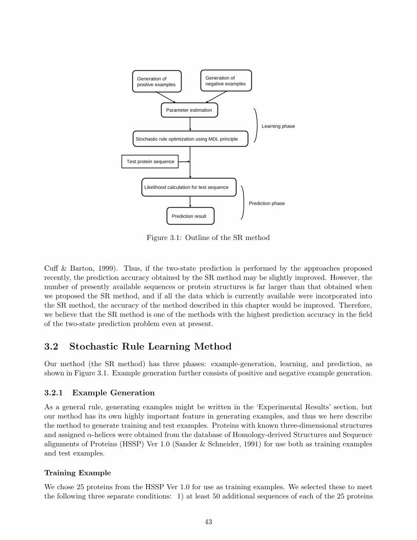
Stochastic rule optimization using MDL principle

Likelihood calculation for test sequence

Prediction result

Generation of positive examples

Generation of negative examples

Test protein sequence

Parameter estimation

Learning phase

Prediction phase

Figure 3.1: Outline of the SR method

Cuff & Barton, 1999). Thus, if the two-state prediction is performed by the approaches proposedrecently, the prediction accuracy obtained by the SR method may be slightly improved. However, thenumber of presently available sequences or protein structures is far larger than that obtained whenwe proposed the SR method, and if all the data which is currently available were incorporated intothe SR method, the accuracy of the method described in this chapter would be improved. Therefore,we believe that the SR method is one of the methods with the highest prediction accuracy in the fieldof the two-state prediction problem even at present.

3.2 Stochastic Rule Learning Method

Our method (the SR method) has three phases: example-generation, learning, and prediction, asshown in Figure 3.1. Example generation further consists of positive and negative example generation.

3.2.1 Example Generation

As a general rule, generating examples might be written in the ‘Experimental Results’ section, butour method has its own highly important feature in generating examples, and thus we here describethe method to generate training and test examples. Proteins with known three-dimensional structuresand assigned α-helices were obtained from the database of Homology-derived Structures and Sequencealignments of Proteins (HSSP) Ver 1.0 (Sander & Schneider, 1991) for use both as training examplesand test examples.

Training Example

We chose 25 proteins from the HSSP Ver 1.0 for use as training examples. We selected these to meetthe following three separate conditions: 1) at least 50 additional sequences of each of the 25 proteins

43

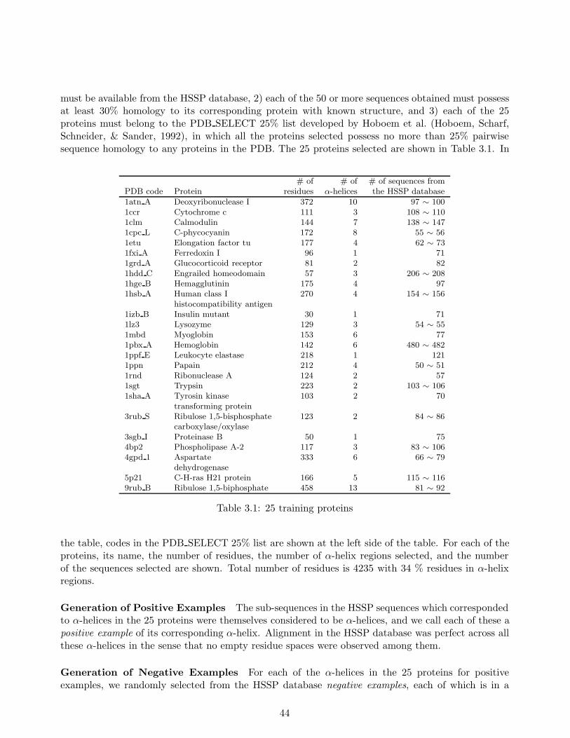
must be available from the HSSP database, 2) each of the 50 or more sequences obtained must possessat least 30% homology to its corresponding protein with known structure, and 3) each of the 25proteins must belong to the PDB SELECT 25% list developed by Hoboem et al. (Hoboem, Scharf,Schneider, & Sander, 1992), in which all the proteins selected possess no more than 25% pairwisesequence homology to any proteins in the PDB. The 25 proteins selected are shown in Table 3.1. In

# of # of # of sequences fromPDB code Protein residues α-helices the HSSP database

1atn A Deoxyribonuclease I 372 10 97 ∼ 1001ccr Cytochrome c 111 3 108 ∼ 1101clm Calmodulin 144 7 138 ∼ 1471cpc L C-phycocyanin 172 8 55 ∼ 561etu Elongation factor tu 177 4 62 ∼ 731fxi A Ferredoxin I 96 1 711grd A Glucocorticoid receptor 81 2 821hdd C Engrailed homeodomain 57 3 206 ∼ 2081hge B Hemagglutinin 175 4 971hsb A Human class I 270 4 154 ∼ 156

histocompatibility antigen1izb B Insulin mutant 30 1 711lz3 Lysozyme 129 3 54 ∼ 551mbd Myoglobin 153 6 771pbx A Hemoglobin 142 6 480 ∼ 4821ppf E Leukocyte elastase 218 1 1211ppn Papain 212 4 50 ∼ 511rnd Ribonuclease A 124 2 571sgt Trypsin 223 2 103 ∼ 1061sha A Tyrosin kinase 103 2 70

transforming protein3rub S Ribulose 1,5-bisphosphate 123 2 84 ∼ 86

carboxylase/oxylase3sgb I Proteinase B 50 1 754bp2 Phospholipase A-2 117 3 83 ∼ 1064gpd 1 Aspartate 333 6 66 ∼ 79

dehydrogenase5p21 C-H-ras H21 protein 166 5 115 ∼ 1169rub B Ribulose 1,5-biphosphate 458 13 81 ∼ 92

Table 3.1: 25 training proteins

the table, codes in the PDB SELECT 25% list are shown at the left side of the table. For each of theproteins, its name, the number of residues, the number of α-helix regions selected, and the numberof the sequences selected are shown. Total number of residues is 4235 with 34 % residues in α-helixregions.

Generation of Positive Examples The sub-sequences in the HSSP sequences which correspondedto α-helices in the 25 proteins were themselves considered to be α-helices, and we call each of these apositive example of its corresponding α-helix. Alignment in the HSSP database was perfect across allthese α-helices in the sense that no empty residue spaces were observed among them.

Generation of Negative Examples For each of the α-helices in the 25 proteins for positiveexamples, we randomly selected from the HSSP database negative examples, each of which is in a

44

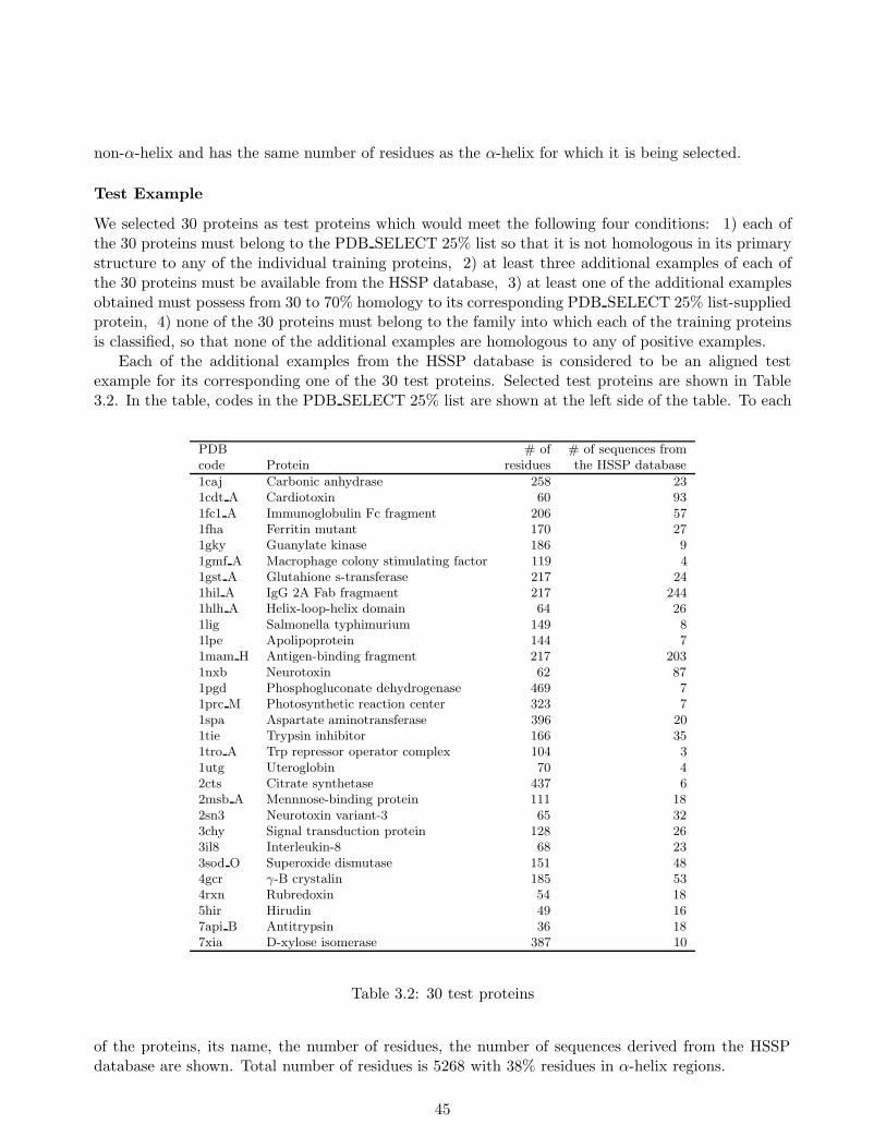
non-α-helix and has the same number of residues as the α-helix for which it is being selected.

Test Example

We selected 30 proteins as test proteins which would meet the following four conditions: 1) each ofthe 30 proteins must belong to the PDB SELECT 25% list so that it is not homologous in its primarystructure to any of the individual training proteins, 2) at least three additional examples of each ofthe 30 proteins must be available from the HSSP database, 3) at least one of the additional examplesobtained must possess from 30 to 70% homology to its corresponding PDB SELECT 25% list-suppliedprotein, 4) none of the 30 proteins must belong to the family into which each of the training proteinsis classified, so that none of the additional examples are homologous to any of positive examples.

Each of the additional examples from the HSSP database is considered to be an aligned testexample for its corresponding one of the 30 test proteins. Selected test proteins are shown in Table3.2. In the table, codes in the PDB SELECT 25% list are shown at the left side of the table. To each

PDB # of # of sequences fromcode Protein residues the HSSP database

1caj Carbonic anhydrase 258 231cdt A Cardiotoxin 60 931fc1 A Immunoglobulin Fc fragment 206 571fha Ferritin mutant 170 271gky Guanylate kinase 186 91gmf A Macrophage colony stimulating factor 119 41gst A Glutahione s-transferase 217 241hil A IgG 2A Fab fragmaent 217 2441hlh A Helix-loop-helix domain 64 261lig Salmonella typhimurium 149 81lpe Apolipoprotein 144 71mam H Antigen-binding fragment 217 2031nxb Neurotoxin 62 871pgd Phosphogluconate dehydrogenase 469 71prc M Photosynthetic reaction center 323 71spa Aspartate aminotransferase 396 201tie Trypsin inhibitor 166 351tro A Trp repressor operator complex 104 31utg Uteroglobin 70 42cts Citrate synthetase 437 62msb A Mennnose-binding protein 111 182sn3 Neurotoxin variant-3 65 323chy Signal transduction protein 128 263il8 Interleukin-8 68 233sod O Superoxide dismutase 151 484gcr γ-B crystalin 185 534rxn Rubredoxin 54 185hir Hirudin 49 167api B Antitrypsin 36 187xia D-xylose isomerase 387 10

Table 3.2: 30 test proteins

of the proteins, its name, the number of residues, the number of sequences derived from the HSSPdatabase are shown. Total number of residues is 5268 with 38% residues in α-helix regions.

45

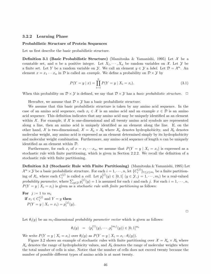
3.2.2 Learning Phase

Probabilistic Structure of Protein Sequences

Let us first describe the basic probabilistic structure.

Definition 3.1 (Basic Probabilistic Structure) (Mamitsuka & Yamanishi, 1995) Let X be acountable set, and n be a positive integer. Let X1, · · · ,Xn be random variables on X . Let Y bea finite set. Let Y be a random variable on Y. We call an element y ∈ Y a label. Let D = Xn. Anelement x = x1 · · · xn in D is called an example. We define a probability on D × Y by

P (Y = y | x) =n

∏

i=1

P (Y = y | Xi = xi). (3.1)

When this probability on D × Y is defined, we say that D × Y has a basic probabilistic structure. 2

Hereafter, we assume that D × Y has a basic probabilistic structure.We assume that this basic probabilistic structure is taken by any amino acid sequence. In the

case of an amino acid sequence, each xi ∈ X is an amino acid and an example x ∈ D is an aminoacid sequence. This definition indicates that any amino acid may be uniquely identified as an elementwithin X . For example, if X is one-dimensional and all twenty amino acid symbols are representedalong a line, then an amino acid is uniquely identified as an element along the line. If, on theother hand, X is two-dimensional, X = Xa × Xb where Xa denotes hydrophobicity, and Xb denotesmolecular weight, any amino acid is expressed as an element determined simply by its hydrophobicityand molecular weight combination. Furthermore, any amino acid sequence of length n can be uniquelyidentified as an element within D.

Furthermore, for each xi of x = x1 · · · xn, we assume that P (Y = y | Xi = xi) is expressed as astochastic rule with finite partitioning, which is given in Section 2.2.2. We recall the definition of astochastic rule with finite partitioning.

Definition 3.2 (Stochastic Rule with Finite Partitioning) (Mamitsuka & Yamanishi, 1995) Let

X n×Y be a basic probabilistic structure. For each i = 1, · · · , n, let {C(j)i }1≤j≤mi

be a finite partition-

ing of Xi, where each C(j)i is called a cell. Let p

(j)i (y) ∈ [0, 1] (y ∈ Y, j = 1, · · · ,mi) be a real-valued

probability parameter, where∑

y∈Y p(j)i (y) = 1 is assumed for each i and each j. For each i = 1, · · · , n,

P (Y = y | Xi = xi) is given as a stochastic rule with finite partitioning as follows:

For j := 1 to mi

if xi ∈ C(j)i and Y = y then

P (Y = y | Xi = xi) = p(j)i (y).

2

Let θi(y) be an mi-dimensional probability parameter vector which is given as follows:

θi(y) = (p(1)i (y), · · · , p

(mi)i (y)) ∈ [0, 1]mi

We write P (Y = y | Xi = xi) over θi(y) as P (Y = y | Xi = xi : θi(y)).Figure 3.2 shows an example of stochastic rules with finite partitioning over X = Xa × Xb where

Xa denotes the range of hydrophobicity values, and Xb denotes the range of molecular weights wherethe total number of cells is nine. Notice that the number of cells does not exceed twenty because thenumber of possible different types of amino acids is at most twenty.

46

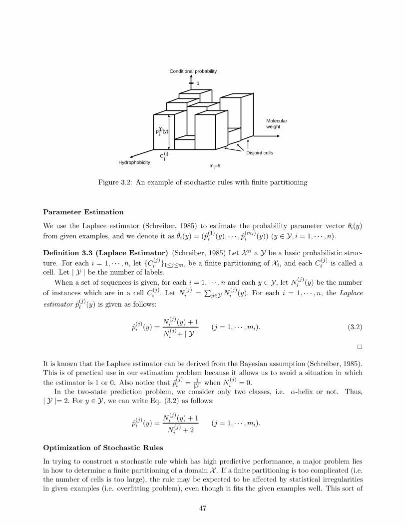
Molecularweight

Hydrophobicity

Conditional probability

1

p (y)i

Disjoint cells

m =9

Ci

i

(j)

(j)

Figure 3.2: An example of stochastic rules with finite partitioning

Parameter Estimation

We use the Laplace estimator (Schreiber, 1985) to estimate the probability parameter vector θi(y)

from given examples, and we denote it as θi(y) = (p(1)i (y), · · · , p

(mi)i (y)) (y ∈ Y, i = 1, · · · , n).

Definition 3.3 (Laplace Estimator) (Schreiber, 1985) Let Xn × Y be a basic probabilistic struc-

ture. For each i = 1, · · · , n, let {C(j)i }1≤j≤mi

be a finite partitioning of Xi, and each C(j)i is called a

cell. Let | Y | be the number of labels.

When a set of sequences is given, for each i = 1, · · · , n and each y ∈ Y, let N(j)i (y) be the number

of instances which are in a cell C(j)i . Let N

(j)i =

∑

y∈Y N(j)i (y). For each i = 1, · · · , n, the Laplace

estimator p(j)i (y) is given as follows:

p(j)i (y) =

N(j)i (y) + 1

N(j)i + | Y |

(j = 1, · · · ,mi). (3.2)

2

It is known that the Laplace estimator can be derived from the Bayesian assumption (Schreiber, 1985).This is of practical use in our estimation problem because it allows us to avoid a situation in which

the estimator is 1 or 0. Also notice that p(j)i = 1

|Y| when N(j)i = 0.

In the two-state prediction problem, we consider only two classes, i.e. α-helix or not. Thus,| Y |= 2. For y ∈ Y, we can write Eq. (3.2) as follows:

p(j)i (y) =

N(j)i (y) + 1

N(j)i + 2

(j = 1, · · · ,mi).

Optimization of Stochastic Rules

In trying to construct a stochastic rule which has high predictive performance, a major problem liesin how to determine a finite partitioning of a domain X . If a finite partitioning is too complicated (i.e.the number of cells is too large), the rule may be expected to be affected by statistical irregularitiesin given examples (i.e. overfitting problem), even though it fits the given examples well. This sort of

47

rule, then, cannot be relied upon to predict α-helices in test examples well. On the other hand, if afinite partitioning is too simple (i.e. the number of the cells is too small), there is a strong likelihoodthat the rule will not learn enough from given examples, and it will be unlikely to perform well withtest examples. In an attempt to determine optimal finite partitioning, so as to avoid both of thesedisadvantageous situations, we determine the optimal number of cells, and the optimal placement ofpartitions.

We establish a new algorithm based on the minimum description length (MDL) principle (Rissanen,1978, 1989) as a criterion to evaluate the optimality of any given structure of a stochastic rule.

As mentioned in Section 2.2.2, the MDL principle says that the optimal finite partitioning is thatwhich minimizes the following two types of description length:

(description length for instances relative to a given rule)

+(description length for the rule itself).

Once a stochastic rule with finite partitioning is constructed, we can calculate the descriptionlength relative to the rule.

The description length for given instances is given as follows:

−∑

1≤j≤mi

∑

y∈YN

(j)i (y) log p

(j)i (y)

The description length for the rule itself can be reduced to the description length of all p(j)i (y).

Notice herelog(N

(j)i

)2 bits are needed to describe each p

(j)i (y), since p

(j)i (y) can be estimated with

accuracy of O( 1√

N(j)i

) (j = 1, · · · ,mi) (see Rissanen, 1989; Yamanishi, 1992). Thus the description

length for the rule itself is calculated as follows:

∑

1≤j≤mi

log N(j)i

2.

Definition 3.4 (Description Length of Stochastic Rule with Finite Partitioning) (Mamitsuka& Yamanishi, 1995) Let Xn × Y be a basic probabilistic structure. For each i = 1, · · · , n, let

{C(j)i }1≤j≤mi

be a finite partitioning of Xi, and each C(j)i is called a cell. For each i = 1, · · · , n, j =

1, · · · ,mi, y ∈ Y, let p(j)i (y) be the Laplace estimator. When a set of sequences is given, for each

i = 1, · · · , n and each y ∈ Y, let N(j)i (y) be the number of instances which are in a cell C

(j)i . Let

N(j)i =

∑

y∈Y N(j)i (y).

For each i = 1, · · · , n, the description length of stochastic rule with finite partitioning is given asfollows:

−∑

1≤j≤mi

∑

y∈YN

(j)i (y) log p

(j)i (y) +

∑

1≤j≤mi

log N(j)i

2. (3.3)

2

The optimal number of cells can be estimated as that which minimizes Eq. (3.3), according to theMDL principle given by Eq. (2.4).

48

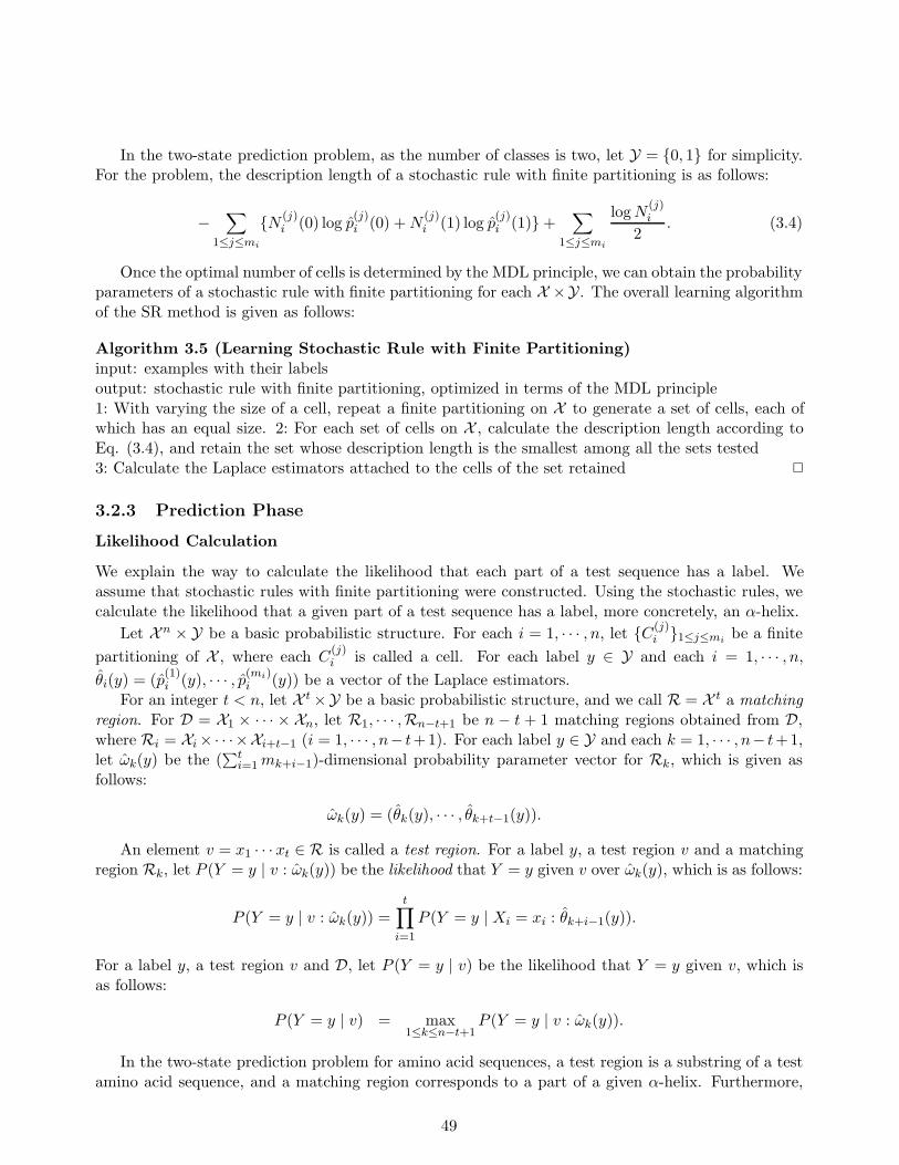
In the two-state prediction problem, as the number of classes is two, let Y = {0, 1} for simplicity.For the problem, the description length of a stochastic rule with finite partitioning is as follows:

−∑

1≤j≤mi

{N(j)i (0) log p

(j)i (0) + N

(j)i (1) log p

(j)i (1)} +

∑

1≤j≤mi

log N(j)i

2. (3.4)

Once the optimal number of cells is determined by the MDL principle, we can obtain the probabilityparameters of a stochastic rule with finite partitioning for each X ×Y. The overall learning algorithmof the SR method is given as follows:

Algorithm 3.5 (Learning Stochastic Rule with Finite Partitioning)input: examples with their labelsoutput: stochastic rule with finite partitioning, optimized in terms of the MDL principle1: With varying the size of a cell, repeat a finite partitioning on X to generate a set of cells, each ofwhich has an equal size. 2: For each set of cells on X , calculate the description length according toEq. (3.4), and retain the set whose description length is the smallest among all the sets tested3: Calculate the Laplace estimators attached to the cells of the set retained 2

3.2.3 Prediction Phase

Likelihood Calculation

We explain the way to calculate the likelihood that each part of a test sequence has a label. Weassume that stochastic rules with finite partitioning were constructed. Using the stochastic rules, wecalculate the likelihood that a given part of a test sequence has a label, more concretely, an α-helix.

Let Xn × Y be a basic probabilistic structure. For each i = 1, · · · , n, let {C(j)i }1≤j≤mi

be a finite

partitioning of X , where each C(j)i is called a cell. For each label y ∈ Y and each i = 1, · · · , n,

θi(y) = (p(1)i (y), · · · , p

(mi)i (y)) be a vector of the Laplace estimators.

For an integer t < n, let X t ×Y be a basic probabilistic structure, and we call R = X t a matchingregion. For D = X1 × · · · × Xn, let R1, · · · ,Rn−t+1 be n − t + 1 matching regions obtained from D,where Ri = Xi ×· · ·×Xi+t−1 (i = 1, · · · , n− t+1). For each label y ∈ Y and each k = 1, · · · , n− t+1,let ωk(y) be the (

∑ti=1 mk+i−1)-dimensional probability parameter vector for Rk, which is given as

follows:

ωk(y) = (θk(y), · · · , θk+t−1(y)).

An element v = x1 · · · xt ∈ R is called a test region. For a label y, a test region v and a matchingregion Rk, let P (Y = y | v : ωk(y)) be the likelihood that Y = y given v over ωk(y), which is as follows:

P (Y = y | v : ωk(y)) =t

∏

i=1

P (Y = y | Xi = xi : θk+i−1(y)).

For a label y, a test region v and D, let P (Y = y | v) be the likelihood that Y = y given v, which isas follows:

P (Y = y | v) = max1≤k≤n−t+1

P (Y = y | v : ωk(y)).

In the two-state prediction problem for amino acid sequences, a test region is a substring of a testamino acid sequence, and a matching region corresponds to a part of a given α-helix. Furthermore,

49

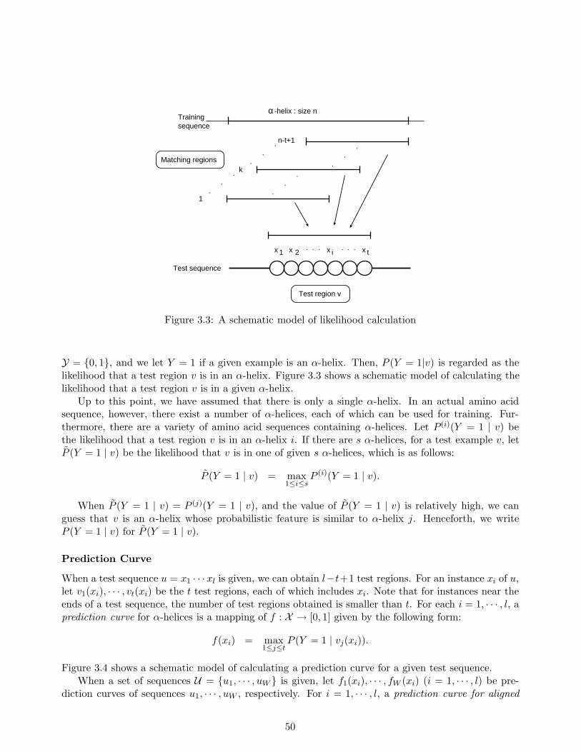
Test sequence

. ..

. ..

. ..

. ..

n-t+1

1

k

x x x x1 2 i t. . . . . .

Test region v

Matching regions

Trainingsequence

-helix : size nα

Figure 3.3: A schematic model of likelihood calculation

Y = {0, 1}, and we let Y = 1 if a given example is an α-helix. Then, P (Y = 1|v) is regarded as thelikelihood that a test region v is in an α-helix. Figure 3.3 shows a schematic model of calculating thelikelihood that a test region v is in a given α-helix.

Up to this point, we have assumed that there is only a single α-helix. In an actual amino acidsequence, however, there exist a number of α-helices, each of which can be used for training. Fur-thermore, there are a variety of amino acid sequences containing α-helices. Let P(i)(Y = 1 | v) bethe likelihood that a test region v is in an α-helix i. If there are s α-helices, for a test example v, letP (Y = 1 | v) be the likelihood that v is in one of given s α-helices, which is as follows:

P (Y = 1 | v) = max1≤i≤s

P (i)(Y = 1 | v).

When P (Y = 1 | v) = P (j)(Y = 1 | v), and the value of P (Y = 1 | v) is relatively high, we canguess that v is an α-helix whose probabilistic feature is similar to α-helix j. Henceforth, we writeP (Y = 1 | v) for P (Y = 1 | v).

Prediction Curve

When a test sequence u = x1 · · · xl is given, we can obtain l−t+1 test regions. For an instance xi of u,let v1(xi), · · · , vt(xi) be the t test regions, each of which includes xi. Note that for instances near theends of a test sequence, the number of test regions obtained is smaller than t. For each i = 1, · · · , l, aprediction curve for α-helices is a mapping of f : X → [0, 1] given by the following form:

f(xi) = max1≤j≤t

P (Y = 1 | vj(xi)).

Figure 3.4 shows a schematic model of calculating a prediction curve for a given test sequence.When a set of sequences U = {u1, · · · , uW } is given, let f1(xi), · · · , fW (xi) (i = 1, · · · , l) be pre-

diction curves of sequences u1, · · · , uW , respectively. For i = 1, · · · , l, a prediction curve for aligned

50

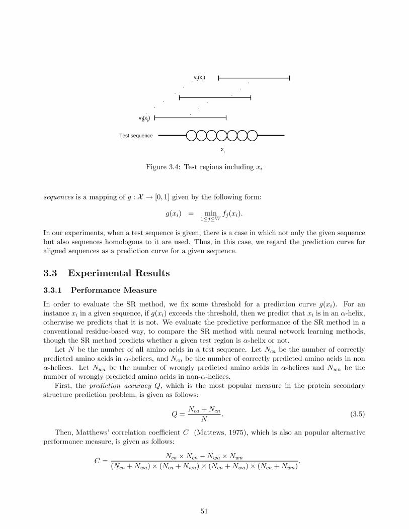
Test sequence

. ..

. ..

. ..

. ..

v (x )

v (x )

x

1

t

i

i

i

Figure 3.4: Test regions including xi

sequences is a mapping of g : X → [0, 1] given by the following form:

g(xi) = min1≤j≤W

fj(xi).

In our experiments, when a test sequence is given, there is a case in which not only the given sequencebut also sequences homologous to it are used. Thus, in this case, we regard the prediction curve foraligned sequences as a prediction curve for a given sequence.

3.3 Experimental Results

3.3.1 Performance Measure

In order to evaluate the SR method, we fix some threshold for a prediction curve g(xi). For aninstance xi in a given sequence, if g(xi) exceeds the threshold, then we predict that xi is in an α-helix,otherwise we predicts that it is not. We evaluate the predictive performance of the SR method in aconventional residue-based way, to compare the SR method with neural network learning methods,though the SR method predicts whether a given test region is α-helix or not.

Let N be the number of all amino acids in a test sequence. Let Nca be the number of correctlypredicted amino acids in α-helices, and Ncn be the number of correctly predicted amino acids in nonα-helices. Let Nwa be the number of wrongly predicted amino acids in α-helices and Nwn be thenumber of wrongly predicted amino acids in non-α-helices.

First, the prediction accuracy Q, which is the most popular measure in the protein secondarystructure prediction problem, is given as follows:

Q =Nca + Ncn

N. (3.5)

Then, Matthews’ correlation coefficient C (Mattews, 1975), which is also an popular alternativeperformance measure, is given as follows:

C =Nca × Ncn − Nwa × Nwn

(Nca + Nwa) × (Nca + Nwn) × (Ncn + Nwa) × (Ncn + Nwn).

51

3.3.2 Stochastic Rule Learning Method

Two types of strategies for the SR method

In our experiments, we used two versions of the SR method: s0 and sMDL.s0 denotes a prediction strategy in which X = XA, which is one-dimensional and represents along

its line the set of all twenty amino acid symbols. Thus, | XA |= 20. In s0, the number of cells specifyinga stochastic rule at each residue position is fixed at twenty, and the structure of the stochastic rule isnot optimized.

sMDL denotes a strategy in which X = XB = Xa × Xb, where Xa denotes the range of hydropho-bicity, and Xb denotes the range of molecular weight. In sMDL, the structure (i.e. the number of cellsand their assignment) of a stochastic rule for each residue position is optimized based on the MDLprinciple. Here we used hydrophobicity values determined by Fauchere and Pliska (1983). Figure 3.5shows an actual example of XB, in which all amino acids belong to a single cell.

40

60

80

100

120

140

160

180

200

R

K

D N

E QH

S

T

P

G

C

Y

A

M

W

V

L

F

I

-1.5 -1 -0.5 0 0.5 1 1.5

Mol

ecul

ar w

eigh

t

Hydrophobicity

Figure 3.5: Domain XB

Size of Test Region

In the prediction phase, we fixed the size of a test region to be seven, since seven amino acids yieldapproximately two turns of an α-helix. Although eight is also a potential candidate for the size, weobserved in preliminary experiments that seven gave better prediction accuracy.

Prediction Accuracy for Training Proteins

The prediction accuracy Q of the SR method depends on the threshold used as the cut-off line forpredicting α-helices. The best average prediction accuracy of s0 and sMDL for 25 training proteinswas 84%, where the threshold was 0.016 or 0.017.

52

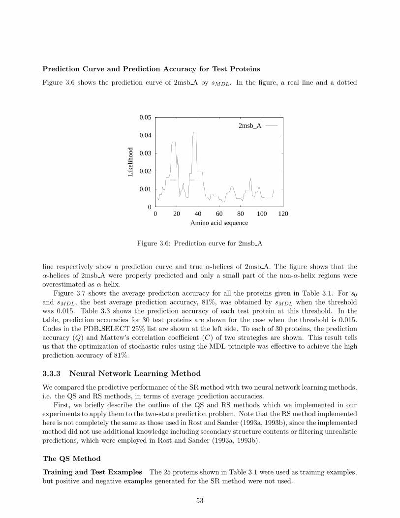
Prediction Curve and Prediction Accuracy for Test Proteins

Figure 3.6 shows the prediction curve of 2msb A by sMDL. In the figure, a real line and a dotted

0

0.01

0.02

0.03

0.04

0.05

0 20 40 60 80 100 120

Lik

elih

ood

Amino acid sequence

2msb_A

Figure 3.6: Prediction curve for 2msb A

line respectively show a prediction curve and true α-helices of 2msb A. The figure shows that theα-helices of 2msb A were properly predicted and only a small part of the non-α-helix regions wereoverestimated as α-helix.

Figure 3.7 shows the average prediction accuracy for all the proteins given in Table 3.1. For s0

and sMDL, the best average prediction accuracy, 81%, was obtained by sMDL when the thresholdwas 0.015. Table 3.3 shows the prediction accuracy of each test protein at this threshold. In thetable, prediction accuracies for 30 test proteins are shown for the case when the threshold is 0.015.Codes in the PDB SELECT 25% list are shown at the left side. To each of 30 proteins, the predictionaccuracy (Q) and Mattew’s correlation coefficient (C) of two strategies are shown. This result tellsus that the optimization of stochastic rules using the MDL principle was effective to achieve the highprediction accuracy of 81%.

3.3.3 Neural Network Learning Method

We compared the predictive performance of the SR method with two neural network learning methods,i.e. the QS and RS methods, in terms of average prediction accuracies.

First, we briefly describe the outline of the QS and RS methods which we implemented in ourexperiments to apply them to the two-state prediction problem. Note that the RS method implementedhere is not completely the same as those used in Rost and Sander (1993a, 1993b), since the implementedmethod did not use additional knowledge including secondary structure contents or filtering unrealisticpredictions, which were employed in Rost and Sander (1993a, 1993b).

The QS Method

Training and Test Examples The 25 proteins shown in Table 3.1 were used as training examples,but positive and negative examples generated for the SR method were not used.

53

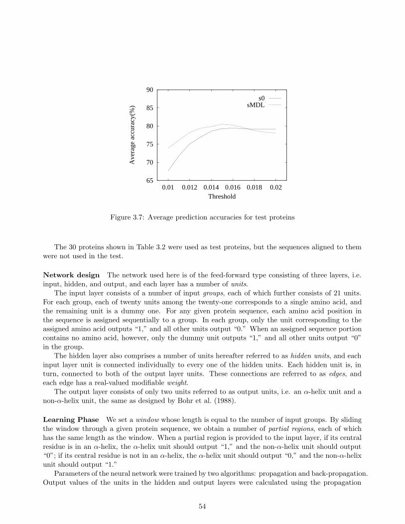
65

70

75

80

85

90

0.01 0.012 0.014 0.016 0.018 0.02

Ave

rage

acc

urac

y(%

)

Threshold

s0sMDL

Figure 3.7: Average prediction accuracies for test proteins

The 30 proteins shown in Table 3.2 were used as test proteins, but the sequences aligned to themwere not used in the test.

Network design The network used here is of the feed-forward type consisting of three layers, i.e.input, hidden, and output, and each layer has a number of units.

The input layer consists of a number of input groups, each of which further consists of 21 units.For each group, each of twenty units among the twenty-one corresponds to a single amino acid, andthe remaining unit is a dummy one. For any given protein sequence, each amino acid position inthe sequence is assigned sequentially to a group. In each group, only the unit corresponding to theassigned amino acid outputs “1,” and all other units output “0.” When an assigned sequence portioncontains no amino acid, however, only the dummy unit outputs “1,” and all other units output “0”in the group.

The hidden layer also comprises a number of units hereafter referred to as hidden units, and eachinput layer unit is connected individually to every one of the hidden units. Each hidden unit is, inturn, connected to both of the output layer units. These connections are referred to as edges, andeach edge has a real-valued modifiable weight.

The output layer consists of only two units referred to as output units, i.e. an α-helix unit and anon-α-helix unit, the same as designed by Bohr et al. (1988).

Learning Phase We set a window whose length is equal to the number of input groups. By slidingthe window through a given protein sequence, we obtain a number of partial regions, each of whichhas the same length as the window. When a partial region is provided to the input layer, if its centralresidue is in an α-helix, the α-helix unit should output “1,” and the non-α-helix unit should output“0”; if its central residue is not in an α-helix, the α-helix unit should output “0,” and the non-α-helixunit should output “1.”

Parameters of the neural network were trained by two algorithms: propagation and back-propagation.Output values of the units in the hidden and output layers were calculated using the propagation

54

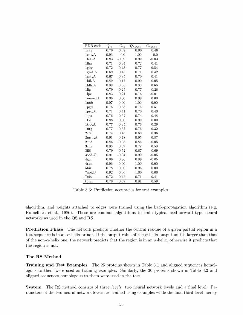
PDB code Qs0Cs0

QsMDLCsMDL

1caj 0.79 0.32 0.90 0.461cdt A 0.93 0.0 1.00 0.01fc1 A 0.83 -0.09 0.92 -0.031fha 0.71 0.34 0.72 0.411gky 0.72 0.43 0.77 0.541gmf A 0.69 0.43 0.71 0.421gst A 0.67 0.35 0.70 0.411hil A 0.89 0.17 0.90 -0.051hlh A 0.89 0.65 0.88 0.661lig 0.79 0.25 0.77 0.281lpe 0.83 0.21 0.76 -0.011mam H 0.96 0.00 0.99 0.001nxb 0.97 0.00 1.00 0.001pgd 0.76 0.53 0.76 0.511prc M 0.71 0.41 0.70 0.401spa 0.76 0.52 0.74 0.481tie 0.88 0.00 0.99 0.001tro A 0.77 0.35 0.76 0.291utg 0.77 0.37 0.76 0.322cts 0.74 0.46 0.69 0.362msb A 0.91 0.78 0.95 0.872sn3 0.86 -0.05 0.86 -0.053chy 0.83 0.67 0.77 0.583il8 0.79 0.52 0.87 0.693sod O 0.91 -0.04 0.90 -0.054gcr 0.86 0.30 0.89 -0.054rxn 0.96 0.00 1.00 0.005hir 0.78 0.00 0.96 0.007api B 0.92 0.00 1.00 0.007xia 0.72 0.45 0.71 0.41

total 0.79 0.57 0.81 0.59

Table 3.3: Prediction accuracies for test examples

algorithm, and weights attached to edges were trained using the back-propagation algorithm (e.g.Rumelhart et al., 1986). These are common algorithms to train typical feed-forward type neuralnetworks as used in the QS and RS.

Prediction Phase The network predicts whether the central residue of a given partial region in atest sequence is in an α-helix or not. If the output value of the α-helix output unit is larger than thatof the non-α-helix one, the network predicts that the region is in an α-helix, otherwise it predicts thatthe region is not.

The RS Method

Training and Test Examples The 25 proteins shown in Table 3.1 and aligned sequences homol-ogous to them were used as training examples. Similarly, the 30 proteins shown in Table 3.2 andaligned sequences homologous to them were used in the test.

System The RS method consists of three levels: two neural network levels and a final level. Pa-rameters of the two neural network levels are trained using examples while the final third level merely

55

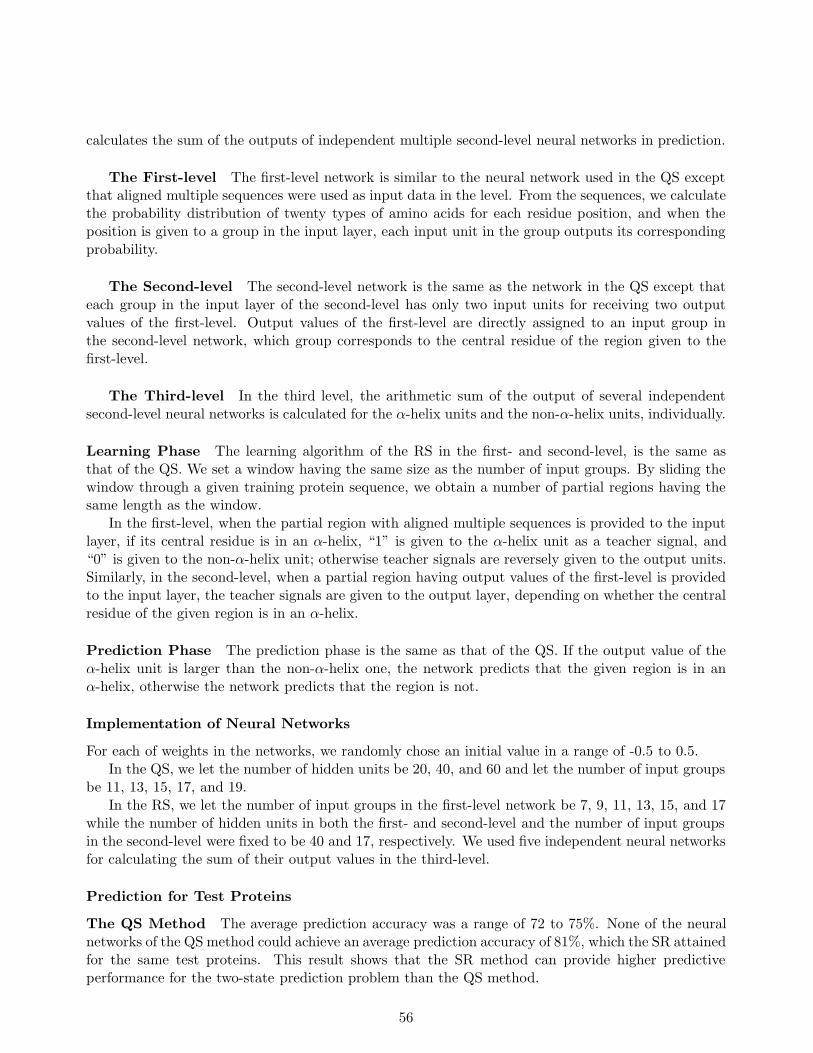
calculates the sum of the outputs of independent multiple second-level neural networks in prediction.

The First-level The first-level network is similar to the neural network used in the QS exceptthat aligned multiple sequences were used as input data in the level. From the sequences, we calculatethe probability distribution of twenty types of amino acids for each residue position, and when theposition is given to a group in the input layer, each input unit in the group outputs its correspondingprobability.

The Second-level The second-level network is the same as the network in the QS except thateach group in the input layer of the second-level has only two input units for receiving two outputvalues of the first-level. Output values of the first-level are directly assigned to an input group inthe second-level network, which group corresponds to the central residue of the region given to thefirst-level.

The Third-level In the third level, the arithmetic sum of the output of several independentsecond-level neural networks is calculated for the α-helix units and the non-α-helix units, individually.

Learning Phase The learning algorithm of the RS in the first- and second-level, is the same asthat of the QS. We set a window having the same size as the number of input groups. By sliding thewindow through a given training protein sequence, we obtain a number of partial regions having thesame length as the window.

In the first-level, when the partial region with aligned multiple sequences is provided to the inputlayer, if its central residue is in an α-helix, “1” is given to the α-helix unit as a teacher signal, and“0” is given to the non-α-helix unit; otherwise teacher signals are reversely given to the output units.Similarly, in the second-level, when a partial region having output values of the first-level is providedto the input layer, the teacher signals are given to the output layer, depending on whether the centralresidue of the given region is in an α-helix.

Prediction Phase The prediction phase is the same as that of the QS. If the output value of theα-helix unit is larger than the non-α-helix one, the network predicts that the given region is in anα-helix, otherwise the network predicts that the region is not.

Implementation of Neural Networks

For each of weights in the networks, we randomly chose an initial value in a range of -0.5 to 0.5.In the QS, we let the number of hidden units be 20, 40, and 60 and let the number of input groups

be 11, 13, 15, 17, and 19.In the RS, we let the number of input groups in the first-level network be 7, 9, 11, 13, 15, and 17

while the number of hidden units in both the first- and second-level and the number of input groupsin the second-level were fixed to be 40 and 17, respectively. We used five independent neural networksfor calculating the sum of their output values in the third-level.

Prediction for Test Proteins

The QS Method The average prediction accuracy was a range of 72 to 75%. None of the neuralnetworks of the QS method could achieve an average prediction accuracy of 81%, which the SR attainedfor the same test proteins. This result shows that the SR method can provide higher predictiveperformance for the two-state prediction problem than the QS method.

56

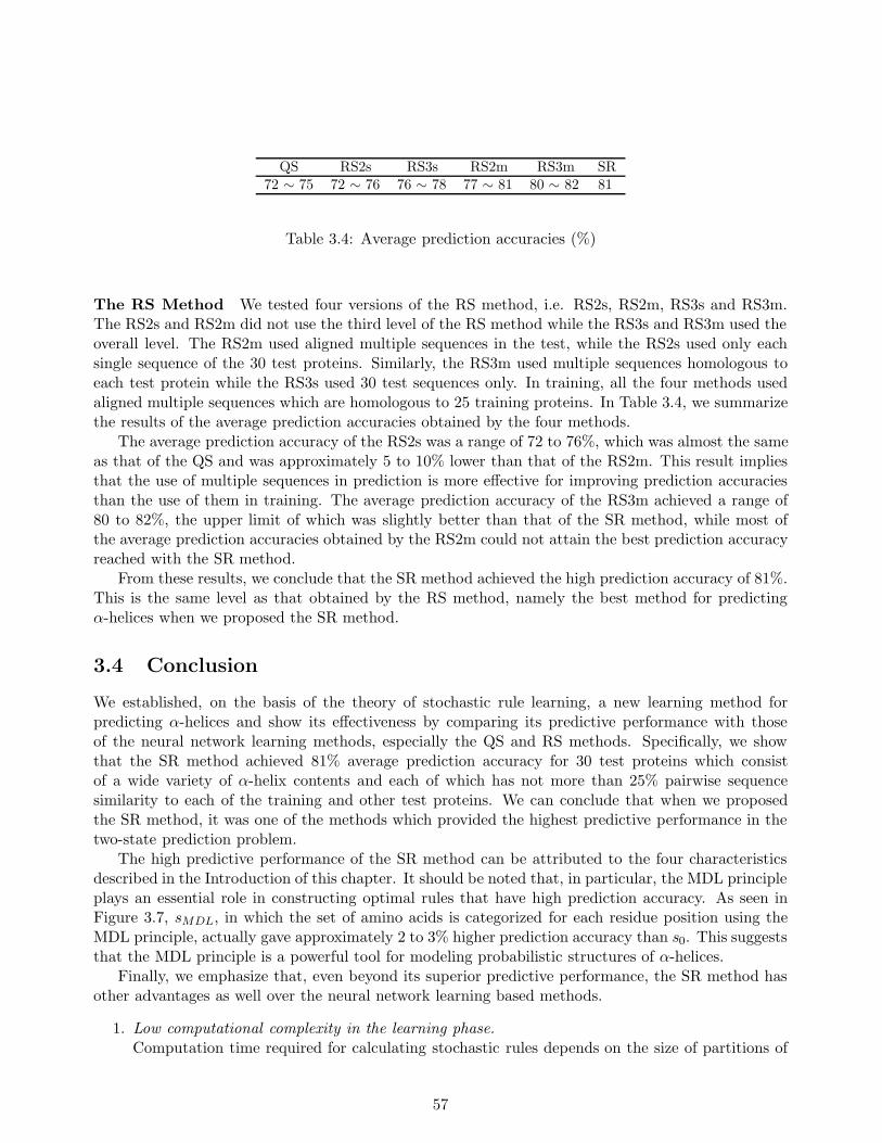
QS RS2s RS3s RS2m RS3m SR72 ∼ 75 72 ∼ 76 76 ∼ 78 77 ∼ 81 80 ∼ 82 81

Table 3.4: Average prediction accuracies (%)

The RS Method We tested four versions of the RS method, i.e. RS2s, RS2m, RS3s and RS3m.The RS2s and RS2m did not use the third level of the RS method while the RS3s and RS3m used theoverall level. The RS2m used aligned multiple sequences in the test, while the RS2s used only eachsingle sequence of the 30 test proteins. Similarly, the RS3m used multiple sequences homologous toeach test protein while the RS3s used 30 test sequences only. In training, all the four methods usedaligned multiple sequences which are homologous to 25 training proteins. In Table 3.4, we summarizethe results of the average prediction accuracies obtained by the four methods.

The average prediction accuracy of the RS2s was a range of 72 to 76%, which was almost the sameas that of the QS and was approximately 5 to 10% lower than that of the RS2m. This result impliesthat the use of multiple sequences in prediction is more effective for improving prediction accuraciesthan the use of them in training. The average prediction accuracy of the RS3m achieved a range of80 to 82%, the upper limit of which was slightly better than that of the SR method, while most ofthe average prediction accuracies obtained by the RS2m could not attain the best prediction accuracyreached with the SR method.

From these results, we conclude that the SR method achieved the high prediction accuracy of 81%.This is the same level as that obtained by the RS method, namely the best method for predictingα-helices when we proposed the SR method.

3.4 Conclusion

We established, on the basis of the theory of stochastic rule learning, a new learning method forpredicting α-helices and show its effectiveness by comparing its predictive performance with thoseof the neural network learning methods, especially the QS and RS methods. Specifically, we showthat the SR method achieved 81% average prediction accuracy for 30 test proteins which consistof a wide variety of α-helix contents and each of which has not more than 25% pairwise sequencesimilarity to each of the training and other test proteins. We can conclude that when we proposedthe SR method, it was one of the methods which provided the highest predictive performance in thetwo-state prediction problem.

The high predictive performance of the SR method can be attributed to the four characteristicsdescribed in the Introduction of this chapter. It should be noted that, in particular, the MDL principleplays an essential role in constructing optimal rules that have high prediction accuracy. As seen inFigure 3.7, sMDL, in which the set of amino acids is categorized for each residue position using theMDL principle, actually gave approximately 2 to 3% higher prediction accuracy than s0. This suggeststhat the MDL principle is a powerful tool for modeling probabilistic structures of α-helices.

Finally, we emphasize that, even beyond its superior predictive performance, the SR method hasother advantages as well over the neural network learning based methods.

1. Low computational complexity in the learning phase.Computation time required for calculating stochastic rules depends on the size of partitions of

57

a domain for a single residue position and the number of given training examples, but it isbasically much less than that required for neural network learning, since the learning phase inthe SR method does not require any iteration as used in the back-propagation algorithm. In ourexperiments, the computation time for stochastic rule learning was less than one tenth of thatfor neural network learning.

2. Comprehensibility of physico-chemical properties of α-helix.The SR method can tell us which α-helix in training proteins has the same type of physico-chemical properties as the predicted α-helix. We cannot expect neural network learning methods,such as the QS and RS methods, to provide this kind of analysis.

58

Chapter 4

Representing Inter-residue Relationswith Probabilistic Networks

4.1 Introduction

Motifs are generally functionally crucial patterns hidden in amino acid sequences, and the mostimportant theme related to motifs is to represent them in some form which can be searched forin new sequences with reasonable accuracy and speed. A motif has been represented simply by asequence pattern as used in the PROSITE database (Hofmann et al., 1999), or by a profile whichcorresponds to probability distributions of amino acids (Luthy et al., 1994; Gribskov et al., 1990). Allthese simple approaches for representing a motif provide us with only 1-dimensional information onthe motif, whereas the motif is expected to include remote inter-residue relations because its functionis affected by interactions between residues which are three-dimensionally adjacent to each other butmay be distant on the one-dimensional level. If we could extract such inter-residue relations within amotif and at the same time automatically display the relations in some visible form, the result wouldbe a great aid in elucidating mechanisms related to the motif. A hidden Markov model (HMM), whichwas proposed to represent a profile or a motif, attempts to deal with such an inter-residue relation asa probability (Krogh et al., 1994a; Baldi et al., 1994). That is, a transition probability between twostates in an HMM represents the probabilistic relation between two adjacent residues. Although anHMM can be trained by sequences with a variety of lengths, the structure of an HMM used in generalis fixed as a model, in which only transitions between adjacent states are allowed. Thus such an HMMdoes not represent any relations between distant residues, i.e. remote inter-residue relations.

Motivated largely by these drawbacks, we focused on non-adjacent inter-residue relations andestablished a new method for automatically constructing networks to represent such relations, withina very short period of time (Mamitsuka, 1993, 1995). Our method constructs, from a number ofaligned sequences for a short sequence, a probabilistic network, in which each node corresponds to aresidue in the sequence, and a directed arc between nodes represents a probabilistic relation betweenthe corresponding residues, i.e. a probabilistic inter-residue relation. Furthermore, a finite partitioningis done over a domain corresponding to a node, and thus we call our network the probabilistic networkwith finite partitionings. For simplicity, hereafter we refer to it as a probabilistic network in thisIntroduction. The idea behind our method for detecting probabilistic inter-residue relations hiddenin given sequences is very simple: Several positions in a given sequence are said to have an inter-residue relation if substitutions in all of those positions in the sequences aligned to the sequenceco-occur while such substitutions are not found in other positions. We quantify the strength of theinter-residue relation as a conditional probability in the probabilistic network.

59

We established a time-efficient algorithm to learn these probabilistic inter-residue relations, basedon the minimum description length (MDL) principle (Rissanen, 1978, 1989) and a greedy algorithm.The MDL principle gives us a criterion to obtain the optimal probabilistic network using given data,and the greedy algorithm enables the network to be obtained efficiently in terms of computation time.We emphasize that we had to devise our algorithm to employ them, because there exist exponentialcombinations of all possible network structures. Under the circumstance, we divide our whole prob-abilistic network into partial probabilistic networks, each of which has a node and its predecessors,from each of which a directed arc goes to the node. This division gives us two merits. By doingthis, first, the description length of a whole network is the sum of the description lengths of all par-tial probabilistic networks. Second, based on this, if we obtain the optimal probabilistic networkwith respect to the MDL principle, we merely have to search, in each partial probabilistic network,for predecessors which reduce the description length of the partial network by the largest amount.However, even for a partial network, there exist exponential combinations of predecessors, and thereexists a no-cycle constraint in the directed acyclic graph of our probabilistic network. That is, thenext problem is how to search efficiently for predecessors for each partial network among all possiblecombinations satisfying the no-cycle constraint. Thus, we use a greedy algorithm, which for a wholenetwork iteratively chooses a predecessor which reduces the description length by the largest amountamong all possible candidates which do not violate the no-cycle constraint. It should be noted that thedescription length criterion we use can be calculated efficiently in terms of computation time. Cooperand Herskovits (1992) used a similar greedy algorithm for searching for the optimal structure of aprobabilistic network, but their method requires a great deal of time (i.e. a day or more) to calculatethe criterion to determine whether a network is being improved or not when a new arc is added to thenetwork. In contrast, our description length criterion can be calculated in a much shorter time (i.e.within a second).

In our experiments, we focused on a loop region of the EF-hand motif, which is peculiar tocalcium binding proteins (Moncrief et al., 1990; Nakayama et al., 1992), and obtained actual aminoacid sequences of the region. Experimental results show that our method constructed a probabilisticnetwork for the region using the given sequences within a single second, and the network capturedseveral important three-dimensional features of the region. From these results, we conclude that ourmethod can provide crucial information for analyzing protein sequences.

Before we proposed our method, two other groups also tried to apply this type of probabilisticnetworks to represent an amino acid sequence. Delcher et al. (1993) used a probabilistic network (tree)for a protein secondary structure prediction problem. They, however, used a network with a fixedstructure that did not provide any information on distant residues. Klingler and Brutlag (1994) alsoused a probabilistic network for representing correlations between residue positions. They capturedsome characteristics of α-helices which are generally known, though their method deals with onlycorrelations between residue pairs. We emphasize that our method directly deals with relationsamong more than two residues, and automatically constructs a near-optimal network with respectto the MDL principle.

Since we proposed our method, no probabilistic networks have been applied to represent biologicalsequences, to the best of our knowledge. This is because HMMs, which as mentioned earlier arewell suited for capturing a profile in given sequences with variable lengths, have been proven to beuseful for several problems in biological sequence analysis (Durbin et al., 1998) and HMMs are nowgenerally used as stochastic knowledge representations in the computational biology field. However,probabilistic networks themselves are even now widely applied to represent uncertain knowledge ina variety of other fields, and thus methods for learning or modifying them are now still extensivelystudied in one field of artificial intelligence (Langley, Provan, & Smyth, 1997). Here, it is worth noting

60

that one disadvantage of most of the methods is that they require a large amount of computationtime to calculate the optimal probabilistic network, (e.g. Heckerman, Geiger, & Chickering, 1995).In contrast, as mentioned earlier, our method allows us to calculate a near-optimal network veryefficiently in terms of computation time. From this viewpoint, our method is still useful for learninga near-optimal probabilistic network in a limited period of time.

4.2 Method

4.2.1 Probabilistic Network with Finite Partitionings

We recall the definition of probabilistic network with finite partitionings, which is given in Chapter 2.Let K = (S,A) be a directed acyclic graph with the node set S = {1, · · · , n} and the arc set A.

If i → j is an arc, we say that i is a predecessor of j. Let πi = {π(1)i , · · · , π

(ki)i } ⊂ S be the set of the

predecessors of node i. Note that i /∈ πi.

Definition 4.1 (Probabilistic Network with Finite Partitionings) (Mamitsuka, 1995) A prob-abilistic network with finite partitionings N consists of the following:(i) A directed acyclic graph K = (S,A).(ii) Random variables Xi on domains Xi for i = 1, · · · , n.

(iii) A finite partitioning {C(j)i }1≤j≤mi

of Xi for each i = 1, · · · , n. 2

Let V = {X1, · · · ,Xn}.For a variable Xi, we define the set of predecessor variables Πi = {X

π(1)i

, · · · ,Xπ

(ki)i

} ⊂ V.

For xi ∈ Xi, let ei(xi) be the cell number specified by xi which is given as follows:

For i := 1 to nFor j := 1 to mi

if xi ∈ C(j)i then

ei(xi) = j.

Let x = x1 · · · xn be an example in the domain D = X1 × · · · × Xn.

Let eπi(xπi

) = (eπ

(1)i

(xπ

(1)i

), · · · , eπ

(ki)i

(xπ

(ki)i

)). Let C(eπi

(xπi))

πi = (C(e

π(1)i

(xπ(1)i

))

π(1)i

, · · · , C(e

π(ki)i

(xπ(ki)i

))

π(ki)i

).

For a cell C(ei(xi))i and C

(eπi(xπi

))πi , the conditional probability pei(xi)|eπi

(xπi)(i|πi) is the probability that

Xi is in C(ei(xi))i given that X

π(j)i

is in C(e

π(j)i

(xπ(j)i

))

π(j)i

for each j = 1, · · · , ki. For x, the joint probability

P (x) given by N is as follows:

P (x) =∏

1≤i≤n

pei(xi)|eπi(xπi

)(i|πi) (4.1)

4.2.2 Efficient MDL Learning Algorithm for Probabilistic Networks

Optimal Finite Partitioning with the MDL Principle

The main purpose of a finite partitioning is to cut down on the computational requirement in cal-culating the description length of a probabilistic network with finite partitionings. Another possibleadvantage of a finite partitioning is to improve the predictive performance of a network, when thenetwork is trained by a number of sequences belonging to a class and an unknown sequence is given to

61

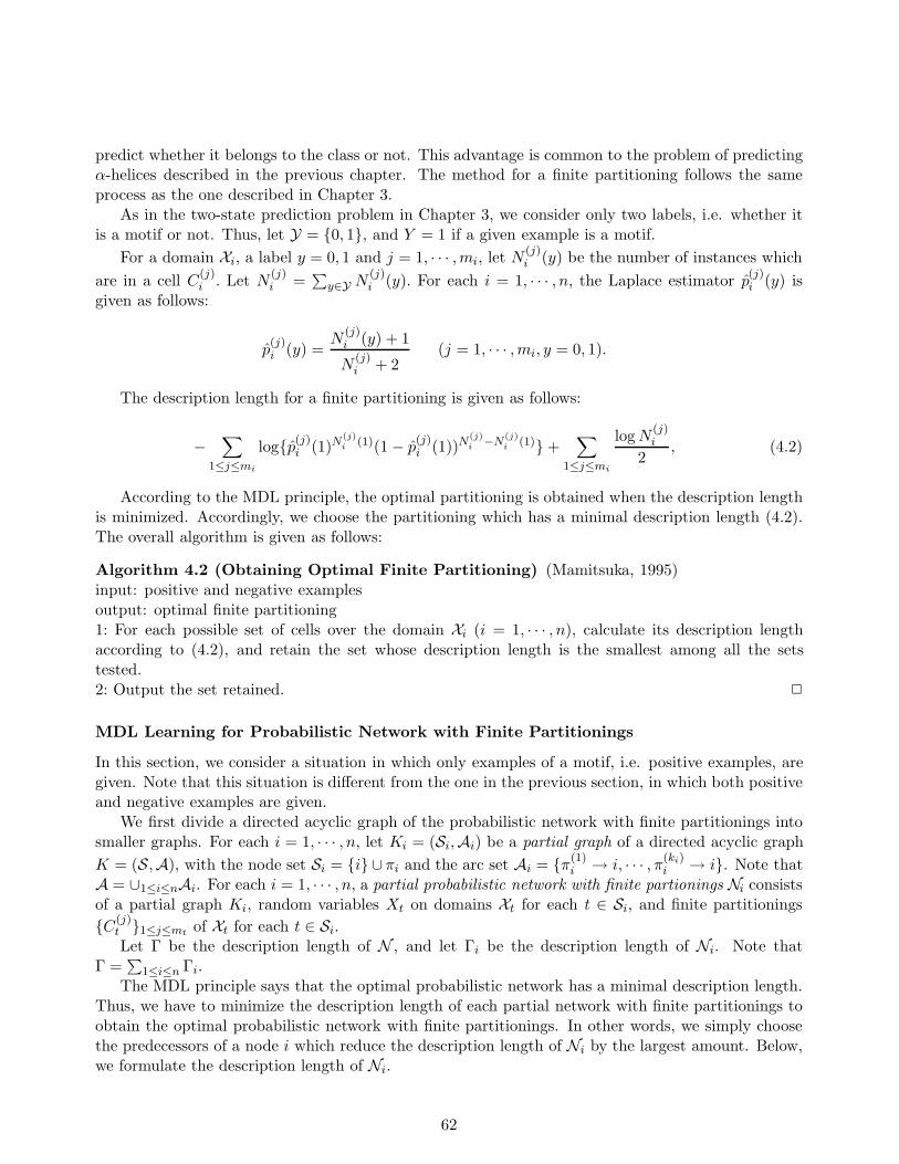
predict whether it belongs to the class or not. This advantage is common to the problem of predictingα-helices described in the previous chapter. The method for a finite partitioning follows the sameprocess as the one described in Chapter 3.

As in the two-state prediction problem in Chapter 3, we consider only two labels, i.e. whether itis a motif or not. Thus, let Y = {0, 1}, and Y = 1 if a given example is a motif.

For a domain Xi, a label y = 0, 1 and j = 1, · · · ,mi, let N(j)i (y) be the number of instances which

are in a cell C(j)i . Let N

(j)i =

∑

y∈Y N(j)i (y). For each i = 1, · · · , n, the Laplace estimator p

(j)i (y) is

given as follows:

p(j)i (y) =

N(j)i (y) + 1

N(j)i + 2

(j = 1, · · · ,mi, y = 0, 1).

The description length for a finite partitioning is given as follows:

−∑

1≤j≤mi

log{p(j)i (1)N

(j)i

(1)(1 − p(j)i (1))N

(j)i

−N(j)i

(1)} +∑

1≤j≤mi

log N(j)i

2, (4.2)

According to the MDL principle, the optimal partitioning is obtained when the description lengthis minimized. Accordingly, we choose the partitioning which has a minimal description length (4.2).The overall algorithm is given as follows:

Algorithm 4.2 (Obtaining Optimal Finite Partitioning) (Mamitsuka, 1995)input: positive and negative examplesoutput: optimal finite partitioning1: For each possible set of cells over the domain Xi (i = 1, · · · , n), calculate its description lengthaccording to (4.2), and retain the set whose description length is the smallest among all the setstested.2: Output the set retained. 2

MDL Learning for Probabilistic Network with Finite Partitionings

In this section, we consider a situation in which only examples of a motif, i.e. positive examples, aregiven. Note that this situation is different from the one in the previous section, in which both positiveand negative examples are given.

We first divide a directed acyclic graph of the probabilistic network with finite partitionings intosmaller graphs. For each i = 1, · · · , n, let Ki = (Si,Ai) be a partial graph of a directed acyclic graph

K = (S,A), with the node set Si = {i} ∪ πi and the arc set Ai = {π(1)i → i, · · · , π

(ki)i → i}. Note that

A = ∪1≤i≤nAi. For each i = 1, · · · , n, a partial probabilistic network with finite partionings Ni consistsof a partial graph Ki, random variables Xt on domains Xt for each t ∈ Si, and finite partitionings

{C(j)t }1≤j≤mt of Xt for each t ∈ Si.Let Γ be the description length of N , and let Γi be the description length of Ni. Note that

Γ =∑

1≤i≤n Γi.The MDL principle says that the optimal probabilistic network has a minimal description length.

Thus, we have to minimize the description length of each partial network with finite partitionings toobtain the optimal probabilistic network with finite partitionings. In other words, we simply choosethe predecessors of a node i which reduce the description length of Ni by the largest amount. Below,we formulate the description length of Ni.

62

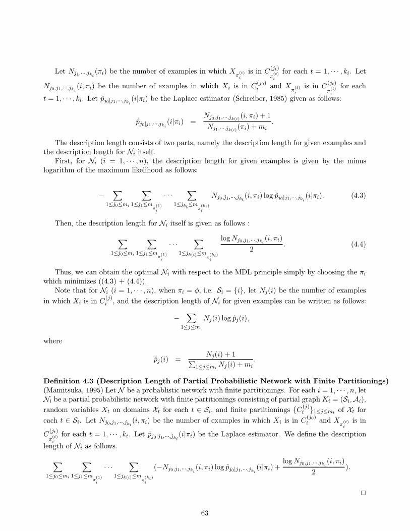
Let Nj1,···,jki(πi) be the number of examples in which X

π(t)i

is in C(jt)

π(t)i

for each t = 1, · · · , ki. Let

Nj0,j1,···,jki(i, πi) be the number of examples in which Xi is in C

(j0)i and X

π(t)i

is in C(jt)

π(t)i

for each

t = 1, · · · , ki. Let pj0|j1,···,jki(i|πi) be the Laplace estimator (Schreiber, 1985) given as follows:

pj0|j1,···,jki(i|πi) =

Nj0,j1,···,jk(i)(i, πi) + 1

Nj1,···,jk(i)(πi) + mi

.

The description length consists of two parts, namely the description length for given examples andthe description length for Ni itself.

First, for Ni (i = 1, · · · , n), the description length for given examples is given by the minuslogarithm of the maximum likelihood as follows:

−∑

1≤j0≤mi

∑

1≤j1≤mπ(1)i

· · ·∑

1≤jki≤m

π(ki)i

Nj0,j1,···,jki(i, πi) log pj0|j1,···,jki

(i|πi). (4.3)

Then, the description length for Ni itself is given as follows :

∑

1≤j0≤mi

∑

1≤j1≤mπ(1)i

· · ·∑

1≤jk(i)≤mπ(ki)i

log Nj0,j1,···,jki(i, πi)

2. (4.4)

Thus, we can obtain the optimal Ni with respect to the MDL principle simply by choosing the πi

which minimizes ((4.3) + (4.4)).Note that for Ni (i = 1, · · · , n), when πi = φ, i.e. Si = {i}, let Nj(i) be the number of examples

in which Xi is in C(j)i , and the description length of Ni for given examples can be written as follows:

−∑

1≤j≤mi

Nj(i) log pj(i),

where

pj(i) =Nj(i) + 1

∑

1≤j≤miNj(i) + mi

.

Definition 4.3 (Description Length of Partial Probabilistic Network with Finite Partitionings)(Mamitsuka, 1995) Let N be a probablistic network with finite partitionings. For each i = 1, · · · , n, letNi be a partial probabilistic network with finite partitionings consisting of partial graph Ki = (Si,Ai),

random variables Xt on domains Xt for each t ∈ Si, and finite partitionings {C(j)t }1≤j≤mt of Xt for

each t ∈ Si. Let Nj0,j1,···,jki(i, πi) be the number of examples in which Xi is in C

(j0)i and X

π(t)i

is in

C(jt)

π(t)i

for each t = 1, · · · , ki. Let pj0|j1,···,jki(i|πi) be the Laplace estimator. We define the description

length of Ni as follows.

∑

1≤j0≤mi

∑

1≤j1≤mπ(1)i

· · ·∑

1≤jk(i)≤mπ(ki)i

(−Nj0,j1,···,jki(i, πi) log pj0|j1,···,jki

(i|πi) +log Nj0,j1,···,jki

(i, πi)

2).

2

63

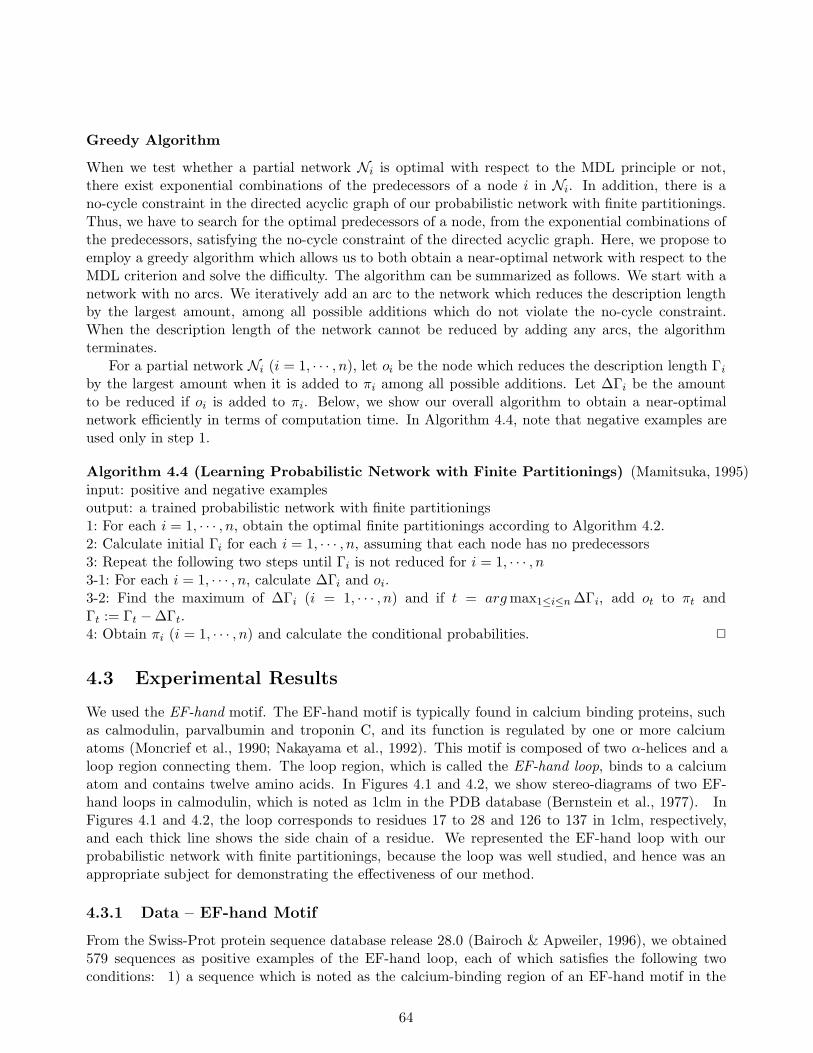
Greedy Algorithm

When we test whether a partial network Ni is optimal with respect to the MDL principle or not,there exist exponential combinations of the predecessors of a node i in Ni. In addition, there is ano-cycle constraint in the directed acyclic graph of our probabilistic network with finite partitionings.Thus, we have to search for the optimal predecessors of a node, from the exponential combinations ofthe predecessors, satisfying the no-cycle constraint of the directed acyclic graph. Here, we propose toemploy a greedy algorithm which allows us to both obtain a near-optimal network with respect to theMDL criterion and solve the difficulty. The algorithm can be summarized as follows. We start with anetwork with no arcs. We iteratively add an arc to the network which reduces the description lengthby the largest amount, among all possible additions which do not violate the no-cycle constraint.When the description length of the network cannot be reduced by adding any arcs, the algorithmterminates.

For a partial network Ni (i = 1, · · · , n), let oi be the node which reduces the description length Γi

by the largest amount when it is added to πi among all possible additions. Let ∆Γi be the amountto be reduced if oi is added to πi. Below, we show our overall algorithm to obtain a near-optimalnetwork efficiently in terms of computation time. In Algorithm 4.4, note that negative examples areused only in step 1.

Algorithm 4.4 (Learning Probabilistic Network with Finite Partitionings) (Mamitsuka, 1995)input: positive and negative examplesoutput: a trained probabilistic network with finite partitionings1: For each i = 1, · · · , n, obtain the optimal finite partitionings according to Algorithm 4.2.2: Calculate initial Γi for each i = 1, · · · , n, assuming that each node has no predecessors3: Repeat the following two steps until Γi is not reduced for i = 1, · · · , n3-1: For each i = 1, · · · , n, calculate ∆Γi and oi.3-2: Find the maximum of ∆Γi (i = 1, · · · , n) and if t = arg max1≤i≤n ∆Γi, add ot to πt andΓt := Γt − ∆Γt.4: Obtain πi (i = 1, · · · , n) and calculate the conditional probabilities. 2

4.3 Experimental Results

We used the EF-hand motif. The EF-hand motif is typically found in calcium binding proteins, suchas calmodulin, parvalbumin and troponin C, and its function is regulated by one or more calciumatoms (Moncrief et al., 1990; Nakayama et al., 1992). This motif is composed of two α-helices and aloop region connecting them. The loop region, which is called the EF-hand loop, binds to a calciumatom and contains twelve amino acids. In Figures 4.1 and 4.2, we show stereo-diagrams of two EF-hand loops in calmodulin, which is noted as 1clm in the PDB database (Bernstein et al., 1977). InFigures 4.1 and 4.2, the loop corresponds to residues 17 to 28 and 126 to 137 in 1clm, respectively,and each thick line shows the side chain of a residue. We represented the EF-hand loop with ourprobabilistic network with finite partitionings, because the loop was well studied, and hence was anappropriate subject for demonstrating the effectiveness of our method.

4.3.1 Data – EF-hand Motif

From the Swiss-Prot protein sequence database release 28.0 (Bairoch & Apweiler, 1996), we obtained579 sequences as positive examples of the EF-hand loop, each of which satisfies the following twoconditions: 1) a sequence which is noted as the calcium-binding region of an EF-hand motif in the

64

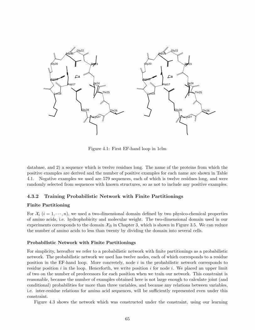
Asp17

Lys18

Asp19

Gly20

Asp21Gly22

Thr23

Ile24

Thr25

Thr26

Lys27

Glu28

Ca

Asp17

Lys18

Asp19

Gly20

Asp21Gly22

Thr23

Ile24

Thr25

Thr26

Lys27

Glu28

Ca

Figure 4.1: First EF-hand loop in 1clm

database, and 2) a sequence which is twelve residues long. The name of the proteins from which thepositive examples are derived and the number of positive examples for each name are shown in Table4.1. Negative examples we used are 579 sequences, each of which is twelve residues long, and wererandomly selected from sequences with known structures, so as not to include any positive examples.

4.3.2 Training Probabilistic Network with Finite Partitionings

Finite Partitioning

For Xi (i = 1, · · · , n), we used a two-dimensional domain defined by two physico-chemical propertiesof amino acids, i.e. hydrophobicity and molecular weight. The two-dimensional domain used in ourexperiments corresponds to the domain XB in Chapter 3, which is shown in Figure 3.5. We can reducethe number of amino acids to less than twenty by dividing the domain into several cells.

Probabilistic Network with Finite Partitionings

For simplicity, hereafter we refer to a probabilistic network with finite partitionings as a probabilisticnetwork. The probabilistic network we used has twelve nodes, each of which corresponds to a residueposition in the EF-hand loop. More concretely, node i in the probabilistic network corresponds toresidue position i in the loop. Henceforth, we write position i for node i. We placed an upper limitof two on the number of predecessors for each position when we train our network. This constraint isreasonable, because the number of examples obtained here is not large enough to calculate joint (andconditional) probabilities for more than three variables, and because any relations between variables,i.e. inter-residue relations for amino acid sequences, will be sufficiently represented even under thisconstraint.

Figure 4.3 shows the network which was constructed under the constraint, using our learning

65

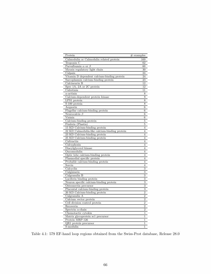
Protein # examples

Calmodulin or Calmodulin related protein 169Troponin C 62Parvalbumin α or β 60Myosin regulatory light chain 30Calpain 24Vitamin D dependent calcium-binding protein 24Sarcoplasmin calcium-binding protein 23Calcineurin B 12Spec 1A, 2A or 2C protein 12Calretinin 11α-actinin 8Calcium-dependent protein kinase 8LPS1 protein 8S-100 protein 8Aequorin 6Flagellar calcium-binding protein 6Neurocalcin β 6Visinin 6Calcium-binding protein 5Fimbrin (Plastin) 515 KD Calcium-binding protein 422 KD Calmodulin-like calcium-binding protein 423 KD Calcium-binding protein 425 KD Calcium-binding protein 4Caltractin 4Calcyphosin 4Diacylglycerol kinase 4Oncomodulin 4Optic lobe calcium-binding protein 4Plasmodial specific protein 4Probable calcium-binding protein 4Sorcin 4Calcyclin 3Calgizzarin 3Calgranulin B 3Luciferin binding protein 3Neuron specific calcium-binding protein 3Osteonectin precursor 3Placental calcium-binding protein 320 KD Calcium-binding protein 2Calgranulin A 2Calcium vector protein 2Cell division control protein 2Recoverin 2Spectrin α-chain 2Chemotactic cytokin 1Matrix glycoprotein sc1 precursor 1Protein MRP-126 1QR1 protein precursor 1S-modulin 1

Table 4.1: 579 EF-hand loop regions obtained from the Swiss-Prot database, Release 28.0

66

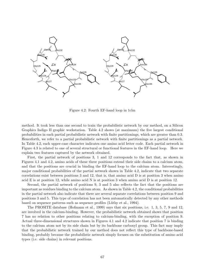
Asp126

Ile127

Asp128

Gly129

Asp130

Gly131 His132

Ile133

Asn134

Tyr135

Glu136

Glu137

Ca

Asp126

Ile127

Asp128

Gly129

Asp130

Gly131 His132

Ile133

Asn134

Tyr135

Glu136

Glu137

Ca

Figure 4.2: Fourth EF-hand loop in 1clm

method. It took less than one second to train the probabilistic network by our method, on a SiliconGraphics Indigo II graphic workstation. Table 4.2 shows (at maximum) the five largest conditionalprobabilities in each partial probabilistic network with finite partitionings, which are greater than 0.3.Henceforth, we refer to a partial probabilistic network with finite partitionings as a partial network.In Table 4.2, each upper-case character indicates one amino acid letter code. Each partial network inFigure 4.3 is related to one of several structural or functional features in the EF-hand loop. Here weexplain two features captured by the network obtained.

First, the partial network of positions 3, 1 and 12 corresponds to the fact that, as shown inFigures 4.1 and 4.2, amino acids of these three positions extend their side chains to a calcium atom,and that the positions are crucial in binding the EF-hand loop to the calcium atom. Interestingly,major conditional probabilities of the partial network shown in Table 4.2, indicate that two separatecorrelations exist between positions 3 and 12, that is, that amino acid D is at position 3 when aminoacid E is at position 12, while amino acid N is at position 3 when amino acid D is at position 12.

Second, the partial network of positions 9, 3 and 5 also reflects the fact that the positions areimportant as residues binding to the calcium atom. As shown in Table 4.2, the conditional probabilitiesin the partial network also indicate that there are several separate correlations between position 9 andpositions 3 and 5. This type of correlation has not been automatically detected by any other methodsbased on sequence patterns such as sequence profiles (Luthy et al., 1994).

The PROSITE database (Hofmann et al., 1999) says that six positions, i.e. 1, 3, 5, 7, 9 and 12,are involved in the calcium-binding. However, the probabilistic network obtained shows that position7 has no relation to other positions relating to calcium-binding, with the exception of position 9.Actual three-dimensional structures shown in Figures 4.1 and 4.2 indicate that position 7 is bindingto the calcium atom not by its side chain but by its backbone carboxyl group. This fact may implythat the probabilistic network trained by our method does not reflect this type of backbone-basedbinding, probably because the probabilistic network simply focuses on the substitution of amino acidtypes (i.e. side chains) in relevant positions.

67

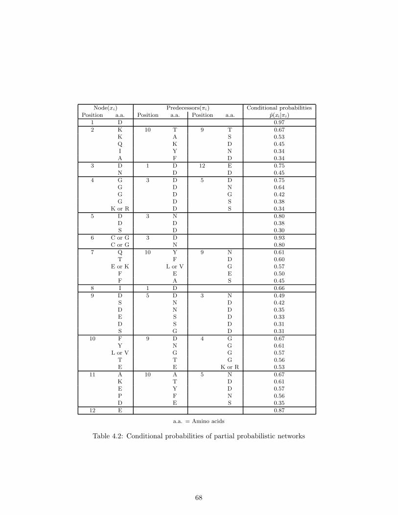
Node(xi) Predecessors(πi) Conditional probabilitiesPosition a.a. Position a.a. Position a.a. p(xi|πi)

1 D 0.97

2 K 10 T 9 T 0.67K A S 0.53Q K D 0.45I Y N 0.34A F D 0.34

3 D 1 D 12 E 0.75N D D 0.45

4 G 3 D 5 D 0.75G D N 0.64G D G 0.42G D S 0.38

K or R D S 0.34

5 D 3 N 0.80D D 0.38S D 0.30

6 C or G 3 D 0.93C or G N 0.80

7 Q 10 Y 9 N 0.61T F D 0.60

E or K L or V G 0.57F E E 0.50F A S 0.45

8 I 1 D 0.66

9 D 5 D 3 N 0.49S N D 0.42D N D 0.35E S D 0.33D S D 0.31S G D 0.31

10 F 9 D 4 G 0.67Y N G 0.61

L or V G G 0.57T T G 0.56E E K or R 0.53

11 A 10 A 5 N 0.67K T D 0.61E Y D 0.57P F N 0.56D E S 0.35

12 E 0.87

a.a. = Amino acids

Table 4.2: Conditional probabilities of partial probabilistic networks

68

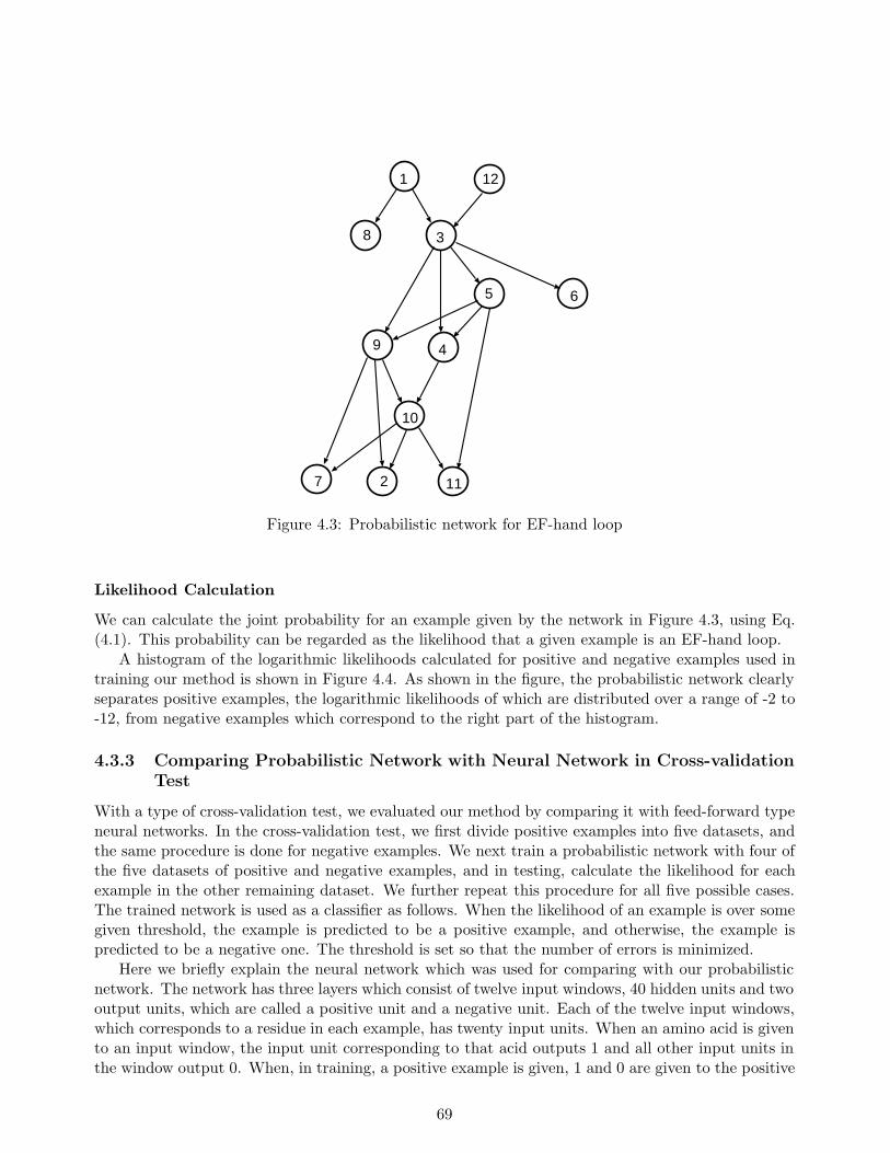
9

1

8

12

3

5 6

4

7 2

10

11

Figure 4.3: Probabilistic network for EF-hand loop

Likelihood Calculation

We can calculate the joint probability for an example given by the network in Figure 4.3, using Eq.(4.1). This probability can be regarded as the likelihood that a given example is an EF-hand loop.

A histogram of the logarithmic likelihoods calculated for positive and negative examples used intraining our method is shown in Figure 4.4. As shown in the figure, the probabilistic network clearlyseparates positive examples, the logarithmic likelihoods of which are distributed over a range of -2 to-12, from negative examples which correspond to the right part of the histogram.

4.3.3 Comparing Probabilistic Network with Neural Network in Cross-validationTest

With a type of cross-validation test, we evaluated our method by comparing it with feed-forward typeneural networks. In the cross-validation test, we first divide positive examples into five datasets, andthe same procedure is done for negative examples. We next train a probabilistic network with four ofthe five datasets of positive and negative examples, and in testing, calculate the likelihood for eachexample in the other remaining dataset. We further repeat this procedure for all five possible cases.The trained network is used as a classifier as follows. When the likelihood of an example is over somegiven threshold, the example is predicted to be a positive example, and otherwise, the example ispredicted to be a negative one. The threshold is set so that the number of errors is minimized.

Here we briefly explain the neural network which was used for comparing with our probabilisticnetwork. The network has three layers which consist of twelve input windows, 40 hidden units and twooutput units, which are called a positive unit and a negative unit. Each of the twelve input windows,which corresponds to a residue in each example, has twenty input units. When an amino acid is givento an input window, the input unit corresponding to that acid outputs 1 and all other input units inthe window output 0. When, in training, a positive example is given, 1 and 0 are given to the positive

69

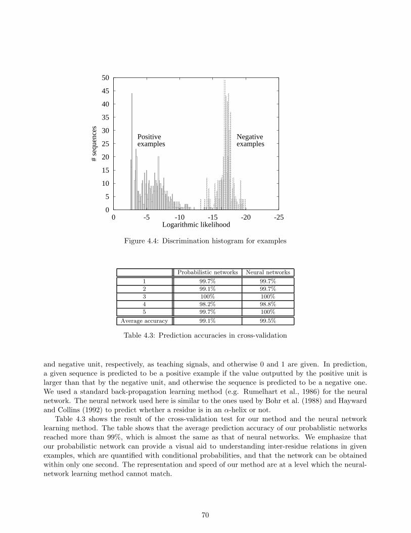
0

5

10

15

20

25

30

35

40

45

50

-25-20-15-10-50

# se

quen

ces

Logarithmic likelihood

Positiveexamples

Negativeexamples

Figure 4.4: Discrimination histogram for examples

Probabilistic networks Neural networks

1 99.7% 99.7%

2 99.1% 99.7%

3 100% 100%

4 98.2% 98.8%

5 99.7% 100%

Average accuracy 99.1% 99.5%

Table 4.3: Prediction accuracies in cross-validation

and negative unit, respectively, as teaching signals, and otherwise 0 and 1 are given. In prediction,a given sequence is predicted to be a positive example if the value outputted by the positive unit islarger than that by the negative unit, and otherwise the sequence is predicted to be a negative one.We used a standard back-propagation learning method (e.g. Rumelhart et al., 1986) for the neuralnetwork. The neural network used here is similar to the ones used by Bohr et al. (1988) and Haywardand Collins (1992) to predict whether a residue is in an α-helix or not.

Table 4.3 shows the result of the cross-validation test for our method and the neural networklearning method. The table shows that the average prediction accuracy of our probablistic networksreached more than 99%, which is almost the same as that of neural networks. We emphasize thatour probabilistic network can provide a visual aid to understanding inter-residue relations in givenexamples, which are quantified with conditional probabilities, and that the network can be obtainedwithin only one second. The representation and speed of our method are at a level which the neural-network learning method cannot match.

70

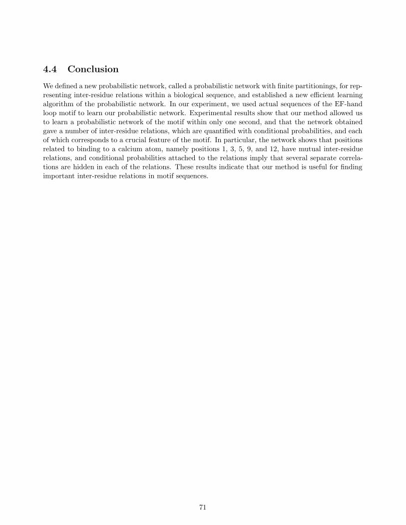
4.4 Conclusion

We defined a new probabilistic network, called a probabilistic network with finite partitionings, for rep-resenting inter-residue relations within a biological sequence, and established a new efficient learningalgorithm of the probabilistic network. In our experiment, we used actual sequences of the EF-handloop motif to learn our probabilistic network. Experimental results show that our method allowed usto learn a probabilistic network of the motif within only one second, and that the network obtainedgave a number of inter-residue relations, which are quantified with conditional probabilities, and eachof which corresponds to a crucial feature of the motif. In particular, the network shows that positionsrelated to binding to a calcium atom, namely positions 1, 3, 5, 9, and 12, have mutual inter-residuerelations, and conditional probabilities attached to the relations imply that several separate correla-tions are hidden in each of the relations. These results indicate that our method is useful for findingimportant inter-residue relations in motif sequences.

71

Chapter 5

Supervised Learning of Hidden MarkovModels

5.1 Introduction

Hidden Markov Models (hereafter referred to as HMMs) have been proven to be a useful tool fora number of subjects in computational molecular biology (Eddy, 1996; Durbin et al., 1998), suchas protein modeling (Stultz, White, & Smith, 1993; White, Smith, & Smith, 1994; Krogh et al.,1994a; Baldi et al., 1994; Baldi & Chauvin, 1994a), gene recognition (Churchill, 1989; Krogh, Mian,& Haussler, 1994b; Krogh, 1997), and secondary structure prediction (Asai, Hayamizu, & Handa,1993). Among these various applications, the most popular application of an HMM in this field hasbeen the construction of an HMM-based profile to represent multiple biological sequences belongingto a single class such as a superfamily. The main theme in generating such a profile is to improve thesensitivity of the model to achieve high accuracy for new sequences in several tasks such as databasesearch or data validation. In the molecular biology field, however, this theme is often subject to astrong constraint, in which the number of available biological sequences belonging to a single classis extremely small, since the sequences can be obtained only through money- and time-consumingbiochemical experiments.

As mentioned in Chapter 2, in training parameters of an HMM, there is a widely used and efficientlearning method, called the Baum-Welch or Forward-Backward (Baum, 1972). The Baum-Welchalgorithm is based on EM (Expectation-Maximization) algorithm (Dempster, Laird, & Rubin, 1977)which trains a given model so that the likelihoods of the training sequences are maximized. However,for the situation in which only a small training dataset is given, it had been pointed out that theBaum-Welch algorithm cannot always provide sufficient discrimination ability (Brown et al., 1993).In contrast to the Baum-Welch’s reestimation rules which let the parameters skip about within theirspace, Baldi et al. (Baldi & Chauvin, 1994b) proposed a smooth learning algorithm which gradientlyoptimizes parameters and can be executed by even on-line learning. This smooth algorithm mightenhance the sensitively of the HMMs trained.

Under these circumstances, we established a new learning method for training an HMM of acertain biological class not only from examples belonging to the class but also from examples whichdo not (Mamitsuka, 1996, 1997). In our method, we first change the probability parameters of a givenHMM into real-valued parameters and prepare an error-distance function which measures an error-distance between the real likelihood and the target likelihood for a given training sequence. To trainthe parameters of an HMM, we then use a gradient descent learning algorithm (Fletcher, 1987) tominimize the energy function prepared. In other words, our method implement new supervised learning

72

of an HMM while the Baum-Welch is based exclusively on unsupervised learning. Furthermore, ourmethod is a smooth algorithm in parameter optimization, with a computation time per iteration inlearning on the same order as that of the Baum-Welch algorithm.

Before we established our new method, several methods had been proposed in the computationalmolecular biology field to improve the sensitivity of an HMM for unknown sequence data. Kroghand Mitchison (1995) and Eddy et al. (1995) independently proposed original learning methods forstochastic models to solve the problem that the probability distribution trained by usual maximumlikelihood criterion is likely to pick out minor data included in training examples. They used onlypositive examples, i.e. the training examples belonging to the class which should be represented by amodel, and using the criterion called maximum discrimination or maximum entropy, they introducedslight modification of Baum-Welch’s re-estimation rules in training an HMM to correct amino acidbiases included in given data. Note that in proposing our method, we wished to consider a new learningmethod itself which is both applicable to any HMM structure and also improves the discriminationaccuracy for unknown sequences so that it out-performs conventional methods such as Baum-Welch.

We summarize the original characteristics of our method as follows:

1) Supervised learning of hidden Markov models.Our learning method allows us to train HMMs with a supervised learning algorithm, namely,to train HMMs using data consisting of a number of discrete or continuous classes or datahaving real-valued labels. However, in the context of natural language processing which is themajor application field of HMMs, most of the learning algorithms proposed to train HMMs arebased on unsupervised learning, and Bahl et al. (1986), which proposed a supervised learningalgorithm for HMMs, has been a unique work. Their method trains HMMs with both positiveand negative examples of a given class, based on the maximum mutual information criterion,but it cannot deal with data consisting of continuous classes or data having real-valued labels.Thus, no supervised learning algorithm able to deal with such data, had ever been proposed intraining HMMs until we established our method, to the best of our knowledge.

2) Fully-connected models tested.In the field of natural language processing and computational molecular biology, in each of whichHMMs have been extensively used, particularly wide usage has been made of a type of HMM,called a left-to-right HMM, in which any arc has to go from a state A to a state B in the rightside of A. On the other hand, in our experiments, we used a fully-connected HMM in which anarc which starts from a state may go to any state. That is, we used a flexible model which isfree of any constraint. In other words, we can say that in our experiment, we attempted to learnnot only the probability parameters of an HMM, but also the structure of the HMM itself.

We performed two experiments. In the first experiment, we used the lipocalin family motif, andgenerated both positive examples, each of which corresponds to a part of a lipocalin sequence, andnegative ones, each of which does not belong to the lipocalin family but has the motif. We evaluatedour method with a type of cross-validation test using fully-connected HMMs with six to fourteenstates, and compared the results obtained with those of the Baum-Welch and Baldi algorithms. Theresults indicate that our method makes fewer discrimination errors than the other two methods. Fromthese results, we conclude that the use of negative examples is effective in learning the parametersof an HMM, and that our method is useful for training an HMM with both positive and negativeexamples.

The second experiment actually consisted of two experiments. In the first, we verified the discrim-ination ability of our supervised learning method compared with that of two other methods, i.e. a

73

back-propagation neural network and the Baum-Welch learning of an HMM. In this experiment, weused actual peptide data in association with their real-valued ability to activate T-cell proliferation,which data was obtained from the MHCPEP database developed by Brusic et al. (1997). The exper-iment was performed by conducting a cross-validation test while varying the proportion of trainingdata to all obtained data. The result of this experiment shows that at any proportion of training datato all data, the average discrimination accuracy of our method was approximately 2 – 15% better thanother methods, i.e. the Baum-Welch reestimation for fully-connected or alignment HMMs and theback-propagation neural network, which had been regarded as the most accurate method in predictingMHC binding peptides. From this result, we conclude that our method was superior in discriminationability to conventional methods in the field of predicting peptides that bind to MHC.

Second, from the MHCPEP database, we obtained peptides which bind to an MHC protein, calledHLA-A2, and trained 100 HMMs using the peptides with our supervised learning algorithm. Out ofthe 100 models trained for HLA-A2, we chose the one which could explain the data best and showedthe HMM. Using the model trained by the data of HLA-A2, we randomly generated peptides whichare expected to have a high ability to bind to HLA-A2, but which are not yet known. From thisexperiment, we ascertained that an HMM trained by our algorithm captures sequence patterns intraining data separately, and found that the extracted patterns include not only existing motifs ofMHC binding peptides but also new sequence patterns, each of which characterizes a part of thetraining peptides.

A brief note on the latest information regarding supervised learning of HMMs: No new method onsupervised learning of an HMM has been proposed since we established our method, but Krogh andRiis proposed a new method for supervised learning of an HMM, called a class HMM (CHMM) (Krogh& Riis, 1999). The CHMM uses a number of techniques which are the same as those used in our methodand it can train an HMM using symbol sequences which are categorized in one or more classes (labels);however the CHMM has a disadvantage in that it cannot deal with continuous classes. In contrast,our learning algorithm train an HMM using sequences with not only continuous classes but also real-valued labels. From this viewpoint, we can say that even now, our method has a significant advantagein the field of training algorithms of HMMs.

5.2 Hidden Markov Models

We recall the definition of hidden Markov model (HMM), forward and backward probabilities, and ξand γ, which are given in Chapter 2.

Definition 5.1 (Hidden Markov Model) A hidden Markov model H is a 7-tuple 〈Σ, Q, I, F,E,A,B〉,where:(i) Σ is a finite alphabet.(ii) Q is a finite set of states.(iii) I ⊆ Q is a finite set of initial states.(iv) F ⊆ Q is a finite set of final states.(v) E ⊆ Q × Q is a finite set of arcs. An arc (i, j) ∈ E is also denoted by eij .(vi) A = (aij)i,j∈Q is a matrix of state transition probabilities, i.e. aij is the probability that is attachedto arc eij which indicates the transition from state i to j, where

∑

j∈Q aij = 1 is assumed for eachi ∈ Q.(vii) B = (bj(c))j∈Q,c∈Σ is a matrix of symbol output probabilities, i.e. bj(c) is the probability that isattached to state j which indicates that state j outputs symbol c, where

∑

c∈Σ bj(c) = 1 is assumedfor each j ∈ Q. 2

74

Definition 5.2 (Forward Probability) (Rabiner, 1989) Let H = 〈Σ, Q, I, F,E,A,B〉 be an HMM.For convenience, let Q = {1, · · · ,M}, Σ = {1, · · · , L}. For a symbol sequence σ = σ1 · · · σnσ , 1 ≤ t ≤nσ and a state j, the forward probability ασ[t, j] is the probability that the partial sequence σ1 · · · σt

is generated, and that the state at time t is j. For t = 0 and a state j, the forward probability ασ[0, j]is the probability that no symbol is generated, and that the state at time 0 is j. 2

Definition 5.3 (Backward Probability) (Rabiner, 1989) Let H = 〈Σ, Q, I, F,E,A,B〉 be an HMM.For convenience, let Q = {1, · · · ,M}, Σ = {1, · · · , L}. For a symbol sequence σ = σ1 · · · σnσ ,0 ≤ t ≤ nσ − 1 and a state i, the backward probability βσ[t, i] is the probability that the partialsequence σt+1 · · · σnσ is generated, and that the state at time t is i. For t = nσ and a state i, thebackward probability βσ[nσ, i] is the probability that no symbol is generated, and that the state attime nσ is i. 2

Note that∑

1≤i≤M ασ[nσ + 1, i]βσ [nσ + 1, i], as well as∑

1≤i≤M ασ[0, i]βσ [0, i], corresponds to thelikelihood that the given training sequence σ is generated by the HMM H, i.e. P (σ|H).

Our learning algorithm, as well as the Baum-Welch algorithm, uses the following two probabilitiesξ and γ.

Definition 5.4 (ξ and γ) (Rabiner, 1989) Let H = 〈Σ, Q, I, F,E,A,B〉 be an HMM. For conve-nience, let Q = {1, · · · ,M}, Σ = {1, · · · , L}. For a symbol sequence σ = σ1 · · · σnσ , 0 ≤ t ≤ nσ − 1and two states i and j, ξσ[t, i, j] is the probability that the σ is generated by the H, and that the twostates at times t and t + 1 are i and j, respectively. Similarly, for a symbol sequence σ = σ1 · · · σnσ ,0 ≤ t ≤ nσ and a state i, γσ[t, i] is the probability that the σ is generated by the H, and that thestate at time t is i. 2

The probabilities ξ and γ are calculated using the forward and backward probabilities as follows:

ξσ[t, i, j] =ασ[t, i]aijbj(σt+1)βσ[t + 1, j]

P (σ|H)(0 ≤ t ≤ nσ − 1), (5.1)

γσ[t, i] =ασ[t, i]βσ [t, i]

P (σ|H)(0 ≤ t ≤ nσ). (5.2)

Proposition 5.5 (Time Complexity of Forward, Backward, ξ and γ)The time complexity of the forward and backward algorithms for an HMM is O(N · M2), where N

is the length of a given sequence and M is the number of states in the HMM. The time complexity ofcalculating ξ and γ is also O(N · M2).(Proof)The time complexity of the forward and backward algorithm depends on the calculation of step 2 inAlgorithm 2.5 and step 3 in Algorithm 2.15. The time complexity of calculating γ and ξ also dependson them. 2

5.3 Supervised Learning Algorithm for Hidden Markov Models

We introduce real-valued parameters wij and vj(c), which are used in (Bridle, 1990) and (Baldi &Chauvin, 1994b), as follows:

aij =eλ1wij

∑

k eλ1wik, bj(c) =

eλ2vj(c)

∑

k eλ2vj(k), (5.3)

(∑

1≤j≤M

aij = 1, aij ≥ 0,∑

1≤c≤L

bj(c) = 1, bj(c) ≥ 0.)

75

where λ1 and λ2 are constants. The equations allow wij and vj(c) to be any real-value, satisfying theconstraints of aij and bj(c) given by Definition 5.1.

We define an error-distance function.

Definition 5.6 (Error-distance Function) (Mamitsuka, 1996) Let H = 〈Σ, Q, I, F,E,A,B〉 be anHMM. Let Ξ be a set of symbol sequences. Let pσ ∈ [0, 1] be the likelihood that a sequence σ ∈ Ξis generated by an H, i.e. P (σ|H), and we call pσ the real likelihood. Let p∗σ ∈ [0, 1] be a real-valuewhich we call the target likelihood. For a sequence σ, let Dσ be a positive real-value given by thefollowing form:

Dσ = (log(p∗σpσ

))2.

For a sequence σ, let gσ ∈ [0, 1] be a real-value given as follows:

gσ =Dmax − Dσ

Dmax,

where Dmax is a fixed positive real-value, which is larger than Dσ|σ∈Ξ.For a set of sequences Ξ, we define an error-distance function F (Ξ) ∈ [0,∞] as follows:

F (Ξ) =∑

σ∈Ξ

− log gσ. (5.4)

2

For each sequence σ, the purpose of our learning algorithm is that Dσ → 0 . Here, for each σ,gσ → 1 if Dσ → 0. Furthermore, gσ → 1 for each σ means that F (Ξ) → 0. Thus, in order to attainthe purpose of our learning algorithm, we have to minimize the F (Ξ). In minimizing the F (Ξ), weobtain a smooth learning algorithm for optimizing real-valued parameters, wij and vj(c), as follows:

Algorithm 5.7 (Supervised Learning for Hidden Markov Models) (Mamitsuka, 1996)input: a set of symbol sequences Ξ and initial aij and bj(c)output: trained aij and bj(c)1: Calculate wij and vj(c) from the initial aij and bj(c), using (5.4).2: Repeat the following two steps until a stopping condition is satisfied, usually until the changes inthe aij and bj(c) become smaller than a certain preset amount.2-1: Update the wij and vj(c) using (5.5) and (5.6).2-2: Calculate aij and bj(c) from wij and vj(c), using (5.4).

wnewij = wold

ij + Ca∂F (Ξ)

∂wij

= woldij + Ca

∑

σ∈Ξ

dσ

(Dmax − Dσ)

∑

0≤t≤nσ−1

(ξσ[t, i, j] − aijγσ[t, i]), (5.5)

vj(c)new = vj(c)

old + Cb

∂F (Ξ)

∂vj(c)

= vj(c)old + Cb

∑

σ∈Ξ

dσ

(Dmax − Dσ)

∑

1≤t≤nσ

(γσ [t|σt = c, j] − bj(c)γσ [t, j]), (5.6)

where dσ = log(p∗σpσ

) and Ca and Cb are positive constants. 2

76

We here give two propositions relevant to the partial derivatives of aij .

Proposition 5.8

∂pσ

∂aik

=∑

0≤t≤nσ−1

ασ[t, i]bk(σt+1)βσ [t + 1, k]

2

Proposition 5.9

∂aij

∂wik

= λaij(δjk − aik) , δjk =

{

1 if j = k,0 otherwise.

2

Then, using the two propositions, we show the derivation of ∂F (Ξ)∂wij

in (5.5).

∂F (Ξ)

∂wij=

∑

k

∑

s

∂ log gσ

∂aik

∂aik

∂wij

=∑

σ∈Ξ

2dσ

pσ(d2max − d2

σ)

∑

k

∂pσ

∂aik

∂aik

∂wij

= λ∑

σ∈Ξ

2dσ

pσ(d2max − d2

σ)

∑

k

(δkj − aij)∑

0≤t≤nσ−1

ασ[t, i]aikbk(σt+1)βσ [t + 1, k]

since Propositions 5.8 and 5.9

= λ∑

σ∈Ξ

2dσ

(d2max − d2

σ)

∑

k

(δkj − aij)∑

0≤t≤nσ−1

ξσ[t, i, k]

= Consta∑

σ∈Ξ

dσ

(d2max − d2

σ)

∑

0≤t≤nσ−1

(ξσ[t, i, j] − aijγσ[t, i]),

where Consta is a constant.We can derive (5.6) in a similar manner. In (5.5) and (5.6), if a part, dσ

(Dmax−Dσ) , is removed, both

equations are equal to those of Baldi’s smooth algorithm. Furthermore, from (5.5) and (5.6), we canderive an on-line supervised learning algorithm as done in Baldi and Chauvin (1994b).

Algorithm 5.10 (On-line Supervised Learning for Hidden Markov Models) (Mamitsuka, 1996)input: a set of symbol sequences Ξ and initial aij and bj(c)output: trained aij and bj(c)1: Calculate wij and vj(c) from the initial aij and bj(c), using (5.4).2: For each sequence σ, repeat the following two steps until a stopping condition is satisfied.2-1: Update the wij and vj(c) using (5.7) and (5.8).2-2: Calculate aij and bj(c) from wij and vj(c), using (5.4).

wnewij = wold

ij + C ′a

dσ

(Dmax − Dσ)

∑

0≤t≤nσ−1

(ξσ[t, i, j] − aijγσ[t, i]), (5.7)

vj(c)new = vj(c)

old + C ′b

dσ

(Dmax − Dσ)

∑

1≤t≤nσ

(γσ[t|σt = c, j] − bj(c)γσ [t, j]), (5.8)

where dσ = log(p∗σpσ

) and C ′a and C ′

b are positive constants. 2

77

Proposition 5.11 (Time Complexity of Our Learning Algorithm)The time complexity of one iteration of our learning algorithm given by Algorithm 5.10 is O(N ·M2),while that given by Algorithm 5.7 is O(N · M2 · W ), where W is the number of symbol sequences, Nis the length of a given sequence and M is the number of states in an HMM.(Proof)The time complexity of Algorithm 5.10 depends on calculating γ and ξ for a given sequence, and thetime complexity of them is given by O(N · M2) in Proposition 5.5. On the other hand, in Algorithm5.7, calculating the γ and ξ has to be done for all symbol sequences at once, and then the complexityof the algorithm is given by O(N · M2 · W ). 2

5.4 Experimental Results – 1

In this experiment, we evaluated our method (hereafter referred to as MA) by applying it to a sequenceclassification problem, and compared the results with those of the Baum-Welch (hereafter referred toas BW) and the Baldi algorithm (hereafter referred to as BA). We used here a fully-connected HMM,which has only one initial state and one final state, neither of which output any symbols. That is, theinitial state has arcs going to any state except for the final state, and any state except for the finalstate has arcs going to any state other than the initial state.

Here, let us describe how we set p∗σ in our experiments. Using Algorithm 2.5, we first estimate thelikelihood that a symbol sequence of length n is generated by the fully-connected HMM with uniformdistributions to be approximately 1

M( 1

L)n, which is obtained by assuming aij = 1

Mand bj(c) = 1

L,

where M denotes the number of states, and L denotes the number of symbols. Then, we let p∗σ

be ( 120)0.01×n and ( 1

20)1.99×n for positive and negative examples, respectively, to satisfy the abovecondition.

5.4.1 Data – Lipocalin Family Motif

We used the lipocalin family motif (Peitsch & Boguski, 1991) noted in Release 12.0 of the PROSITEdatabase (Bairoch, P.Bucher, & Hofmann, 1996). The motif is ‘[DENG] - X - [DENQGSTARK]- X(0,2) - [DENQARK] - [LIVFY] - {CP} - G - {C} - W - [FYWLRH] - X - [LIVMTA]’, whereno amino acids from among those enclosed in { } are not permitted, but either zero, one or twoamino acids are permitted at the X(0,2). Thus, any sequence having the motif is twelve to four-teen residues long. Figure 5.1 shows a three-dimensional structure (Peitsch & Boguski, 1990) of thesequence having the motif in human apolipoprotein which belongs to the lipocalin family, and thestructure is constructed from the coordinates noted in the PDB database (Bernstein et al., 1977) as‘2apd’. The structure shown in the figure corresponds to a part of a β-strand, and the amino acidsequence is DVNKYLGRWYEI from right to left in the figure. From the Swiss-Prot database Release29.0 (Bairoch & Apweiler, 1996), we obtained 142 sequences, each of which contains the motif. Of thesequences, we used 99 sequences as positive examples which were included in actual lipocalin familyprotein sequences, and 43 sequences as negative examples which had the motif but were not in anylipocalin family proteins.

The goal of the problem which we now deal with is to distinguish positive examples from negativeones. Note that the problem is rather difficult in that we have to separate positive examples fromfalse positive examples, since the negative examples as well as positive ones have the motif and wecannot recognize positive examples from all the sequences using the motif only.

78

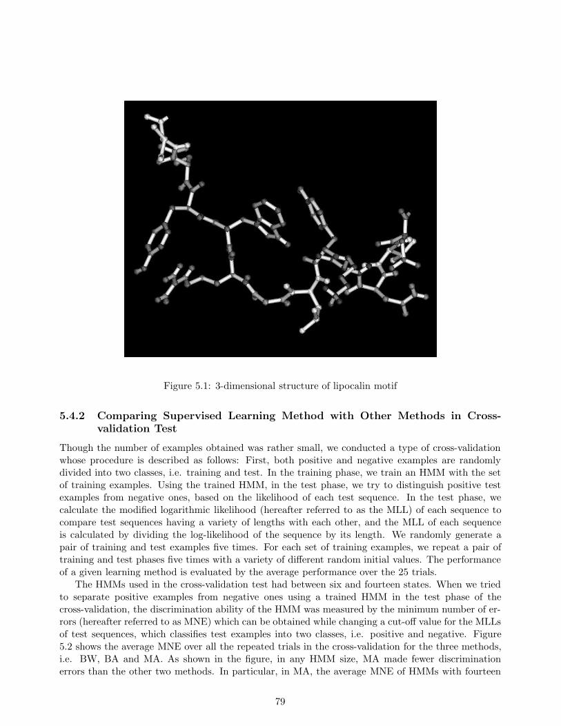
Figure 5.1: 3-dimensional structure of lipocalin motif

5.4.2 Comparing Supervised Learning Method with Other Methods in Cross-validation Test

Though the number of examples obtained was rather small, we conducted a type of cross-validationwhose procedure is described as follows: First, both positive and negative examples are randomlydivided into two classes, i.e. training and test. In the training phase, we train an HMM with the setof training examples. Using the trained HMM, in the test phase, we try to distinguish positive testexamples from negative ones, based on the likelihood of each test sequence. In the test phase, wecalculate the modified logarithmic likelihood (hereafter referred to as the MLL) of each sequence tocompare test sequences having a variety of lengths with each other, and the MLL of each sequenceis calculated by dividing the log-likelihood of the sequence by its length. We randomly generate apair of training and test examples five times. For each set of training examples, we repeat a pair oftraining and test phases five times with a variety of different random initial values. The performanceof a given learning method is evaluated by the average performance over the 25 trials.

The HMMs used in the cross-validation test had between six and fourteen states. When we triedto separate positive examples from negative ones using a trained HMM in the test phase of thecross-validation, the discrimination ability of the HMM was measured by the minimum number of er-rors (hereafter referred to as MNE) which can be obtained while changing a cut-off value for the MLLsof test sequences, which classifies test examples into two classes, i.e. positive and negative. Figure5.2 shows the average MNE over all the repeated trials in the cross-validation for the three methods,i.e. BW, BA and MA. As shown in the figure, in any HMM size, MA made fewer discriminationerrors than the other two methods. In particular, in MA, the average MNE of HMMs with fourteen

79

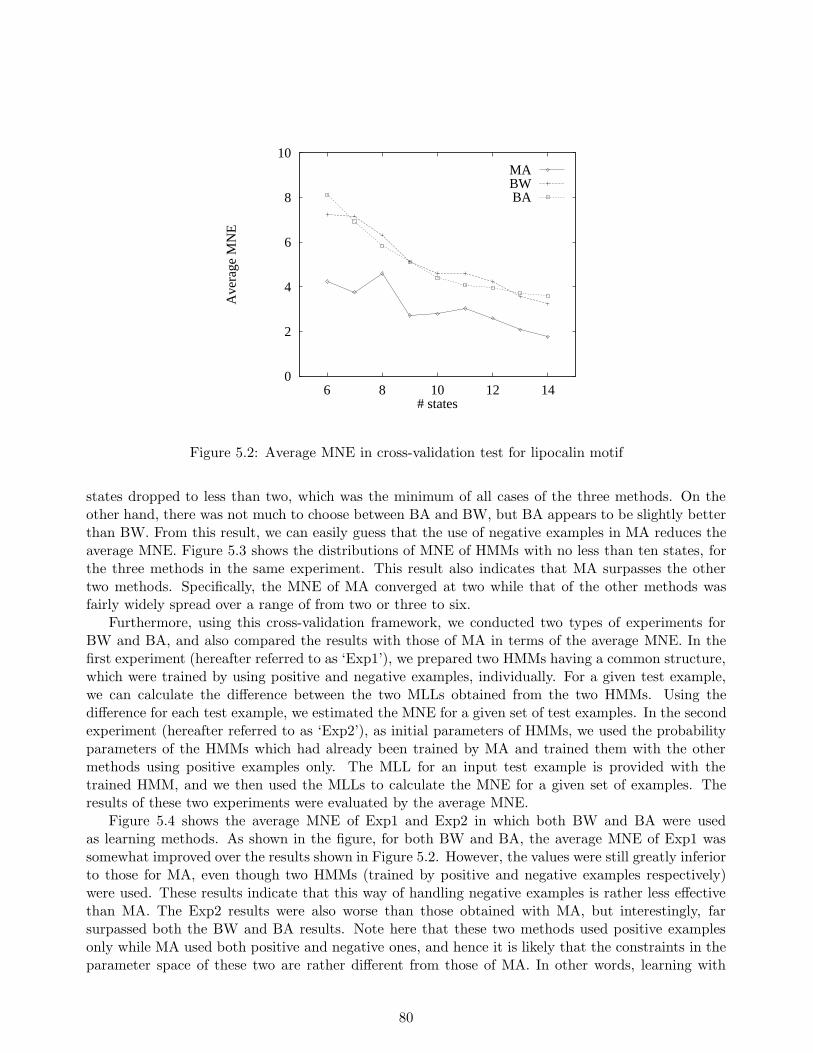
0

2

4

6

8

10

6 8 10 12 14

Ave

rage

MN

E

# states

MABWBA

Figure 5.2: Average MNE in cross-validation test for lipocalin motif

states dropped to less than two, which was the minimum of all cases of the three methods. On theother hand, there was not much to choose between BA and BW, but BA appears to be slightly betterthan BW. From this result, we can easily guess that the use of negative examples in MA reduces theaverage MNE. Figure 5.3 shows the distributions of MNE of HMMs with no less than ten states, forthe three methods in the same experiment. This result also indicates that MA surpasses the othertwo methods. Specifically, the MNE of MA converged at two while that of the other methods wasfairly widely spread over a range of from two or three to six.

Furthermore, using this cross-validation framework, we conducted two types of experiments forBW and BA, and also compared the results with those of MA in terms of the average MNE. In thefirst experiment (hereafter referred to as ‘Exp1’), we prepared two HMMs having a common structure,which were trained by using positive and negative examples, individually. For a given test example,we can calculate the difference between the two MLLs obtained from the two HMMs. Using thedifference for each test example, we estimated the MNE for a given set of test examples. In the secondexperiment (hereafter referred to as ‘Exp2’), as initial parameters of HMMs, we used the probabilityparameters of the HMMs which had already been trained by MA and trained them with the othermethods using positive examples only. The MLL for an input test example is provided with thetrained HMM, and we then used the MLLs to calculate the MNE for a given set of examples. Theresults of these two experiments were evaluated by the average MNE.

Figure 5.4 shows the average MNE of Exp1 and Exp2 in which both BW and BA were usedas learning methods. As shown in the figure, for both BW and BA, the average MNE of Exp1 wassomewhat improved over the results shown in Figure 5.2. However, the values were still greatly inferiorto those for MA, even though two HMMs (trained by positive and negative examples respectively)were used. These results indicate that this way of handling negative examples is rather less effectivethan MA. The Exp2 results were also worse than those obtained with MA, but interestingly, farsurpassed both the BW and BA results. Note here that these two methods used positive examplesonly while MA used both positive and negative ones, and hence it is likely that the constraints in theparameter space of these two are rather different from those of MA. In other words, learning with

80

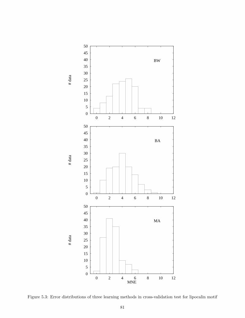
0

5

10

15

20

25

30

35

40

45

50

0 2 4 6 8 10 12

# da

ta

BW

0

5

10

15

20

25

30

35

40

45

50

0 2 4 6 8 10 12

# da

ta

BA

0

5

10

15

20

25

30

35

40

45

50

0 2 4 6 8 10 12

# da

ta

MNE

MA

Figure 5.3: Error distributions of three learning methods in cross-validation test for lipocalin motif

81

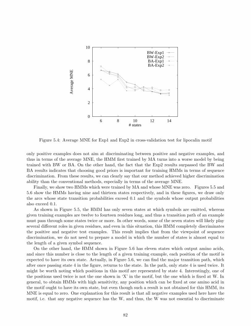
0

2

4

6

8

10

6 8 10 12 14

Ave

rage

MN

E

# states

BW-Exp1BW-Exp2BA-Exp1BA-Exp2

Figure 5.4: Average MNE for Exp1 and Exp2 in cross-validation test for lipocalin motif

only positive examples does not aim at discriminating between positive and negative examples, andthus in terms of the average MNE, the HMM first trained by MA turns into a worse model by beingtrained with BW or BA. On the other hand, the fact that the Exp2 results surpassed the BW andBA results indicates that choosing good priors is important for training HMMs in terms of sequencediscrimination. From these results, we can clearly say that our method achieved higher discriminationability than the conventional methods, especially in terms of the average MNE.

Finally, we show two HMMs which were trained by MA and whose MNE was zero. Figures 5.5 and5.6 show the HMMs having nine and thirteen states respectively, and in these figures, we draw onlythe arcs whose state transition probabilities exceed 0.1 and the symbols whose output probabilitiesalso exceed 0.1.

As shown in Figure 5.5, the HMM has only seven states at which symbols are emitted, whereasgiven training examples are twelve to fourteen residues long, and thus a transition path of an examplemust pass through some states twice or more. In other words, some of the seven states will likely playseveral different roles in given residues, and even in this situation, this HMM completely discriminatesthe positive and negative test examples. This result implies that from the viewpoint of sequencediscrimination, we do not need to prepare a model in which the number of states is almost equal tothe length of a given symbol sequence.

On the other hand, the HMM shown in Figure 5.6 has eleven states which output amino acids,and since this number is close to the length of a given training example, each position of the motif isexpected to have its own state. Actually, in Figure 5.6, we can find the major transition path, whichafter once passing state 4 in the figure, returns to the state. In the path, only state 4 is used twice. Itmight be worth noting which positions in this motif are represented by state 4. Interestingly, one ofthe positions used twice is not the one shown in ‘X’ in the motif, but the one which is fixed at W. Ingeneral, to obtain HMMs with high sensitivity, any position which can be fixed at one amino acid inthe motif ought to have its own state, but even though such a result is not obtained for this HMM, itsMNE is equal to zero. One explanation for this result is that all negative examples used here have themotif, i.e. that any negative sequence has the W, and thus, the W was not essential to discriminate

82

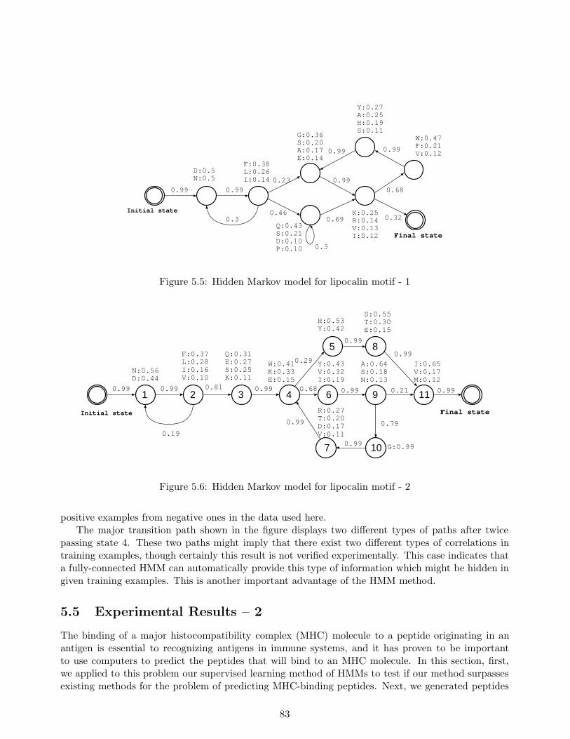
Initial state

F:0.38L:0.26I:0.14

G:0.36S:0.20A:0.17E:0.14

Y:0.27A:0.25H:0.19S:0.11

W:0.47F:0.21V:0.12

K:0.25R:0.14V:0.13I:0.12

Q:0.43S:0.21D:0.10P:0.10

0.99 0.99

0.3

0.23

0.46

0.3

0.69

0.99

0.99 0.99

0.68

0.32

Final state

D:0.5N:0.5

Figure 5.5: Hidden Markov model for lipocalin motif - 1

Initial state

0.99 0.99

0.99

0.99

0.99

0.68

Final state

0.81 0.99

0.79

0.21

0.99

0.290.99

0.99

0.19

N:0.56D:0.44

F:0.37L:0.28I:0.16V:0.10

Q:0.31E:0.27S:0.25K:0.11

W:0.41K:0.33E:0.15

H:0.53Y:0.42

Y:0.43V:0.32I:0.19

S:0.55T:0.30E:0.15

A:0.64S:0.18N:0.13

G:0.99

R:0.27T:0.20D:0.17V:0.11

I:0.65V:0.17M:0.12

1 2 3 4

5

6

7

8

9

10

11

Figure 5.6: Hidden Markov model for lipocalin motif - 2

positive examples from negative ones in the data used here.The major transition path shown in the figure displays two different types of paths after twice

passing state 4. These two paths might imply that there exist two different types of correlations intraining examples, though certainly this result is not verified experimentally. This case indicates thata fully-connected HMM can automatically provide this type of information which might be hidden ingiven training examples. This is another important advantage of the HMM method.

5.5 Experimental Results – 2

The binding of a major histocompatibility complex (MHC) molecule to a peptide originating in anantigen is essential to recognizing antigens in immune systems, and it has proven to be importantto use computers to predict the peptides that will bind to an MHC molecule. In this section, first,we applied to this problem our supervised learning method of HMMs to test if our method surpassesexisting methods for the problem of predicting MHC-binding peptides. Next, we generated peptides

83

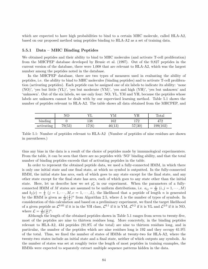
which are expected to have high probabilities to bind to a certain MHC molecule, called HLA-A2,based on our proposed method using peptides binding to HLA-A2 as a set of training data.

5.5.1 Data – MHC Binding Peptides

We obtained peptides and their ability to bind to MHC molecules (and activate T-cell proliferation)from the MHCPEP database developed by Brusic et al. (1997). Out of the 9,827 peptides in thecurrent version of the database, there were 1,008 that are relevant to HLA-A2, which was the largestnumber among the peptides noted in the database.

In the MHCPEP database, there are two types of measures used in evaluating the ability ofpeptides, i.e. the ability to bind to MHC molecules (binding peptides) and to activate T-cell prolifera-tion (activating peptides). Each peptide can be assigned one of six labels to indicate its ability: ‘none(NO)’, ‘yes but little (YL)’, ‘yes but moderate (YM)’, ‘yes and high (YH)’, ‘yes but unknown’ and‘unknown’. Out of the six labels, we use only four: NO, YL, YM and YH, because the peptides whoselabels are unknown cannot be dealt with by our supervised learning method. Table 5.1 shows thenumber of peptides relevant to HLA-A2. The table shows all data obtained from the MHCPEP, and

NO YL YM YH Total

binding 0 138 162 172 472

activating 79(53) 17(6) 46(13) 57(30) 199(102)

Table 5.1: Number of peptides relevant to HLA-A2 (Number of peptides of nine residues are shownin parentheses.)

thus any bias in the data is a result of the choice of peptides made by immunological experimenters.From the table, it can be seen that there are no peptides with ‘NO’ binding ability, and that the totalnumber of binding peptides exceeds that of activating peptides in the table.

In order to represent the obtained peptide data, we used a fully-connected HMM, in which thereis only one initial state and one final state, at which no symbol is outputted. In the fully-connectedHMM, the initial state has arcs, each of which goes to any state except for the final state, and anyother state except for the final state has arcs, each of which goes to any state other than the initialstate. Here, let us describe how we set p∗σ in our experiment. When the parameters of a fully-connected HMM of M states are assumed to be uniform distributions, i.e. aij = 1

M(i, j = 1, · · · ,M)

and bj(c) = 1L

(j = 1, · · · ,M, c = 1, · · · , L), the likelihood that a peptide of length n is generatedby the HMM is given as 1

M( 1

L)n from Algorithm 2.5, where L is the number of types of symbols. In

consideration of this calculation and based on a preliminary experiment, we fixed the target likelihoodof a given peptide as L0.05 if it is in the YH class, L0.1 if it is YM, L0.2 if it is YL and L2.0 if it is NO,where L = 1

M( 1

L)n.

Although the length of the obtained peptides shown in Table 5.1 ranges from seven to twenty-five,most of the peptides are nine to thirteen residues long. More concretely, in the binding peptidesrelevant to HLA-A2, 434 peptides (91.9% of the total) are nine to thirteen residues long, and inparticular, the number of the peptides which are nine residues long is 192 and they occupy 61.9%of the total. Thus, we fixed the number of states of HMMs at twenty-two for HLA-A2, where thetwenty-two states include an initial state and a final state, neither of which outputs any symbols. Asthe number of states was set at roughly twice the length of most peptides in training examples, theHMMs were expected to separately extract multiple sequence patterns hidden in the data.

84

5.5.2 Comparing Supervised Learning Method with Other Methods in Cross-validation Test

We compared the performance of our supervised learning algorithm of an HMM with those of twoother methods. The first of the two was a back-propagation neural network, which had been used inpredicting MHC binding peptides and regarded as the most effective approach. The second was theBaum-Welch algorithm, i.e. the most popular learning algorithm of an HMM. Using the Baum-Welch,we tested two-types of HMMs, i.e. fully-connected and alignment HMMs. A fully-connected HMM isone in which any pair of states is connected, except for the pair of the initial and final states. However,an alignment HMM has been used for aligning multiple sequences and (see Figure 2.14).

Data

In this experiment, testing was done by binary prediction, i.e. YES or NO. Thus, we used activatingpeptides relevant to HLA-A2, because there is no non-binding data in HLA-A2. Table 5.1 shows thenumber of peptides used in this experiment. Note that basically, there is no non-binding peptide in theMHCPEP database, because it gathers peptides that bind to MHC proteins. Thus, in the database,even the peptides which cannot activate T-cell proliferation will bind to MHC proteins. In otherwords, such peptides can be regarded as false-positive examples if a peptide which can activate T-cellproliferation is called a positive example. In this sense, the discrimination experiment performed herewas a severe test. As back-propagation neural networks were used in the comparisons, all peptidesused here were of nine residues, since all previous work based on back-propagation neural networksused only such peptides.

Note that the three methods differ in data usage. Our method used four labels, i.e. YH, YM, YLand NO. On the other hand, back-propagation neural networks were trained by two labels, i.e. YESor NO, as done in Gulukota et al. (1997), and the Baum-Welch algorithm used only YES (YH, YM,YL) since it is an unsupervised learning algorithm.

Back-propagation neural network

We here briefly explain the network used in our experiment, which is the same as the one used byGulukota et al. (1997).

The network has three layers, i.e. an input, a hidden and an output layer, each of which consistsof a fixed number of nodes. The number of input, hidden and output nodes is 180(= 20 × 9), 50 and1, respectively. A set of 20 nodes in the input layer, each of which corresponds to one of 20 types ofamino acids, corresponds to one of nine residues in a given peptide. When a peptide is given, onlyone node in the set of 20 nodes outputs 1 and the other 19 nodes in the set output 0. Any two nodesbetween input and hidden layers and between hidden and output layers are connected by a directededge, to which a weight is attached.

Let xj be the output value of node j and wij be the weight attached to the edge connecting fromnode i to node j. We calculate the xj in the hidden and output layers as follows:

xj = f(∑

i

wijxi), (5.9)

where the function f is a sigmoid function satisfying f(x) = 11+e−x . Weights wij are trained by a

standard back-propagation learning algorithm (Rumelhart et al., 1986). In this learning, 1 is givenas a teaching signal for the output value of this network if a given training peptide is labeled ’YES’;

85

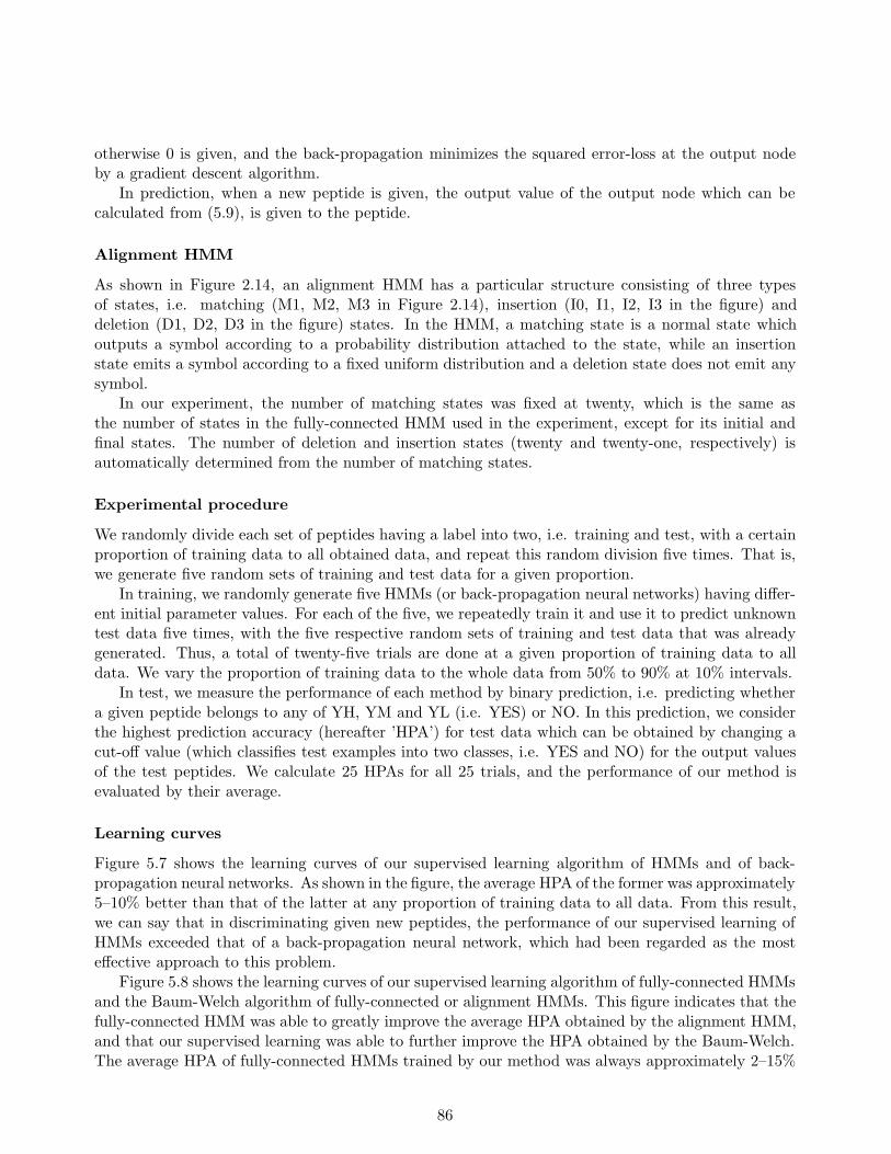
otherwise 0 is given, and the back-propagation minimizes the squared error-loss at the output nodeby a gradient descent algorithm.

In prediction, when a new peptide is given, the output value of the output node which can becalculated from (5.9), is given to the peptide.

Alignment HMM

As shown in Figure 2.14, an alignment HMM has a particular structure consisting of three typesof states, i.e. matching (M1, M2, M3 in Figure 2.14), insertion (I0, I1, I2, I3 in the figure) anddeletion (D1, D2, D3 in the figure) states. In the HMM, a matching state is a normal state whichoutputs a symbol according to a probability distribution attached to the state, while an insertionstate emits a symbol according to a fixed uniform distribution and a deletion state does not emit anysymbol.

In our experiment, the number of matching states was fixed at twenty, which is the same asthe number of states in the fully-connected HMM used in the experiment, except for its initial andfinal states. The number of deletion and insertion states (twenty and twenty-one, respectively) isautomatically determined from the number of matching states.

Experimental procedure

We randomly divide each set of peptides having a label into two, i.e. training and test, with a certainproportion of training data to all obtained data, and repeat this random division five times. That is,we generate five random sets of training and test data for a given proportion.

In training, we randomly generate five HMMs (or back-propagation neural networks) having differ-ent initial parameter values. For each of the five, we repeatedly train it and use it to predict unknowntest data five times, with the five respective random sets of training and test data that was alreadygenerated. Thus, a total of twenty-five trials are done at a given proportion of training data to alldata. We vary the proportion of training data to the whole data from 50% to 90% at 10% intervals.

In test, we measure the performance of each method by binary prediction, i.e. predicting whethera given peptide belongs to any of YH, YM and YL (i.e. YES) or NO. In this prediction, we considerthe highest prediction accuracy (hereafter ’HPA’) for test data which can be obtained by changing acut-off value (which classifies test examples into two classes, i.e. YES and NO) for the output valuesof the test peptides. We calculate 25 HPAs for all 25 trials, and the performance of our method isevaluated by their average.

Learning curves

Figure 5.7 shows the learning curves of our supervised learning algorithm of HMMs and of back-propagation neural networks. As shown in the figure, the average HPA of the former was approximately5–10% better than that of the latter at any proportion of training data to all data. From this result,we can say that in discriminating given new peptides, the performance of our supervised learning ofHMMs exceeded that of a back-propagation neural network, which had been regarded as the mosteffective approach to this problem.

Figure 5.8 shows the learning curves of our supervised learning algorithm of fully-connected HMMsand the Baum-Welch algorithm of fully-connected or alignment HMMs. This figure indicates that thefully-connected HMM was able to greatly improve the average HPA obtained by the alignment HMM,and that our supervised learning was able to further improve the HPA obtained by the Baum-Welch.The average HPA of fully-connected HMMs trained by our method was always approximately 2–15%

86

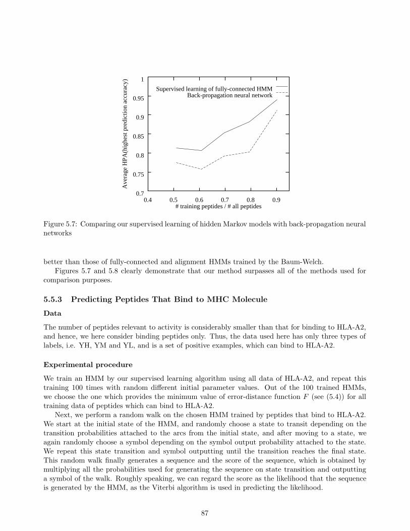
0.7

0.75

0.8

0.85

0.9

0.95

1

0.4 0.5 0.6 0.7 0.8 0.9

Ave

rage

HPA

(hig

hest

pre

dict

ion

accu

racy

)

# training peptides / # all peptides

Supervised learning of fully-connected HMMBack-propagation neural network

Figure 5.7: Comparing our supervised learning of hidden Markov models with back-propagation neuralnetworks

better than those of fully-connected and alignment HMMs trained by the Baum-Welch.Figures 5.7 and 5.8 clearly demonstrate that our method surpasses all of the methods used for

comparison purposes.

5.5.3 Predicting Peptides That Bind to MHC Molecule

Data

The number of peptides relevant to activity is considerably smaller than that for binding to HLA-A2,and hence, we here consider binding peptides only. Thus, the data used here has only three types oflabels, i.e. YH, YM and YL, and is a set of positive examples, which can bind to HLA-A2.

Experimental procedure

We train an HMM by our supervised learning algorithm using all data of HLA-A2, and repeat thistraining 100 times with random different initial parameter values. Out of the 100 trained HMMs,we choose the one which provides the minimum value of error-distance function F (see (5.4)) for alltraining data of peptides which can bind to HLA-A2.

Next, we perform a random walk on the chosen HMM trained by peptides that bind to HLA-A2.We start at the initial state of the HMM, and randomly choose a state to transit depending on thetransition probabilities attached to the arcs from the initial state, and after moving to a state, weagain randomly choose a symbol depending on the symbol output probability attached to the state.We repeat this state transition and symbol outputting until the transition reaches the final state.This random walk finally generates a sequence and the score of the sequence, which is obtained bymultiplying all the probabilities used for generating the sequence on state transition and outputtinga symbol of the walk. Roughly speaking, we can regard the score as the likelihood that the sequenceis generated by the HMM, as the Viterbi algorithm is used in predicting the likelihood.

87

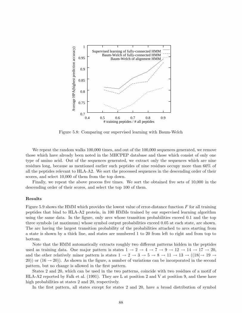
0.7

0.75

0.8

0.85

0.9

0.95

1

0.4 0.5 0.6 0.7 0.8 0.9

Ave

rage

HPA

(hig

hest

pre

dict

ion

accu

racy

)

# training peptides / # all peptides

Supervised learning of fully-connected HMMBaum-Welch of fully-connected HMM

Baum-Welch of alignment HMM

Figure 5.8: Comparing our supervised learning with Baum-Welch

We repeat the random walks 100,000 times, and out of the 100,000 sequences generated, we removethose which have already been noted in the MHCPEP database and those which consist of only onetype of amino acid. Out of the sequences generated, we extract only the sequences which are nineresidues long, because as mentioned earlier such peptides of nine residues occupy more than 60% ofall the peptides relevant to HLA-A2. We sort the processed sequences in the descending order of theirscores, and select 10,000 of them from the top down.

Finally, we repeat the above process five times. We sort the obtained five sets of 10,000 in thedescending order of their scores, and select the top 100 of them.

Results

Figure 5.9 shows the HMM which provides the lowest value of error-distance function F for all trainingpeptides that bind to HLA-A2 protein, in 100 HMMs trained by our supervised learning algorithmusing the same data. In the figure, only arcs whose transition probabilities exceed 0.1 and the topthree symbols (at maximum) whose symbol output probabilities exceed 0.05 at each state, are shown.The arc having the largest transition probability of the probabilities attached to arcs starting froma state is shown by a thick line, and states are numbered 1 to 20 from left to right and from top tobottom.

Note that the HMM automatically extracts roughly two different patterns hidden in the peptidesused as training data. One major pattern is states 1 → 2 → 4 → 7 → 9 → 12 → 14 → 17 → 20,and the other relatively minor pattern is states 1 → 2 → 3 → 5 → 8 → 11 → 13 → ((18(→ 19 →20)) or (16 → 20)). As shown in the figure, a number of variations can be incorporated in the secondpattern, but no change is allowed in the first pattern.

States 2 and 20, which can be used in the two patterns, coincide with two residues of a motif ofHLA-A2 reported by Falk et al. (1991). They are L at position 2 and V at position 9, and these havehigh probabilities at states 2 and 20, respectively.

In the first pattern, all states except for states 2 and 20, have a broad distribution of symbol

88

Initial state

0.99

Final state

L:0.12K:0.12A:0.11

0.99

0.89

0.91

0.69

0.88

0.17 0.43

0.56

0.770.20

0.55

1.00.24

1.0

0.10

1.0

0.20 0.19

0.61

0.54

0.89 0.96

0.86 0.60

0.830.13 0.63

0.87

0.32

0.140.11 0.40

L:0.64M:0.10I:0.05

L:0.11G:0.10P:0.09

G:0.12P:0.11R:0.08

L:0.12G:0.10F:0.09

P:0.10L:0.09G:0.09

P:0.13V:0.09L:0.09

G:0.13S:0.12L:0.10

V:0.57I:0.09Y:0.08

V:0.51R:0.24S:0.08

E:0.40F:0.35H:0.07

T:0.59N:0.12D:0.06

Q:0.73N:0.26

T:0.99

F:0.39D:0.32E:0.06

G:0.58W:0.17

I:0.86

L:0.75M:0.06

A:0.52K:0.16V:0.05

R:0.46T:0.28G:0.10

1 2

3

5

10

15

6

4 7 9 12 14 17 20

8 11 13 18

16 19

Figure 5.9: Main part of HMM representing peptides binding to HLA-A2

output probabilities, in which the largest probability value is at maximum 0.13. Furthermore, suchdistributions at states 4, 7, 9, 12, and 14 are similar to each other, and in them, G, L and P alwayshave relatively high probabilities. This result is consistent with a report by Sette et al. (1991), inwhich positions 3 to 5 in a HLA-A2 motif have the same amino acid propensity. This indicates,however, that neither the motif nor the first pattern can capture any distinct feature of this portion,and thus it will be difficult for them to accurately predict (or discriminate) peptides that bind toHLA-A2 protein.

On the other hand, the second pattern presents a more clear sequence pattern hidden in thetraining data. In particular, the transition of states 5 → 8 → 11 → 13 is connected by arcs, at anyof which a transition probability of 1.0 is attached, and this indicates that the transition is certainlyhidden in training peptide data. Actually, an MHC binding peptide experimentally found in Influenzamatrix protein (Gotch et al., 1988) contains the amino acid sequence FVFT, which can be generatedwith a high probability by this transition. The sequence is found in 49 of the total 472 peptides usedas training data, and this is one of the most frequent patterns in HLA-A2 binding peptides. Note thatthe sequence FVFT is found in a different position in each of the 49 training peptides. Out of the49 peptides, the number in which the sequence starts at the fourth, fifth, sixth, seventh and eighthposition is 3, 23, 20, 2 and 1, respectively.

We can find other frequent sequence patterns in the second pattern. For example, the longersequence LGFVFT, which can be generated by states 2 → 3 → 5 → 8 → 11 → 13 with a highprobability, is found in 36 peptides in the training data. Similarly, the sequence TLTV, which can begenerated by states 13 → 18 → 19 → 20, is in 33 peptides in training data. All frequent sequencepatterns, which are revealed by the HMM of Figure 5.9, are shown in Table 5.2. The patterns presentedin the table are those which are longer than three and which are found in more than 30 peptides inthe training data. If longer patterns, including those which satisfy the above requirement, are foundin more than 30 peptides, only the longest one of them is described. The table indicates that eachportion of the second pattern in the HMM captures hidden features in the training data.

Table 5.3 shows the top 100 peptides which were obtained by our random generation process

89

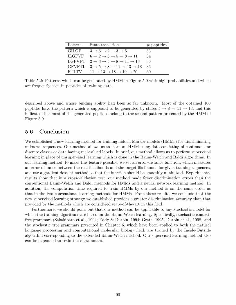
Patterns State transition # peptides

GILGF 3 → 6 → 2 → 3 → 5 33ILGFVF 6 → 2 → 3 → 5 → 8 → 11 34LGFVFT 2 → 3 → 5 → 8 → 11 → 13 36GFVFTL 3 → 5 → 8 → 11 → 13 → 18 36FTLTV 11 → 13 → 18 → 19 → 20 30

Table 5.2: Patterns which can be generated by HMM in Figure 5.9 with high probabilities and whichare frequently seen in peptides of training data

described above and whose binding ability had been so far unknown. Most of the obtained 100peptides have the pattern which is supposed to be generated by states 5 → 8 → 11 → 13, and thisindicates that most of the generated peptides belong to the second pattern presented by the HMM ofFigure 5.9.

5.6 Conclusion

We established a new learning method for training hidden Markov models (HMMs) for discriminatingunknown sequences. Our method allows us to learn an HMM using data consisting of continuous ordiscrete classes or data having real-valued labels. In brief, our method allows us to perform supervisedlearning in place of unsupervised learning which is done in the Baum-Welch and Baldi algorithms. Inour learning method, to make this feature possible, we set an error-distance function, which measuresan error-distance between the real likelihoods and the target likelihoods for given training sequences,and use a gradient descent method so that the function should be smoothly minimized. Experimentalresults show that in a cross-validation test, our method made fewer discrimination errors than theconventional Baum-Welch and Baldi methods for HMMs and a neural network learning method. Inaddition, the computation time required to train HMMs by our method is on the same order asthat in the two conventional learning methods for HMMs. From these results, we conclude that thenew supervised learning strategy we established provides a greater discrimination accuracy than thatprovided by the methods which are considered state-of-the-art in this field.

Furthermore, we should point out that our method can be applicable to any stochastic model forwhich the training algorithms are based on the Baum-Welch learning. Specifically, stochastic context-free grammars (Sakakibara et al., 1994; Eddy & Durbin, 1994; Grate, 1995; Durbin et al., 1998) andthe stochastic tree grammars presented in Chapter 6, which have been applied to both the naturallanguage processing and computational molecular biology field, are trained by the Inside-Outsidealgorithm corresponding to the extended Baum-Welch method. Our supervised learning method alsocan be expanded to train these grammars.

90

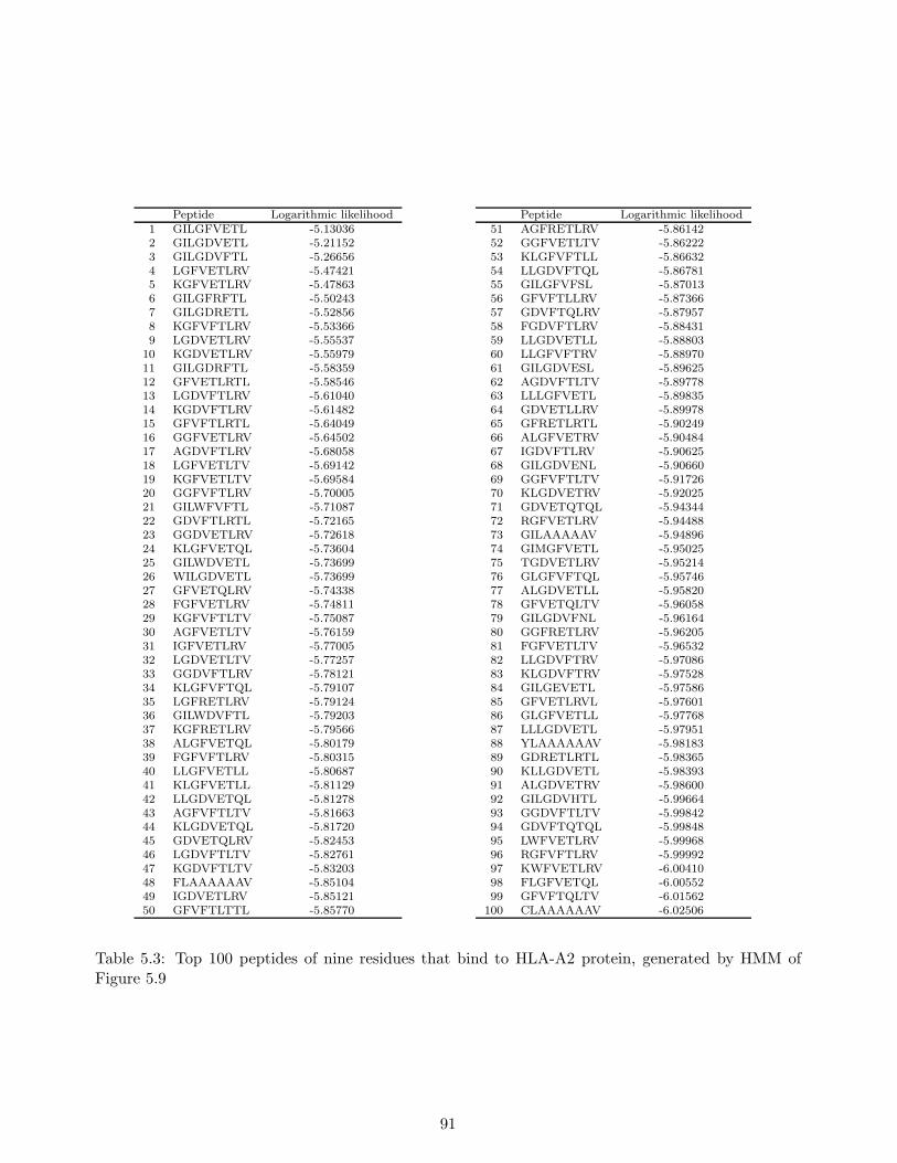
Peptide Logarithmic likelihood1 GILGFVETL -5.130362 GILGDVETL -5.211523 GILGDVFTL -5.266564 LGFVETLRV -5.474215 KGFVETLRV -5.478636 GILGFRFTL -5.502437 GILGDRETL -5.528568 KGFVFTLRV -5.533669 LGDVETLRV -5.55537

10 KGDVETLRV -5.5597911 GILGDRFTL -5.5835912 GFVETLRTL -5.5854613 LGDVFTLRV -5.6104014 KGDVFTLRV -5.6148215 GFVFTLRTL -5.6404916 GGFVETLRV -5.6450217 AGDVFTLRV -5.6805818 LGFVETLTV -5.6914219 KGFVETLTV -5.6958420 GGFVFTLRV -5.7000521 GILWFVFTL -5.7108722 GDVFTLRTL -5.7216523 GGDVETLRV -5.7261824 KLGFVETQL -5.7360425 GILWDVETL -5.7369926 WILGDVETL -5.7369927 GFVETQLRV -5.7433828 FGFVETLRV -5.7481129 KGFVFTLTV -5.7508730 AGFVETLTV -5.7615931 IGFVETLRV -5.7700532 LGDVETLTV -5.7725733 GGDVFTLRV -5.7812134 KLGFVFTQL -5.7910735 LGFRETLRV -5.7912436 GILWDVFTL -5.7920337 KGFRETLRV -5.7956638 ALGFVETQL -5.8017939 FGFVFTLRV -5.8031540 LLGFVETLL -5.8068741 KLGFVETLL -5.8112942 LLGDVETQL -5.8127843 AGFVFTLTV -5.8166344 KLGDVETQL -5.8172045 GDVETQLRV -5.8245346 LGDVFTLTV -5.8276147 KGDVFTLTV -5.8320348 FLAAAAAAV -5.8510449 IGDVETLRV -5.8512150 GFVFTLTTL -5.85770

Peptide Logarithmic likelihood51 AGFRETLRV -5.8614252 GGFVETLTV -5.8622253 KLGFVFTLL -5.8663254 LLGDVFTQL -5.8678155 GILGFVFSL -5.8701356 GFVFTLLRV -5.8736657 GDVFTQLRV -5.8795758 FGDVFTLRV -5.8843159 LLGDVETLL -5.8880360 LLGFVFTRV -5.8897061 GILGDVESL -5.8962562 AGDVFTLTV -5.8977863 LLLGFVETL -5.8983564 GDVETLLRV -5.8997865 GFRETLRTL -5.9024966 ALGFVETRV -5.9048467 IGDVFTLRV -5.9062568 GILGDVENL -5.9066069 GGFVFTLTV -5.9172670 KLGDVETRV -5.9202571 GDVETQTQL -5.9434472 RGFVETLRV -5.9448873 GILAAAAAV -5.9489674 GIMGFVETL -5.9502575 TGDVETLRV -5.9521476 GLGFVFTQL -5.9574677 ALGDVETLL -5.9582078 GFVETQLTV -5.9605879 GILGDVFNL -5.9616480 GGFRETLRV -5.9620581 FGFVETLTV -5.9653282 LLGDVFTRV -5.9708683 KLGDVFTRV -5.9752884 GILGEVETL -5.9758685 GFVETLRVL -5.9760186 GLGFVETLL -5.9776887 LLLGDVETL -5.9795188 YLAAAAAAV -5.9818389 GDRETLRTL -5.9836590 KLLGDVETL -5.9839391 ALGDVETRV -5.9860092 GILGDVHTL -5.9966493 GGDVFTLTV -5.9984294 GDVFTQTQL -5.9984895 LWFVETLRV -5.9996896 RGFVFTLRV -5.9999297 KWFVETLRV -6.0041098 FLGFVETQL -6.0055299 GFVFTQLTV -6.01562

100 CLAAAAAAV -6.02506

Table 5.3: Top 100 peptides of nine residues that bind to HLA-A2 protein, generated by HMM ofFigure 5.9

91

Chapter 6

Discovering Common β-sheets withStochastic Tree Grammar Learning

6.1 Introduction

Protein is made of a sequence of amino acids which is folded into a 3-dimensional structure. Proteinsecondary structures are relatively small groups of protein structures exhibiting certain notable andregular characteristics, which function as intermediate building blocks of the overall protein structure,and can be classified into three types; α-helix, β-sheet, and others. We established a new methodfor predicting protein secondary structure of a given amino acid sequence, based on a classificationrule automatically learned from a relatively small database of sequences whose secondary structureshave been experimentally determined (Mamitsuka & Abe, 1994a; Abe & Mamitsuka, 1997, 1994).Among the above three types, we concentrated on the problem of predicting β-sheet regions in a givenamino acid sequence. Our strategy receives as input amino acid sequences known to contain β-sheetregions, and train the probability parameters of a certain type of stochastic tree grammar so that itsdistribution best approximates the patterns of the input sample. Some of the rules in the grammarare intended a priori for generating β-sheet regions and others for non-β-sheets. After training, themethod is given a sequence of amino acids with unknown secondary structure, and predicts accordingto which regions are generated by the β-sheet rules, in the most likely parse for the input sequence.

The problem of predicting protein structures from their amino acid sequences is probably the singlemost important problem in computational molecular biology with immense scientific significance andbroad engineering applications. Since the early 1990s, increasing attention has been given to the three-dimensional structural prediction methods which attempt to predict the entire protein structure, suchas homology modeling (c.f. Sanchez & Sali, 1997) and remote homology modeling (c.f. Jones, 1997).These methods are based on alignment/scoring of the test sequence against sequences with knownstructure, and therefore are not effective for those sequences having less than 25% sequence similarityto the training sequences (Sander & Schneider, 1991). At the other end of the spectrum is theprotein secondary structure prediction approach, which is general in the sense that it does not relyon alignment with sequences with known structure and hence can be applied on sequences havinglittle or no sequence similarity, but provides less information. The present chapter aims at providinga general method which can be applied to sequences with less than 25% sequence similarity, and yetprovides more structural information.

The classical secondary structure prediction problem is the problem of determining which regionsin a given amino acid sequence correspond to each of the above three categories (Barton, 1995; Cuff& Barton, 1999). At the midst of 1990s, there were several approaches for the prediction of α-helix

92

regions using machine learning techniques which achieved moderate success. The prediction rates ofapproximate 80 percent, varying depending on the exact conditions of experimentation, achieved bysome of these methods (Mamitsuka & Yamanishi, 1992, 1995; Rost & Sander, 1993b). The problemof predicting β-sheet regions, however, was not treated at a comparable level. This asymmetry canbe attributed to the property of β-sheets that their structures typically range over several discontin-uous sections in an amino acid sequence, whereas the structures of α-helix are continuous and theirdependency patterns are more regular.

To cope with this difficulty, we defined a certain family of stochastic tree grammars whose expres-sive powers exceed not only that of hidden Markov models (HMMs), but also stochastic context freegrammars (SCFGs). SCFGs are used extensively in speech recognition, and have been introduced tocomputational molecular biology (Sakakibara et al., 1994; Durbin et al., 1998). Context free grammarsare not powerful enough to capture the kind of long-distance dependencies exhibited by the aminoacid sequences of β-sheet regions. This is because the β-sheet regions exhibit both the ‘anti-parallel’dependency (of the type abccba), and ‘parallel’ dependency (of the type abcabc), and moreover, var-ious combinations of them (as, for example, in abccbaabcabc). The class of stochastic tree grammarswhich we will define in this chapter, the stochastic ranked node rewriting grammar (SRNRG), is one ofthe rare families of grammatical systems that have both enough expressive power to cope with all ofthese dependencies and at the same time enjoy relatively efficient parsability and learnability. Searls(1993) noted that the language of β-sheets is beyond context free and suggested that they are indexedlanguages. Indexed languages are not recognizable in polynomial time, however, and hence indexedgrammars are not useful for our purpose. RNRG falls between them and appears to be just what weneed.

The ranked node rewriting grammars (RNRGs) were briefly introduced in the context of compu-tationally efficient learnability of grammars by Abe (Abe, 1988), but its formal properties as well asbasic methods such as parsing and learning algorithms were left for future research. The discoveryof RNRGs was inspired by the pioneering work of Joshi et al (see e.g. Joshi, Levy, & Takahashi,1975; Vijay-Shanker & Joshi, 1985) on a tree grammatical system for natural language called ‘TreeAdjoining Grammars’ (or TAGs for short), but RNRGs generalizes TAGs just in a way that is suitedto capture the type of dependencies present in the sequences in β-sheet regions. For example, TAGcan handle a single parallel dependency, which cannot be handled by CFG, but cannot deal with acomplicated combination of anti-parallel and parallel dependencies. All of such dependencies can becaptured by some members of the RNRG family.

The learning algorithm we established is an extension of the ‘Inside-Outside’ algorithm for thestochastic context free grammars (Jelinik, Lafferty, & Mercer, 1990), and is also related to the ex-tension of the Inside-Outside algorithm developed for the stochastic tree adjoining grammars bySchabes (1992). These are extended versions of the Baum-Welch algorithm for HMMs and all iter-ative algorithms guaranteed to find a local optimal for the maximum likelihood settings of the ruleapplication probabilities. Perhaps the most serious difficulty with our method is the extensive com-putation required by the parsing and learning algorithms. The computational requirement of thelearning algorithm is brought down drastically by using the so-called ‘bracketing’ technique. That is,when training an SRNRG fragment corresponding to a certain β-sheet region, rather than feeding theentire input sequence to the learning algorithm, the concatenation of just those substrings of the inputsequence which correspond to the β-sheet region is fed to the learning algorithm. In contrast, theparsing algorithm must process the entire input string, as it clearly does not know in advance whichsubstrings in the input sequence correspond to the β-sheet region. Hence most of the computationalrequirement is concentrated on the parsing algorithm.

In order to reduce the computational requirement of the parsing algorithm, we restricted the form

93

of grammars to a certain subclass of SRNRG which we call linear SRNRG and devised a simpler andfaster algorithm for the subclass. This subclass is obtained by placing the restriction that the righthand side of any rewriting rule contains exactly one occurrence of a non-terminal, excepting lexicalnon-terminals. This significantly simplifies the parsing and learning algorithms as the computationof each entry in the parsing table becomes much simpler. In addition, we parallelized our parsingalgorithm and implemented it on a 32-processor CM-5 parallel machine. We were able to obtain anearly linear speed-up, and were able to predict the structure of a test sequence of length 100 in abouta minute, whereas the same task took our sequential algorithm almost 30 minutes.

We also established a method of reducing the alphabet size (i.e. the number of amino acids) byclustering them using MDL (Minimum Description Length) approximation (Rissanen, 1989) and theirphysico-chemical properties, gradually through the iterations of the learning algorithm. The physico-chemical properties we used are the molecular weight and the hydrophobicity, which were used inChapter 3 for predicting α-helix regions. That is, after each iteration of the learning algorithm, weattempted to merge a small number of amino acids, if doing so reduces the total description lengthusing the likelihood calculation performed up to that point.

As a preliminary experiment, we first used three toxins which have a common 3-dimensionalstructure shown in Figure 6.4, but each of three has less than 25% pairwise sequence similarity. Theresults obtained indicate that our method is able to capture and generalize the type of long-distancedependencies that characterize β-sheets of the toxins. Using an SRNRG trained by data for one ofthree toxins, our method was actually able to predict the location and structure of β-sheets in theother two toxins. With the training sequences and the test sequences having less than 25% sequenceidentity, such a prediction problem belongs to what is sometimes referred to in the literature as the‘Twilight Zone’ (Doolittle et al., 1986), where alignment is no longer effective.

Then, we conducted a large-scale experiment in which proteins used for training and those fortesting not only have almost no sequence similarity, but their structures have no apparent relationship.In the experiment, we restricted our attention on the β-sheet regions that can be expressed usingrank 1 linear SRNRGs, which we call rank 1 four-strand patterns or rank 1 four-strand β-sheets.Furthermore, for simplicity, we write four-strand patterns for rank 1 four-strand patterns. As trainingdata we used all the sequences (satisfying a certain weak condition), listed in PDB SELECT 25% list(Hoboem et al., 1992), a database containing sequences of protein with known structure possessing atmost 25% sequence similarity with one another. For each one of these sequences, we enhanced it bythe set of aligned sequences listed in the HSSP (Homology-derived Secondary Structure of Proteins)(Sander & Schneider, 1991) for it, as is done by a number of secondary structure prediction methods(Rost & Sander, 1993a; Mamitsuka & Yamanishi, 1995). As test sequences, we took all sequences inPDB SELECT 25% list of length at most 200, excluding the training sequences themselves, containingrelevant types of four-strand patterns. The above process translates to saying that we used essentiallyall data that are currently available, and hence without any bias. The prediction was made accordingto the location and structure of the most likely analysis given by these grammar fragments, exceptthe fragment trained on sequences that have less than 25% sequence similarity to the test sequence,thereby ensuring that the prediction could not be done easily by homology modeling.

The results of our experiment indicate that the prediction made by our method on the approximatelocations and structures of arbitrary rank 1 four-strand β-sheets is statistically significant, althoughits predictive accuracy is not yet at a satisfactory level. Our method was able to actually predictthe structure of a couple of rank 1 four-strand β-sheets approximately correctly, based on stochasticgrammar fragments trained on sequences of proteins that are very different from that of the testsequence, thus discovering a hitherto unnoticed similarity that exists between local structures ofapparently unrelated proteins. Also, in the course of the experiments, it was observed that the

94

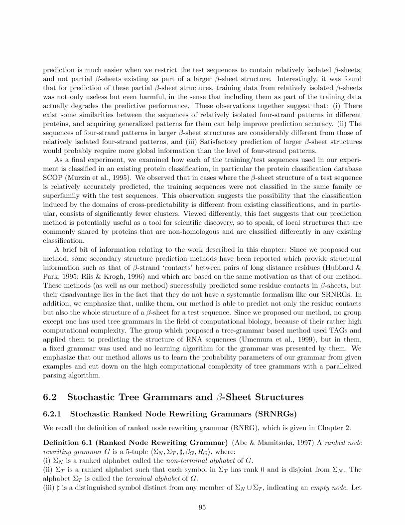
prediction is much easier when we restrict the test sequences to contain relatively isolated β-sheets,and not partial β-sheets existing as part of a larger β-sheet structure. Interestingly, it was foundthat for prediction of these partial β-sheet structures, training data from relatively isolated β-sheetswas not only useless but even harmful, in the sense that including them as part of the training dataactually degrades the predictive performance. These observations together suggest that: (i) Thereexist some similarities between the sequences of relatively isolated four-strand patterns in differentproteins, and acquiring generalized patterns for them can help improve prediction accuracy. (ii) Thesequences of four-strand patterns in larger β-sheet structures are considerably different from those ofrelatively isolated four-strand patterns, and (iii) Satisfactory prediction of larger β-sheet structureswould probably require more global information than the level of four-strand patterns.

As a final experiment, we examined how each of the training/test sequences used in our experi-ment is classified in an existing protein classification, in particular the protein classification databaseSCOP (Murzin et al., 1995). We observed that in cases where the β-sheet structure of a test sequenceis relatively accurately predicted, the training sequences were not classified in the same family orsuperfamily with the test sequences. This observation suggests the possibility that the classificationinduced by the domains of cross-predictability is different from existing classifications, and in partic-ular, consists of significantly fewer clusters. Viewed differently, this fact suggests that our predictionmethod is potentially useful as a tool for scientific discovery, so to speak, of local structures that arecommonly shared by proteins that are non-homologous and are classified differently in any existingclassification.

A brief bit of information relating to the work described in this chapter: Since we proposed ourmethod, some secondary structure prediction methods have been reported which provide structuralinformation such as that of β-strand ‘contacts’ between pairs of long distance residues (Hubbard &Park, 1995; Riis & Krogh, 1996) and which are based on the same motivation as that of our method.These methods (as well as our method) successfully predicted some residue contacts in β-sheets, buttheir disadvantage lies in the fact that they do not have a systematic formalism like our SRNRGs. Inaddition, we emphasize that, unlike them, our method is able to predict not only the residue contactsbut also the whole structure of a β-sheet for a test sequence. Since we proposed our method, no groupexcept one has used tree grammars in the field of computational biology, because of their rather highcomputational complexity. The group which proposed a tree-grammar based method used TAGs andapplied them to predicting the structure of RNA sequences (Umemura et al., 1999), but in them,a fixed grammar was used and no learning algorithm for the grammar was presented by them. Weemphasize that our method allows us to learn the probability parameters of our grammar from givenexamples and cut down on the high computational complexity of tree grammars with a parallelizedparsing algorithm.

6.2 Stochastic Tree Grammars and β-Sheet Structures

6.2.1 Stochastic Ranked Node Rewriting Grammars (SRNRGs)

We recall the definition of ranked node rewriting grammar (RNRG), which is given in Chapter 2.

Definition 6.1 (Ranked Node Rewriting Grammar) (Abe & Mamitsuka, 1997) A ranked noderewriting grammar G is a 5-tuple 〈ΣN ,ΣT , ], βG, RG〉, where:(i) ΣN is a ranked alphabet called the non-terminal alphabet of G.(ii) ΣT is a ranked alphabet such that each symbol in ΣT has rank 0 and is disjoint from ΣN . Thealphabet ΣT is called the terminal alphabet of G.(iii) ] is a distinguished symbol distinct from any member of ΣN ∪ΣT , indicating an empty node. Let

95

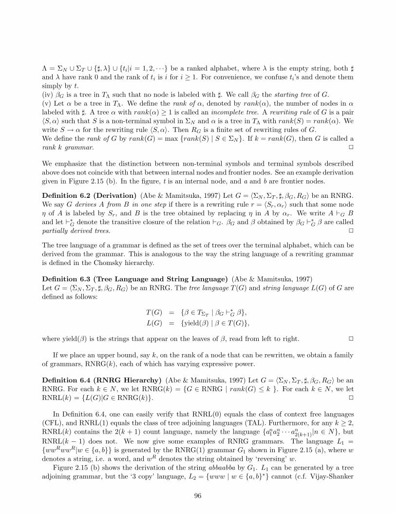
Λ = ΣN ∪ ΣT ∪ {], λ} ∪ {ti|i = 1, 2, · · ·} be a ranked alphabet, where λ is the empty string, both ]and λ have rank 0 and the rank of ti is i for i ≥ 1. For convenience, we confuse ti’s and denote themsimply by t.(iv) βG is a tree in TΛ such that no node is labeled with ]. We call βG the starting tree of G.(v) Let α be a tree in TΛ. We define the rank of α, denoted by rank(α), the number of nodes in αlabeled with ]. A tree α with rank(α) ≥ 1 is called an incomplete tree. A rewriting rule of G is a pair〈S, α〉 such that S is a non-terminal symbol in ΣN and α is a tree in TΛ with rank(S) = rank(α). Wewrite S → α for the rewriting rule 〈S, α〉. Then RG is a finite set of rewriting rules of G.We define the rank of G by rank(G) = max {rank(S) | S ∈ ΣN}. If k = rank(G), then G is called arank k grammar. 2

We emphasize that the distinction between non-terminal symbols and terminal symbols describedabove does not coincide with that between internal nodes and frontier nodes. See an example derivationgiven in Figure 2.15 (b). In the figure, t is an internal node, and a and b are frontier nodes.

Definition 6.2 (Derivation) (Abe & Mamitsuka, 1997) Let G = 〈ΣN ,ΣT , ], βG, RG〉 be an RNRG.We say G derives A from B in one step if there is a rewriting rule r = 〈Sr, αr〉 such that some nodeη of A is labeled by Sr, and B is the tree obtained by replacing η in A by αr. We write A `G Band let `∗

G denote the transitive closure of the relation `G. βG and β obtained by βG `∗G β are called

partially derived trees. 2

The tree language of a grammar is defined as the set of trees over the terminal alphabet, which can bederived from the grammar. This is analogous to the way the string language of a rewriting grammaris defined in the Chomsky hierarchy.

Definition 6.3 (Tree Language and String Language) (Abe & Mamitsuka, 1997)Let G = 〈ΣN ,ΣT , ], βG, RG〉 be an RNRG. The tree language T (G) and string language L(G) of G aredefined as follows:

T (G) = {β ∈ TΣT| βG `∗

G β},

L(G) = {yield(β) | β ∈ T (G)},

where yield(β) is the strings that appear on the leaves of β, read from left to right. 2

If we place an upper bound, say k, on the rank of a node that can be rewritten, we obtain a familyof grammars, RNRG(k), each of which has varying expressive power.

Definition 6.4 (RNRG Hierarchy) (Abe & Mamitsuka, 1997) Let G = 〈ΣN ,ΣT , ], βG, RG〉 be anRNRG. For each k ∈ N , we let RNRG(k) = {G ∈ RNRG | rank(G) ≤ k }. For each k ∈ N , we letRNRL(k) = {L(G)|G ∈ RNRG(k)}. 2

In Definition 6.4, one can easily verify that RNRL(0) equals the class of context free languages(CFL), and RNRL(1) equals the class of tree adjoining languages (TAL). Furthermore, for any k ≥ 2,RNRL(k) contains the 2(k + 1) count language, namely the language {an

1an2 · · · an

2(k+1)|n ∈ N}, but

RNRL(k − 1) does not. We now give some examples of RNRG grammars. The language L1 ={wwRwwR|w ∈ {a, b}} is generated by the RNRG(1) grammar G1 shown in Figure 2.15 (a), where wdenotes a string, i.e. a word, and wR denotes the string obtained by ‘reversing’ w.

Figure 2.15 (b) shows the derivation of the string abbaabba by G1. L1 can be generated by a treeadjoining grammar, but the ‘3 copy’ language, L2 = {www | w ∈ {a, b}∗} cannot (c.f. Vijay-Shanker

96

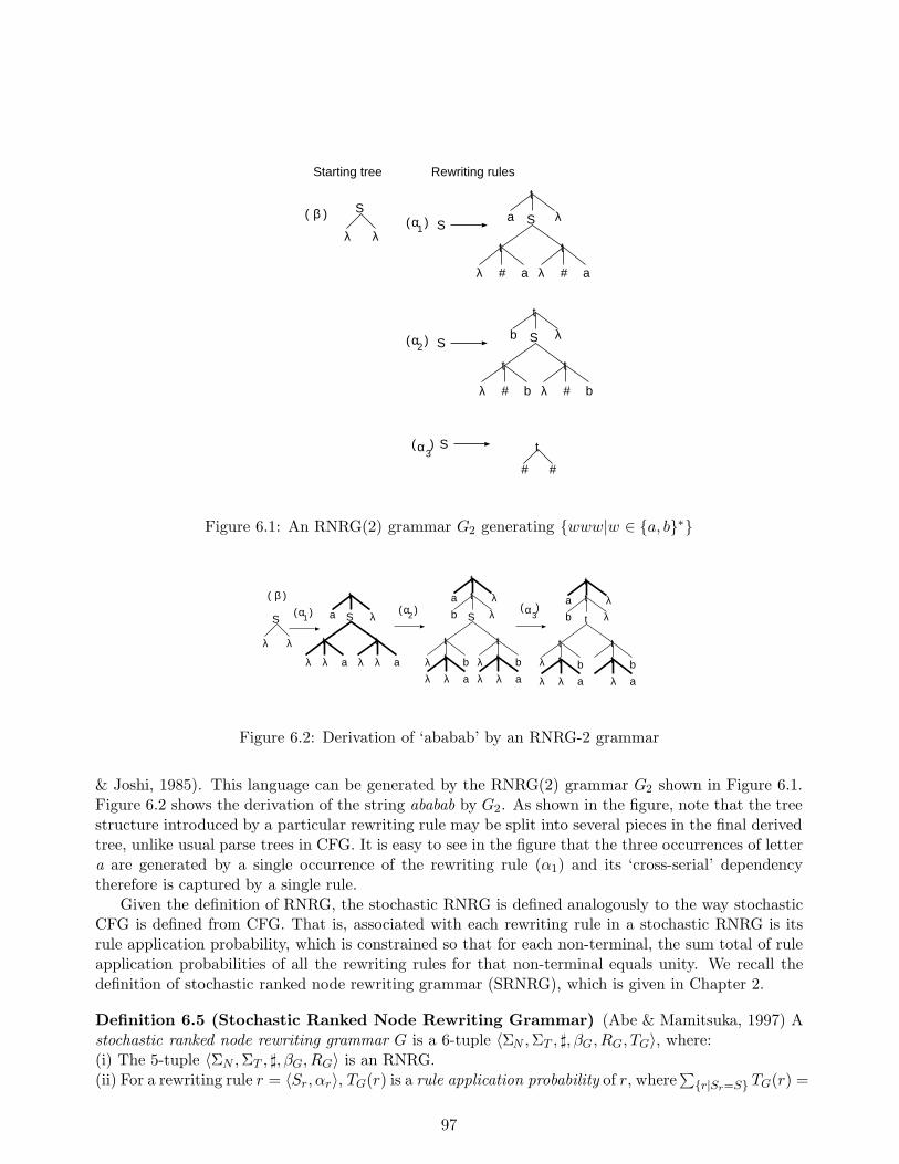
Starting tree

( )

Rewriting rules

S( )

( )

( )

S Sλ

βα

α

α

a

a

S

S

1

2

3

t

tλ

t

a

Sb

b

t

t t

b

t

λ

λλ

λ

λλ

# #

##

# #

Figure 6.1: An RNRG(2) grammar G2 generating {www|w ∈ {a, b}∗}

( )

S( ) ( ) ( )

S

λ

βα α αa

a

1 2 3

t

tλ t

a

Sb

b

t

t t

b

a

λ λa

t t

aλ λ

b

b

t

t t

b

a

t

a

t t

aλ λ

t

t

λλ

λ

λλλλ λ

λλ

λ

λλ

Figure 6.2: Derivation of ‘ababab’ by an RNRG-2 grammar

& Joshi, 1985). This language can be generated by the RNRG(2) grammar G2 shown in Figure 6.1.Figure 6.2 shows the derivation of the string ababab by G2. As shown in the figure, note that the treestructure introduced by a particular rewriting rule may be split into several pieces in the final derivedtree, unlike usual parse trees in CFG. It is easy to see in the figure that the three occurrences of lettera are generated by a single occurrence of the rewriting rule (α1) and its ‘cross-serial’ dependencytherefore is captured by a single rule.

Given the definition of RNRG, the stochastic RNRG is defined analogously to the way stochasticCFG is defined from CFG. That is, associated with each rewriting rule in a stochastic RNRG is itsrule application probability, which is constrained so that for each non-terminal, the sum total of ruleapplication probabilities of all the rewriting rules for that non-terminal equals unity. We recall thedefinition of stochastic ranked node rewriting grammar (SRNRG), which is given in Chapter 2.

Definition 6.5 (Stochastic Ranked Node Rewriting Grammar) (Abe & Mamitsuka, 1997) Astochastic ranked node rewriting grammar G is a 6-tuple 〈ΣN ,ΣT , ], βG, RG, TG〉, where:(i) The 5-tuple 〈ΣN ,ΣT , ], βG, RG〉 is an RNRG.(ii) For a rewriting rule r = 〈Sr, αr〉, TG(r) is a rule application probability of r, where

∑

{r|Sr=S} TG(r) =

97

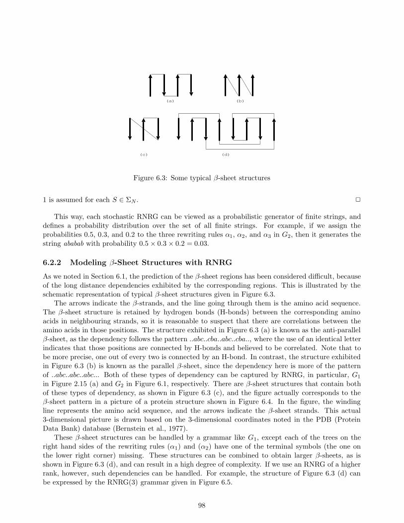
(a) (b)

(d)(c)

Figure 6.3: Some typical β-sheet structures

1 is assumed for each S ∈ ΣN . 2

This way, each stochastic RNRG can be viewed as a probabilistic generator of finite strings, anddefines a probability distribution over the set of all finite strings. For example, if we assign theprobabilities 0.5, 0.3, and 0.2 to the three rewriting rules α1, α2, and α3 in G2, then it generates thestring ababab with probability 0.5 × 0.3 × 0.2 = 0.03.

6.2.2 Modeling β-Sheet Structures with RNRG

As we noted in Section 6.1, the prediction of the β-sheet regions has been considered difficult, becauseof the long distance dependencies exhibited by the corresponding regions. This is illustrated by theschematic representation of typical β-sheet structures given in Figure 6.3.

The arrows indicate the β-strands, and the line going through them is the amino acid sequence.The β-sheet structure is retained by hydrogen bonds (H-bonds) between the corresponding aminoacids in neighbouring strands, so it is reasonable to suspect that there are correlations between theamino acids in those positions. The structure exhibited in Figure 6.3 (a) is known as the anti-parallelβ-sheet, as the dependency follows the pattern ..abc..cba..abc..cba.., where the use of an identical letterindicates that those positions are connected by H-bonds and believed to be correlated. Note that tobe more precise, one out of every two is connected by an H-bond. In contrast, the structure exhibitedin Figure 6.3 (b) is known as the parallel β-sheet, since the dependency here is more of the patternof ..abc..abc..abc... Both of these types of dependency can be captured by RNRG, in particular, G1

in Figure 2.15 (a) and G2 in Figure 6.1, respectively. There are β-sheet structures that contain bothof these types of dependency, as shown in Figure 6.3 (c), and the figure actually corresponds to theβ-sheet pattern in a picture of a protein structure shown in Figure 6.4. In the figure, the windingline represents the amino acid sequence, and the arrows indicate the β-sheet strands. This actual3-dimensional picture is drawn based on the 3-dimensional coordinates noted in the PDB (ProteinData Bank) database (Bernstein et al., 1977).

These β-sheet structures can be handled by a grammar like G1, except each of the trees on theright hand sides of the rewriting rules (α1) and (α2) have one of the terminal symbols (the one onthe lower right corner) missing. These structures can be combined to obtain larger β-sheets, as isshown in Figure 6.3 (d), and can result in a high degree of complexity. If we use an RNRG of a higherrank, however, such dependencies can be handled. For example, the structure of Figure 6.3 (d) canbe expressed by the RNRG(3) grammar given in Figure 6.5.

98

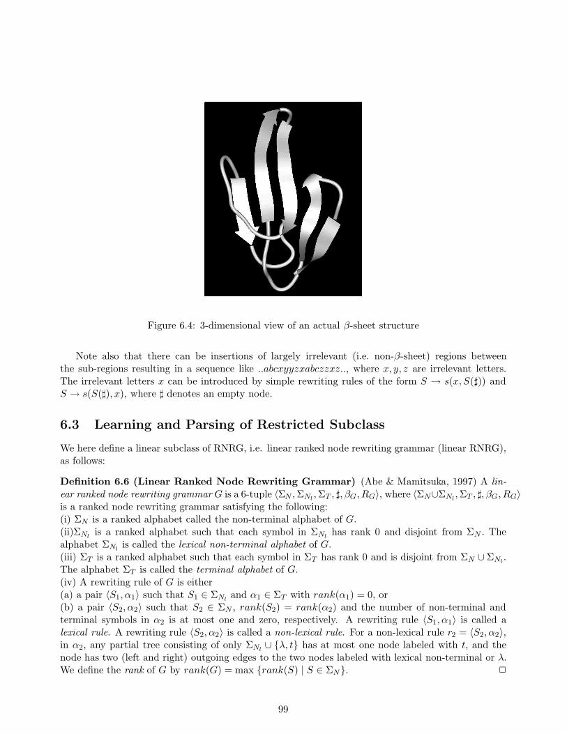
Figure 6.4: 3-dimensional view of an actual β-sheet structure

Note also that there can be insertions of largely irrelevant (i.e. non-β-sheet) regions betweenthe sub-regions resulting in a sequence like ..abcxyyzxabczzxz.., where x, y, z are irrelevant letters.The irrelevant letters x can be introduced by simple rewriting rules of the form S → s(x, S(])) andS → s(S(]), x), where ] denotes an empty node.

6.3 Learning and Parsing of Restricted Subclass

We here define a linear subclass of RNRG, i.e. linear ranked node rewriting grammar (linear RNRG),as follows:

Definition 6.6 (Linear Ranked Node Rewriting Grammar) (Abe & Mamitsuka, 1997) A lin-ear ranked node rewriting grammar G is a 6-tuple 〈ΣN ,ΣNl

,ΣT , ], βG, RG〉, where 〈ΣN∪ΣNl,ΣT , ], βG, RG〉

is a ranked node rewriting grammar satisfying the following:(i) ΣN is a ranked alphabet called the non-terminal alphabet of G.(ii)ΣNl

is a ranked alphabet such that each symbol in ΣNlhas rank 0 and disjoint from ΣN . The

alphabet ΣNlis called the lexical non-terminal alphabet of G.

(iii) ΣT is a ranked alphabet such that each symbol in ΣT has rank 0 and is disjoint from ΣN ∪ ΣNl.

The alphabet ΣT is called the terminal alphabet of G.(iv) A rewriting rule of G is either(a) a pair 〈S1, α1〉 such that S1 ∈ ΣNl

and α1 ∈ ΣT with rank(α1) = 0, or(b) a pair 〈S2, α2〉 such that S2 ∈ ΣN , rank(S2) = rank(α2) and the number of non-terminal andterminal symbols in α2 is at most one and zero, respectively. A rewriting rule 〈S1, α1〉 is called alexical rule. A rewriting rule 〈S2, α2〉 is called a non-lexical rule. For a non-lexical rule r2 = 〈S2, α2〉,in α2, any partial tree consisting of only ΣNl

∪ {λ, t} has at most one node labeled with t, and thenode has two (left and right) outgoing edges to the two nodes labeled with lexical non-terminal or λ.We define the rank of G by rank(G) = max {rank(S) | S ∈ ΣN}. 2

99

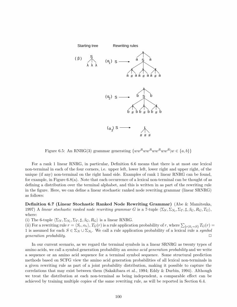
Starting tree

( )

Rewriting rules

S( )

( )

( )

S Sλ

βα

α

α

a

a

S

S

1

2

3

t

tλ

t

a

λ

t

t

a a a a a

Sb

b

t

t t

b

t

b b b b b

# ##

# # #

###

Figure 6.5: An RNRG(3) grammar generating {wwRwwRwwRwwR|w ∈ {a, b}}

For a rank 1 linear RNRG, in particular, Definition 6.6 means that there is at most one lexicalnon-terminal in each of the four corners, i.e. upper left, lower left, lower right and upper right, of theunique (if any) non-terminal on the right hand side. Examples of rank 1 linear RNRG can be found,for example, in Figure 6.8(a). Note that each occurrence of a lexical non-terminal can be thought of asdefining a distribution over the terminal alphabet, and this is written in as part of the rewriting rulein the figure. Here, we can define a linear stochastic ranked node rewriting grammar (linear SRNRG)as follows:

Definition 6.7 (Linear Stochastic Ranked Node Rewriting Grammar) (Abe & Mamitsuka,1997) A linear stochastic ranked node rewriting grammar G is a 7-tuple 〈ΣN ,ΣNl

,ΣT , ], βG, RG, TG〉,where:(i) The 6-tuple 〈ΣN ,ΣNl

,ΣT , ], βG, RG〉 is a linear RNRG.(ii) For a rewriting rule r = 〈Sr, αr〉, TG(r) is a rule application probability of r, where

∑

{r|Sr=S} TG(r) =1 is assumed for each S ∈ ΣN ∪ ΣNl

. We call a rule application probability of a lexical rule a symbolgeneration probability. 2

In our current scenario, as we regard the terminal symbols in a linear SRNRG as twenty types ofamino acids, we call a symbol generation probability an amino acid generation probability and we writea sequence or an amino acid sequence for a terminal symbol sequence. Some structural predictionmethods based on SCFG view the amino acid generation probabilities of all lexical non-terminals ina given rewriting rule as part of a joint probability distribution, making it possible to capture thecorrelations that may exist between them (Sakakibara et al., 1994; Eddy & Durbin, 1994). Althoughwe treat the distribution at each non-terminal as being independent, a comparable effect can beachieved by training multiple copies of the same rewriting rule, as will be reported in Section 6.4.

100

With the linear constraints described in Definition 6.6, the parsing and learning algorithms forSRNRGs can be significantly simplified. For a general SRNRG of rank k, the entries in the tableused in the extended Inside-Outside algorithm (indexed by a 2(k + 1)-dimensional array) need to benode-addresses of the tree structures appearing in the rewriting rules of the grammar, paired withtheir probabilities of generating the designated sections of the input string. With the linear SRNRGin Definition 6.6, it suffices to place just the non-terminals (and the rewriting rules also in the caseof parsing) in the table entries, paired with their probabilities. These constraints also imply that the‘yield’ of any particular rewriting rule consists of at most 2(k + 1) sections in the input string, andhence can be found in ‘one shot.’ Note that in a general SRNRG, there is no a priori limit on howmany different sections the yield of any given rewriting rule body can be divided into (though it isbounded above by a constant depending on the grammar) and thus they cannot be found in ‘one shot’even if all the 2(k + 1) tuples of substrings of the input string are inspected.

6.3.1 Learning Algorithm for Linear SRNRG

Our novel learning algorithm is an extension of the Inside-Outside algorithm for SCFG, which isitself an extension of the Baum-Welch algorithm (or the Forward-Backward algorithm) for the HiddenMarkov Models. All of these algorithms are local optimization algorithms for the maximum likelihoodsettings of the rule application probabilities in the input model or grammar. It is well-known (seeLevinson, Rabiner, & Sondhi, 1983) that this Baum-Welch re-estimation algorithm is guaranteedto increase the likelihood given to the input sequences, and hence iterative applications of this re-estimation result in a local optimization algorithm.

For both SCFG and linear SRNRG, the forward probability and the backward probability aregeneralized as inside probability and outside probability. The algorithm we will describe is for rank 1linear SRNRG. We define the inside probability and outside probability as follows:

Definition 6.8 (Inside Probability) (Abe & Mamitsuka, 1997) Let G = 〈ΣN ,ΣNl,ΣT , ], βG, RG, TG〉

be a rank 1 linear SRNRG. For a terminal symbol sequence σ = σ1 · · · σn, a non-terminal symbolS ∈ ΣN and 0 ≤ i ≤ j ≤ k ≤ l ≤ n, the inside probability Inσ[S, i, j, k, l] is the probability that thepartially derived tree whose two discontinuous yields match σi+1 · · · σj and σk+1 · · · σl, contains S asthe unique non-terminal. 2

Definition 6.9 (Outside Probability) (Abe & Mamitsuka, 1997) Let G = 〈ΣN ,ΣNl,ΣT , ], βG, RG, TG〉

be a rank 1 linear SRNRG. For a terminal symbol sequence σ = σ1 · · · σn, a non-terminal symbolS ∈ ΣN and 0 ≤ i ≤ j ≤ k ≤ l ≤ n, the outside probability Outσ[S, i, j, k, l] is the probability thatthe partially derived tree whose three discontinuous yields match σ1 · · · σi, σj+1 · · · σk and σl+1 · · · σn,contains S as the unique non-terminal. 2

Now we show how the inside and outside probabilities are calculated. The inside probabilitiesat arbitrary index (i, j, k, l) can be defined recursively solely in terms of the inside probabilities of‘smaller’ intervals, so they can be calculated as long as the inside probabilities at those (i′, j′, k′, l′)such that (j′ − i′) + (l′ − k′) < (j − i) + (l − k) have already been calculated. The looping used inthe procedure for calculating the inside probabilities exhibited below ensures that this condition issatisfied.

Now let G = 〈ΣN ,ΣNl,ΣT , ], βG, RG, TG〉 be a given rank 1 linear SRNRG. For a non-lexical rule

r = 〈L(r), αr〉, let R(r) be the unique non-terminal on the right hand side of r, nrf (f = 1, · · · , 4) be

the number (0 or 1) of lexical non-terminal symbols at each of the four corners (upper left, lower left,lower right, and upper right) in the αr, Sr

f be the (if any) lexical non-terminal symbols at a corner

101

f = 1, 2, 3, 4, P rf (a) be the symbol generation probability of a lexical rule Sr

f → a in a corner f . Notethat for a non-lexical rule r and a lexical rule r′ = 〈Sr

f , a〉, TG(r′) = P rf (a).

Algorithm 6.10 (Inside) (Abe & Mamitsuka, 1997)input: rank 1 linear SRNRG G = 〈ΣN ,ΣNl

,ΣT , ], βG, RG, TG〉 and a terminal symbol sequence σ oflength noutput: inside probabilities

For i := n to 0For j := i to nFor k := n to jFor l := k to nFor S ∈ ΣN

Inσ[S, i, j, k, l] =∑

{r∈RG|L(r)=S}{ TG(r) · Inσ[R(r), i+nr

1, j−nr2, k+nr

3, l−nr4] ·

(P r1 (σi+1))

nr1(P r

2 (σj))nr

2(P r3 (σk+1))

nr3(P r

4 (σl))nr

4 }

2

The outside probabilities can be calculated in a similar fashion, as shown below.

Algorithm 6.11 (Outside) (Abe & Mamitsuka, 1997)input: rank 1 linear SRNRG G = 〈ΣN ,ΣNl

,ΣT , ], βG, RG, TG〉 and a terminal symbol sequence σ oflength noutput: outside probabilities

For i := 0 to nFor j := n to iFor k := j to nFor l := n to kFor S ∈ ΣN

Outσ[S, i, j, k, l] =∑

{r∈RG|R(r)=S}{ TG(r) · Outσ[L(r), i−nr

1, j+nr2, k−nr

3, l+nr4] ·

(P r1 (σi))

nr1(P r

2 (σj+1))nr

2(P r3 (σk))

nr3(P r

4 (σl+1))nr

4 }

2

Definition 6.12 (Pr) (Abe & Mamitsuka, 1997) Let G = 〈ΣN ,ΣNl,ΣT , ], βG, RG, TG〉 be a rank

1 linear SRNRG. For a sequence σ = σ1 · · · σn, a non-lexical rule r and 0 ≤ i ≤ j ≤ k ≤ l ≤ n,Prσ[r, i, j, k, l] is the probability that σ is generated by G, using r at the four positions (i, j, k, l) of σ.2

Using the inside and outside probabilities, the Prσ[r, i, j, k, l] can be calculated as follows:

Prσ[r, i, j, k, l] =Outσ[L(r), i, j, k, l] · Inσ[R(r), i+nr1, j−nr

2, k+nr3, l−nr

4] · TG(r) ·

(P r1 (σi+1))

nr1(P r

2 (σj))nr

2(P r3 (σk+1))

nr3(P r

4 (σl))nr

4

102

Definition 6.13 (U , V and V) (Abe & Mamitsuka, 1997) Let G = 〈ΣN ,ΣNl,ΣT , ], βG, RG, TG〉 be

a rank 1 linear SRNRG. For a sequence σ = σ1 · · · σn and a non-lexical rule r, the weighted averagefrequency Uσ(r) is the likelihood that σ is generated by G, using rule r. For a sequence σ = σ1 · · · σn,a non-lexical rule r and each corner f = 1, 2, 3, 4 of rule r, the weighted average frequency of terminalsymbol a ∈ ΣT , V r,f

σ (a), is the likelihood that σ is generated by G using rule r and that a terminalsymbol a is generated at a corner f of rule r. For a sequence σ = σ1 · · · σn, the weighted averagefrequency of lexical rule r′, Vσ(r′) is the likelihood that σ is generated by G, using rule r′. 2

Let P (σ) be the likelihood that σ is generated by G. Using Prσ[r, i, j, k, l] and P (σ), the Uσ(r) iscalculated as follows:

Uσ(r) =

∑

i

∑

j

∑

k

∑

l Prσ[r, i, j, k, l]

P (σ)

Similarly, V r,fσ (α) is calculated as follows (We show the case f = 1):

V r,1σ (a) =

∑

i

∑

j

∑

k

∑

l

∑

σi+1=a Prσ[r, i, j, k, l]

P (σ)

For a non-lexical rule r and a lexical rule r′ = 〈Srf , a〉, Vσ(r′) is calculated as follows:

Vσ(r′) =∑

f

V r,fσ (a)

Proposition 6.14 (Time Complexity of Inside, Outside, U and V )The time complexity of calculating the inside and outside probabilities for a linear SRNRG is O(N4 ·M2), where N is the length of a given sequence and M is the number of non-terminal symbols. Thetime complexity of calculating U and V is also O(N4 · M2).(Proof)The time complexity of the Inside-Outside algorithm is estimated by the five loops and the summationin Algorithm 6.10 and Algorithm 6.11. The time complexity of calculating U and V also depends onthem. 2

Finally, the update value for a rule application probability can be re-estimated as follows. Let Ξbe a set of given terminal symbol sequences.

Algorithm 6.15 (Inside-Outside for Linear Stochastic RNRG) (Abe & Mamitsuka, 1997)input: a set of sequences Ξ and initial rule application probabilitiesoutput: trained rule application probabilitiesRepeat the following step until a stopping condition is satisfied, usually until the changes in theprobabilities become smaller than a certain preset amount.1: For a non-lexical rule r = 〈L(r), αr〉 and a lexical rule r′ = 〈L(r′), α′

r〉, re-estimate the TG(r) andTG(r′) using Eqs. (6.1) and (6.2).

TG(r) =

∑

σ∈Ξ Uσ(r)∑

σ∈Ξ

∑

{q∈RG|L(q)=L(r)} Uσ(q)(6.1)

TG(r′) =

∑

σ∈Ξ Vσ(r′)∑

σ∈Ξ

∑

{q′∈RG|L(q′)=L(r′)} Vσ(q′)(6.2)

2

103

Proposition 6.16 (Time Complexity of Inside-Outside Algorithm)The time complexity of one iteration of our learning algorithms is O(N4 · M2 · W ), where W is thenumber of training sequences, N is the length of a given sequence and M is the number of non-terminalsymbols.(Proof)As shown in Proposition 6.14, the time complexity of calculating our Inside-Outside algorithm is atmost O(N4 · M2). Thus, the time complexity of calculating our algorithm for W training sequencesis O(N4 · M2 · W ). 2

6.3.2 Reducing Alphabet Size with MDL Approximation

Since there are twenty amino acids and hence the alphabet size is twenty, it is difficult to estimate thesymbol generation probabilities at each position with reasonable accuracy with the small data size wehave available in practice. Taking advantage of the fact that ‘similar’ amino acids tend to be easilysubstitutable, we cluster the amino acids to effectively reduce the alphabet size. The obvious trade-offthat we must resolve is between having a fine clustering and thereby gaining high discriminability,and having a coarse clustering and thereby achieving more accurate estimation. In order to resolvethis trade-off, we make use of the MDL (Minimum Description Length) principle (Rissanen, 1989),which gives criterion for an optimal clustering, for the given data size.

We now describe our clustering method in some detail. After each iteration of the learning al-gorithm at each lexical rule, we attempt to merge some of the amino acids, if the merge reducesthe total description length which is approximated by the probability parameters calculated up tothat point. For this purpose we make use of the Euclidean distance between the 20 amino acids inthe (normalized) 2-dimensional space defined by their molecular weight and hydrophobicity. At eachiteration, we select the two among the clusters from the previous iteration, which are closest to eachother in the above Euclidean space, and merge them to obtain a single new cluster, provided that themerge results in reducing the following approximation of ‘description length.’

Definition 6.17 (Description Length of Clusters) (Abe & Mamitsuka, 1997)Let G = 〈ΣN ,ΣNl

,ΣT , ], βG, RG, TG〉 be a rank 1 linear SRNRG. We let {c(j)}j=1,···,m be a partitionof ΣT , referred to as clusters. For a lexical non-terminal S, let P (c(j)) =

∑

r|r=〈S,a〉,a∈c(j) TG(r) be the

sum total of terminal symbol generation probabilities in a cluster c(j), where∑

1≤j≤m P (c(j)) = 1. LetΞ be a set of sequences. For a lexical rule r, let L(r) be a lexical non-terminal symbol in the left handside of rule r. For a lexical rule r and a sequence σ ∈ Ξ, let Vσ(r) be the weighted average frequencyof r. For a lexical non-terminal S and a set of sequences Ξ, we define the effective sample size εS asεS =

∑

σ∈Ξ

∑

r′|L(r′)=S Vσ(r′). For clusters {c(j)}j=1,···,m at a lexical rule whose lexical non-terminal isS, we define the approximate description length as follows:

−εS

∑

1≤j≤m

P (c(j)) logP (c(j))

m+

|ΣT | log εS

2. (6.3)

2

Note that the above approximation of description length by the average minus logarithmic likelihoodof the current values of the rule application probabilities is accurate only if those probability valuesare reliable. The algorithm keeps merging more clusters in this fashion, but once it fails to merge onepair, it will not try to merge any other pair in the same iteration, in order to ensure that the mergeprocess does not take place too fast.

104

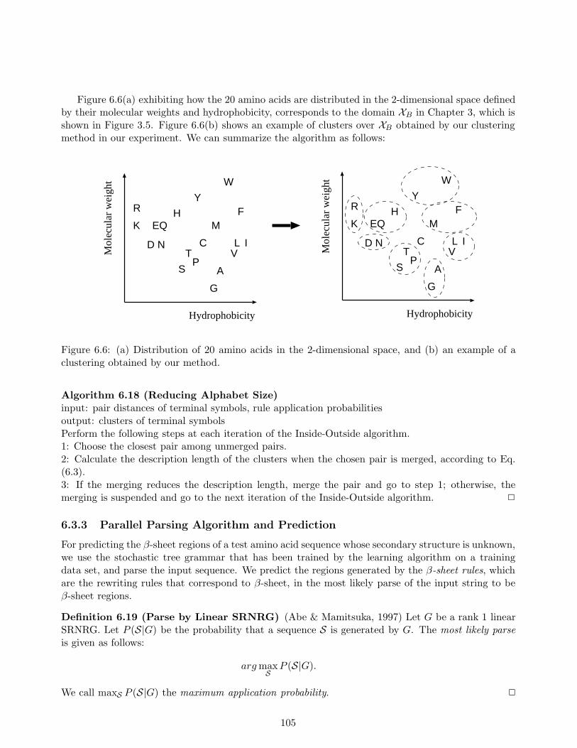
Figure 6.6(a) exhibiting how the 20 amino acids are distributed in the 2-dimensional space definedby their molecular weights and hydrophobicity, corresponds to the domain XB in Chapter 3, which isshown in Figure 3.5. Figure 6.6(b) shows an example of clusters over XB obtained by our clusteringmethod in our experiment. We can summarize the algorithm as follows:

Hydrophobicity

Mol

ecul

ar w

eigh

t

C

R

K EQ

D N

H

Y

W

T

SP

MF

ILV

A

G

HydrophobicityM

olec

ular

wei

ght

C

R

K EQ

D N

H

Y

W

T

SP

MF

ILV

A

G

Figure 6.6: (a) Distribution of 20 amino acids in the 2-dimensional space, and (b) an example of aclustering obtained by our method.

Algorithm 6.18 (Reducing Alphabet Size)input: pair distances of terminal symbols, rule application probabilitiesoutput: clusters of terminal symbolsPerform the following steps at each iteration of the Inside-Outside algorithm.1: Choose the closest pair among unmerged pairs.2: Calculate the description length of the clusters when the chosen pair is merged, according to Eq.(6.3).3: If the merging reduces the description length, merge the pair and go to step 1; otherwise, themerging is suspended and go to the next iteration of the Inside-Outside algorithm. 2

6.3.3 Parallel Parsing Algorithm and Prediction

For predicting the β-sheet regions of a test amino acid sequence whose secondary structure is unknown,we use the stochastic tree grammar that has been trained by the learning algorithm on a trainingdata set, and parse the input sequence. We predict the regions generated by the β-sheet rules, whichare the rewriting rules that correspond to β-sheet, in the most likely parse of the input string to beβ-sheet regions.

Definition 6.19 (Parse by Linear SRNRG) (Abe & Mamitsuka, 1997) Let G be a rank 1 linearSRNRG. Let P (S|G) be the probability that a sequence S is generated by G. The most likely parseis given as follows:

arg maxS

P (S|G).

We call maxS P (S|G) the maximum application probability. 2

105

The parsing algorithm can be generally easily obtained by replacing ‘∑

’ by ‘max’ in the outsidealgorithm (Algorithm 6.11), and retaining the most likely sub-parse at any intermediate step.

As we noted in Section 6.1, we parallelized our parsing algorithm to run on a 32-processor CM-5.In parallelizing this algorithm, we isolated the data dependency by introducing as the outmost loopparameter, d (d = (j − i) + (l − k) in the rank 1 case), which stands for the total length of all thesubstrings that are outside those designated by the current indices. That is, we replace the first fourFor loops in the algorithm for calculating the outside probabilities with those shown below.

For d := n to 0For i := 0 to n − dFor j := i + d to iFor l := n to i + d

This way, the computation of all table entries for a given d could in principle be performed in parallel.Here, in order to reduce the memory requirement of our parsing algorithm, we further placed the

following constraints on the grammars.

1. The grammars are designed so that the applications (i.e. derivation) of rewriting rules alwaystake place in the following order.

Non-β-sheet rules ⇒ β-sheet rules ⇒ Non-β-sheet rules

2. The rule application probabilities of all the non-β-sheet rules are set identically, and the symbolgeneration probabilities in these rewriting rules are fixed.

With the above constraints placed on the grammars, it is no longer necessary to store the partialprobabilities for the applications of non-β-sheet rules, since their contribution to the likelihood of theinput sequence depends only on the length of the non-β-sheet regions in the final analysis, since theirrule application probabilities are all identical.

This enables us not only to save a great deal of run-time memory, but also to significantly cutdown on the computation time as it is no longer necessary to communicate these partial probabilityvalues between the parallel processors. Specifically, with the above constraints the parsing algorithmcan simply search for those four positions (i, j, k, l) which assign the maximum application probabilityto the β-sheet rules, given that their rewriting begins at those positions.

At the cost of sacrificing the generality of the parsing algorithm, this makes it possible to handlea good part of the sequences existing in actual databases of length up to 200 or more in realisticcomputation time.

Let T be the maximum number of processors. For a given test sequence of length n, within thefour loops given above, we allocate to each processor t the computation for all i ∈ I(t), where I(t) isa block of consecutive values of i of size bn/T c or dn/T e. Now, for any given test sequence σ, andfor each processor t, let Lσ[t] be the maximum application probability for β-sheet rules calculated atthe t-th processor. The algorithm computes in parallel Lσ[t] for each processor t, which is to be themaximum of all Lσ[i, j, k, l], which are the application probabilities for β-sheet rules at i, j, k, l for alli ∈ I(t). The details of the algorithm are now exhibited below:

Algorithm 6.20 (Parallel Parsing Algorithm for Linear SRNRG)input: a sequence σ of length n and a rank 1 linear SRNRG Goutput: Pos(tmax), which are the four positions that give the maximum application probability forβ-sheet rules

106

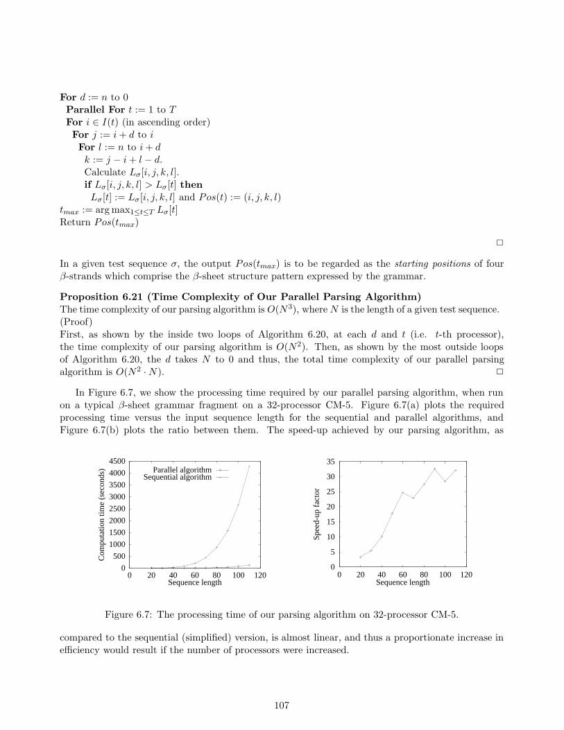
For d := n to 0Parallel For t := 1 to TFor i ∈ I(t) (in ascending order)For j := i + d to iFor l := n to i + dk := j − i + l − d.Calculate Lσ[i, j, k, l].if Lσ[i, j, k, l] > Lσ[t] thenLσ[t] := Lσ[i, j, k, l] and Pos(t) := (i, j, k, l)

tmax := arg max1≤t≤T Lσ[t]Return Pos(tmax)

2

In a given test sequence σ, the output Pos(tmax) is to be regarded as the starting positions of fourβ-strands which comprise the β-sheet structure pattern expressed by the grammar.

Proposition 6.21 (Time Complexity of Our Parallel Parsing Algorithm)The time complexity of our parsing algorithm is O(N3), where N is the length of a given test sequence.(Proof)First, as shown by the inside two loops of Algorithm 6.20, at each d and t (i.e. t-th processor),the time complexity of our parsing algorithm is O(N2). Then, as shown by the most outside loopsof Algorithm 6.20, the d takes N to 0 and thus, the total time complexity of our parallel parsingalgorithm is O(N2 · N). 2

In Figure 6.7, we show the processing time required by our parallel parsing algorithm, when runon a typical β-sheet grammar fragment on a 32-processor CM-5. Figure 6.7(a) plots the requiredprocessing time versus the input sequence length for the sequential and parallel algorithms, andFigure 6.7(b) plots the ratio between them. The speed-up achieved by our parsing algorithm, as

0

500

1000

1500

2000

2500

3000

3500

4000

4500

0 20 40 60 80 100 120

Com

puta

tion

time

(sec

onds

)

Sequence length

Parallel algorithmSequential algorithm

0

5

10

15

20

25

30

35

0 20 40 60 80 100 120

Spee

d-up

fac

tor

Sequence length

Figure 6.7: The processing time of our parsing algorithm on 32-processor CM-5.

compared to the sequential (simplified) version, is almost linear, and thus a proportionate increase inefficiency would result if the number of processors were increased.

107

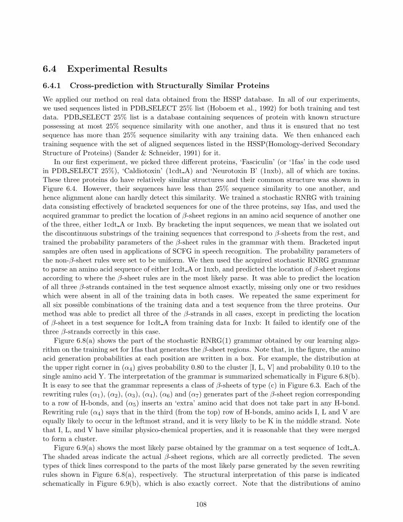
6.4 Experimental Results

6.4.1 Cross-prediction with Structurally Similar Proteins

We applied our method on real data obtained from the HSSP database. In all of our experiments,we used sequences listed in PDB SELECT 25% list (Hoboem et al., 1992) for both training and testdata. PDB SELECT 25% list is a database containing sequences of protein with known structurepossessing at most 25% sequence similarity with one another, and thus it is ensured that no testsequence has more than 25% sequence similarity with any training data. We then enhanced eachtraining sequence with the set of aligned sequences listed in the HSSP(Homology-derived SecondaryStructure of Proteins) (Sander & Schneider, 1991) for it.

In our first experiment, we picked three different proteins, ‘Fasciculin’ (or ‘1fas’ in the code usedin PDB SELECT 25%), ‘Caldiotoxin’ (1cdt A) and ‘Neurotoxin B’ (1nxb), all of which are toxins.These three proteins do have relatively similar structures and their common structure was shown inFigure 6.4. However, their sequences have less than 25% sequence similarity to one another, andhence alignment alone can hardly detect this similarity. We trained a stochastic RNRG with trainingdata consisting effectively of bracketed sequences for one of the three proteins, say 1fas, and used theacquired grammar to predict the location of β-sheet regions in an amino acid sequence of another oneof the three, either 1cdt A or 1nxb. By bracketing the input sequences, we mean that we isolated outthe discontinuous substrings of the training sequences that correspond to β-sheets from the rest, andtrained the probability parameters of the β-sheet rules in the grammar with them. Bracketed inputsamples are often used in applications of SCFG in speech recognition. The probability parameters ofthe non-β-sheet rules were set to be uniform. We then used the acquired stochastic RNRG grammarto parse an amino acid sequence of either 1cdt A or 1nxb, and predicted the location of β-sheet regionsaccording to where the β-sheet rules are in the most likely parse. It was able to predict the locationof all three β-strands contained in the test sequence almost exactly, missing only one or two residueswhich were absent in all of the training data in both cases. We repeated the same experiment forall six possible combinations of the training data and a test sequence from the three proteins. Ourmethod was able to predict all three of the β-strands in all cases, except in predicting the locationof β-sheet in a test sequence for 1cdt A from training data for 1nxb: It failed to identify one of thethree β-strands correctly in this case.

Figure 6.8(a) shows the part of the stochastic RNRG(1) grammar obtained by our learning algo-rithm on the training set for 1fas that generates the β-sheet regions. Note that, in the figure, the aminoacid generation probabilities at each position are written in a box. For example, the distribution atthe upper right corner in (α4) gives probability 0.80 to the cluster [I, L, V] and probability 0.10 to thesingle amino acid Y. The interpretation of the grammar is summarized schematically in Figure 6.8(b).It is easy to see that the grammar represents a class of β-sheets of type (c) in Figure 6.3. Each of therewriting rules (α1), (α2), (α3), (α4), (α6) and (α7) generates part of the β-sheet region correspondingto a row of H-bonds, and (α5) inserts an ‘extra’ amino acid that does not take part in any H-bond.Rewriting rule (α4) says that in the third (from the top) row of H-bonds, amino acids I, L and V areequally likely to occur in the leftmost strand, and it is very likely to be K in the middle strand. Notethat I, L, and V have similar physico-chemical properties, and it is reasonable that they were mergedto form a cluster.

Figure 6.9(a) shows the most likely parse obtained by the grammar on a test sequence of 1cdt A.The shaded areas indicate the actual β-sheet regions, which are all correctly predicted. The seventypes of thick lines correspond to the parts of the most likely parse generated by the seven rewritingrules shown in Figure 6.8(a), respectively. The structural interpretation of this parse is indicatedschematically in Figure 6.9(b), which is also exactly correct. Note that the distributions of amino

108

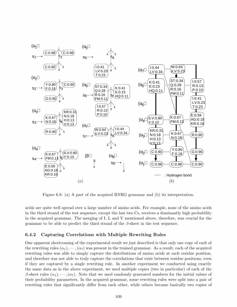
s st

C:0.98 C:0.98

C:0.90

1 2

t(α )1

st

Y:0.80F:0.18

C:0.90

G:0.90

3

t(α )2

st

K:0.67N:0.18

KR:0.31N:0.18H:0.13V:0.13

R:0.90

4

t(α )3

st

K:0.67FM:0.13

ILV:0.80Y:0.10

E:0.59AG:0.18KR:0.16

5

t(α )4

st

I:0.41LV:0.23T:0.23

6

t(α )5

st

ST:0.34Q:0.28R:0.16FM:0.11

K:0.41E:0.23HQ:0.11

I:0.57R:0.13P:0.10

7

t(α )6

st

W:0.64ILV:0.23

I:0.44LV:0.34

8

t(α )7

s2

s3

s4

s5

s6

s7

(β)s

(α )8

s8 t

λ

λ

λ

λ λ

λ λ

λ

λ

λλ

#

#

#

#

#

#

#

#

C:0.98 C:0.98 C:0.90

(α )3

(α )5

(α )6

W:0.64ILV:0.23(α )7

(α )4

(α )2

(α )1

I:0.44LV:0.34

K:0.41E:0.23HQ:0.11

ILV:0.80Y:0.10

KR:0.31N:0.18H:0.13V:0.13

C:0.90

ST:0.34Q:0.28R:0.16FM:0.11

K:0.67FM:0.13

K:0.67N:0.18

Y:0.80F:0.18 G:0.90

R:0.90

E:0.59AG:0.18KR:0.16

I:0.41LV:0.23T:0.23

I:0.57R:0.13P:0.10

: Hydrogen bond

(a) (b)

Figure 6.8: (a) A part of the acquired RNRG grammar and (b) its interpretation.

acids are quite well spread over a large number of amino acids. For example, none of the amino acidsin the third strand of the test sequence, except the last two Cs, receives a dominantly high probabilityin the acquired grammar. The merging of I, L and V mentioned above, therefore, was crucial for thegrammar to be able to predict the third strand of the β-sheet in the test sequence.

6.4.2 Capturing Correlations with Multiple Rewriting Rules

One apparent shortcoming of the experimental result we just described is that only one copy of each ofthe rewriting rules (α1), · · · , (α7) was present in the trained grammar. As a result, each of the acquiredrewriting rules was able to simply capture the distributions of amino acids at each residue position,and therefore was not able to truly capture the correlations that exist between residue positions, evenif they are captured by a single rewriting rule. In another experiment we conducted using exactlythe same data as in the above experiment, we used multiple copies (two in particular) of each of theβ-sheet rules (α1), · · · , (α7). Note that we used randomly generated numbers for the initial values oftheir probability parameters. In the acquired grammar, some rewriting rules were split into a pair ofrewriting rules that significantly differ from each other, while others became basically two copies of

109

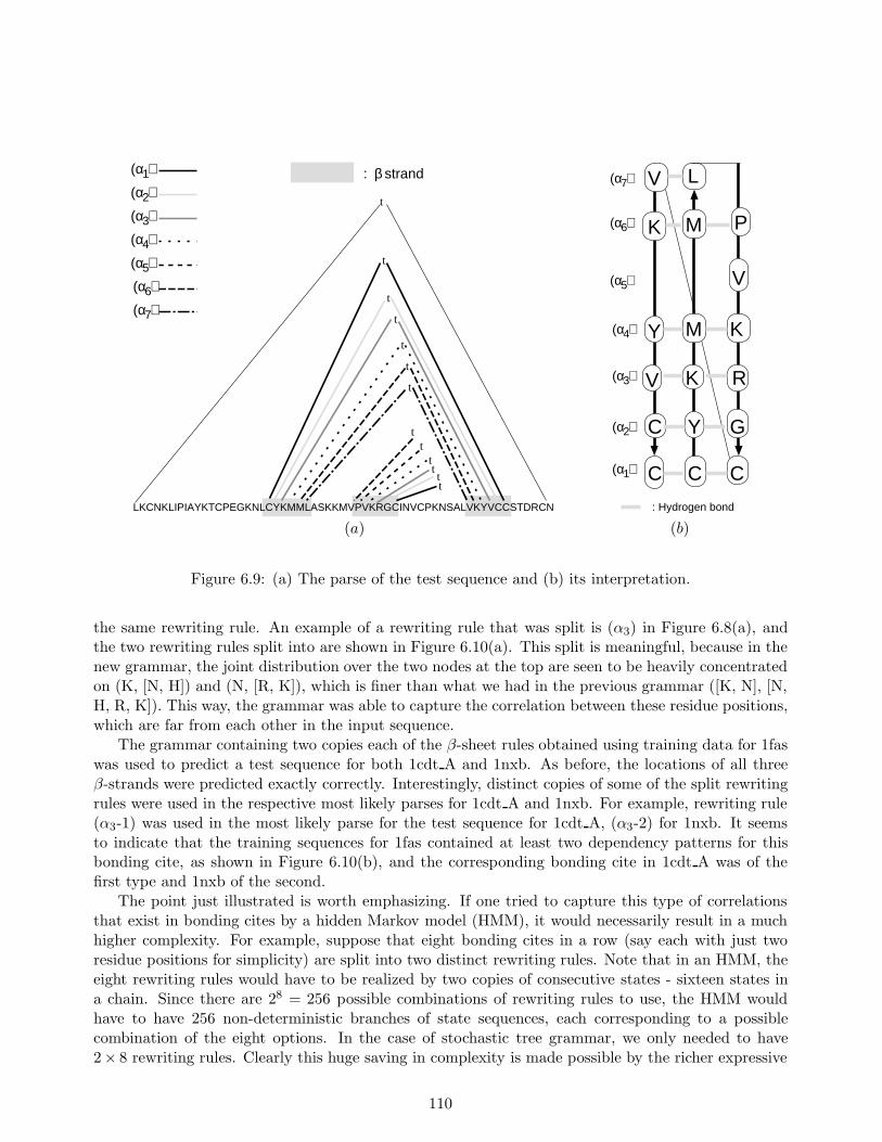
(α )5

(α )3

(α )2

(α )1

(α )4

(α )6

(α )7

LKCNKLIPIAYKTCPEGKNLCYKMMLASKKMVPVKRGCINVCPKNSALVKYVCCSTDRCN

: β strand

t

t

t

t

t

t

tt

tttt

t

C C C

(α )3

(α )5

(α )6

L(α )7

(α )4

(α )2

(α )1

V

K

Y

V

C

M

M

K

Y G

R

K

V

P

: Hydrogen bond

(a) (b)

Figure 6.9: (a) The parse of the test sequence and (b) its interpretation.

the same rewriting rule. An example of a rewriting rule that was split is (α3) in Figure 6.8(a), andthe two rewriting rules split into are shown in Figure 6.10(a). This split is meaningful, because in thenew grammar, the joint distribution over the two nodes at the top are seen to be heavily concentratedon (K, [N, H]) and (N, [R, K]), which is finer than what we had in the previous grammar ([K, N], [N,H, R, K]). This way, the grammar was able to capture the correlation between these residue positions,which are far from each other in the input sequence.

The grammar containing two copies each of the β-sheet rules obtained using training data for 1faswas used to predict a test sequence for both 1cdt A and 1nxb. As before, the locations of all threeβ-strands were predicted exactly correctly. Interestingly, distinct copies of some of the split rewritingrules were used in the respective most likely parses for 1cdt A and 1nxb. For example, rewriting rule(α3-1) was used in the most likely parse for the test sequence for 1cdt A, (α3-2) for 1nxb. It seemsto indicate that the training sequences for 1fas contained at least two dependency patterns for thisbonding cite, as shown in Figure 6.10(b), and the corresponding bonding cite in 1cdt A was of thefirst type and 1nxb of the second.

The point just illustrated is worth emphasizing. If one tried to capture this type of correlationsthat exist in bonding cites by a hidden Markov model (HMM), it would necessarily result in a muchhigher complexity. For example, suppose that eight bonding cites in a row (say each with just tworesidue positions for simplicity) are split into two distinct rewriting rules. Note that in an HMM, theeight rewriting rules would have to be realized by two copies of consecutive states - sixteen states ina chain. Since there are 28 = 256 possible combinations of rewriting rules to use, the HMM wouldhave to have 256 non-deterministic branches of state sequences, each corresponding to a possiblecombination of the eight options. In the case of stochastic tree grammar, we only needed to have2× 8 rewriting rules. Clearly this huge saving in complexity is made possible by the richer expressive

110

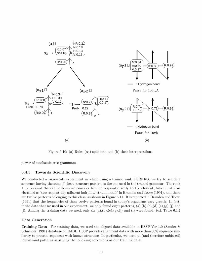
st

K:0.67N:0.18

KR:0.31N:0.18H:0.13V:0.13

R:0.90

4

t(α )3

s st

K:0.88

N:0.34H:0.30V:0.17

R:0.99

3 4

t

(α )3

s st

N:0.71R:0.71K:0.17

R:0.99

3 4

t

(α )3

Prob. : 0.78 Prob. : 0.22

-1 -2

s3

λ

λ λ

#

# #

(α )3N:0.34H:0.30V:0.17

K:0.88 R:0.99

: Hydrogen bond

-1

Parse for 1cdt A

(α )3R:0.71K:0.17 N:0.71 R:0.99

: Hydrogen bond

-2

Parse for 1nxb

(a) (b)

Figure 6.10: (a) Rules (α3) split into and (b) their interpretations.

power of stochastic tree grammars.

6.4.3 Towards Scientific Discovery

We conducted a large-scale experiment in which using a trained rank 1 SRNRG, we try to search asequence having the same β-sheet structure pattern as the one used in the trained grammar. The rank1 four-strand β-sheet patterns we consider here correspond exactly to the class of β-sheet patternsclassified as ‘two sequentially adjacent hairpin β-strand motifs’ in Branden and Tooze (1991), and thereare twelve patterns belonging to this class, as shown in Figure 6.11. It is reported in Branden and Tooze(1991) that the frequencies of these twelve patterns found in today’s organisms vary greatly. In fact,in the data that we used in our experiment, we only found eight patterns, (a),(b),(c),(d),(e),(g),(j) and(l). Among the training data we used, only six (a),(b),(c),(g),(j) and (l) were found. (c.f. Table 6.1.)

Data Generation

Training Data For training data, we used the aligned data available in HSSP Ver 1.0 (Sander &Schneider, 1991) database of EMBL. HSSP provides alignment data with more than 30% sequence sim-ilarity to protein sequences with known structure. In particular, we used all (and therefore unbiased)four-strand patterns satisfying the following conditions as our training data.

111

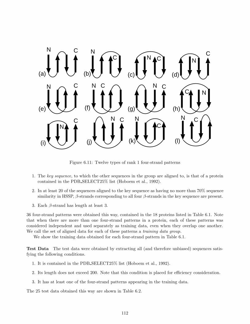
N

N

N

N

N

N N N

N

N N

N

C

C

C

C

CC

C

C

C

CC

C

(a)

(e)

(i) (j) (k) (l)

(h)

(d)(c)(b)

(f) (g)

Figure 6.11: Twelve types of rank 1 four-strand patterns

1. The key sequence, to which the other sequences in the group are aligned to, is that of a proteincontained in the PDB SELECT25% list (Hoboem et al., 1992).

2. In at least 20 of the sequences aligned to the key sequence as having no more than 70% sequencesimilarity in HSSP, β-strands corresponding to all four β-strands in the key sequence are present.

3. Each β-strand has length at least 3.

36 four-strand patterns were obtained this way, contained in the 18 proteins listed in Table 6.1. Notethat when there are more than one four-strand patterns in a protein, each of these patterns wasconsidered independent and used separately as training data, even when they overlap one another.We call the set of aligned data for each of these patterns a training data group.

We show the training data obtained for each four-strand pattern in Table 6.1.

Test Data The test data were obtained by extracting all (and therefore unbiased) sequences satis-fying the following conditions.

1. It is contained in the PDB SELECT25% list (Hoboem et al., 1992).

2. Its length does not exceed 200. Note that this condition is placed for efficiency consideration.

3. It has at least one of the four-strand patterns appearing in the training data.

The 25 test data obtained this way are shown in Table 6.2.

112

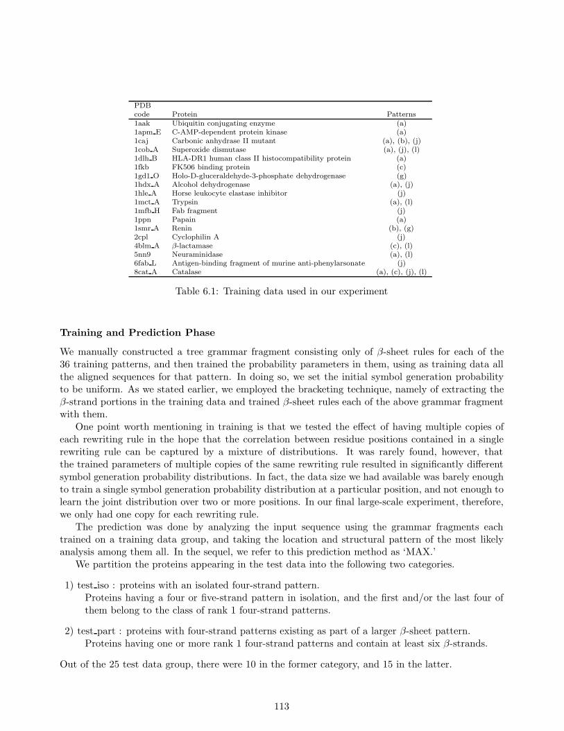
PDBcode Protein Patterns1aak Ubiquitin conjugating enzyme (a)1apm E C-AMP-dependent protein kinase (a)1caj Carbonic anhydrase II mutant (a), (b), (j)1cob A Superoxide dismutase (a), (j), (l)1dlh B HLA-DR1 human class II histocompatibility protein (a)1fkb FK506 binding protein (c)1gd1 O Holo-D-gluceraldehyde-3-phosphate dehydrogenase (g)1hdx A Alcohol dehydrogenase (a), (j)1hle A Horse leukocyte elastase inhibitor (j)1mct A Trypsin (a), (l)1mfb H Fab fragment (j)1ppn Papain (a)1smr A Renin (b), (g)2cpl Cyclophilin A (j)4blm A β-lactamase (c), (l)5nn9 Neuraminidase (a), (l)6fab L Antigen-binding fragment of murine anti-phenylarsonate (j)8cat A Catalase (a), (c), (j), (l)

Table 6.1: Training data used in our experiment

Training and Prediction Phase

We manually constructed a tree grammar fragment consisting only of β-sheet rules for each of the36 training patterns, and then trained the probability parameters in them, using as training data allthe aligned sequences for that pattern. In doing so, we set the initial symbol generation probabilityto be uniform. As we stated earlier, we employed the bracketing technique, namely of extracting theβ-strand portions in the training data and trained β-sheet rules each of the above grammar fragmentwith them.

One point worth mentioning in training is that we tested the effect of having multiple copies ofeach rewriting rule in the hope that the correlation between residue positions contained in a singlerewriting rule can be captured by a mixture of distributions. It was rarely found, however, thatthe trained parameters of multiple copies of the same rewriting rule resulted in significantly differentsymbol generation probability distributions. In fact, the data size we had available was barely enoughto train a single symbol generation probability distribution at a particular position, and not enough tolearn the joint distribution over two or more positions. In our final large-scale experiment, therefore,we only had one copy for each rewriting rule.

The prediction was done by analyzing the input sequence using the grammar fragments eachtrained on a training data group, and taking the location and structural pattern of the most likelyanalysis among them all. In the sequel, we refer to this prediction method as ‘MAX.’

We partition the proteins appearing in the test data into the following two categories.

1) test iso : proteins with an isolated four-strand pattern.Proteins having a four or five-strand pattern in isolation, and the first and/or the last four ofthem belong to the class of rank 1 four-strand patterns.

2) test part : proteins with four-strand patterns existing as part of a larger β-sheet pattern.Proteins having one or more rank 1 four-strand patterns and contain at least six β-strands.

Out of the 25 test data group, there were 10 in the former category, and 15 in the latter.

113

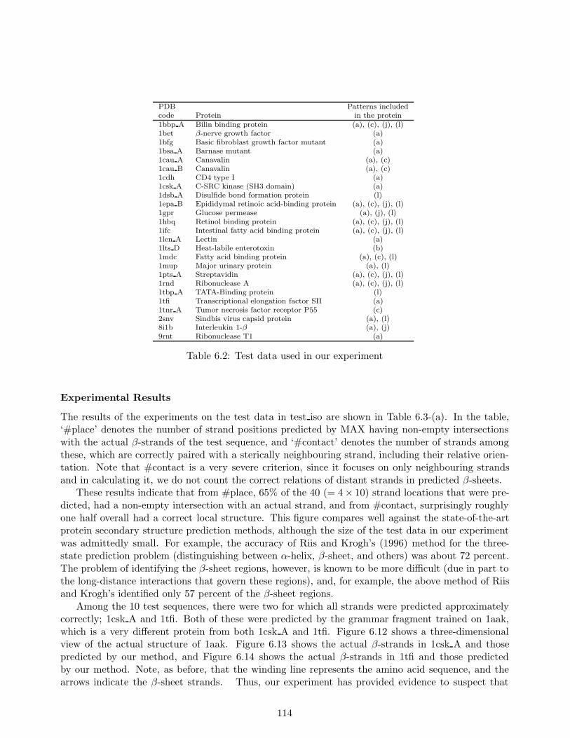
PDB Patterns includedcode Protein in the protein1bbp A Bilin binding protein (a), (c), (j), (l)1bet β-nerve growth factor (a)1bfg Basic fibroblast growth factor mutant (a)1bsa A Barnase mutant (a)1cau A Canavalin (a), (c)1cau B Canavalin (a), (c)1cdh CD4 type I (a)1csk A C-SRC kinase (SH3 domain) (a)1dsb A Disulfide bond formation protein (l)1epa B Epididymal retinoic acid-binding protein (a), (c), (j), (l)1gpr Glucose permease (a), (j), (l)1hbq Retinol binding protein (a), (c), (j), (l)1ifc Intestinal fatty acid binding protein (a), (c), (j), (l)1len A Lectin (a)1lts D Heat-labile enterotoxin (b)1mdc Fatty acid binding protein (a), (c), (l)1mup Major urinary protein (a), (l)1pts A Streptavidin (a), (c), (j), (l)1rnd Ribonuclease A (a), (c), (j), (l)1tbp A TATA-Binding protein (l)1tfi Transcriptional elongation factor SII (a)1tnr A Tumor necrosis factor receptor P55 (c)2snv Sindbis virus capsid protein (a), (l)8i1b Interleukin 1-β (a), (j)9rnt Ribonuclease T1 (a)

Table 6.2: Test data used in our experiment

Experimental Results

The results of the experiments on the test data in test iso are shown in Table 6.3-(a). In the table,‘#place’ denotes the number of strand positions predicted by MAX having non-empty intersectionswith the actual β-strands of the test sequence, and ‘#contact’ denotes the number of strands amongthese, which are correctly paired with a sterically neighbouring strand, including their relative orien-tation. Note that #contact is a very severe criterion, since it focuses on only neighbouring strandsand in calculating it, we do not count the correct relations of distant strands in predicted β-sheets.

These results indicate that from #place, 65% of the 40 (= 4× 10) strand locations that were pre-dicted, had a non-empty intersection with an actual strand, and from #contact, surprisingly roughlyone half overall had a correct local structure. This figure compares well against the state-of-the-artprotein secondary structure prediction methods, although the size of the test data in our experimentwas admittedly small. For example, the accuracy of Riis and Krogh’s (1996) method for the three-state prediction problem (distinguishing between α-helix, β-sheet, and others) was about 72 percent.The problem of identifying the β-sheet regions, however, is known to be more difficult (due in part tothe long-distance interactions that govern these regions), and, for example, the above method of Riisand Krogh’s identified only 57 percent of the β-sheet regions.

Among the 10 test sequences, there were two for which all strands were predicted approximatelycorrectly; 1csk A and 1tfi. Both of these were predicted by the grammar fragment trained on 1aak,which is a very different protein from both 1csk A and 1tfi. Figure 6.12 shows a three-dimensionalview of the actual structure of 1aak. Figure 6.13 shows the actual β-strands in 1csk A and thosepredicted by our method, and Figure 6.14 shows the actual β-strands in 1tfi and those predictedby our method. Note, as before, that the winding line represents the amino acid sequence, and thearrows indicate the β-sheet strands. Thus, our experiment has provided evidence to suspect that

114

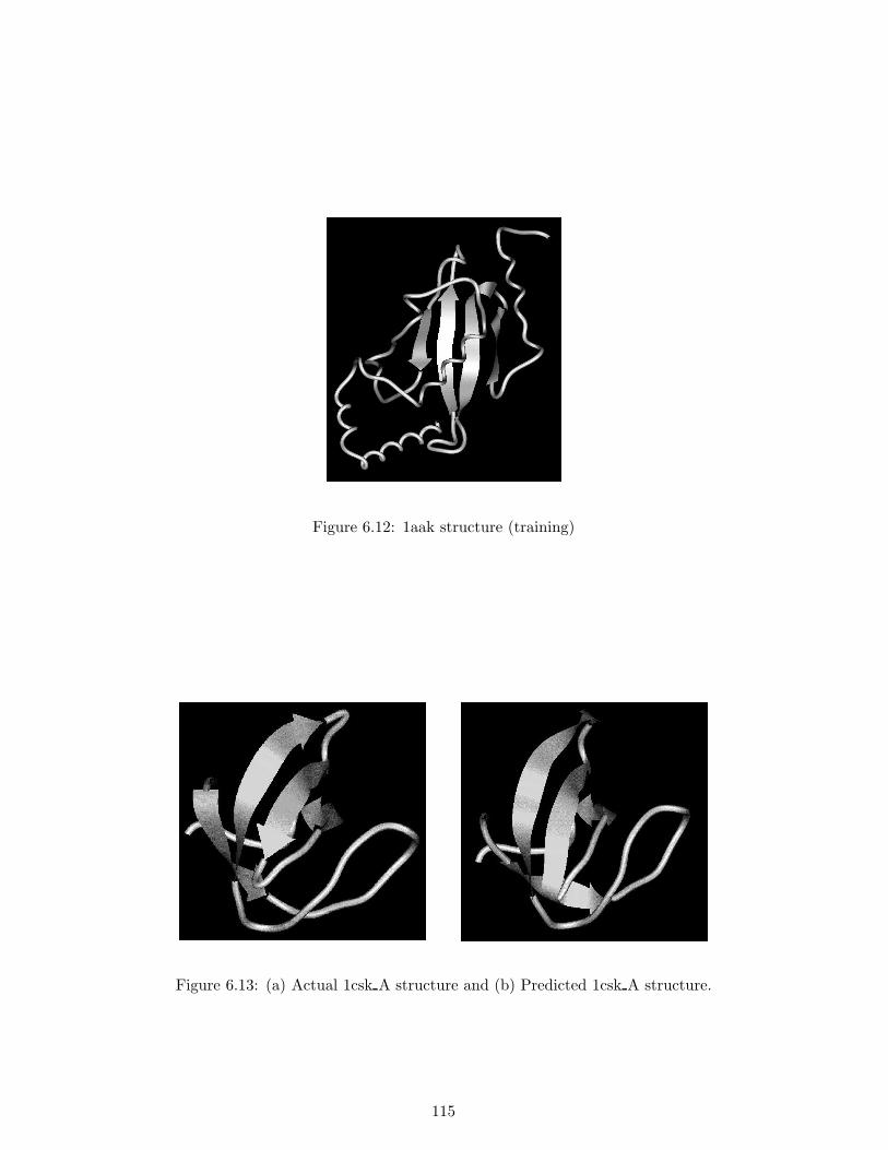
Figure 6.12: 1aak structure (training)

Figure 6.13: (a) Actual 1csk A structure and (b) Predicted 1csk A structure.

115

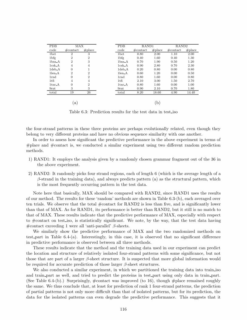
PDB MAXcode #contact #place1bet 2 31bfg 2 21bsa A 2 31csk A 4 41dsb A 0 11len A 2 21rnd 0 21tfi 4 41tnr A 0 29rnt 3 3total 19 26

PDB RAND1 RAND2code #contact #place #contact #place1bet 0.80 2.00 1.10 2.001bfg 0.40 1.60 0.40 1.301bsa A 0.70 1.90 0.50 1.201csk A 0.90 2.80 0.70 2.301dsb A 0.20 0.80 0.00 0.801len A 0.60 1.20 0.00 0.501rnd 0.80 1.60 0.00 0.801tfi 2.10 3.00 1.50 2.701tnr A 0.80 1.60 0.00 1.009rnt 0.90 2.10 0.70 1.80total 8.20 18.60 4.90 14.40

(a) (b)

Table 6.3: Prediction results for the test data in test iso

the four-strand patterns in these three proteins are perhaps evolutionally related, even though theybelong to very different proteins and have no obvious sequence similarity with one another.

In order to assess how significant the predictive performance in the above experiment in terms of#place and #contact is, we conducted a similar experiment using two different random predictionmethods.

1) RAND1: It employs the analysis given by a randomly chosen grammar fragment out of the 36 inthe above experiment.

2) RAND2: It randomly picks four strand regions, each of length 6 (which is the average length of aβ-strand in the training data), and always predicts pattern (a) as the structural pattern, whichis the most frequently occurring pattern in the test data.

Note here that basically, MAX should be compared with RAND2, since RAND1 uses the resultsof our method. The results for these ‘random’ methods are shown in Table 6.3-(b), each averaged overten trials. We observe that the total #contact for RAND2 is less than five, and is significantly lowerthan that of MAX. As for RAND1, its performance is better than RAND2, but it still is no match tothat of MAX. These results indicate that the predictive performance of MAX, especially with respectto #contact on test iso, is statistically significant. We note, by the way, that the test data having#contact exceeding 1 were all ‘anti-parallel’ β-sheets.

We similarly show the predictive performance of MAX and the two randomized methods ontest part in Table 6.4-(a). Interestingly, in this case, it is observed that no significant differencein predictive performance is observed between all three methods.

These results indicate that the method and the training data used in our experiment can predictthe location and structure of relatively isolated four-strand patterns with some significance, but notthose that are part of a larger β-sheet structure. It is suspected that more global information wouldbe required for accurate prediction of those larger β-sheet structures.

We also conducted a similar experiment, in which we partitioned the training data into train isoand train part as well, and tried to predict the proteins in test part using only data in train part.(See Table 6.4-(b).) Surprisingly, #contact was improved (to 16), though #place remained roughlythe same. We thus conclude that, at least for prediction of rank 1 four-strand patterns, the predictionof partial patterns is not only more difficult than that of isolated patterns, but for its prediction, thedata for the isolated patterns can even degrade the predictive performance. This suggests that it

116

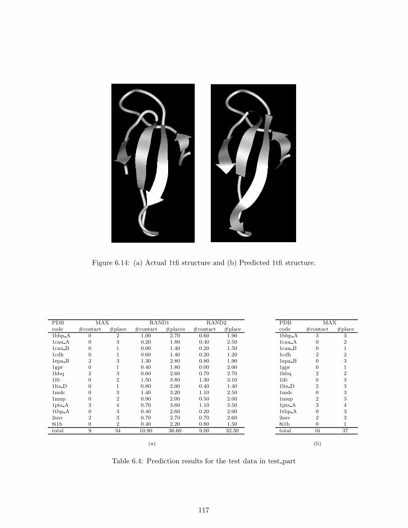
Figure 6.14: (a) Actual 1tfi structure and (b) Predicted 1tfi structure.

PDB MAX RAND1 RAND2code #contact #place #contact #places #contact #place1bbp A 0 2 1.00 2.70 0.60 1.901cau A 0 3 0.20 1.80 0.40 2.501cau B 0 1 0.00 1.40 0.20 1.501cdh 0 1 0.60 1.40 0.20 1.201epa B 2 3 1.30 2.80 0.80 1.901gpr 0 1 0.40 1.80 0.00 2.001hbq 2 3 0.60 2.60 0.70 2.701ifc 0 2 1.50 3.80 1.30 3.101lts D 0 1 0.80 2.00 0.40 1.401mdc 0 3 1.40 3.20 1.10 2.501mup 0 2 0.90 2.00 0.50 2.001pts A 3 4 0.70 3.60 1.10 3.501tbp A 0 3 0.40 2.60 0.20 2.002snv 2 3 0.70 2.70 0.70 2.608i1b 0 2 0.40 2.20 0.80 1.50total 9 34 10.90 36.60 9.00 32.30

PDB MAXcode #contact #place1bbp A 3 31cau A 0 21cau B 0 11cdh 2 21epa B 0 31gpr 0 11hbq 2 21ifc 0 31lts D 2 31mdc 0 31mup 2 31pts A 3 41tbp A 0 32snv 2 38i1b 0 1total 16 37

(a) (b)

Table 6.4: Prediction results for the test data in test part

117

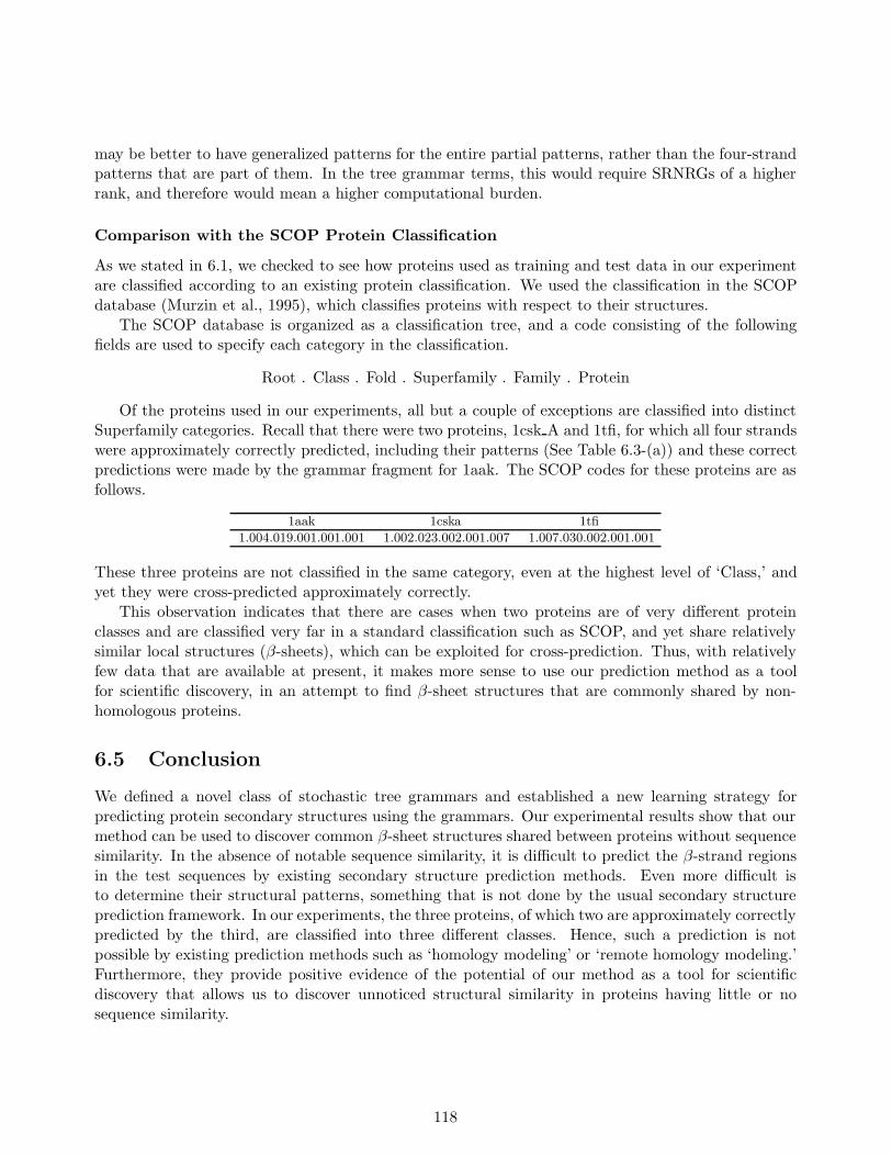
may be better to have generalized patterns for the entire partial patterns, rather than the four-strandpatterns that are part of them. In the tree grammar terms, this would require SRNRGs of a higherrank, and therefore would mean a higher computational burden.

Comparison with the SCOP Protein Classification

As we stated in 6.1, we checked to see how proteins used as training and test data in our experimentare classified according to an existing protein classification. We used the classification in the SCOPdatabase (Murzin et al., 1995), which classifies proteins with respect to their structures.

The SCOP database is organized as a classification tree, and a code consisting of the followingfields are used to specify each category in the classification.

Root . Class . Fold . Superfamily . Family . Protein

Of the proteins used in our experiments, all but a couple of exceptions are classified into distinctSuperfamily categories. Recall that there were two proteins, 1csk A and 1tfi, for which all four strandswere approximately correctly predicted, including their patterns (See Table 6.3-(a)) and these correctpredictions were made by the grammar fragment for 1aak. The SCOP codes for these proteins are asfollows.

1aak 1cska 1tfi

1.004.019.001.001.001 1.002.023.002.001.007 1.007.030.002.001.001

These three proteins are not classified in the same category, even at the highest level of ‘Class,’ andyet they were cross-predicted approximately correctly.

This observation indicates that there are cases when two proteins are of very different proteinclasses and are classified very far in a standard classification such as SCOP, and yet share relativelysimilar local structures (β-sheets), which can be exploited for cross-prediction. Thus, with relativelyfew data that are available at present, it makes more sense to use our prediction method as a toolfor scientific discovery, in an attempt to find β-sheet structures that are commonly shared by non-homologous proteins.

6.5 Conclusion

We defined a novel class of stochastic tree grammars and established a new learning strategy forpredicting protein secondary structures using the grammars. Our experimental results show that ourmethod can be used to discover common β-sheet structures shared between proteins without sequencesimilarity. In the absence of notable sequence similarity, it is difficult to predict the β-strand regionsin the test sequences by existing secondary structure prediction methods. Even more difficult isto determine their structural patterns, something that is not done by the usual secondary structureprediction framework. In our experiments, the three proteins, of which two are approximately correctlypredicted by the third, are classified into three different classes. Hence, such a prediction is notpossible by existing prediction methods such as ‘homology modeling’ or ‘remote homology modeling.’Furthermore, they provide positive evidence of the potential of our method as a tool for scientificdiscovery that allows us to discover unnoticed structural similarity in proteins having little or nosequence similarity.

118

Chapter 7

Concluding Remarks and FuturePerspective

7.1 Summary

We defined four stochastic knowledge representations, i.e. a stochastic rule with finite partitioning, aprobabilistic network with finite partitionings, a hidden Markov model and a stochastic ranked noderewriting grammar, and established new learning algorithms for the four knowledge representations.The learning algorithms we established are the following three:1) methods based on the Minimum Description Length (MDL) criterion,2) a gradient method for minimizing a type of error-distance function, and3) a method based on the Expectation-Maximization (EM) algorithm.

The methods based on the MDL criterion were proposed to estimate the number of cells in astochastic rule with finite partitioning in Chapter 3, to estimate the structure of a probabilisticnetwork with finite partitionings in Chapter 4, and to cluster an alphabet in Chapter 6. Thesealgorithms have a significant characteristic that allows us to estimate not only probability parametersin a given stochastic model but also the stochastic model itself. In other words, a number of featureshidden in given training examples can be automatically found by this type of model estimation.

The gradient method for minimizing a type of error-distance function was proposed to estimateprobability parameters of hidden Markov models (HMMs) in Chapter 5. This algorithm allows usto perform supervised learning, which has never been done for HMMs, and improve the predictiveperformance of HMMs. Similar algorithms were applied to train neural networks, which were used tocompare the performance of neural network methods with that of our methods, in Chapters 3, 4 and5.

The learning algorithm based on the EM algorithm was proposed to estimate probability param-eters of stochastic ranked node rewriting grammars in Chapter 6. No learning algorithms had everpreviously been proposed for the grammars, and the algorithm helps make it possible to efficientlyestimate the parameters of such complicated grammars. A similar learning algorithm for HMMs,called the Baum-Welch, was applied in Chapter 5 for purposes of comparison with our supervisedlearning algorithm for HMMs.

We evaluated these methods by computer experiments, using actual biological sequences. Ex-perimental results showed that all of the knowledge representations defined and the new learningalgorithms established greatly contribute to the crucial problems of computational molecular biology.In Chapter 3, for the problem of predicting α-helices, our method achieved a prediction accuracy ofnearly the same level as that of the best method at that time. In Chapter 4, from a number of se-

119

quences of a particular motif, our method found a number of features hidden in the motif. In Chapter5, our supervised learning method for HMMs improves the predictive performance of the conventionalalgorithm for HMMs, and for the problem of predicting peptides binding to an MHC molecule, ourmethod achieves a predictive performance which exceeds those of the existing methods applied tothe problem. As described in Chapter 6, our method was actually able to capture the long distancedependency in β-sheet regions in a way that had not been possible using any earlier method.

7.2 Future Directions

We here describe possible future work to improve our four learning strategies.

Predicting α-helices with Stochastic Rule Learning

1) Correlations among residues.In the SR method, we assumed for simplicity’s sake that all residues in an α-helix region of atraining protein are probabilistically independent (see Eq. (3.1)). However, it is rather morenatural to suppose that there may exist some mutual correlation among the residues which affecttheir secondary structures. In fact, there are several methods that consider a mutual correlationamong residues in an α-helix (c.f. Gibrat, Garnier, & Robson, 1987), and the neural networklearning methods themselves are correlation-based methods. Considering residue interactions inthe SR method will improve its predictive performance. One possible way for this improvementis the probabilistic network with finite partitionings given in Chapter 4, in which inter-residuerelations are automatically obtained by our learning algorithm. This network, however, has notbeen applied to predicting α-helices. This is an important topic which remains for future study.

2) Considering for long-range interactionsOur experiments in Chapter 3 showed that the average prediction accuracy (81%) and the α-helixcontent rate for the test proteins only slightly differed from those for the training proteins (84%prediction accuracy). This suggests that for the α-helix prediction methods based on the localproperties in the primary structure, we have come close to the limit of prediction accuracy.Considering long-range interactions in the primary structure in addition to its local properties isindispensable to improve the current predictive performance, and is a challenging future issue.We note that the stochastic ranked node rewriting grammar proposed in Chapter 6 is one methodfor capturing such long-distance dependencies. The challenge is to apply such a grammar, orpropose a new method, which can capture such long-distance dependencies to further improvethe predictive performance.

Learning Probabilistic Networks

Supervised learning for probabilistic networkIn Chapter 4, we train a probabilistic network with finite partitionings from given positiveexamples. In short, we perform unsupervised learning for the network. Thus, in Chapter 4, theaverage prediction accuracy of our networks is slightly lower than that of neural networks trainedby a supervised learning method. This indicates that if we could perform supervised learningto train our network, a higher prediction accuracy might be obtained. Supervised learning forthe probabilistic network with finite partitionings is a possible future project.

120

Supervised Learning of Hidden Markov Models

Faster learning algorithmIn our supervised learning algorithm, the computation time per iteration is on the same order asthat of the Baum-Welch algorithm. However, the number of iterations required in our algorithmuntil the updated parameter values converge is far larger than that of the Baum-Welch. Thus,a possible future work is to propose a faster algorithm for supervised learning of HMMs.

Learning Stochastic Tree Grammars

1) Cutting down on computational requirement.The most important future challenge is to reduce the rather high computational requirement ofour parsing algorithm, which has prohibited us to date from conducting full scale experimentsin which the β-sheet structure of an arbitrary amino acid sequence is predicted.

2) Stochastic grammar with richer expressive power.As is shown in Chapter 6, a linear stochastic ranked node rewriting grammar is suitable forrepresenting the structures of β-sheets, but if we deal with more complicated residue contactsin a protein, we have to consider more general grammars than a linear stochastic ranked noderewriting grammar. Thus, another possible future work related to stochastic tree grammars isto define a more general stochastic grammar which has a richer expressive power than that of alinear stochastic ranked node rewriting grammar, but for which efficient learning and parsing al-gorithms can be proposed. We believe that this type of research direction will greatly contributeto the field of computer science as well as computational molecular biology.

121

Bibliography

Abe, N. (1988). Feasible learnability of formal grammars and the theory of natural language acquision.In Proceedings of the International Conference on Computational Linguistics, pp. 1–6 Budapest,Hungary.

Abe, N., & Mamitsuka, H. (1994). A new method for predicting protein secondary structures basedon stochastic tree grammars. In Proceedings of the 11th International Conference on MachineLearning, pp. 3–11 New Brunswick, NJ. Morgan Kaufmann.

Abe, N., & Mamitsuka, H. (1997). Predicting protein secondary structure using stochastic tree gram-mars. Machine Learning, 29, 275–301.

Abe, N., & Mamitsuka, H. (1998). Query learning strategies using boosting and bagging. In Proceed-ings of the 15th International Conference on Machine Learning, pp. 1–9 Madison, WI. MorganKaufmann.

Altschul, S. F., Boguski, M. S., Gish, W., & Wooton, J. C. (1994). Issues in searching molecularsequence database. Nature Genetics, 6, 119–129.

Anfinsen, C. B. (1973). Principles that govern the folding of protein chains. Science, 181, 223–230.

Asai, K., Hayamizu, S., & Handa, K. (1993). Prediction of protein secondary structure by the hiddenMarkov model. Comput. Applic. Biosci., 9, 141–146.

Bahl, L. R., Brown, P. F., de Souza, P. V., & Mercer, R. L. (1986). Maximum mutual informationestimation of hidden Markov models parameters for speech recognition. In Proceedings IEEEInternational Conference on Acoustics, Speech and Signal Processing, Vol. 1, pp. 49–52.

Bairoch, A., & Apweiler, R. (1996). The SWISS-PROT protein sequence data bank and its newsupplement TrEMBL. Nucl. Acids Res., 24, 21–25.

Bairoch, A., & Apweiler, R. (1999). The SWISS-PROT protein sequence data bank and its supplementTrEMBL in 1999. Nucl. Acids Res., 27 (1), 49–55.

Bairoch, A., P.Bucher, & Hofmann, K. (1996). The PROSITE database, its status in 1996. Nucl.Acids Res., 24, 189–196.

Baldi, P., & Chauvin, Y. (1994a). Hidden Markov models of the G-protein-coupled receptor family.J. Comput. Biol., 1 (4), 311–326.

Baldi, P., & Chauvin, Y. (1994b). Smooth on-line learning algorithms for hidden Markov models.Neural Comp., 6, 307–318.

122

Baldi, P., Chauvin, Y., Hunkapillar, T., & McClure, M. (1994). Hidden Markov models of biologicalprimary sequence information. Proc. Natl. Acad. Sci., 91, 1059–1063.

Barker, W. C., Garavelli, J. S., McGarvey, P. B., Marzec, C. R., Orcutt, B. C., Srinivasarao, G. Y.,Yeh, L-S. L., Ledley, R. S., Mewes, H-W., Pfeiffer, F., Tsugita, A., & Wu, C. (1999). ThePIR-international protein sequence database. Nucl. Acids Res., 27 (1), 39–43.

Barron, A. R., & Cover, T. M. (1991). Minimum complexity density estimation. IEEE Trans. onInformation Theory (IT), IT-37, 1034–1054.

Barton, G. J. (1995). Protein secondary structure prediction. Curr. Opin. Struct. Biol., 5, 372–376.

Barton, G. J., & Sternberg, M. J. E. (1987). A strategy for rapid multiple alignment of proteinsequences. J. Mol. Biol., 198, 327–337.

Baum, L. E. (1972). An inequality and associated maximization technique in statistical estimationfor probabilistic functions of Markov processes. Inequalities, 3, 1–8.

Benson, D., Boguski, M., Lipman, D. J., Ostell, J., Ouelette, B. F. F., Rapp, B. A., & Wheeler, D. L.(1999). GenBank. Nucl. Acids Res., 27 (1), 12–17.

Berger, M. P., & Munson, P. J. (1991). A novel randomized iterative strategy for aligning multipleprotein sequences. Comput. Applic. Biosci., 7, 479–484.

Bernstein, F., Koetzle, T., Williams, G., Meyer, E., Brice, M., Rodgers, J., Kennard, O., Shimanouchi,T., & Tasumi, M. (1977). The Protein Data Bank: a computer-based archival file for macro-molecular structures. J. Mol. Biol., 112, 535–542.

Boczko, E. M., & Brooks III, C. L. (1995). First-principles calculation of the folding free energy of athree-helix bundle protein. Science, 269, 393–396.

Bohr, H., Bohr, J., Brunek, S., Cotterill, M., Lautrup, B., Norskov, L., Olsen, H., & Petersen, B.(1988). Protein secondary structure and homology by neural networks. FEBS Letters, 241 (1,2),223–228.

Bork, P., & Koonin, E. V. (1996). Protein sequence motifs. Curr. Opin. Struct. Biol., 6, 366–376.

Branden, C., & Tooze, J. (1991). Introduction to Protein Structure. Garland Publishing, Inc., NewYork and London.

Bridle, J. S. (1990). Alpha-Nets: A recurrent ’neural’ network architecture with a hidden Markovmodel interpretation. Speech Comm., 9, 83–92.

Brown, M., Hughey, R., Krogh, A., Mian, I. S., Sjolander, K., & Haussler, D. (1993). Using dirichletmixture priors to derive hidden Markov models for protein families. In Proceedings of the FirstInternational Conference on Intelligent Systems for Molecular Biology, pp. 47–55 Menlo Park,CA. AAAI press.

Brunger, A. T., & Nilges, M. (1993). Computational challenges for macromolecular structure deter-mination by X-ray crystallography and solution NMR-spectroscopy. Quart. Rev. Biophys., 26,49–125.

123

Brusic, V., Rudy, G., Kyne, A. P., & Harrison, L. C. (1997). MHCPEP, a database of MHC-bindingpeptides: update 1996. Nucl. Acids Res., 25 (1), 269–271.

Casari, G., Andrade, M. A., Bork, P., Boyle, J., Daruvar, A., Ouzounis, C., Schneider, R., Tamames,J., Valencia, A., & Sander, C. (1994). Challenging times for bioinformatics. Nature, 376, 647–648.

Chothia, C. (1992). One thousand families for the molecular biologist. Nature, 357, 543–544.

Chou, P. Y., & Fasman, G. D. (1974a). Conformational parameters for amino acids in helical, β-sheet,and random coil regions calculated from proteins. Biochemistry, 13 (2), 211–221.

Chou, P., & Fasman, G. (1974b). Prediction of protein conformation. Biochemistry, 13 (2), 222–245.

Churchill, G. A. (1989). Stochastic models for heterogeneous DNA sequences. Bull. Math. Biol., 51,79–94.

Cohen, F. E., Abarbanel, R. M., Kuntz, I. D., & Fletterrick, R. J. (1986). Turn prediction in proteinsusing a pattern matching approach. Biochemistry, 25, 266–275.

Cooper, G. F., & Herskovits, E. (1992). A Bayesian method for the induction of probabilistic networksfrom data. Machine Learning, 9, 309–347.

Cuff, J. A., & Barton, G. J. (1999). Evaluation and improvement of multiple sequence methods forprotein secondary structure prediction. Proteins: Struct. Funct. Genet., 34 (4), 508–519.

Dayhoff, M. O., Schwartz, R. M., & Orcutt, B. C. (1978). A model of evolutionary change in protein.NBRF, 5, 363–373.

Delcher, A. L., Kasif, S., Goldberg, H. R., & Hsu, W. H. (1993). Protein secondary structure modellingwith probabilistic networks. In Proceedings of the First International Conference on IntelligentSystems for Molecular Biology, pp. 109–117 Menlo Park, CA. AAAI press.

Dempster, A. P., Laird, N., & Rubin, D. B. (1977). Maximum likelihood from incomplete data viathe EM algorithm(with discussion). Journal of the Royal Statistical Society, B-39, 1–38.

Doolittle, R. F. (1986). Of URFs and ORFs: A primer on how to analyze derived amino acid sequences.University Science Books, Mill Valley, CA.

Doolittle, R. F., Feng, D. F., Johnson, M. S., & McClure, M. A. (1986). Relationships of humanprotein sequences to those of other organisms. Cold Spring Harbor Symp. Quant. Biol., 51,447–455.

Durbin, R., Eddy, S., Krogh, A., & Mitchison, G. (1998). Biological Sequence Analysis: ProbabilisticModels of Proteins and Nucleic Acids. Cambridge University Press, Cambridge and New York.

Eddy, S. R. (1996). Hidden Markov models. Curr. Opin. Struct. Biol., 6, 361–365.

Eddy, S. R., & Durbin, R. (1994). RNA sequence analysis using covariance models. Nucl. Acids Res.,22, 2079–2088.

Eddy, S. R., Mitchison, G., & Durbin, R. (1995). Maximum discrimination hidden Markov models ofsequence consensus. J. Comput. Biol., 2 (1), 9–24.

124

Falk, K., Rotzschke, O., Stevanovic, S., Jung, G., & Rammensee, H.-G. (1991). Allele-specific motifsrevealed by sequencing of self-peptides eluted from MHC molecules. Nature, 351, 290–296.

Fauchere, J., & Pliska, V. (1983). Hydrophobic parameters of amino acid side chains from the parti-tioning of N-acetyl-amino acid amides. Eur. J. Med. Chem. Chim. Ther., 18, 369–375.

Fletcher, R. (1987). Practical Methods of Optimization: Second Edition. John Wiley & Sons, NewYork.

Frishman, D., & Argos, P. (1997). Seventy-five percent accuracy in protein secondary structureprediction. Proteins: Struct. Funct. Genet., 27 (3), 329–335.

Garnier, J., Osguthorpe, D., & Robson, B. (1978). Analysis of the accuracy and implication of simplemethods for predicting the secondary structure of globular proteins. J. Mol. Biol., 120, 97–120.

Gibrat, J., Garnier, J., & Robson, B. (1987). Further developments of protein secondary structureprediction using information theory. J. Mol. Biol., 198, 425–443.

Gotch, F., McMichael, A., & Rothbard, J. (1988). Recognition of influenza A matrix protein byHLA-A2-restricted cytotoxic T lymphocytes. Use of analogues to orientate the matrix peptidein the HLA-A2 binding site. J. Exp. Med., 168, 2045–2057.

Grate, L. (1995). Automatic RNA secondary structure determination with stochastic context-freegrammars. In Proceddings of the third Internation Conference on Intelligent Systems for Molec-ular Biology, pp. 136–137 Menlo Park, CA. The AAAI Press.

Gribskov, M., Luthy, R., & Eisenberg, D. (1990). Profile analysis. Methods Enzymol., 183, 146–159.

Gribskov, M., McLachlan, A. D., & Eisenberg, D. (1987). Profile analysis: Detection of distantlyrelated proteins. Proc. Natl. Acad. Sci. USA, 84, 4355–4358.

Gulukota, K., Sidney, J., Sette, A., & DeLisi, C. (1997). Two complementary methods for predictingpeptides binding major histocompatibility complex molecules. J. Mol. Biol., 267, 1258–1267.

Hall, P., & Hannan, E. J. (1988). On the stochastic complexity and nonparametric density estimation.Biometrika, 75, 705–714.

Hayward, S., & Collins, J. F. (1992). Limits on α-helix prediction with neural network models.Proteins: Struct. Funct. Genet., 14, 372–381.

Heckerman, D., Geiger, D., & Chickering, D. M. (1995). Learning Bayesian networks: The combinationof knowledge and statistical data. Machine Learning, 20, 197–244.

Hoboem, U., Scharf, M., Schneider, R., & Sander, C. (1992). Selection of a representative set ofstructures from the Brookhaven Protein Data Bank. Prot. Sci., 1, 409–417.

Hofmann, K., Bucher, P., Falquet, L., & Bairoch, A. (1999). The PROSITE database, its status in1999. Nucl. Acids Res., 27 (1), 215–219.

Holley, L., & Karplus, M. (1989). Protein secondary structure prediction with a neural network. Proc.Natl. Acad. Sci., 86, 152–156.

Hubbard, T., Park, J., Lahm, A., Leplae, R., & Tramontano, A. (1996). Protein structure prediction:Playing the fold. Trends in Biochemical Sciences, 21, 279–281.

125

Hubbard, T. J. P., & Park, J. (1995). Fold recognition and ab initio structure predictions using hiddenMarkov models and β-strand potentials. Proteins: Struct. Funct. Genet., 23, 398–402.

Hunter, L. (1993). Molecular biology for computer scientists. In Hunter, L. (Ed.), Artificial intelligenceand molecular biology, chap. 1. AAAI Press.

Ishikawa, M., Toya, T., Hoshida, M., Nitta, K., Ogiwara, A., & Kanehisa, M. (1993). Multiplesequence alignment by parallel simulated annealing. Comput. Applic. Biosci., 9, 267–273.

Jelinik, F., Lafferty, & Mercer, R. (1990). Basic methods of probabilistic context free grammars. IBMResearch Reports, RC16374(#72684).

Jones, D. T. (1997). Progress in protein structure prediction. Curr. Opin. Struct. Biol., 7, 377–387.

Joshi, A. K., Levy, L., & Takahashi, M. (1975). Tree adjunct grammars. J. Comp. Sys. Sci., 10,136–163.

King, R., & Sternberg, M. (1990). Machine learning approach for the prediction of protein secondarystructure. J. Mol. Biol., 216, 441–457.

Klingler, T. M., & Brutlag, D. L. (1994). Discovering side-chain correlation in α-helices. In Proceedingsof the Second International Conference on Intelligent Systems for Molecular Biology, pp. 236–243Menlo Park, CA. AAAI press.

Kneller, D. G., Cohen, F. E., & Langridge, R. (1990). Improvements in protein structure predictionby an enhanced neural network. J. Mol. Biol., 214, 171–182.

Kraft, L. G. (1949). A device for quantizing, grouping and coding amplitude modulated pulses.Master’s thesis, Dept. of Electrical Engineering, M.I.T., Cambridge, MA.

Krogh, A. (1997). Two methods for improving performance of an HMM and their application forgene finding. In Proceedings of the Fifth International Conference on Intelligent Systems forMolecular Biology, pp. 179–186 Halkidiki, Greece. AAAI press.

Krogh, A., Brown, M., Mian, I. S., Sjolander, K., & Haussler, D. (1994a). Hidden Markov models incomputational biology. Applications to protein modeling. J. Mol. Biol., 235, 1501–1531.

Krogh, A., Mian, I. S., & Haussler, D. (1994b). A hidden Markov model that finds genes in E.coliDNA. Nucl. Acids Res., 22, 4768–4778.

Krogh, A., & Mitchison, G. (1995). Maximum entopy weighting of aligned sequences of proteins orDNA. In Proceedings of the Third International Conference on Intelligent Systems for MolecularBiology, pp. 215–221 Menlo Park, CA. AAAI press.

Krogh, A., & Riis, S. K. (1999). Hidden neural networks. Neural Comp., 11 (2), 541–563.

Langley, P., Provan, G. M., & Smyth, P. (1997). Learning with probabilistic representations. MachineLearning, 29, 91–101.

Lathrop, R. H., Webster, T. A., & Smith, T. F. (1987). ARIADINE:pattern directed inference andhierarchical abstraction in protein structure recognition. Commun. A. C. M., 30, 909–921.

126

Levinson, S. E., Rabiner, L. R., & Sondhi, M. M. (1983). An introduction to the application of thetheory of probabilistic functions of a Markov process to automatic speech recognition. The BellSystem Technical Journal, 62 (4).

Lim, V. I. (1974). Algorithms for prediction of α-helices and β-structural regions in globular proteins.J. Mol. Biol., 88, 873–894.

Luthy, R., Xenarios, I., & Bucher, P. (1994). Improving the sensitivity of the sequence profile method.Prot. Sci., 3, 139–146.

Mamitsuka, H. (1993). Representing inter-residue dependencies in protein sequences using probabilis-tic networks. In Proceedings of Genome Informatics Workshop IV, pp. 46–55 Tokyo, Japan.Universal Academy Press.

Mamitsuka, H. (1995). Representing inter-residue dependencies in protein sequences with probabilisticnetworks. Comput. Applic. Biosci., 11 (4), 413–422.

Mamitsuka, H. (1996). A learning method of hidden Markov models for sequence discrimination. J.Comput. Biol., 3 (3), 361–373.

Mamitsuka, H. (1997). Supervised learning of hidden Markov models for sequence discrimination.In Proceedings of the First International Conference on Computational Molecular Biology, pp.202–208 Santa Fe, NM. ACM press.

Mamitsuka, H. (1998). Predicting peptides that bind to MHC molecules using supervised learning ofhidden Markov models. Proteins: Struct. Funct. Genet., 33 (4), 460–474.

Mamitsuka, H., & Abe, N. (1994a). Predicting location and structure of beta-sheet regions usingstochastic tree grammars. In Proceedings of the Second International Conference on IntelligentSystems for Molecular Biology, pp. 276–284 Palo Alto, CA. The AAAI press.

Mamitsuka, H., & Abe, N. (1994b). Prediction of beta-sheet structures using stochastic tree grammars.In Proceedings of Genome Informatics Workshop V, pp. 19–28 Tokyo, Japan. Universal AcademyPress.

Mamitsuka, H., & Yamanishi, K. (1992). Protein secondary structure prediction based on stochastic-rule learning. In Proceedings of the Third Workshop on Algorithmic Learning Theory, pp. 240–251 Tokyo, Japan.

Mamitsuka, H., & Yamanishi, K. (1993). Protein α-helix region prediction based on stochastic-rulelearning. In Proceedings of the 26th Hawaii International Conference on System Sciences, Vol. 1,pp. 659–668 Maui, HI. IEEE Computer Society Press.

Mamitsuka, H., & Yamanishi, K. (1995). α-helix region prediction with stochastic rule learning.Comput. Applic. Biosci., 11 (4), 399–411.

Mattews, B. W. (1975). Comparison of the predicted and observed secondary structure of T4 phagelysozyme. Biochim. Biophys. Acta., 405, 442–451.

Meinke, D. W., Cherry, J. M., Deans, C., Rounsley, S. D., & Koornneef, M. (1998). Arabidopsisthaliana: A model plant for genome analysis. Science, 282, 662–6820.

127

Michalski, R. S. (1986). Understanding the nature of learning : Issues and research directions. InMichalski, R. S., Carbonell, J. G., & Mitchell, T. M. (Eds.), Machine Learning vol.2. MorganKaufmann Publishers, Inc.

Minsky, M. (1986). The society of mind. Simon and Schuster, New York.

Moncrief, N. D., Kretsinger, R. H., & Nakayama, S. (1990). Evolution of EF-hand calcium-modulatedproteins. I. Relationships based on amino acid sequences. J. Mol. Evol., 30, 522–562.

Moult, J., Hubbard, T., Bryant, S. H., Fidelis, K., & Pedersen, J. T. (1997). Critical assessment ofmethods of protein structure prediction (CASP2): Round II. Proteins: Struct. Funct. Genet.,28 (s1), 2–6.

Muggleton, S., King, R. D., & Sternberg, M. J. E. (1992). Protein secondary structure predictionusing logic-based machine learning. Protein Eng., 5, 647–657.

Murzin, A., Brenner, S., Hubbard, T., & Chotia, C. (1995). SCOP: A structural classification ofproteins database for the investigation of sequences and structures. J. Mol. Biol., 247, 536–540.

Nagano, K. (1977). Triplet information in helix prediction applied to the analysis of super-secondarystructures. J. Mol. Biol., 109, 251–274.

Nakayama, S., Moncrief, N. D., & Kretsinger, R. H. (1992). Evolution of EF-hand calcium-modulatedproteins. II. domains of several subfamilies have diverse evolutionary histories. J. Mol. Evol.,34, 416–448.

Neapolitan, R. (1989). Probabilistic reasoning in expert systems. John Wiley & Sons, New York.

Needleman, S. B., & Wunsch, C. D. (1970). A general method applicable to the search for similaritiesin the amino acid sequences of two proteins. J. Mol. Biol., 48, 443–453.

O’Donoghue, S., & Rost, B. (1995). Computational tools for experimental determination and theo-retical prediction of protein structure. Tutorial for ISMB-95.

Olson, M. V. (1995). A time to sequence. Science, 270, 394–396.

Pearl, J. (1988). Probabilistic reasoning in intelligent systems. Morgan Kaufman Publishers, Inc.

Peitsch, M. C., & Boguski, M. S. (1990). Is Apolipoprotein a mammalian bilin-binding protein?. NewBiol., 2, 197–206.

Peitsch, M. C., & Boguski, M. S. (1991). The first lipocalin with enzymatic activity. Trends Biochem.Sci., 16, 363–363.

Pennisi, E. (1999). Academic sequencers challenge celera in a sprint to the finish. Science, 283,1822–1823.

Petersen, S. B., Bohr, H., Bohr, J., Brunek, S., Cotterill, R. M. J., Fredholm, H., & Lautrup, B.(1990). Training neural networks to analyse biological sequences. Trends in Biotechnol., 8,304–308.

Presnell, S. R., Cohen, B. I., & Cohen, F. E. (1992). A segment-based approach to protein secondarystructure prediction. Biochemistry, 31, 983–993.

128

Qian, N., & Sejnowski, T. (1988). Predicting the secondary structure of globular proteins using neuralnetwork models. J. Mol. Biol., 202, 865–884.

Rabiner, L. R. (1989). A tutorial on hidden Markov models and selected applications in speechrecognition. Proc. of the IEEE, 77 (2), 257–286.

Riis, S. K., & Krogh, A. . (1996). Improving prediction of protein secondary structure using structuredneural networks and multiple sequence alignments. J. Comput. Biol., 3 (1), 163–184.

Rissanen, J. (1978). Modeling by shortest data description. Automatica, 14, 465–471.

Rissanen, J. (1989). Stochastic complexity in statistical inquiry, Vol. 15 of Comp. Sci. World ScientificPublishing Company.

Rost, B., & Sander, C. (1993a). Prediction of protein secondary structure at better than 70 % accuracy.J. Mol. Biol., 232, 584–599.

Rost, B., & Sander, C. (1993b). Secondary structure prediction of all-helical proteins in two states.Protein Eng., 6, 831–836.

Rost, B., Sander, C., & Schneider, R. (1994). PHD - an automatic mail server for protein secondarystructure prediction. Comput. Applic. Biosci., 10 (1), 53–60.

Rumelhart, D., Hinton, G., & Williams, R. (1986). Learning representations by back-propagatingerrors. Nature, 323, 533–536.

Sakakibara, Y., Brown, M., Hughey, R., Mian, I. S., Sjolander, K., Underwood, R. C., & Haussler, D.(1994). Stochastic context-free grammars for tRNA modeling. Nucl. Acids Res., 22, 5112–5120.

Sanchez, R., & Sali, A. (1997). Advances in comparative protein-structure modelling. Curr. Opin.Struct. Biol., 7, 206–214.

Sander, C., & Schneider, R. (1991). Database of homology-derived structures and the structuralmeaning of sequence alignment. Proteins: Struct. Funct. Genet., 9, 56–68.

Schabes, Y. (1992). Stochastic lexicalized tree adjoining grammars. In Proceedings of the InternationalConference on Computational Linguistics, pp. 426–432.

Schreiber, F. (1985). The Bayes Laplace statistics of the multinomial distributions. AEU, 39 (5),293–298.

Searls, D. B. (1993). The computational linguistics of biological sequences. In Hunter, L. (Ed.),Artificial Intelligence and Molecular Biology, chap. 2. AAAI Press.

Sette, A., Vitiello, A., Farness, P., Furze, J., Sidney, J., Claverle, J. M., Grey, H. M., & Chesnut, R.(1991). Random association between the peptide repertoire of A2.1 class I and several differentDR class II molecules. J. Immunol., 147, 3893–3900.

Shavlik, J. (Ed.)., Proceedings of ML (1998). Proceedings of the Fifteenth International Conferenceon Machine Learning. Morgan Kaufmann Publishers, Inc. ISBN : 1-55860-556-8.

Shortle, D. (1995). Protein fold recognition. Nature Struct. Biol., 2, 91–93.

129

Simon, H. A. (1983). Why should machines learn?. In Michalski, R. S., Carbonell, J. G., & Mitchell,T. M. (Eds.), Machine Learning : An Artificial Intelligence. Morgan Kaufmann Publishers, Inc.

Sternberg, M. J. E. (1991). Library of common protein motifs. Nature, 349, 111–111.

Stoesser, G., Tuli, M. A., Lopez, R., & Sterk, P. (1999). The EMBL nucleotide sequence database.Nucl. Acids Res., 27 (1), 18–24.

Stolorz, P., Lapedes, P., & Xia, Y. (1992). Predicting protein secondary structure using neural netand statistical methods. J. Mol. Biol., 225, 363–377.

Stultz, C. M., White, J. V., & Smith, T. F. (1993). Structural analysis based on state-space modeling.Prot. Sci., 2, 305–314.

Sugawara, H., Miyazaki, S., Gojobori, T., & Tateno, Y. (1999). DNA data bank of Japan dealingwith large-scale data submission. Nucl. Acids Res., 27 (1), 25–28.

Taubes, G. (1996). Software mathcmakers help make sense of sequences. Science, 273, 588–590.

Taylor, W. R. (1986a). The classification of amino acid conservation. J. Theor. Biol, 119, 205–218.

Taylor, W. R. (1986b). Identification of protein sequence homology by consensus template alignment.J. Mol. Biol, 188, 233–258.

Taylor, W. R. (1987). Multiple sequence alignment by a pairwise algorithm. Comput. Applic. Biosci.,3, 81–87.

The C.elegans consortium (1998). Genome sequence of the nematode C. elegans: A platform forinvestigating biology. Science, 282, 2012–2018.

Umemura, Y., Hasegawa, A., Kobayashi, S., & Yokomori, T. (1999). Tree adjoining grammars forRNA structure prediction. Theoretical Computer Science, 210 (2), 277–303.

Vijay-Shanker, K., & Joshi, A. K. (1985). Some computational properties of tree adjoining grammars.In Proceedings of 23rd Meeting of the Association for Computational Linguistics, pp. 82–93Chicago, IL.

Voet, D., & Voet, J. G. (1990). Biochemistry. John Willey, New York.

White, J. V., Smith, C. M., & Smith, T. F. (1994). Protein classification by stochastic modeling andoptimal filtering of amino-acid sequences. Math. Biosci., 119, 35–75.

Wuthrich (1989). Protein structure determination in solution by nuclear magnetic resonance spec-troscopy. Science, 243, 45–50.

Yamanishi, K. (1992). A learning criterion for stochastic rules. Machine Learning, 9, 165–203.

Yamanishi, K., & Konagaya, A. (1991). Learning stochastic motifs from genetic sequences. In Pro-ceedings of the 8th International Workshop on Machine Learning, pp. 467–471 Evanston, IL.Morgan Kaufmann.

Zhang, X., Mesirov, J. P., & Waltz, D. L. (1992). Hybrid system for protein secondary structureprediction. J. Mol. Biol., 225, 1049–1063.

130