Stochastic gradient methods - Princeton UniversityL-BFGS method and the stochastic gradient (SG)...
51
ELE 522: Large-Scale Optimization for Data Science Stochastic gradient methods Yuxin Chen Princeton University, Fall 2019
Transcript of Stochastic gradient methods - Princeton UniversityL-BFGS method and the stochastic gradient (SG)...
ELE 522: Large-Scale Optimization for Data Science
Stochastic gradient methods
Yuxin Chen
Princeton University, Fall 2019
Outline
• Stochastic gradient descent (stochastic approximation)
• Convergence analysis
• Reducing variance via iterate averaging
Stochastic gradient methods 11-2
Stochastic programming
minimizex F (x) = E[f (x; ξ)
]︸ ︷︷ ︸
expected risk, population risk, ...
• ξ: randomness in problem
• suppose f(·, ξ) is convex for every ξ (and hence F (·) is convex)
Stochastic gradient methods 11-3
Example: empirical risk minimization
Let {ai, yi}ni=1 be n random samples, and consider
minimizex F (x) := 1n
n∑
i=1f(x; {ai, yi}
)
︸ ︷︷ ︸empirical risk
e.g. quadratic loss f(x; {ai, yi}
)= (a>i x− yi)2
If one draws index j ∼ Unif(1, · · · , n) uniformly at random, then
F (x) = Ej[f (x; {aj , yj})
]
Stochastic gradient methods 11-4
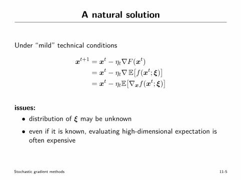
A natural solution
Under “mild” technical conditions
xt+1 = xt − ηt∇F (xt)= xt − ηt∇E
[f(xt; ξ)
]
= xt − ηtE[∇xf(xt; ξ)
]
issues:• distribution of ξ may be unknown• even if it is known, evaluating high-dimensional expectation is
often expensive
Stochastic gradient methods 11-5
Stochastic gradient descent(stochastic approximation)
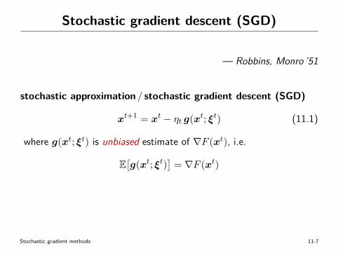
Stochastic gradient descent (SGD)
— Robbins, Monro ’51
stochastic approximation / stochastic gradient descent (SGD)
xt+1 = xt − ηt g(xt; ξt) (11.1)
where g(xt; ξt) is unbiased estimate of ∇F (xt), i.e.
E[g(xt; ξt)
]= ∇F (xt)
• a stochastic algorithm for finding a critical point x obeying∇F (x) = 0
• more generally, a stochastic algorithm for finding the roots ofG(x) := E[g(x; ξ)]
Stochastic gradient methods 11-7
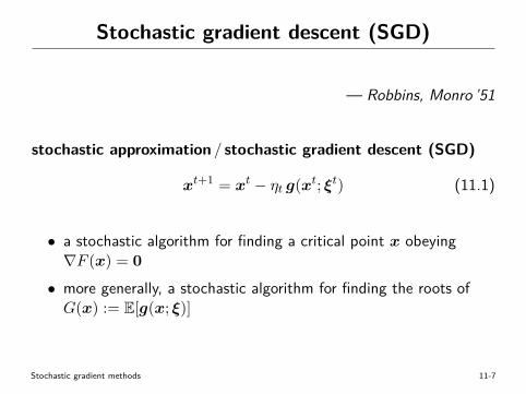
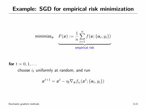
Example: SGD for empirical risk minimization
minimizex F (x) := 1n
n∑
i=1f(x; {ai, yi}
)
︸ ︷︷ ︸empirical risk
for t = 0, 1, . . .choose it uniformly at random, and run
xt+1 = xt − ηt∇xfit(xt; {ai, yi})
Stochastic gradient methods 11-8
Example: SGD for empirical risk minimization
benefits: SGD exploits information more efficiently than batchmethods• practical data usually involve lots of redundancy; using all data
simultaneously in each iteration might be inefficient• SGD is particularly efficient at the very beginning, as it achieves
fast initial improvement with very low per-iteration cost
Stochastic gradient methods 11-9
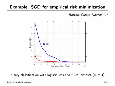
Example: SGD for empirical risk minimization— Bottou, Curtis, Nocedal ’18
0 0.5 1 1.5 2 2.5 3 3.5 4
x 105
0
0.1
0.2
0.3
0.4
0.5
0.6
Accessed Data Points
Em
piri
ca
l Ris
k
SGD
LBFGS
4
Fig. 3.1: Empirical risk Rn as a function of the number of accessed data points (ADP) for a batchL-BFGS method and the stochastic gradient (SG) method (3.7) on a binary classification problemwith a logistic loss objective and the RCV1 dataset. SG was run with a fixed stepsize of ↵ = 4.
w1 −1 w1,* 1
Fig. 3.2: Simple illustration to motivate the fast initial behavior of the SG method for minimizingempirical risk (3.6), where each fi is a convex quadratic. This example is adapted from [15].
convergence by employing a sequence of diminishing stepsizes to overcome any oscillatory behaviorof the algorithm.
Theoretical Motivation One can also cite theoretical arguments for a preference of SG over abatch approach. Let us give a preview of these arguments now, which are studied in more depthand further detail in §4.
• It is well known that a batch approach can minimize Rn at a fast rate; e.g., if Rn is stronglyconvex (see Assumption 4.5) and one applies a batch gradient method, then there exists aconstant ⇢ 2 (0, 1) such that, for all k 2 N, the training error satisfies
Rn(wk)�R⇤n O(⇢k), (3.9)
where R⇤n denotes the minimal value of Rn. The rate of convergence exhibited here is refereed
to as R-linear convergence in the optimization literature [117] and geometric convergence inthe machine learning research community; we shall simply refer to it as linear convergence.From (3.9), one can conclude that, in the worst case, the total number of iterations in whichthe training error can be above a given ✏ > 0 is proportional to log(1/✏). This means that, with
18
binary classification with logistic loss and RCV1 dataset (ηt ≡ 4)
Stochastic gradient methods 11-10
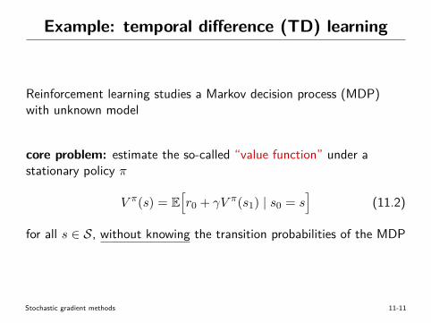
Example: temporal difference (TD) learning
Reinforcement learning studies a Markov decision process (MDP)with unknown model
core problem: estimate the so-called “value function” under astationary policy π
V π(s) = E[r0 + γV π(s1) | s0 = s
](11.2)
for all s ∈ S, without knowing the transition probabilities of the MDP
Stochastic gradient methods 11-11
Example: temporal difference (TD) learning
We won’t explain what Equation (11.2) means, but remark that . . .
• V π(·): value function under policy π• st: state at time t• S: state space• 0 < γ < 1: discount factor• rt: reward at time t
Stochastic gradient methods 11-12
Example: temporal difference (TD) learning
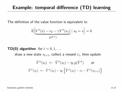
The definition of the value function is equivalent to
E[V π(s)− r0 − γV π(s1)︸ ︷︷ ︸
g(V π)
| s0 = s]
= 0
TD(0) algorithm: for t = 0, 1, . . .draw a new state st+1, collect a reward rt, then update
V π(st) ← V π(st)− ηt g(V π) or
V π(st) ← V π(st)− ηt{V π(st)− rt − V π(st+1)
}
Stochastic gradient methods 11-13
Example: Q-learning
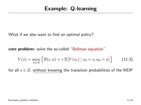
What if we also want to find an optimal policy?
core problem: solve the so-called “Bellman equation”
V (s) = maxa∈A
{R(s, a) + γ E
[V (s1) | s0 = s, a0 = a
]}(11.3)
for all s ∈ S, without knowing the transition probabilities of the MDP
Stochastic gradient methods 11-14
Example: Q-learning
Again we won’t explain what the Bellman equation means, butremark that . . .
• V (·): value function• st: state at time t• S: state space• at: action at time t• A: action space• 0 < γ < 1: discount factor• R(·, ·): reward function
Stochastic gradient methods 11-15
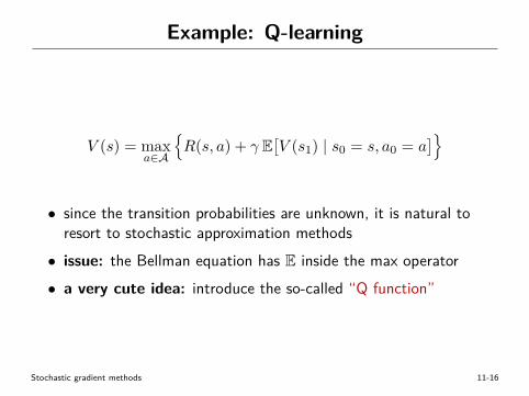
Example: Q-learning
V (s) = maxa∈A
{R(s, a) + γ E
[V (s1) | s0 = s, a0 = a
]}
• since the transition probabilities are unknown, it is natural toresort to stochastic approximation methods• issue: the Bellman equation has E inside the max operator• a very cute idea: introduce the so-called “Q function”
Stochastic gradient methods 11-16
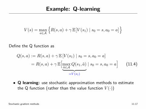
Example: Q-learning
V (s) = maxa∈A
{R(s, a) + γ E
[V (s1) | s0 = s, a0 = a
]}
Define the Q function as
Q(s, a) := R(s, a) + γ E [V (s1) | s0 = s, a0 = a]
= R(s, a) + γ E[maxa∈A
Q(s1, a)︸ ︷︷ ︸
=V (s1)
| s0 = s, a0 = a]
(11.4)
• Q learning: use stochastic approximation methods to estimatethe Q function (rather than the value function V (·))
Stochastic gradient methods 11-17
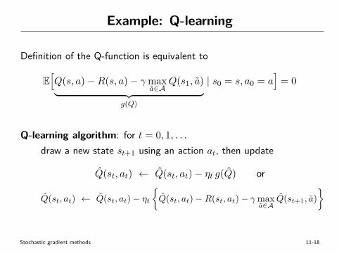
Example: Q-learning
Definition of the Q-function is equivalent to
E[Q(s, a)−R(s, a)− γmax
a∈AQ(s1, a)
︸ ︷︷ ︸g(Q)
| s0 = s, a0 = a]
= 0
Q-learning algorithm: for t = 0, 1, . . .draw a new state st+1 using an action at, then update
Q(st, at) ← Q(st, at)− ηt g(Q) or
Q(st, at) ← Q(st, at)− ηt{Q(st, at)−R(st, at)− γmax
a∈AQ(st+1, a)
}
Stochastic gradient methods 11-18
Convergence analysis
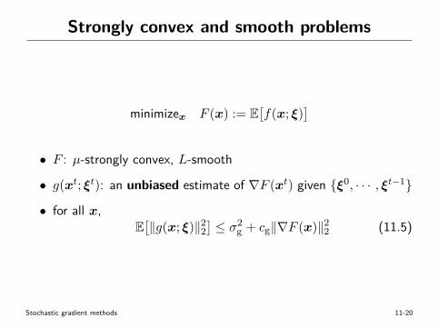
Strongly convex and smooth problems
minimizex F (x) := E[f(x; ξ)
]
• F : µ-strongly convex, L-smooth
• g(xt; ξt): an unbiased estimate of ∇F (xt) given {ξ0, · · · , ξt−1}
• for all x,E[‖g(x; ξ)‖22
] ≤ σ2g + cg‖∇F (x)‖22 (11.5)
Stochastic gradient methods 11-20
Convergence: fixed stepsizes
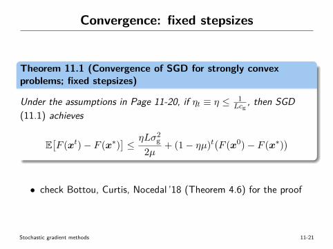
Theorem 11.1 (Convergence of SGD for strongly convexproblems; fixed stepsizes)
Under the assumptions in Page 11-20, if ηt ≡ η ≤ 1Lcg
, then SGD(11.1) achieves
E[F (xt)− F (x∗)
] ≤ ηLσ2g
2µ + (1− ηµ)t(F (x0)− F (x∗)
)
• check Bottou, Curtis, Nocedal ’18 (Theorem 4.6) for the proof
Stochastic gradient methods 11-21
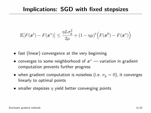
Implications: SGD with fixed stepsizes
E[F (xt)− F (x∗)
] ≤ ηLσ2g
2µ + (1− ηµ)t(F (x0)− F (x∗)
)
• fast (linear) convergence at the very beginning• converges to some neighborhood of x∗ — variation in gradient
computation prevents further progress• when gradient computation is noiseless (i.e. σg = 0), it converges
linearly to optimal points• smaller stepsizes η yield better converging points
Stochastic gradient methods 11-22
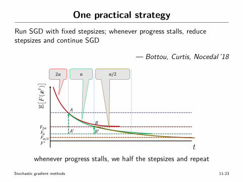
One practical strategyRun SGD with fixed stepsizes; whenever progress stalls, reducestepsizes and continue SGD
— Bottou, Curtis, Nocedal ’18
of stepsize decrease, we may invoke Theorem 4.6, from which it follows that to achieve the firstbound in (4.17) one needs
(1� ↵rcµ)(kr+1�kr)(4F↵r � F↵r) F↵r
=) kr+1 � kr �log(1/3)
log(1� ↵rcµ)⇡ log(3)
↵rcµ= O(2r).
(4.18)
In other words, each time the stepsize is cut in half, double the number of iterations are required.This is a sublinear rate of stepsize decrease—e.g., if {kr} = {2r�1}, then ↵k = ↵1/k for all k 2{2r}—which, from {F↵r} = {↵rLM
2cµ } and (4.17), means that a sublinear convergence rate of thesuboptimality gap is achieved.
!"
#$
!
%#& '
#(#$)*
" ")!
+
+,--,
Fig. 4.1: Depiction of the strategy of halving the stepsize ↵ when the expected suboptimality gapis smaller than twice the asymptotic limit F↵. In the figure, the segment B–B0 has one third of thelength of A–A0. This is the amount of decrease that must be made in the exponential term in (4.14)by raising the contraction factor to the power of the number of steps during which one maintainsa given constant stepsize; see (4.18). Since the contraction factor is (1�↵cµ), the number of stepsmust be proportional to ↵. Therefore, whenever the stepsize is halved, one must maintain it twiceas long. Overall, doubling the number of iterations halves the suboptimality gap each time, yieldingan e↵ective rate of O(1/k).
In fact, these conclusions can be obtained in a more rigorous manner that also allows moreflexibility in the choice of stepsize sequence. The following result harks back to the seminal workof Robbins and Monro [130], where the stepsize requirement takes the form
1X
k=1
↵k =1 and
1X
k=1
↵2k <1. (4.19)
Theorem 4.7 (Strongly Convex Objective, Diminishing Stepsizes). Under Assumptions 4.1,4.3, and 4.5 (with Finf = F⇤), suppose that the SG method (Algorithm 4.1) is run with a stepsizesequence such that, for all k 2 N,
↵k =�
� + kfor some � >
1
cµand � > 0 such that ↵1
µ
LMG. (4.20)
28
Convergence analysisUsing Lemma 5.4, we immediate arrive atTheorem 5.3
Suppose f is convex and Lipschitz continuous (i.e. ÎgtÎú Æ Lf ) on C,and suppoe Ï is fl-strongly convex w.r.t. Î · Î. Then
fbest,t ≠ fopt ÆsupxœC DÏ
!x,x0"
+ L2f
2fl
qtk=0 ÷2
kqtk=0 ÷k
• If ÷t =Ô
2flRLf
1Ôt
with R := supxœC DÏ!x,x0"
, then
fbest,t ≠ fopt Æ O
ALf
ÔRÔ
fl
log tÔt
B
¶ one can further remove log t factorMirror descent 5-37
1 t
t�2
X j=
0
A�
1⇠
jd !
N� 0
,A�
1S
A�
1�
kGt 0k
<1
,kG
t j�
A�
1k
1,
and
lim
t!1
1 t
t�1
X j=
0
kGt j�
A�
1k
=0
iter
atio
npe
r-iter
atio
nto
tal
com
plex
ity
cost
com
put.
cost
batc
hG
Dlo
g1 ✏
nn
log
1 ✏
SGD
1 ✏1
1 ✏
E⇥ F(x
t)�
F(x
⇤ )⇤
⌘L
M
2µ
+(1
�⌘µ)t⇣ F
(x0)�
F(x
⇤ )⌘
E⇥ F(x
t)⇤
8
whenever progress stalls, we half the stepsizes and repeat
Stochastic gradient methods 11-23
Convergence with diminishing stepsizes
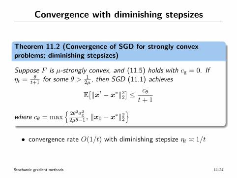
Theorem 11.2 (Convergence of SGD for strongly convexproblems; diminishing stepsizes)
Suppose F is µ-strongly convex, and (11.5) holds with cg = 0. Ifηt = θ
t+1 for some θ > 12µ , then SGD (11.1) achieves
E[‖xt − x∗‖22
] ≤ cθt+ 1
where cθ = max{ 2θ2σ2
g2µθ−1 , ‖x0 − x∗‖22
}
• convergence rate O(1/t) with diminishing stepsize ηt � 1/t
Stochastic gradient methods 11-24
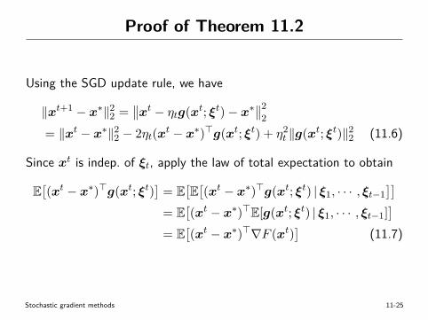
Proof of Theorem 11.2
Using the SGD update rule, we have
‖xt+1 − x∗‖22 =∥∥xt − ηtg(xt; ξt)− x∗
∥∥22
= ‖xt − x∗‖22 − 2ηt(xt − x∗)>g(xt; ξt) + η2t ‖g(xt; ξt)‖22 (11.6)
Since xt is indep. of ξt, apply the law of total expectation to obtain
E[(xt − x∗)>g(xt; ξt)
]= E
[E[(xt − x∗)>g(xt; ξt) | ξ1, · · · , ξt−1
]]
= E[(xt − x∗)>E[g(xt; ξt) | ξ1, · · · , ξt−1]
]
= E[(xt − x∗)>∇F (xt)
](11.7)
Stochastic gradient methods 11-25
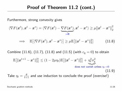
Proof of Theorem 11.2 (cont.)
Furthermore, strong convexity gives
〈∇F (xt),xt − x∗〉 = 〈∇F (xt)−∇F (x∗)︸ ︷︷ ︸=0
,xt − x∗〉 ≥ µ∥∥xt − x∗
∥∥22
=⇒ E[〈∇F (xt),xt − x∗〉] ≥ µE[‖xt − x∗‖22
](11.8)
Combine (11.6), (11.7), (11.8) and (11.5) (with cg = 0) to obtain
E[‖xt+1 − x∗‖22
] ≤ (1− 2µηt)E[‖xt − x∗‖22
]+ η2
t σ2g︸ ︷︷ ︸
does not vanish unless ηt→0(11.9)
Take ηt = θt+1 and use induction to conclude the proof (exercise!)
Stochastic gradient methods 11-26
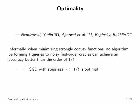
Optimality
— Nemirovski, Yudin ’83, Agarwal et al. ’11, Raginsky, Rakhlin ’11
Informally, when minimizing strongly convex functions, no algorithmperforming t queries to noisy first-order oracles can achieve anaccuracy better than the order of 1/t
=⇒ SGD with stepsizes ηt � 1/t is optimal
Stochastic gradient methods 11-27
Optimality
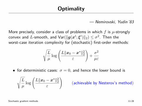
— Nemirovski, Yudin ’83
More precisely, consider a class of problems in which f is µ-stronglyconvex and L-smooth, and Var(‖g(xt; ξt)‖2) ≤ σ2. Then theworst-case iteration complexity for (stochastic) first-order methods:
√L
µlog
(L‖x0 − x∗‖22
ε
)+ σ2
µε
• for deterministic cases: σ = 0, and hence the lower bound is√L
µlog
(L‖x0 − x∗‖22
ε
)(achievable by Nesterov’s method)
• for noisy cases with large σ, the lower bound is dominated by
σ2
µ· 1ε
Stochastic gradient methods 11-28
Optimality
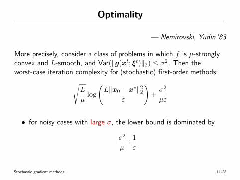
— Nemirovski, Yudin ’83
More precisely, consider a class of problems in which f is µ-stronglyconvex and L-smooth, and Var(‖g(xt; ξt)‖2) ≤ σ2. Then theworst-case iteration complexity for (stochastic) first-order methods:
√L
µlog
(L‖x0 − x∗‖22
ε
)+ σ2
µε
• for deterministic cases: σ = 0, and hence the lower bound is√L
µlog
(L‖x0 − x∗‖22
ε
)(achievable by Nesterov’s method)
• for noisy cases with large σ, the lower bound is dominated by
σ2
µ· 1ε
Stochastic gradient methods 11-28
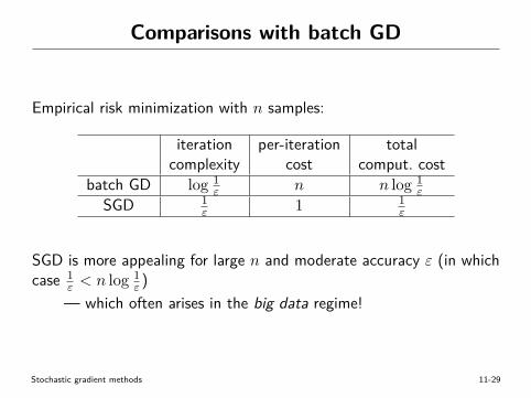
Comparisons with batch GD
Empirical risk minimization with n samples:
iteration per-iteration totalcomplexity cost comput. cost
batch GD log 1ε n n log 1
ε
SGD 1ε 1 1
ε
SGD is more appealing for large n and moderate accuracy ε (in whichcase 1
ε < n log 1ε )
— which often arises in the big data regime!
Stochastic gradient methods 11-29
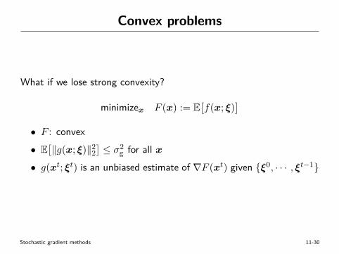
Convex problems
What if we lose strong convexity?
minimizex F (x) := E[f(x; ξ)
]
• F : convex• E
[‖g(x; ξ)‖22] ≤ σ2
g for all x• g(xt; ξt) is an unbiased estimate of ∇F (xt) given {ξ0, · · · , ξt−1}
Stochastic gradient methods 11-30
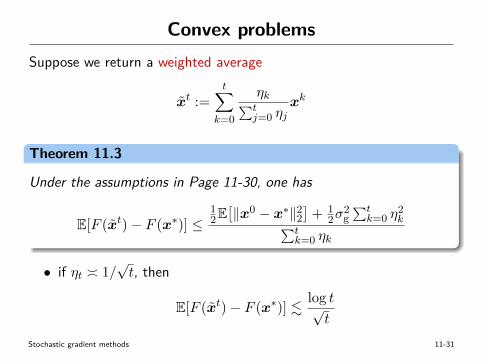
Convex problemsSuppose we return a weighted average
xt :=t∑
k=0
ηk∑tj=0 ηj
xk
Theorem 11.3
Under the assumptions in Page 11-30, one has
E[F (xt)− F (x∗)] ≤12E[‖x0 − x∗‖22
]+ 1
2σ2g∑tk=0 η
2k∑t
k=0 ηk
• if ηt � 1/√t, then
E[F (xt)− F (x∗)] . log t√t
Stochastic gradient methods 11-31
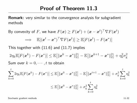
Proof of Theorem 11.3Remark: very similar to the convergence analysis for subgradientmethods
By convexity of F , we have F (x) ≥ F (xt) + (x− xt)>∇F (xt)
=⇒ E[(xt − x∗)>∇F (xt)] ≥ E[F (xt)− F (x∗)]
This together with (11.6) and (11.7) implies
2ηkE[F (xk)− F (x∗)] ≤ E[‖xk − x∗‖22
]− E[‖xk+1 − x∗‖22
]+ η2
kσ2g
Sum over k = 0, · · · , t to obtaint∑
k=02ηkE[F (xk)− F (x∗)] ≤ E
[‖x0 − x∗‖2
2]− E
[‖xt+1 − x∗‖2
2]
+ σ2g
t∑
k=0η2k
≤ E[‖x0 − x∗‖2
2]
+ σ2g
t∑
k=0η2k
Stochastic gradient methods 11-32
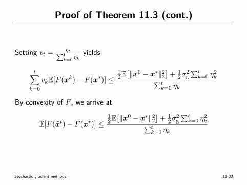
Proof of Theorem 11.3 (cont.)
Setting vt = ηt∑t
k=0 ηkyields
t∑
k=0vkE[F (xk)− F (x∗)] ≤
12E[‖x0 − x∗‖22
]+ 1
2σ2g∑tk=0 η
2k∑t
k=0 ηk
By convexity of F , we arrive at
E[F (xt)− F (x∗)] ≤12E[‖x0 − x∗‖22
]+ 1
2σ2g∑tk=0 η
2k∑t
k=0 ηk
Stochastic gradient methods 11-33
Reducing variance via iterate averaging
Stepsize choice O(1/t)?
Two conflicting regimes• the noiseless case (i.e. g(x; ξ) = ∇F (x)): stepsizes ηt � 1/t are
way too conservative
• the general noisy case: longer stepsizes (ηt � 1/t) might fail tosuppress noise (and hence slow down convergence)
Can we modify SGD so as to allow for larger stepsizeswithout compromising convergence rates?
Stochastic gradient methods 11-35
Motivation for iterate averaging
SGD with long stepsizes poorly suppresses noise, which tends tooscillate around the global minimizers due to the noisy nature ofgradient computation
One may, however, average iterates to mitigate oscillation and reducevariance
Stochastic gradient methods 11-36
Acceleration by averaging
— Ruppert ’88, Polyak ’90, Polyak, Juditsky ’92
return xt := 1t
t−1∑
i=0xi (11.10)
with larger stepsizes ηt � t−α, α < 1
Key idea: average the iterates to reduce variance and improveconvergence
Stochastic gradient methods 11-37
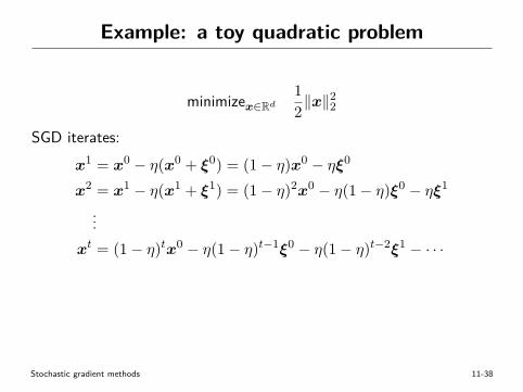
Example: a toy quadratic problem
minimizex∈Rd12‖x‖
22
• constant stepsizes: ηt ≡ η < 1
• g(xt; ξt) = xt + ξt with◦ E
[ξt | ξ0, · · · , ξt−1] = 0
◦ E[ξtξt> | ξ0, · · · , ξt−1] = I
SGD iterates:x1 = x0 − η(x0 + ξ0) = (1− η)x0 − ηξ0
x2 = x1 − η(x1 + ξ1) = (1− η)2x0 − η(1− η)ξ0 − ηξ1
...xt = (1− η)tx0 − η(1− η)t−1ξ0 − η(1− η)t−2ξ1 − · · ·
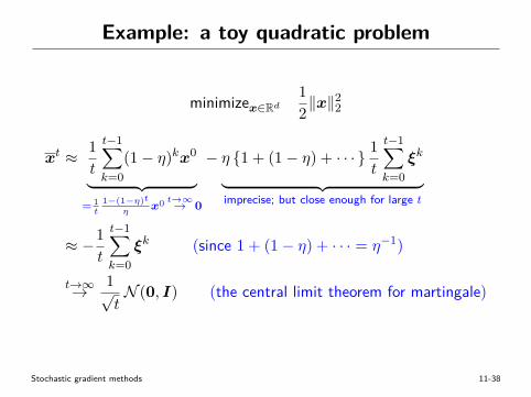
xt ≈ 1t
t−1∑
k=0(1− η)kx0
︸ ︷︷ ︸= 1t
1−(1−η)tη
x0 t→∞→ 0
− η {1 + (1− η) + · · · } 1t
t−1∑
k=0ξk
︸ ︷︷ ︸imprecise; but close enough for large t
≈ −1t
t−1∑
k=0ξk (since 1 + (1− η) + · · · = η−1)
t→∞→ 1√tN (0, I) (the central limit theorem for martingale)
Stochastic gradient methods 11-38
Example: a toy quadratic problem
minimizex∈Rd12‖x‖
22
• constant stepsizes: ηt ≡ η < 1
• g(xt; ξt) = xt + ξt with◦ E
[ξt | ξ0, · · · , ξt−1] = 0
◦ E[ξtξt> | ξ0, · · · , ξt−1] = I
SGD iterates:x1 = x0 − η(x0 + ξ0) = (1− η)x0 − ηξ0
x2 = x1 − η(x1 + ξ1) = (1− η)2x0 − η(1− η)ξ0 − ηξ1
...xt = (1− η)tx0 − η(1− η)t−1ξ0 − η(1− η)t−2ξ1 − · · ·
xt ≈ 1t
t−1∑
k=0(1− η)kx0
︸ ︷︷ ︸= 1t
1−(1−η)tη
x0 t→∞→ 0
− η {1 + (1− η) + · · · } 1t
t−1∑
k=0ξk
︸ ︷︷ ︸imprecise; but close enough for large t
≈ −1t
t−1∑
k=0ξk (since 1 + (1− η) + · · · = η−1)
t→∞→ 1√tN (0, I) (the central limit theorem for martingale)
Stochastic gradient methods 11-38
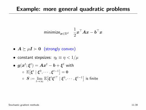
Example: more general quadratic problems
minimizex∈Rd12x>Ax− b>x
• A � µI � 0 (strongly convex)
• constant stepsizes: ηt ≡ η < 1/µ
• g(xt; ξt) = Axt − b+ ξt with◦ E
[ξt | ξ0, · · · , ξt−1] = 0
◦ S := limt→∞
E[ξtξt> | ξ0, · · · , ξt−1] is finite
Theorem 11.4
Fix d. Then as t→∞, the iterate average xt obeys√t(xt − x∗) D→︸︷︷︸
convergence in distribution
N (0,A−1SA−1)
Stochastic gradient methods 11-39
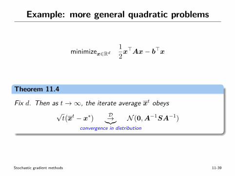
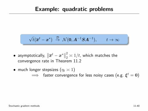
Example: quadratic problems
√t(xt − x∗) D→ N (0,A−1SA−1), t→∞
• asymptotically,∥∥xt − x∗
∥∥22 � 1/t, which matches the
convergence rate in Theorem 11.2
• much longer stepsizes (ηt � 1)=⇒ faster convergence for less noisy cases (e.g. ξt = 0)
Stochastic gradient methods 11-40
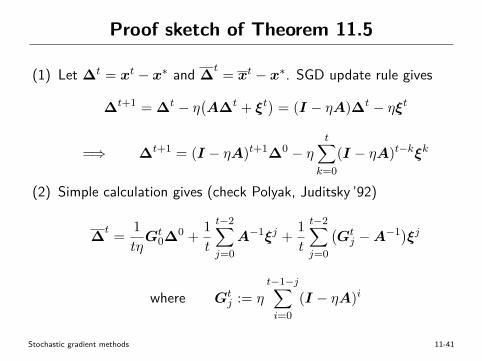
Proof sketch of Theorem 11.5
(1) Let ∆t = xt − x∗ and ∆t = xt − x∗. SGD update rule gives
∆t+1 = ∆t − η(A∆t + ξt)
= (I − ηA)∆t − ηξt
=⇒ ∆t+1 = (I − ηA)t+1∆0 − ηt∑
k=0(I − ηA)t−kξk
(2) Simple calculation gives (check Polyak, Juditsky ’92)
∆t = 1
tηGt
0∆0 + 1
t
t−2∑
j=0A−1ξj + 1
t
t−2∑
j=0
(Gtj −A−1)ξj
where Gtj := η
t−1−j∑
i=0(I − ηA)i
Stochastic gradient methods 11-41
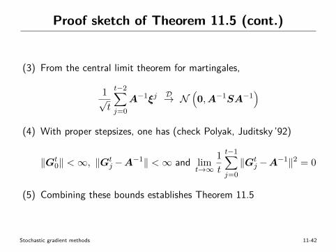
Proof sketch of Theorem 11.5 (cont.)
(3) From the central limit theorem for martingales,
1√t
t−2∑
j=0A−1ξj
D→ N(0,A−1SA−1
)
(4) With proper stepsizes, one has (check Polyak, Juditsky ’92)
‖Gt0‖ <∞, ‖Gt
j −A−1‖ <∞ and limt→∞
1t
t−1∑
j=0‖Gt
j −A−1‖2 = 0
(5) Combining these bounds establishes Theorem 11.5
Stochastic gradient methods 11-42
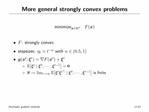
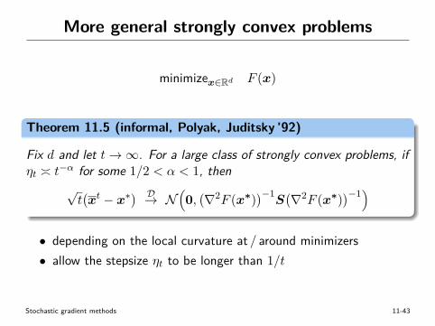
More general strongly convex problems
minimizex∈Rd F (x)
• F : strongly convex
• stepsizes: ηt � t−α with α ∈ (0.5, 1)
• g(xt; ξt) = ∇F (xt) + ξt
◦ E[ξt | ξ0, · · · , ξt−1] = 0
◦ S := limt→∞ E[ξtξt> | ξ0, · · · , ξt−1] is finite
Theorem 11.5 (informal, Polyak, Juditsky ’92)
Fix d and let t→∞. For a large class of strongly convex problems, ifηt � t−α for some 1/2 < α < 1, then
√t(xt − x∗) D→ N
(0,(∇2F (x∗)
)−1S(∇2F (x∗)
)−1)
• depending on the local curvature at / around minimizers• allow the stepsize ηt to be longer than 1/t
Stochastic gradient methods 11-43
Reference
[1] ”A stochastic approximation method, H. Robbins, S. Monro, the annalsof mathematical statistics, 1951.
[2] ”Robust stochastic approximation approach to stochastic programming,”A. Nemirovski et al., SIAM Journal on optimization, 2009.
[3] ”Optimization methods for large-scale machine learning,” L. Bottou etal., arXiv, 2016.
[4] ”New stochastic approximation type procedures,” B. Polyak, Automat.Remote Control, 1990.
[5] ”Acceleration of stochastic approximation by averaging,” B. Polyak,A. Juditsky, SIAM Journal on Control and Optimization, 1992.
[6] ”Efficient estimations from a slowly convergent Robbins-Monro process,”D. Ruppert, 1988.
Stochastic gradient methods 11-44
Reference[7] ”Problem complexity and method efficiency in optimization,”
A. Nemirovski, D. Yudin, Wiley, 1983.[8] ”Information-theoretic lower bounds on the oracle complexity of
stochastic convex optimization,” A. Agarwal, P. Bartlett, P. Ravikumar,M. Wainwright, IEEE Transactions on Information Theory, 2011.
[9] ”Information-based complexity, feedback and dynamics in convexprogramming,” M. Raginsky, A. Rakhlin, IEEE Transactions onInformation Theory, 2011.
[10] ”First-order methods in optimization,” A. Beck, Vol. 25, SIAM, 2017.[11] ”Acceleration of stochastic approximation by averaging,” B. Polyak,
A. Juditsky, SIAM Journal on Control and Optimization, 1992.[12] ”A convergence theorem for nonnegative almost supermartingales and
some applications,” H. Robbins, D. Siegmund, Optimizing methods instatistics, 1971.
Stochastic gradient methods 11-45