Stochastic Calculus Main Results - Department of Statistical Sciences
18
1 MMF1952Y: Stochastic Calculus Main Results © 2006 Prof. S. Jaimungal Department of Statistics and Mathematical Finance Program University of Toronto © S. Jaimungal, 2006 2 Probability Spaces A probability space is a triple (Ω, P , F ) where Ω is the set of all possible outcomes P is a probability measure F is a sigma-algebra telling us which (c) Sebastian Jaimungal, 2009
Transcript of Stochastic Calculus Main Results - Department of Statistical Sciences

1
MMF1952Y:Stochastic Calculus Main Results
© 2006 Prof. S. Jaimungal
Department of Statistics and
Mathematical Finance Program
University of Toronto
© S. Jaimungal, 2006 2
Probability Spaces
A probability space is a triple (Ω, P , F ) where
Ω is the set of all possible outcomes
P is a probability measure
F is a sigma-algebra telling us which
(c) Sebastian Jaimungal, 2009
2
© S. Jaimungal, 2006 3
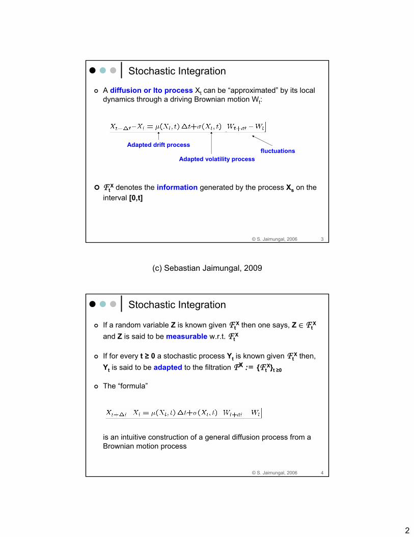
Stochastic Integration
A diffusion or Ito process Xt can be “approximated” by its local dynamics through a driving Brownian motion Wt:
FtX denotes the information generated by the process Xs on the
interval [0,t]
Adapted drift process
Adapted volatility processfluctuations
© S. Jaimungal, 2006 4
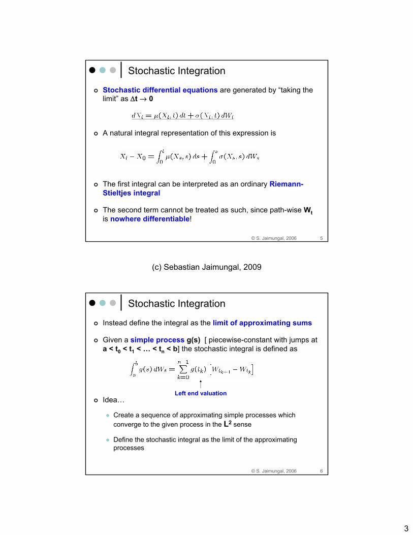
Stochastic Integration
If a random variable Z is known given FtX then one says, Z ∈ Ft
X
and Z is said to be measurable w.r.t. FtX
If for every t ≥ 0 a stochastic process Yt is known given FtX then,
Yt is said to be adapted to the filtration FX := {FtX}t ≥0
The “formula”
is an intuitive construction of a general diffusion process from a Brownian motion process
(c) Sebastian Jaimungal, 2009
3
© S. Jaimungal, 2006 5
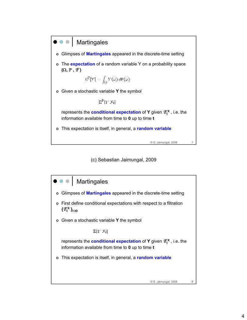
Stochastic Integration
Stochastic differential equations are generated by “taking the limit” as Δt → 0
A natural integral representation of this expression is
The first integral can be interpreted as an ordinary Riemann-Stieltjes integral
The second term cannot be treated as such, since path-wise Wtis nowhere differentiable!
© S. Jaimungal, 2006 6
Stochastic Integration
Instead define the integral as the limit of approximating sums
Given a simple process g(s) [ piecewise-constant with jumps at a < t0 < t1 < … < tn < b] the stochastic integral is defined as
Idea…
Create a sequence of approximating simple processes which converge to the given process in the L2 sense
Define the stochastic integral as the limit of the approximatingprocesses
Left end valuation
(c) Sebastian Jaimungal, 2009
4
© S. Jaimungal, 2006 7
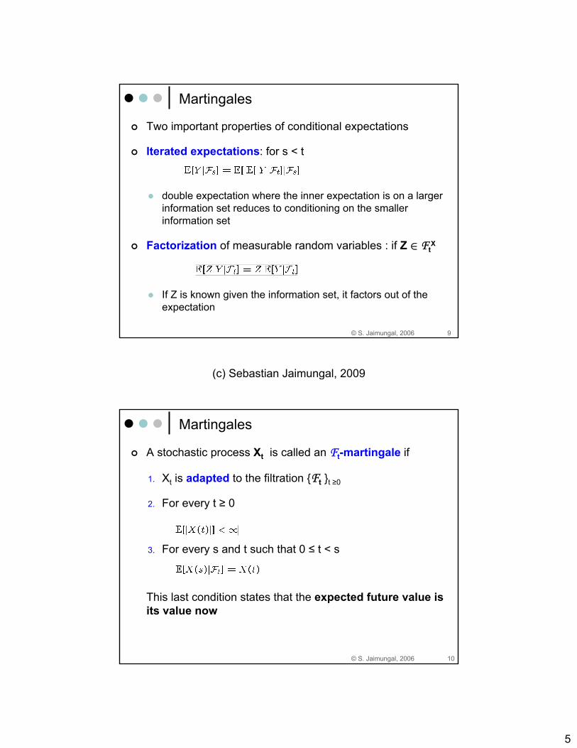
Martingales
Glimpses of Martingales appeared in the discrete-time setting
The expectation of a random variable Y on a probability space (Ω, P , F )
Given a stochastic variable Y the symbol
represents the conditional expectation of Y given FtX , i.e. the
information available from time to 0 up to time t
This expectation is itself, in general, a random variable
© S. Jaimungal, 2006 8
Martingales
Glimpses of Martingales appeared in the discrete-time setting
First define conditional expectations with respect to a filtration {Ft
X }t ≥0
Given a stochastic variable Y the symbol
represents the conditional expectation of Y given FtX , i.e. the
information available from time to 0 up to time t
This expectation is itself, in general, a random variable
(c) Sebastian Jaimungal, 2009
5
© S. Jaimungal, 2006 9
Martingales
Two important properties of conditional expectations
Iterated expectations: for s < t
double expectation where the inner expectation is on a larger information set reduces to conditioning on the smaller information set
Factorization of measurable random variables : if Z ∈ FtX
If Z is known given the information set, it factors out of the expectation
© S. Jaimungal, 2006 10
Martingales
A stochastic process Xt is called an Ft-martingale if
1. Xt is adapted to the filtration {Ft }t ≥0
2. For every t ≥ 0
3. For every s and t such that 0 ≤ t < s
This last condition states that the expected future value is its value now
(c) Sebastian Jaimungal, 2009
6
© S. Jaimungal, 2006 11
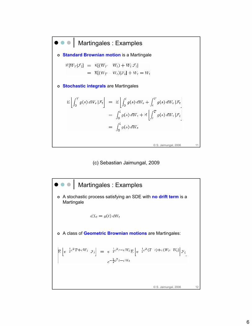
Martingales : Examples
Standard Brownian motion is a Martingale
Stochastic integrals are Martingales
© S. Jaimungal, 2006 12
Martingales : Examples
A stochastic process satisfying an SDE with no drift term is a Martingale
A class of Geometric Brownian motions are Martingales:
(c) Sebastian Jaimungal, 2009
7
© S. Jaimungal, 2006 13
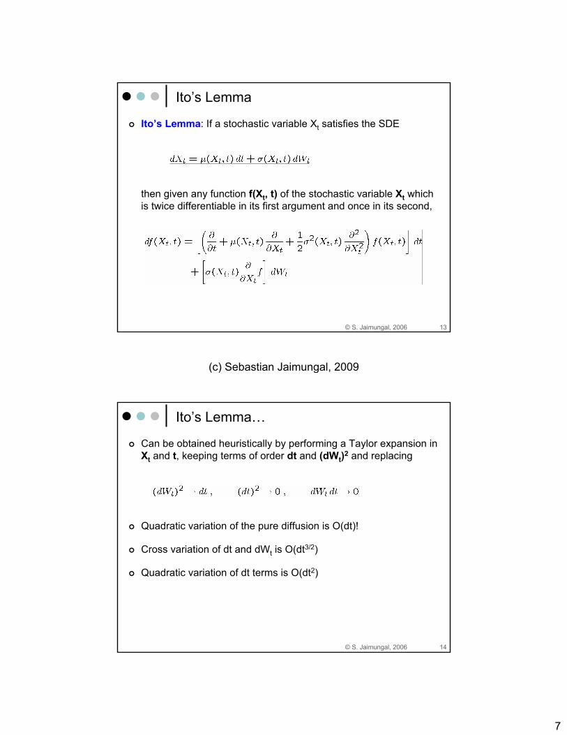
Ito’s Lemma
Ito’s Lemma: If a stochastic variable Xt satisfies the SDE
then given any function f(Xt, t) of the stochastic variable Xt which is twice differentiable in its first argument and once in its second,
© S. Jaimungal, 2006 14
Ito’s Lemma…
Can be obtained heuristically by performing a Taylor expansion in Xt and t, keeping terms of order dt and (dWt)2 and replacing
Quadratic variation of the pure diffusion is O(dt)!
Cross variation of dt and dWt is O(dt3/2)
Quadratic variation of dt terms is O(dt2)
(c) Sebastian Jaimungal, 2009
8
© S. Jaimungal, 2006 15
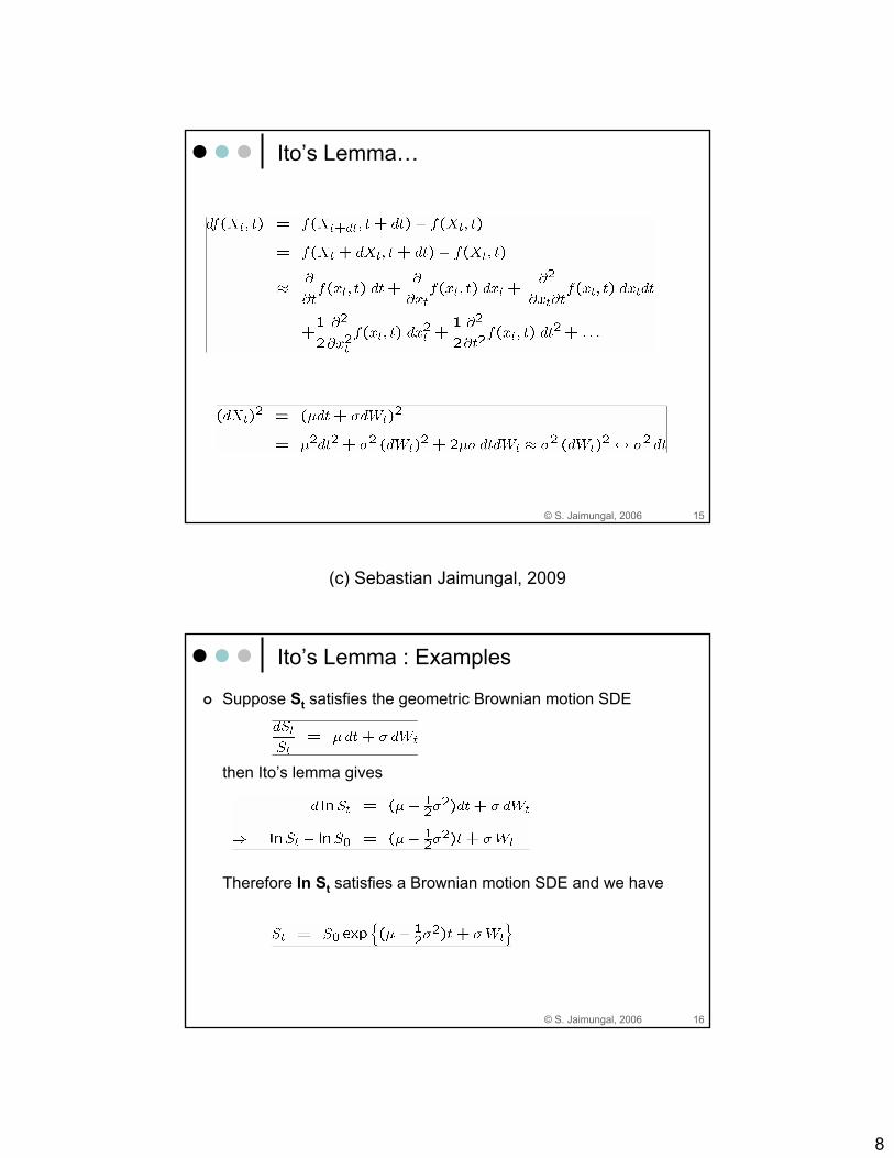
Ito’s Lemma…
© S. Jaimungal, 2006 16
Ito’s Lemma : Examples
Suppose St satisfies the geometric Brownian motion SDE
then Ito’s lemma gives
Therefore ln St satisfies a Brownian motion SDE and we have
(c) Sebastian Jaimungal, 2009
9
© S. Jaimungal, 2006 17
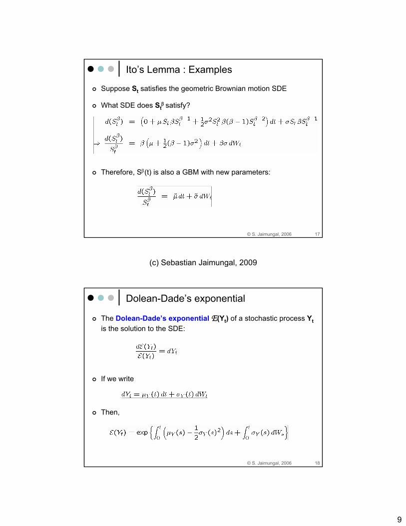
Ito’s Lemma : Examples
Suppose St satisfies the geometric Brownian motion SDE
What SDE does Stβ satisfy?
Therefore, Sβ(t) is also a GBM with new parameters:
© S. Jaimungal, 2006 18
Dolean-Dade’s exponential
The Dolean-Dade’s exponential E(Yt) of a stochastic process Ytis the solution to the SDE:
If we write
Then,
(c) Sebastian Jaimungal, 2009
10
© S. Jaimungal, 2006 19
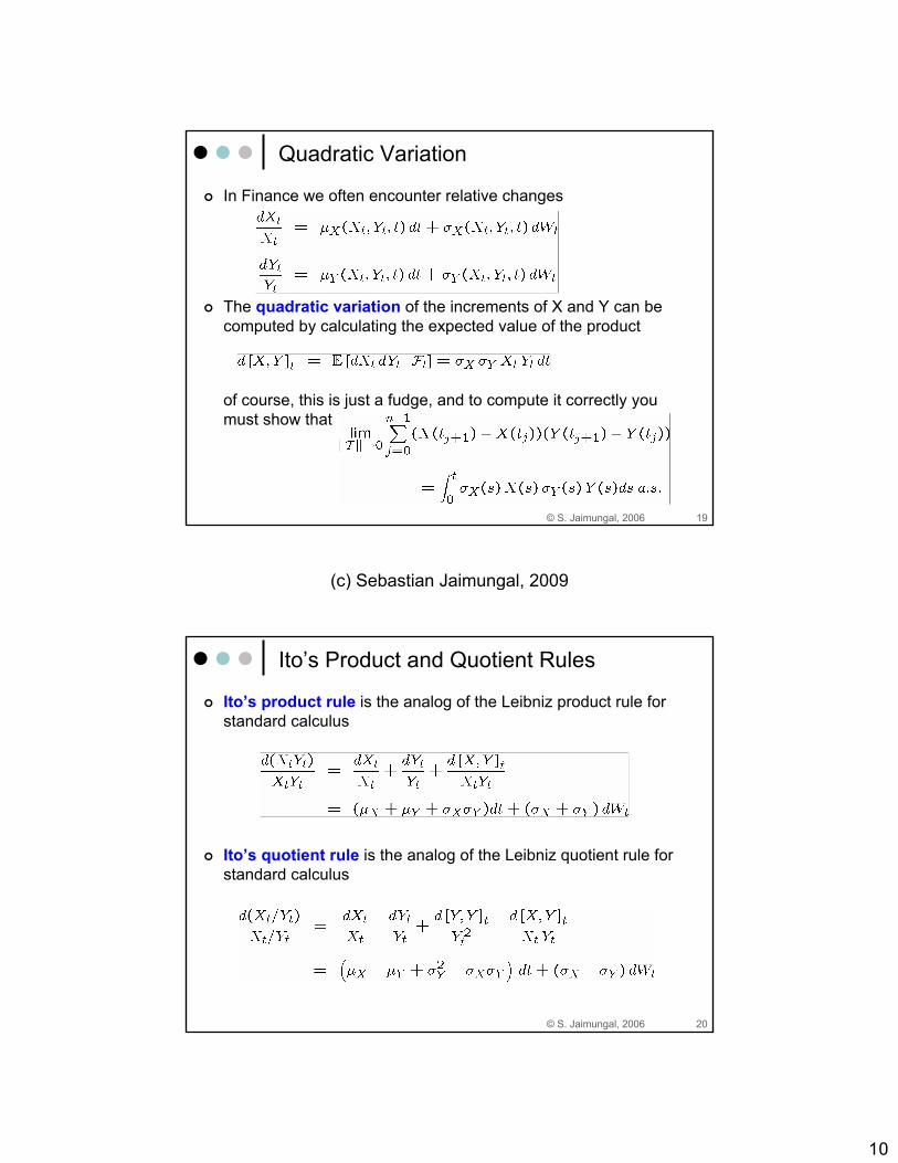
Quadratic Variation
In Finance we often encounter relative changes
The quadratic variation of the increments of X and Y can be computed by calculating the expected value of the product
of course, this is just a fudge, and to compute it correctly youmust show that
© S. Jaimungal, 2006 20
Ito’s Product and Quotient Rules
Ito’s product rule is the analog of the Leibniz product rule for standard calculus
Ito’s quotient rule is the analog of the Leibniz quotient rule for standard calculus
(c) Sebastian Jaimungal, 2009
11
© S. Jaimungal, 2006 21
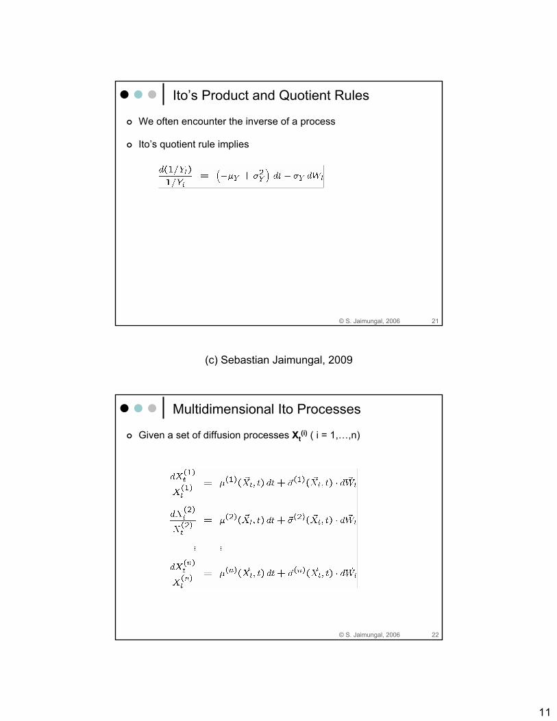
Ito’s Product and Quotient Rules
We often encounter the inverse of a process
Ito’s quotient rule implies
© S. Jaimungal, 2006 22
Multidimensional Ito Processes
Given a set of diffusion processes Xt(i) ( i = 1,…,n)
(c) Sebastian Jaimungal, 2009
12
© S. Jaimungal, 2006 23
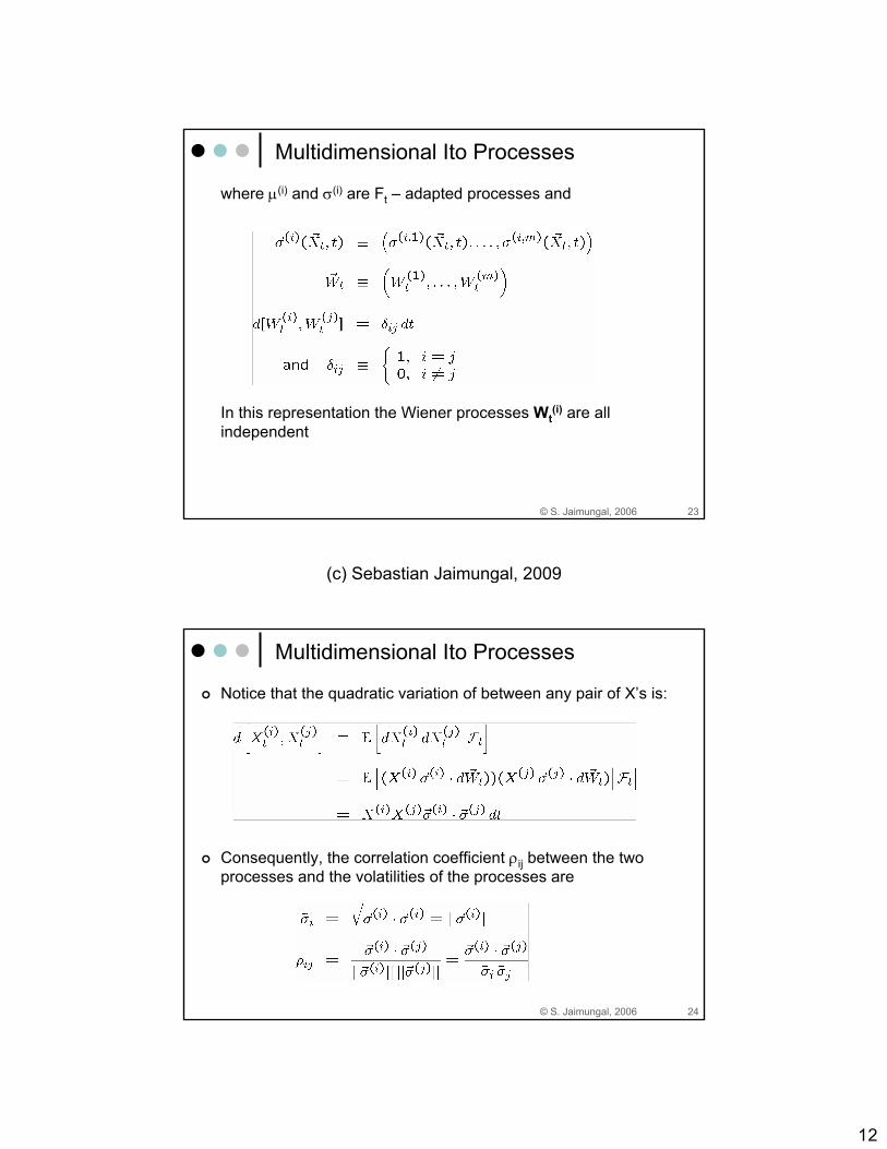
Multidimensional Ito Processes
where μ(i) and σ(i) are Ft – adapted processes and
In this representation the Wiener processes Wt(i) are all
independent
© S. Jaimungal, 2006 24
Multidimensional Ito Processes
Notice that the quadratic variation of between any pair of X’s is:
Consequently, the correlation coefficient ρij between the two processes and the volatilities of the processes are
(c) Sebastian Jaimungal, 2009
13
© S. Jaimungal, 2006 25
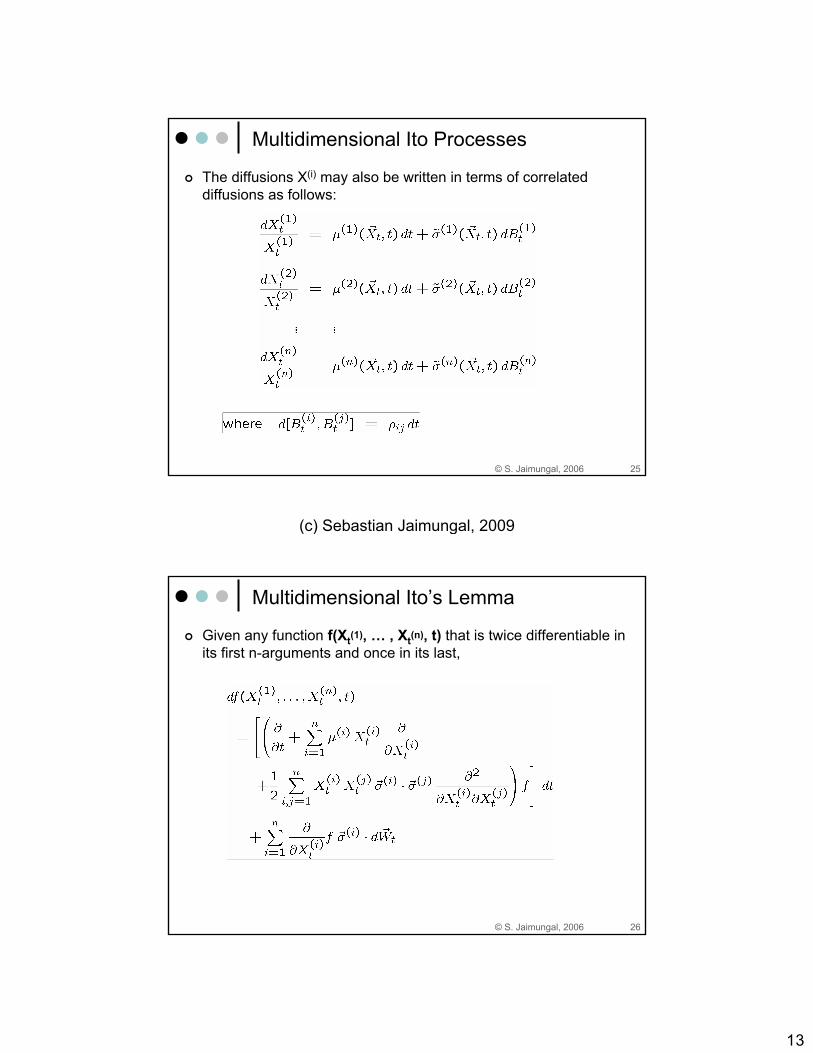
Multidimensional Ito Processes
The diffusions X(i) may also be written in terms of correlated diffusions as follows:
© S. Jaimungal, 2006 26
Multidimensional Ito’s Lemma
Given any function f(Xt(1), … , Xt(n), t) that is twice differentiable in its first n-arguments and once in its last,
(c) Sebastian Jaimungal, 2009
14
© S. Jaimungal, 2006 27
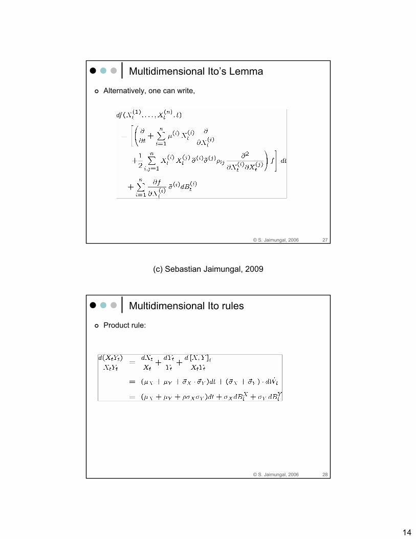
Multidimensional Ito’s Lemma
Alternatively, one can write,
© S. Jaimungal, 2006 28
Multidimensional Ito rules
Product rule:
(c) Sebastian Jaimungal, 2009
15
© S. Jaimungal, 2006 29
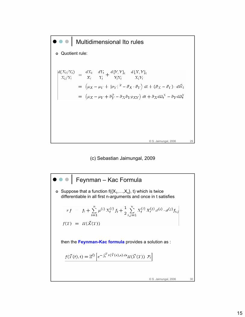
Multidimensional Ito rules
Quotient rule:
© S. Jaimungal, 2006 30
Feynman – Kac Formula
Suppose that a function f({X1,…,Xn}, t) which is twice differentiable in all first n-arguments and once in t satisfies
then the Feynman-Kac formula provides a solution as :
(c) Sebastian Jaimungal, 2009
16
© S. Jaimungal, 2006 31
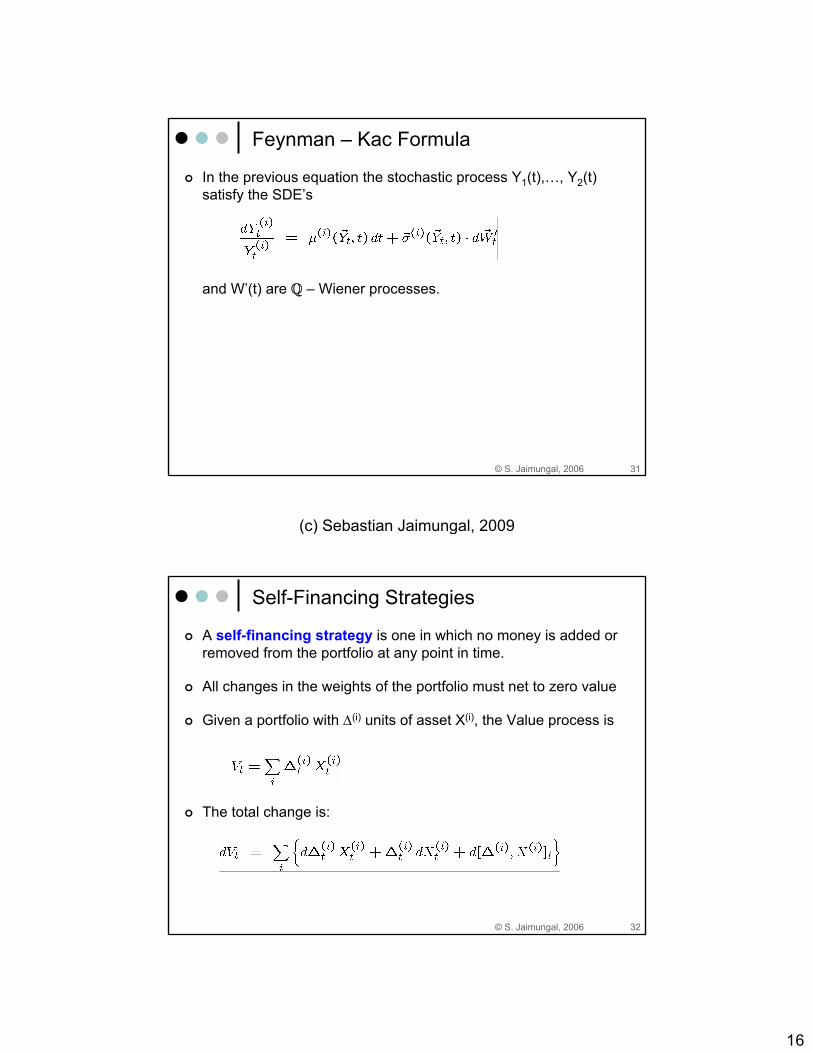
Feynman – Kac Formula
In the previous equation the stochastic process Y1(t),…, Y2(t) satisfy the SDE’s
and W’(t) are Q – Wiener processes.
© S. Jaimungal, 2006 32
Self-Financing Strategies
A self-financing strategy is one in which no money is added or removed from the portfolio at any point in time.
All changes in the weights of the portfolio must net to zero value
Given a portfolio with Δ(i) units of asset X(i), the Value process is
The total change is:
(c) Sebastian Jaimungal, 2009

17
© S. Jaimungal, 2006 33
Self-Financing Strategies
If the strategy is self-financing then,
So that self-financing requires,
© S. Jaimungal, 2006 34
Measure Changes
The Radon-Nikodym derivative connects probabilities in one measure P to probabilities in an equivalent measure Q
This random variable has P-expected value of 1
Its conditional expectation is a martingale process
(c) Sebastian Jaimungal, 2009
18
© S. Jaimungal, 2006 35
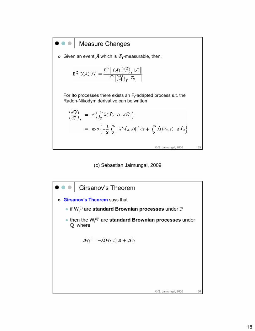
Measure Changes
Given an event A which is FT-measurable, then,
For Ito processes there exists an Ft-adapted process s.t. the Radon-Nikodym derivative can be written
© S. Jaimungal, 2006 36
Girsanov’s Theorem
Girsanov’s Theorem says that
if Wt(i) are standard Brownian processes under P
then the Wt(i)* are standard Brownian processes under
Q where
(c) Sebastian Jaimungal, 2009