Stochastic Calculus

Financial Derivatives

and PDE’s

Simone Calogero

March 18, 2019

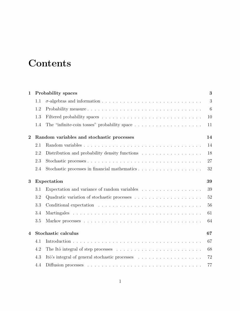
Contents

1 Probability spaces 3

1.1 σ-algebras and information . . . . . . . . . . . . . . . . . . . . . . . . . . . . 3

1.2 Probability measure . . . . . . . . . . . . . . . . . . . . . . . . . . . . . . . . 6

1.3 Filtered probability spaces . . . . . . . . . . . . . . . . . . . . . . . . . . . . 10

1.4 The “infinite-coin tosses” probability space . . . . . . . . . . . . . . . . . . . 11

2 Random variables and stochastic processes 14

2.1 Random variables . . . . . . . . . . . . . . . . . . . . . . . . . . . . . . . . . 14

2.2 Distribution and probability density functions . . . . . . . . . . . . . . . . . 18

2.3 Stochastic processes . . . . . . . . . . . . . . . . . . . . . . . . . . . . . . . . 27

2.4 Stochastic processes in financial mathematics . . . . . . . . . . . . . . . . . . 32

3 Expectation 39

3.1 Expectation and variance of random variables . . . . . . . . . . . . . . . . . 39

3.2 Quadratic variation of stochastic processes . . . . . . . . . . . . . . . . . . . 52

3.3 Conditional expectation . . . . . . . . . . . . . . . . . . . . . . . . . . . . . 56

3.4 Martingales . . . . . . . . . . . . . . . . . . . . . . . . . . . . . . . . . . . . 61

3.5 Markov processes . . . . . . . . . . . . . . . . . . . . . . . . . . . . . . . . . 64

4 Stochastic calculus 67

4.1 Introduction . . . . . . . . . . . . . . . . . . . . . . . . . . . . . . . . . . . . 67

4.2 The Ito integral of step processes . . . . . . . . . . . . . . . . . . . . . . . . 68

4.3 Ito’s integral of general stochastic processes . . . . . . . . . . . . . . . . . . 72

4.4 Diffusion processes . . . . . . . . . . . . . . . . . . . . . . . . . . . . . . . . 77

1

4.5 Girsanov’s theorem . . . . . . . . . . . . . . . . . . . . . . . . . . . . . . . . 82

4.6 Diffusion processes in financial mathematics . . . . . . . . . . . . . . . . . . 84

5 Stochastic differential equations and partial differential equations 88

5.1 Stochastic differential equations . . . . . . . . . . . . . . . . . . . . . . . . . 89

5.2 Kolmogorov equations . . . . . . . . . . . . . . . . . . . . . . . . . . . . . . 92

5.3 The CIR process . . . . . . . . . . . . . . . . . . . . . . . . . . . . . . . . . 96

5.4 Finite different solutions of PDE’s . . . . . . . . . . . . . . . . . . . . . . . . 100

6 Applications to finance 110

6.1 Arbitrage-free markets . . . . . . . . . . . . . . . . . . . . . . . . . . . . . . 110

6.2 The risk-neutral pricing formula . . . . . . . . . . . . . . . . . . . . . . . . . 112

6.3 Black-Scholes price of standard European derivatives . . . . . . . . . . . . . 117

6.4 The Asian option . . . . . . . . . . . . . . . . . . . . . . . . . . . . . . . . . 128

6.5 Local and Stochastic volatility models . . . . . . . . . . . . . . . . . . . . . . 134

6.6 Interest rate contracts . . . . . . . . . . . . . . . . . . . . . . . . . . . . . . 143

6.7 Forwards and Futures . . . . . . . . . . . . . . . . . . . . . . . . . . . . . . . 155

6.8 Multi-dimensional markets . . . . . . . . . . . . . . . . . . . . . . . . . . . . 163

6.9 Introduction to American derivatives . . . . . . . . . . . . . . . . . . . . . . 174

A Numerical projects 183

A.1 A project on the Asian option . . . . . . . . . . . . . . . . . . . . . . . . . . 183

A.2 A project on the CEV model . . . . . . . . . . . . . . . . . . . . . . . . . . . 184

A.3 A project on interest rate models . . . . . . . . . . . . . . . . . . . . . . . . 185

B Solutions to selected problems 187

2

Chapter 1

Probability spaces

1.1 σ-algebras and information

We begin with some notation and terminology. The symbol Ω denotes a generic non-emptyset; the power of Ω, denoted by 2Ω, is the set of all subsets of Ω. If the number of elementsin the set Ω is M ∈ N, we say that Ω is finite. If Ω contains an infinite number of elementsand there exists a bijection Ω↔ N, we say that Ω is countably infinite. If Ω is neither finitenor countably infinite, we say that it is uncountable. An example of uncountable set is theset R of real numbers. When Ω is finite we write Ω = ω1, ω2, . . . , ωM, or Ω = ωkk=1,...,M .If Ω is countably infinite we write Ω = ωkk∈N. Note that for a finite set Ω with M elements,the power set contains 2M elements. For instance, if Ω = ♥, 1, $, then

2Ω = ∅, ♥, 1, $, ♥, 1, ♥, $, 1, $, ♥, 1, $ = Ω,

which contains 23 = 8 elements. Here ∅ denotes the empty set, which by definition is asubset of all sets.

Within the applications in probability theory, the elements ω ∈ Ω are called sample pointsand represent the possible outcomes of a given experiment (or trial), while the subsets of Ωcorrespond to events which may occur in the experiment. For instance, if the experimentconsists in throwing a dice, then Ω = 1, 2, 3, 4, 5, 6 and A = 2, 4, 6 identifies the eventthat the result of the experiment is an even number. Now let Ω = ΩN ,

ΩN = (γ1, . . . , γN), γk ∈ H,T = H,TN ,

where H stands for “head” and T stands for “tail”. Each element ω = (γ1, . . . , γN) ∈ ΩN

is called a N-toss and represents a possible outcome for the experiment “tossing a coin Nconsecutive times”. Evidently, ΩN contains 2N elements and so 2ΩN contains 22N elements.We show in Section 1.4 that Ω∞—the sample space for the experiment “tossing a coininfinitely many times”—is uncountable.

A collection of events, e.g., A1, A2, . . . ⊂ 2Ω, is also called information. The power set

3

of the sample space provides the total accessible information and represents the collection ofall the events that can be resolved (i.e., whose occurrence can be inferred) by knowing theoutcome of the experiment. For an uncountable sample space, the total accessible informa-tion is huge and it is typically replaced by a subclass of events F ⊂ 2Ω, which is imposed toform a σ-algebra.

Definition 1.1. A collection F ⊆ 2Ω of subsets of Ω is called a σ-algebra (or σ-field) onΩ if

(i) ∅ ∈ F ;

(ii) A ∈ F ⇒ Ac := ω ∈ Ω : ω /∈ A ∈ F ;

(iii)⋃∞k=1 Ak ∈ F , for all Akk∈N ⊆ F .

If G is another σ-algebra on Ω and G ⊂ F , we say that G is a sub-σ-algebra of F .

Exercise 1.1. Let F be a σ-algebra. Show that Ω ∈ F and that ∩k∈NAk ∈ F , for allcountable families Akk∈N ⊂ F of events.

Exercise 1.2. Let Ω = 1, 2, 3, 4, 5, 6 be the sample space of a dice roll. Which of thefollowing sets of events are σ-algebras on Ω?

1. ∅, 1, 2, 3, 4, 5, 6,Ω,

2. ∅, 1, 2, 1, 2, 1, 3, 4, 5, 6, 2, 3, 4, 5, 6, 3, 4, 5, 6,Ω,

3. ∅, 2, 1, 3, 4, 5, 6,Ω.Exercise 1.3 (Sol. 1). Prove that the intersection of any number of σ-algebras (includinguncountably many) is a σ-algebra. Show with a counterexample that the union of two σ-algebras is not necessarily a σ-algebra.

Remark 1.1 (Notation). The letter A is used to denote a generic event in the σ-algebra.If we need to consider two such events, we denote them by A,B, while N generic events aredenoted A1, . . . , AN .

Let us comment on Definition 1.1. The empty set represents the “nothing happens” event,while Ac represents the “A does not occur” event. Given a finite number A1, . . . , AN ofevents, their union is the event that at least one of the events A1, . . . , AN occurs, while theirintersection is the event that all events A1, . . . , AN occur. The reason to include the countableunion/intersection of events in our analysis is to make it possible to “take limits” withoutcrossing the boundaries of the theory. Of course, unions and intersections of infinitely manysets only matter when Ω is not finite.

The smallest σ-algebra on Ω is F = ∅,Ω, which is called the trivial σ-algebra. Thereis no relevant information contained in the trivial σ-algebra. The largest possible σ-algebra

4

is F = 2Ω, which contains the full amount of accessible information. When Ω is countable,it is common to pick 2Ω as σ-algebra of events. However, as already mentioned, when Ωis uncountable this choice is unwise. A useful procedure to construct a σ-algebra of eventswhen Ω is uncountable is the following. First we select a collection of events (i.e., subsets ofΩ), which for some reason we regard as fundamental. Let O denote this collection of events.Then we introduce the smallest σ-algebra containing O, which is formally defined as follows.

Definition 1.2. Let O ⊂ 2Ω. The σ-algebra generated by O is

FO =⋂F : F ⊂ 2Ω is a σ-algebra and O ⊆ F

,

i.e., FO is the smallest σ-algebra on Ω containing O.

Recall that the intersection of any number of σ-algebras is still a σ-algebra, see Exercise 1.3,hence FO is a well-defined σ-algebra. For example, let Ω = Rd and let O be the collectionof all open balls:

O = Bx(R)R>0,x∈Rd , where Bx(R) = y ∈ Rd : |x− y| < R.The σ-algebra generated by O is called Borel σ-algebra and denoted B(Rd). The elementsof B(Rd) are called Borel sets.

Remark 1.2 (Notation). The Borel σ-algebra B(R) plays an important role in these notes,so we shall use a specific notation for its elements. A generic event in the σ-algebra B(R)will be denoted U ; if we need to consider two such events we denote them by U, V , while Ngeneric Borel sets of R will be denoted U1, . . . UN . Recall that for general σ-algebras we usethe notation indicated in Remark 1.1.

The σ-algebra generated by O has a particular simple form when O is a partition of Ω.

Definition 1.3. Let I ⊆ N. A collection O = Akk∈I of non-empty subsets of Ω is calleda partition of Ω if

(i) the events Akk∈I are disjoint, i.e., Aj ∩ Ak = ∅, for j 6= k;

(ii)⋃k∈I Ak = Ω.

If I is a finite set we call O a finite partition of Ω.

For example any countable sample space Ω = ωkk∈N is partitioned by the atomic eventsAk = ωk, where ωk identifies the event that the result of the experiment is exactly ωk.

Exercise 1.4. Show that when O is a partition of Ω, the σ-algebra generated by O is givenby the set of all subsets of Ω which can be written as the union of sets in the partition O(plus the empty set, of course).

Exercise 1.5. Find the partition of Ω = 1, 2, 3, 4, 5, 6 that generates the σ-algebra 2 inExercise 1.2.

5

1.2 Probability measure

To any event A ∈ F we want to assign a probability that A occurred.

Definition 1.4. Let F be a σ-algebra on Ω. A probability measure is a function

P : F → [0, 1]

such that

(i) P(Ω) = 1;

(ii) for any countable collection of disjoint events Akk∈N ⊆ F , we have

P

(∞⋃k=1

Ak

)=∞∑k=1

P(Ak).

A triple (Ω,F ,P) is called a probability space.

The quantity P(A) is called probability of the event A; if P(A) = 1 we say that the eventA occurs almost surely, which is sometimes shortened by a.s.; if P(A) = 0 we say thatA is a null set. In general, the elements of F with probability zero or one will be calledtrivial events (as trivial is the information that they provide). For instance, P(Ω) = 1, i.e.,the probability that “something happens” is one, and P(∅) = P(Ωc) = 1−P(Ω) = 0, i.e., theprobability the “nothing happens” is zero.

Exercise 1.6 (Sol. 2). Prove the following properties:

1. P(Ac) = 1− P(A);

2. P(A ∪B) = P(A) + P(B)− P(A ∩B);

3. If A ⊂ B, then P(A) < P(B).

Exercise 1.7 (Continuity of probability measures (?)). Let Akk∈N ⊆ F such that Ak ⊆Ak+1, for all k ∈ N. Let A = ∪kAk. Show that

limk→∞

P(Ak) = P(A).

Similarly, if now Akk∈N ⊆ F such that Ak+1 ⊆ Ak, for all k ∈ N and A = ∩kAk, showthat

limk→∞

P(Ak) = P(A).

Let us see some examples of probability space.

6

• There is only one probability measure defined on the trivial σ-algebra, namely P(∅) = 0and P(Ω) = 1.

• In this example we describe the general procedure to construct a probability space ona countable sample space Ω = ωkk∈N. We pick F = 2Ω and let 0 < pk < 1, k ∈ N,be real numbers such that

∞∑k=1

pk = 1.

We introduce a probability measure on F by first defining the probability of the atomicevents ω1, ω2, . . . as

P(ωk) = pk, k ∈ N.Since every (non-empty) subset of Ω can be written as the disjoint union of atomicevents, then the probability of any event can be inferred using the property (ii) in thedefinition of probability measure, e.g.,

P(ω1, ω3, ω5) = P(ω1 ∪ ω3 ∪ ω5)= P(ω1) + P(ω3) + P(ω5) = p1 + p3 + p5.

In general we define

P(A) =∑

k:ωk∈A

pk, A ∈ 2Ω,

while P(∅) = 0. Note that in countable sample spaces the empty set is the only eventwith zero probability.

• As a special case of the previous example we now introduce a probability measure onthe sample space ΩN of the N -coin tosses experiment. Given 0 < p < 1 and ω ∈ ΩN ,we define the probability of the atomic event ω as

P(ω) = pNH(ω)(1− p)NT (ω), (1.1)

where NH(ω) is the number of H in ω and NT (ω) is the number of T in ω (NH(ω) +NT (ω) = N). We say that the coin is fair if p = 1/2. The probability of a genericevent A ∈ F = 2ΩN is obtained by adding up the probabilities of the atomic eventswhose disjoint union forms the event A. For instance, assume N = 3 and consider theevent

“The first and the second toss are equal”.

Denote by A ∈ F the set corresponding to this event. Then clearly A is the (disjoint)union of the atomic events

(H,H,H), (H,H, T ), (T, T, T ), (T, T,H).Hence,

P(A) = P((H,H,H)) + P((H,H, T )) + P((T, T, T )) + P((T, T,H))= p3 + p2(1− p) + (1− p)3 + (1− p)2p = 2p2 − 2p+ 1.

7

In Section 1.4 it is shown how to extend the probability measure (1.1) to Ω∞ usingCaratheodory’s theorem.

• Let f : R→ [0,∞) be a measurable function1 such that∫Rf(x) dx = 1.

Then

P(U) =

∫U

f(x) dx, (1.2)

defines a probability measure on B(R).

Remark 1.3 (Riemann vs. Lebesgue integral). The integral in (1.2) must be understoodin the Lebesgue sense, since we are integrating a general measurable function over a generalBorel set. If f is sufficiently regular (say, continuous), and U = (a, b) ⊂ R is an interval, thenthe integral in (1.2) can be understood in the Riemann sense. Although the latter case isoften sufficient in many applications (including in finance), all integrals in these notes shouldbe understood in the Lebesgue sense, unless otherwise stated. The knowledge of Lebesgueintegration theory is however not required for our purposes.

Exercise 1.8 (Sol. 3). Prove that∑

ω∈ΩNP(ω) = 1, where P(ω) is given by (1.1).

Equivalent probability measures

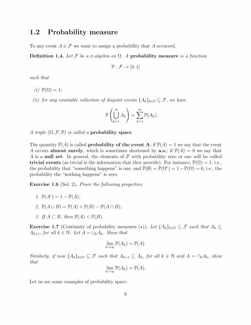
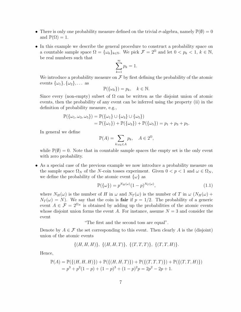
A probability space is a triple (Ω,F ,P) and if we change one element of this triple we get adifferent probability space. The most interesting case is when a new probability measure isintroduced. Let us first show with an example (known as Bertrand’s paradox) that theremight not be just one “reasonable” definition of probability measure associated to a givenexperiment. Suppose we perform an experiment whose result is a pair of points p, q on theunit circle C (e.g., throw two balls in a roulette). The sample space for this experiment isΩ = (p, q) : p, q ∈ C. Let T be the length of the chord joining p and q. Now let L bethe length of the side of a equilateral triangle inscribed in the circle C. Note that all suchtriangles are obtained one from another by a rotation around the center of the circle andall have the same sides length L. Consider the event A = (p, q) ∈ Ω : T > L. Whatis a reasonable definition for P(A)? From one hand we can suppose that one vertex of thetriangle is p, and thus T will be greater than L if and only if the point q lies on the archof the circle between the two vertexes of the triangle different from p, see Figure 1.1(a).Since the length of such arc is 1/3 the perimeter of the circle, then it is reasonable to defineP(A) = 1/3. On the other hand, it is simple to see that T > L whenever the midpoint m ofthe chord lies within a circle of radius 1/2 concentric to C, see Figure 1.1(b). Since the areaof the interior circle is 1/4 the area of C, we are led to define P(A) = 1/4.

1See Section 2.1 for the definition of measurable function.

8

p

q

L

T

(a) P(A) = 1/3

p

qL

1/2 m

(b) P(A) = 1/4

Figure 1.1: The Bertrand paradox. The length T of the cord pq is greater then L.

Whenever two probabilities are defined for the same experiment, it is of particular interestto determine whether they are equivalent, in the following sense.

Definition 1.5. Given two probability spaces (Ω,F ,P) and (Ω,F , P), the probability mea-

sures P and P are said to be equivalent if P(A) = 0⇔ P(A) = 0.

Hence equivalent probability measures agree on which events are impossible. A completecharacterization of the probability measures P equivalent to a given P will be given in The-orem 3.3.

Conditional probability. Independent events

It might be that the occurrence of an event B makes the occurrence of another event A moreor less likely. For instance, the probability of the event A = the first two tosses of a faircoin are both head is 1/4; however if know that the first toss is a tail, then P(A) = 0, whileP(A) = 1/2 if we know that the first toss is a head. This leads to the important definitionof conditional probability.

Definition 1.6. Given two events A,B such that P(B) > 0, the conditional probabilityof A given B is defined as

P(A|B) =P(A ∩B)

P(B).

To justify this definition, let FB = A ∩BA∈F , and set

PB(·) = P(·|B).

9

Then (B,FB,PB) is a probability space in which the events that cannot occur simultaneouslywith B are null events. Therefore it is natural to regard (B,FB,PB) as the restriction of theprobability space (Ω,F ,P) when B has occurred.

If P(A|B) = P(A), the two events are said to be independent. The interpretation is thefollowing: if two events A,B are independent, then the occurrence of the event B does notchange the probability that A occurred. By Definition 1.6 we obtain the following equivalentcharacterization of independent events.

Definition 1.7. Two events A,B are said to be independent if P(A∩B) = P(A)P(B). Ingeneral, the events A1, . . . , AN (N ≥ 2) are said to be independent if, for all 1 ≤ k1 < k2 <· · · < km ≤ N , we have

P(Ak1 ∩ · · · ∩ Akm) =m∏j=1

P(Akj).

Two σ-algebras F ,G are said to be independent if A and B are independent, for all A ∈ Gand B ∈ F . In general the σ-algebras F1, . . . ,FN (N ≥ 2) are said to be independent ifA1, A2, . . . , AN are independent events, for all A1 ∈ F1, . . . , AN ∈ FN .

Note carefully that the independence property of events is connected to the probabilitymeasure, i.e., two events may be independent in the probability P and not independent inthe probability P, even if P and P are equivalent. Note also that if F ,G are two independentσ-algebras and A ∈ F ∩ G, then A is a trivial event. In fact, if A ∈ F ∩ G, then P(A) =P(A ∩ A) = P(A)2. Hence P(A) = 0 or 1. The interpretation of this simple remark is thatindependent σ-algebras carry separate information.

Exercise 1.9 (Sol. 4). Given a fair coin and assuming N is odd, consider the following twoevents A,B ∈ ΩN :

A = “the number of heads is greater than the number of tails”,

B = “The first toss is a head”.

Use your intuition to guess whether the two events are independent; then verify your answernumerically (e.g., using Mathematica).

1.3 Filtered probability spaces

Consider again the N -coin tosses probability space. Let AH be the event that the first toss isa head and AT the event that it is a tail. Clearly AT = AcH and the σ-algebra F1 generatedby the partition AH , AT is F1 = AH , AT ,Ω, ∅. Now let AHH be the event that the first 2tosses are heads, and similarly define AHT , ATH , ATT . These four events form a partition ofΩN and they generate a σ-algebra F2 as indicated in Exercise 1.4. Clearly, F1 ⊂ F2. Going

10

on with three tosses, four tosses, and so on, until we complete the N -toss, we construct asequence

F1 ⊂ F2 ⊂ · · · ⊂ FN = 2ΩN

of σ-algebras. The σ-algebra Fk contains all the events of the experiment that depend on(i.e., which are resolved by) the first k tosses. The family Fkk=1,...,N of σ-algebras is anexample of filtration.

Definition 1.8. A filtration is a one parameter family F(t)t≥0 of σ-algebras such thatF(t) ⊆ F for all t ≥ 0 and F(s) ⊆ F(t) for all s ≤ t. A quadruple (Ω,F , F(t)t≥0,P) iscalled a filtered probability space.

In our applications t stands for the time variable and filtrations are associated to experimentsin which “information accumulates with time”. For instance, in the example given above,the more times we toss the coin, the higher is the number of events which are resolved bythe experiment, i.e., the more information becomes accessible.

1.4 The “infinite-coin tosses” probability space

In this section we outline the construction of the probability space for the ∞-coin tossesexperiment using Caratheodory’s theorem. The sample space is

Ω∞ = ω = (γn)n∈N, γn ∈ H,T.

Let us show first that Ω is uncountable. We use the well-known Cantor diagonal argu-ment. Suppose that Ω∞ is countable and write

Ω∞ = ωkk∈N. (1.3)

Each ωk ∈ Ω∞ is a sequence of infinite tosses, which we write as ωk = (γ(k)j )j∈N, where γ

(k)j

is either H or T , for all j ∈ N and for each fixed k ∈ N. Note that (γ(k)j )j,k∈N is an “∞×∞”

matrix. Now consider the ∞-toss corresponding to the diagonal of this matrix, that is

ω = (γm)m∈N, γm = γ(m)m , for all m ∈ N.

Finally consider the∞-toss ω which is obtained by changing each single toss of ω, that is tosay

ω = (γm)m∈N, where γm = H if γm = T , and γm = T if γm = H, for all m ∈ N.

It is clear that the ∞-toss ω does not belong to the set (1.3). In fact, by construction, thefirst toss of ω is different from the first toss of ω1, the second toss of ω is different from thesecond toss of ω2, . . . , the nth toss of ω is different from the nth toss of ωn, and so on, so

11

that each ∞-toss in (1.3) is different from ω. We conclude that the elements of Ω∞ cannotbe listed as they were comprising a countable set.

Now, let N ∈ N and ΩN = H,TN be the sample space for the N -tosses experiment. Foreach ω = (γ1, . . . , γN) ∈ ΩN we define the event Aω ⊂ Ω∞ by

Aω = ω = (γn)n∈N : γj = γj, j = 1, . . . , N,i.e., the event that the first N tosses in a ∞-toss be equal to (γ1, . . . , γN). Define theprobability of this event as the probability of the N -toss ω, that is

P0(Aω) = pNH(ω)(1− p)NT (ω),

where 0 < p < 1, NH(ω) is the number of heads in the N -toss ω and NT (ω) = N −NH(ω)is the number of tails in ω, see (1.1). Next consider the family of events

UN = Aωω∈ΩN ⊂ 2Ω∞ .

It is clear that UN is, for each fixed N ∈ N, a partition of Ω∞. Hence the σ-algebraFN = FUN is generated according to Exercise 1.4. Note that FN contains all events of Ω∞that are resolved by the first N tosses. Moreover FN ⊂ FN+1, that is to say, FNN∈N isa filtration. Since P0 is defined for all Aω ∈ UN , then it can be extended uniquely to theentire FN , because each element A ∈ FN is the disjoint union of events of UN (see againExercise 1.4) and therefore the probability of A can be inferred by the property (ii) in thedefinition of probability measure, see Definition 1.4. But then P0 extends uniquely to

F∞ =⋃N∈N

FN .

Hence we have constructed a triple (Ω∞,F∞,P0). Is this triple a probability space? Theanswer is no, because F∞ is not a σ-algebra. To see this, let Ak be the event that thekth toss in a infinite sequence of tosses is a head. Clearly Ak ∈ Fk for all k and thereforeAkk∈N ⊂ F∞. Now assume that F∞ is a σ-algebra. Then the event A = ∪kAk wouldbelong to F∞ and therefore also Ac ∈ F∞. The latter holds if and only if there exists N ∈ Nsuch that Ac ∈ FN . But Ac is the event that all tosses are tails, which of course cannot beresolved by the information FN accumulated after just N tosses. We conclude that F∞ isnot a σ-algebra. In particular, we have shown that F∞ is not in general closed with respectto the countable union of its elements. However it is easy to show that F∞ is closed withrespect to the finite union of its elements, and in addition satisfies the properties (i), (ii) inDefinition 1.4. This set of properties makes F∞ an algebra. To complete the constructionof the probability space for the∞-coin tosses experiment, we need the following deep result.

Theorem 1.1 (Caratheodory’s theorem). Let U be an algebra of subsets of Ω and P0 :U → [0, 1] a map satisfying P0(Ω) = 1 and P0(∪Ni=1Ai) =

∑Ni=1 P0(Ai), for every finite

collection A1, . . . , AN ⊂ U of disjoint sets2. Then there exists a unique probability measureP on FU such that P(A) = P0(A), for all A ∈ U .

2P0 is called a pre-measure.

12

Hence the map P0 : F∞ → [0, 1] defined above extends uniquely to a probability measure Pdefined on F = FF∞ . The resulting triple (Ω∞,F ,P) defines the probability space for the∞- coin tosses experiment.

13

Chapter 2

Random variables and stochasticprocesses

Throughout this chapter we assume that (Ω,F , F(t)t≥0,P) is a given filtered probabilityspace.

2.1 Random variables

In many applications of probability theory, and in financial mathematics in particular, oneis more interested in knowing the value attained by quantities that depend on the outcomeof the experiment, rather than knowing which specific events have occurred. Such quantitiesare called random variables.

Definition 2.1. A map X : Ω → R is called a (real-valued) random variable if X ∈U ∈ F , for all U ∈ B(R), where X ∈ U = ω ∈ Ω : X(ω) ∈ U is the pre-image of theBorel set U . If there exists c ∈ R such that X(ω) = c almost surely, we say that X is adeterministic constant.

Occasionally we shall also need to consider complex-valued random variables. These aredefined as the maps Z : Ω→ C of the form Z = X+ iY , where X, Y are real-valued randomvariables and i is the imaginary unit (i2 = −1). Similarly a vector valued random variableX = (X1, . . . , XN) : Ω → RN can be defined by simply requiring that each componentXj : Ω→ R is a random variable in the sense of Definition 2.1.

Remark 2.1 (Notation). A generic real-valued random variable will be denoted by X. Ifwe need to consider two such random variables we will denote them by X, Y , while N real-valued random variables will be denoted by X1, . . . , XN . Note that (X1, . . . , XN) : Ω→ RN

is a vector-valued random variable.

Remark 2.2. Equality among random variables is always understood to hold up to a nullset. That is to say, X = Y always means X = Y almost surely (a.s.).

14

Random variables are also called measurable functions, but this terminology will be usedin this text only when Ω = R and F = B(R). Measurable functions will be denoted by smallLatin letters (e.g., f, g, . . . ). If X is a random variable and Y = f(X) for some measurablefunction f , then Y is also a random variable. We denote P(X ∈ U) = P(X ∈ U)the probability that X takes value in U ∈ B(R). Moreover, given two random variablesX, Y : Ω→ R and the Borel sets U, V , we denote

P(X ∈ U, Y ∈ V ) = P(X ∈ U ∩ Y ∈ V ),which is the probability that the random variable X takes value in U and Y takes value inV . The generalization to an arbitrary number of random variables is straightforward.

As the value attained by X depends on the result of the experiment, random variables carryinformation, i.e., upon knowing the value attained by X we know something about theoutcome ω of the experiment. For instance, if X(ω) = (−1)ω, where ω is the result of tossinga dice, and if we are told that X takes value 1, then we infer immediately that the dice rollis even. The information carried by a random variable X forms the σ-algebra generated byX, whose precise definition is the following.

Definition 2.2. Let X : Ω→ R be a random variable. The σ-algebra generated by X isthe collection σ(X) ⊆ F of events given by

σ(X) = A ∈ F : A = X ∈ U, for some U ∈ B(R).If G ⊆ F is another σ-algebra of subsets of Ω and σ(X) ⊆ G, we say that X is G-measurable. If Y : Ω → R is another random variable and σ(Y ) ⊆ σ(X), we say thatY is X-measurable

Exercise 2.1 (Sol. 5). Prove that σ(X) is a σ-algebra.

Thus σ(X) contains all the events that are resolved by knowing the value of X. The in-terpretation of X being G-measurable is that the information contained in G suffices todetermine the value taken by X in the experiment. Note that the σ-algebra generated by adeterministic constant consists of trivial events only.

Definition 2.3. The σ-algebra σ(X, Y ) generated by two random variables X, Y : Ω → Ris the smallest σ-algebra containing σ(X) ∪ σ(Y ), that is to say1 σ(X, Y ) = FO, whereO = σ(X) ∪ σ(Y ), and similarly for any number of random variables.

If Y is X-measurable then σ(X, Y ) = σ(X), i.e., the random variable Y does not addany new information to the one already contained in X. Clearly, if Y = f(X) for somemeasurable function f , then Y is X-measurable. It can be shown that the opposite is alsotrue: if σ(Y ) ⊆ σ(X), then there exists a measurable function f such that Y = f(X) (seeProp. 3 in [22]). The other extreme is when X and Y carry distinct information, i.e., whenσ(X) ∩ σ(Y ) consists of trivial events only. This occurs in particular when the two randomvariables are independent.

1See Definition 1.2.

15

Definition 2.4. Let X : Ω → R be a random variable and G ⊂ F be a sub-σ-algebra. Wesay that X is independent of G if σ(X) and G are independent in the sense of Definition 1.7.Two random variables X, Y : Ω → R are said to be independent random variablesif the σ-algebras σ(X) and σ(Y ) are independent. More generally, the random variablesX1, . . . , XN are independent if σ(X1), . . . , σ(XN) are independent σ-algebras.

In the intermediate case, i.e., when Y is neither X-measurable nor independent of X, it isexpected that the knowledge on the value attained by X helps to derive information on thevalues attainable by Y . We shall study this case in the next chapter.

Exercise 2.2 (Sol. 6). Show that when X, Y are independent random variables, then σ(X)∩σ(Y ) consists of trivial events only (i.e., events with probability zero or one). Show that twodeterministic constants are always independent. Finally assume Y = g(X) and show thatin this case the two random variables are independent if and only if Y is a deterministicconstant.

Exercise 2.3. Which of the following pairs of random variables X, Y : ΩN → R are indepen-dent? (Use only the intuitive interpretation of independence and not the formal definition.)

1. X(ω) = NT (ω); Y (ω) = 1 if the first toss is head, Y (ω) = 0 otherwise.

2. X(ω) = 1 if there exists at least a head in ω, X(ω) = 0 otherwise; Y (ω) = 1 if thereexists exactly a head in ω, Y (ω) = 0 otherwise.

3. X(ω) = number of times that a head is followed by a tail; Y (ω) = 1 if there exist twoconsecutive tail in ω, Y (ω) = 0 otherwise.

The next theorem shows how to construct new independent random variables from a givensequence of independent random variables.

Theorem 2.1. Let X1, . . . , XN be independent random variables. Let us divide the setX1, . . . , XN into m separate groups of random variables, namely, let

X1, . . . , XN = Xk1k1∈I1 ∪ Xk2k2∈I2 ∪ · · · ∪ Xkmkm∈Im ,where I1, I2, . . . Im is a partition of 1, . . . , N. Let ni be the number of elements in theset Ii, so that n1 + n2 + · · · + nm = N . Let g1, . . . , gm be measurable functions such thatgi : Rni → R. Then the random variables

Y1 = g1((Xk1)k1∈I1), Y2 = g2((Xk2)k2∈I2), . . . , Ym = gm((Xkm)km∈Im)

are independent.

For instance, in the case of N = 2 independent random variables X1, X2, Theorem 2.1 assertsthat Y1 = g(X1) and Y2 = f(X2) are independent random variables, for all measurablefunctions f, g : R→ R.

Exercise 2.4 (Sol. 7). Prove Theorem 2.1 for the case N = 2.

16

Simple and discrete Random Variables

A special role is played by simple random variables. The simplest possible one is the indica-tor function of an event: Given A ∈ F , the indicator function of A is the random variablethat takes value 1 if ω ∈ A and 0 otherwise, i.e.,

IA(ω) =

1, ω ∈ A,0, ω ∈ Ac.

Obviously, σ(IA) = A,Ac, ∅,Ω.Definition 2.5. Let Akk=1....,N ⊂ F be a finite partition of Ω and a1, . . . , aN be distinctreal numbers. The random variable

X =N∑k=1

akIAk

is called a simple random variable. If N = ∞ in this definition, we call X a discreterandom variable.

Thus a simple random variable X attains only a finite number of values, while a discreterandom variable X attains countably infinite many values2. In both cases we have

P(X = x) =

0, if x /∈ Image(X),P(Ak), if x = ak,

where Image(X) = x ∈ R : X(ω) = x, for some ω ∈ Ω is the image of X. Moreover fora simple, or discrete, random variable X, σ(X) is the σ-algebra generated by the partitionA1, A2, . . . , which is constructed as stated in Exercise 1.4. Let us consider two examplesof simple/discrete random variables that have applications in financial mathematics (and inmany other fields).

A simple random variable X is called a binomial random variable if

• Image(X) = 0, 1, . . . , N;

• There exists p ∈ (0, 1) such that P(X = k) =(Nk

)pk(1− p)N−k, k = 0, . . . , N .

For instance, if we let X to be the number of heads in a N -toss, then X is binomial.

A discrete random variable X is called a Poisson variable if

• Image(X) = N ∪ 0;

• There exists µ > 0 such that P(X = k) =µke−µ

k!, k = 0, 1, 2, . . .

2Not all authors distinguish between simple and discrete random variables.

17

We denote by P(µ) the set of all Poisson random variables with parameter µ > 0.

The following important theorem shows that all non-negative random variables can be ap-proximated by a sequence of simple random variables.

Theorem 2.2. Let X : Ω → [0,∞) be a random variable and let n ∈ N be given. Fork = 0, 1, ...n2n − 1, consider the sets

Ak,n :=X ∈

[ k2n,k + 1

2n

)and for k = n2n let

An2n,n = X ≥ n.Note that Ak,nk=0,...,n2n is a partition of Ω, for all fixed n ∈ N. Define the simple randomvariables

sXn (ω) =n2n∑k=0

k

2nIAk,n(ω).

Then 0 ≤ sX1 (ω) ≤ sX2 (ω) ≤ · · · ≤ sXn (ω) ≤ sXn+1(ω) ≤ · · · ≤ X(ω), for all ω ∈ Ω (i.e., thesequence sXn n∈N is non-decreasing) and

limn→∞

sXn (ω) = X(ω), for all ω ∈ Ω.

Exercise 2.5. Prove Theorem 2.2.

2.2 Distribution and probability density functions

Definition 2.6. The (cumulative) distribution function of the random variable X :Ω → R is the non-negative function FX : R → [0, 1] given by FX(x) = P(X ≤ x). Tworandom variables X, Y are said to be identically distributed if FX = FY .

Exercise 2.6 (Sol. 8). Show that

P(a < X ≤ b) = FX(b)− FX(a).

Show also that FX is (1) right-continuous, (2) non-decreasing, (3) limx→+∞ FX(x) = 1 andlimx→−∞ FX(x) = 0.

Exercise 2.7 (Sol. 9). Let F : R→ [0, 1] be a measurable function satisfying the properties(1)–(3) in Exercise 2.6. Show that there exists a probability space and a random variable Xsuch that F = FX .

Definition 2.7. A random variable X : Ω → R is said to admit the probability densityfunction (pdf) fX : R→ [0,∞) if fX is integrable on R and

FX(x) =

∫ x

−∞fX(y) dy. (2.1)

18

Note that if fX is the pdf of a random variable, then necessarily∫RfX(x) dx = lim

x→∞FX(x) = 1.

All probability density functions considered in these notes are almost everywhere continuous3,and therefore the integral in (2.1) can be understood in the Riemann sense. Moreover inthis case FX is differentiable and we have

fX =dFXdx

.

If the integral in (2.1) is understood in the Lebesgue sense, then the density fX can be aquite irregular function. In this case, the fundamental theorem of calculus for the Lebesgueintegral entails that the distribution FX(x) satisfying (2.1) is absolutely continuous, and soin particular it is continuous. Conversely, if FX is absolutely continuous, then X admits adensity function.

We remark that, regardless of the notion of integral being used, a simple (or discrete) randomvariable X cannot admit a density in the sense of Definition 2.7. Suppose in fact thatX =

∑Nk=1 akIAk is a simple random variable and assume a1 = max(a1, . . . , aN). Then

limx→a−1

FX(x) = P(A2) + · · ·+ P(AN) < 1,

whilelimx→a+

1

FX(x) = 1 = FX(a1).

It follows that FX(x) is not continuous, and so in particular it cannot be written in theform (2.1). To define the pdf of the simple random variable X =

∑Nk=1 akIAk , we observe

first that its distribution function is

FX(x) = P(X ≤ x) =∑ak≤x

P(X = ak). (2.2)

The probability density function fX(x) is defined as

fX(x) =

P(X = x), if x = ak for some k

0 otherwise.

Thus with a slight abuse of notation we can rewrite (2.2) as

FX(x) =∑y≤x

fX(y), (2.3)

3I.e., continuous everywhere except possibly in a real set of zero Lebesgue measure.

19

which extends (2.1) to simple random variables4.

We shall see in the following chapters that if a random variable X admits a density, then allthe relevant statistical information on X can be deduced by fX . We also remark that oftenone can prove the existence of the pdf fX without however being able to derive an explicitformula for it. For instance, fX is often given as the solution of a partial differential equation,or through its (inverse) Fourier transform, which is called the characteristic function of X,see Section 3.1. Some examples of density functions, which have important applications infinancial mathematics, are the following.

Examples of probability density functions

• A random variable X : Ω → R is said to be a normal (or normally distributed)random variable if it admits the density

fX(x) =1√

2πσ2e−

(x−m)2

2σ2 ,

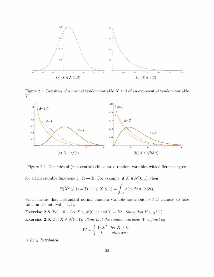
for some m ∈ R and σ > 0, which are called respectively the expectation (or mean)and the deviation of the normal random variable X, while σ2 is called the varianceof X. The typical profile of a normal density function is shown in Figure 2.1(a). Wedenote by N (m,σ2) the set of all normal random variables with expectation m andvariance σ2. If m = 0 and σ2 = 1, X ∈ N (0, 1) is said to be a standard normalvariable. The density function of standard normal random variables is denoted by φ,while their distribution is denoted by Φ, i.e.,

φ(x) =1√2πe−

x2

2 , Φ(x) =1√2π

∫ x

−∞e−

y2

2 dy.

• A random variable X : Ω → R is said to be an exponential (or exponentiallydistributed) random variable if it admits the density

fX(x) = λe−λxIx≥0,

for some λ > 0, which is called the intensity of the exponential random variable X. Atypical profile is shown in Figure 2.1(b) . We denote by E(λ) the set of all exponentialrandom variables with intensity λ > 0. The distribution function of an exponentialrandom variable X with intensity λ is given by

FX(x) =

∫ x

−∞fX(y) dy = λ

∫ x

0

e−λy dy = 1− e−λx.

4It is possible to unify the definition of pdf for continuum and discrete random variables by writing thesum (2.3) as an integral with respect to the Dirac measure, but we shall not do so.

20

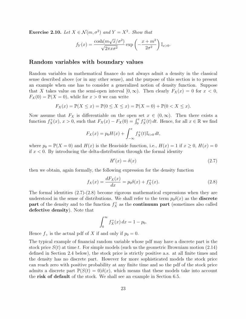
• A random variable X : Ω→ R is said to be chi-squared distributed if it admits thedensity

fX(x) =xδ/2−1e−x/2

2δ/2Γ(δ/2)Ix>0,

for some δ > 0, which is called the degree of X. Here Γ(t) =∫∞

0zt−1e−zdz, t > 0, is

the Gamma-function. Recall the relation

Γ(n) = (n− 1)!

for n ∈ N. We denote by χ2(δ) the set of all chi-squared distributed random variableswith degree δ. Three typical profiles of this density are shown in Figure 2.2(a).

• A random variable X : Ω → R is said to be non-central chi-squared distributedwith degree δ > 0 and non-centrality parameter β > 0 if it admits the density

fX(x) =1

2e−

x+β2

(x

β

) δ4− 1

2

Iδ/2−1(√βx)Ix>0, (2.4)

where Iν(y) denotes the modified Bessel function of the first kind. We denote by χ2(δ, β)the random variables with density (2.4). It can be shown that χ2(δ, 0) = χ2(δ). Threetypical profiles of the density (2.4) are shown in Figure 2.2(b).

• A random variable X : Ω → R is said to be Cauchy distributed if it admits thedensity

fX(x) =γ

π((x− x0)2 + γ2)

for x0 ∈ R and γ > 0 , called the location and the scale of X.

• A random variable X : Ω→ R is said to be Levy distributed if it admits the density

fX(x) =

√c

2π

e− c

2(x−x0)

(x− x0)3/2Ix>x0 ,

for x0 ∈ R and c > 0, called the location and the scale of X.

If a random variable X admits a density fX , then for all (possibly unbounded) intervalsI ⊆ R the result of Exercise 2.6 entails

P(X ∈ I) =

∫I

fX(y) dy. (2.5)

It can be shown that (2.5) extends to

P(g(X) ∈ I) =

∫x:g(x)∈I

fX(x) dx, (2.6)

21

-6 -4 -2 2 4 6 8

0.05

0.10

0.15

0.20

(a) X ∈ N (1, 2)

0.5 1.0 1.5 2.0 2.5 3.0

0.5

1.0

1.5

2.0

(b) X ∈ E(2)

Figure 2.1: Densities of a normal random variable X and of an exponential random variableY .

∆=1/2

∆=1

∆=4

1 2 3 4

0.2

0.4

0.6

0.8

1.0

1.2

(a) X ∈ χ2(δ)

∆=1

∆=2

∆=5

5 10 15 20

0.05

0.10

0.15

0.20

0.25

(b) X ∈ χ2(δ, 2)

Figure 2.2: Densities of (non-central) chi-squared random variables with different degree.

for all measurable functions g : R→ R. For example, if X ∈ N (0, 1), then

P(X2 ≤ 1) = P(−1 ≤ X ≤ 1) =

∫ 1

−1

φ(x) dx ≈ 0.683,

which means that a standard normal random variable has about 68.3 % chances to takevalue in the interval [−1, 1].

Exercise 2.8 (Sol. 10). Let X ∈ N (0, 1) and Y = X2. Show that Y ∈ χ2(1).

Exercise 2.9. Let X ∈ N (0, 1). Show that the random variable W defined by

W =

1/X2 for X 6= 0,

0 otherwise

is Levy distributed.

22

Exercise 2.10. Let X ∈ N (m,σ2) and Y = X2. Show that

fY (x) =cosh(m

√x/σ2)√

2πxσ2exp

(−x+m2

2σ2

)Ix>0.

Random variables with boundary values

Random variables in mathematical finance do not always admit a density in the classicalsense described above (or in any other sense), and the purpose of this section is to presentan example when one has to consider a generalized notion of density function. Supposethat X takes value on the semi-open interval [0,∞). Then clearly FX(x) = 0 for x < 0,FX(0) = P(X = 0), while for x > 0 we can write

FX(x) = P(X ≤ x) = P(0 ≤ X ≤ x) = P(X = 0) + P(0 < X ≤ x).

Now assume that FX is differentiable on the open set x ∈ (0,∞). Then there exists afunction f+

X (x), x > 0, such that FX(x)− FX(0) =∫ x

0f+X (t) dt. Hence, for all x ∈ R we find

FX(x) = p0H(x) +

∫ x

−∞f+X (t)It>0 dt,

where p0 = P(X = 0) and H(x) is the Heaviside function, i.e., H(x) = 1 if x ≥ 0, H(x) = 0if x < 0. By introducing the delta-distribution through the formal identity

H ′(x) = δ(x) (2.7)

then we obtain, again formally, the following expression for the density function

fX(x) =dFX(x)

dx= p0δ(x) + f+

X (x). (2.8)

The formal identities (2.7)-(2.8) become rigorous mathematical expressions when they areunderstood in the sense of distributions. We shall refer to the term p0δ(x) as the discretepart of the density and to the function f+

X as the continuum part (sometimes also calleddefective density). Note that ∫ ∞

0

f+X (x) dx = 1− p0.

Hence f+ is the actual pdf of X if and only if p0 = 0.

The typical example of financial random variable whose pdf may have a discrete part is thestock price S(t) at time t. For simple models (such us the geometric Browniam motion (2.14)defined in Section 2.4 below), the stock price is strictly positive a.s. at all finite times andthe density has no discrete part. However for more sophisticated models the stock pricecan reach zero with positive probability at any finite time and so the pdf of the stock priceadmits a discrete part P(S(t) = 0)δ(x), which means that these models take into accountthe risk of default of the stock. We shall see an example in Section 6.5.

23

Joint distribution

Definition 2.8. The joint (cumulative) distribution FX,Y : R2 → [0, 1] of two randomvariables X, Y : Ω→ R is defined as

FX,Y (x, y) = P(X ≤ x, Y ≤ y).

It can be shown that two random variables are independent if and only if FX,Y (x, y) =FX(x)FY (y). In Theorem 2.3 below we prove a special case of this result assuming that thetwo random variables admit a joint pdf, defined as follows.

Definition 2.9. The random variables X, Y are said to admit the joint (probability)density function fX,Y : R2 → [0,∞) if fX,Y is integrable in R2 and

FX,Y (x, y) =

∫ x

−∞

∫ y

−∞fX,Y (η, ξ) dη dξ.

Note the formal identities

fX,Y =∂2FX,Y∂x ∂y

,

∫R2

fX,Y (x, y) dx dy = 1.

Moreover, if two random variables X, Y admit a joint density fX,Y , then each of them admitsa density (called marginal density in this context) which is given by

fX(x) =

∫RfX,Y (x, y) dy, fY (y) =

∫RfX,Y (x, y) dx.

To see this we write

P(X ≤ x) = P(X ≤ x, Y ∈ R) =

∫ x

−∞

∫RfX,Y (η, ξ) dη dξ =

∫ x

−∞fX(η) dη

and similarly for the random variable Y . If W = g(X, Y ), for some measurable function g,and I ⊆ R is an interval, the analogue of (2.6) in 2 dimensions holds, namely:

P(g(X, Y ) ∈ I) =

∫x,y:g(x,y)∈I

fX,Y (x, y) dx dy.

As an example of joint pdf, let m = (m1 m2) be a two dimensional row vector and C =(Cij)i,j=1,2 be a 2×2 positive definite, symmetric matrix. Two random variables X1, X2 : Ω→R are said to be jointly normally distributed with mean m and covariance matrix Cif they admit the joint density

fX1,X2(x) =1√

(2π)2 detCexp

[−1

2(x−m)C−1(x−m)T

], (2.9)

where x = (x1 x2), C−1 is the inverse matrix of C and vT is the transpose of the vector v. Wedenote by N (m,C) the set of jointly normally distributed random variables X = (X1, X2)with mean m ∈ R2 and covariance matrix C.

24

Exercise 2.11 (Sol. 11). Show that two random variables X1, X2 are jointly normally dis-tributed if and only if

fX1,X2(x) =1

2πσ1σ2

√1− ρ2

×

× exp

(− 1

2(1− ρ2)

[(x1 −m1)2

σ21

− 2ρ(x1 −m1)(x2 −m2)

σ1σ2

+(x2 −m2)2

σ22

]), (2.10)

where

σ21 = C11, σ2

2 = C22, ρ =C12

σ1σ2

.

Moreover show that (X1, X2) ∈ N (m,C) implies X1 ∈ N (m1, σ1), X2 ∈ N (m2, σ2).

By the previous exercise, when σ1 = σ2 = 1 and m = (0 0), each random variable X1, X2 is astandard normal random variable. We denote by φ(x1, x2; ρ) the joint normal density in thiscase and call it the (2-dimensional) standard joint normal density with correlationcoefficient ρ:

φ(x1, x2; ρ) =1

2π√

1− ρ2exp

(−x

21 − 2ρx1x2 + x2

2

2(1− ρ2)

). (2.11)

The corresponding cumulative distribution is given by

Φ(x1, x2; ρ) =

∫ x1

−∞

∫ x2

−∞φ(y1, y2; ρ) dy1 dy2. (2.12)

In the next theorem we establish a simple condition for the independence of two randomvariables which admit a joint density.

Theorem 2.3. The following holds.

(i) If two random variables X, Y admit the densities fX , fY and are independent, thenthey admit the joint density

fX,Y (x, y) = fX(x)fY (y).

(ii) If two random variables X, Y admit a joint density fX,Y of the form

fX,Y (x, y) = u(x)v(y),

for some functions u, v : R→ [0,∞), then X, Y are independent and admit the densi-ties fX , fY given by

fX(x) = cu(x), fY (y) =1

cv(y),

where

c =

∫Rv(x) dx =

(∫Ru(y) dy

)−1

.

25

Proof. As to (i) we have

FX,Y (x, y) = P(X ≤ x, Y ≤ y) = P(X ≤ x)P(Y ≤ y)

=

∫ x

−∞fX(η) dη

∫ y

−∞fY (ξ) dξ

=

∫ x

−∞

∫ y

−∞fX(η)fY (ξ) dη dξ.

To prove (ii), we first write

X ≤ x = X ≤ x ∩ Ω = X ≤ x ∩ Y ≤ R = X ≤ x, Y ≤ R.

Hence,

P(X ≤ x) =

∫ x

−∞

∫ ∞−∞

fX,Y (η, y) dy dη =

∫ x

−∞u(η) dη

∫Rv(y) dy =

∫ x

−∞cu(η) dη,

where c =∫R v(y) dy. Thus X admits the density fX(x) = c u(x). At the same fashion one

proves that Y admits the density fY (y) = c′v(y), where c′ =∫R u(x)dx. Since

1 =

∫R

∫RfX,Y (x, y) dx dy =

∫Ru(x) dx

∫Rv(y) dy = c′c,

then c′ = 1/c. It remains to prove that X, Y are independent. This follows by

P(X ∈ U, Y ∈ V ) =

∫U

∫V

fX,Y (x, y) dx dy =

∫U

u(x) dx

∫V

v(y) dy

=

∫U

cu(x) dx

∫V

1

cv(y) dy =

∫U

fX(x) dx

∫V

fY (y) dy

= P(X ∈ U)P(Y ∈ V ), for all U, V ∈ B(R).

Remark 2.3. By Theorem 2.3 and the result of Exercise 2.11, we have that two jointly nor-mally distributed random variables are independent if and only if ρ = 0 in the formula (2.10).

Exercise 2.12 (Sol. 12). Let X ∈ N (0, 1) and Y ∈ E(1) be independent. Compute P(X ≤Y ).

Exercise 2.13. Let X ∈ E(2), Y ∈ χ2(3) be independent. Compute numerically (e.g., usingMathematica) the following probability

P(log(1 +XY ) < 2).

Result:≈ 0.893.

In Exercise 3.23 we give another criterion to establish whether two random variables areindependent, which applies also when the random variables do not admit a density.

26

2.3 Stochastic processes

Definition 2.10. A stochastic process is a one-parameter family of random variables,which we denote by X(t)t≥0, or by X(t)t∈[0,T ] if the parameter t is restricted to theinterval [0, T ], T > 0. Hence, for each t ≥ 0, X(t) : Ω → R is a random variable. Wedenote by X(t, ω) the value of X(t) on the sample point ω ∈ Ω, i.e., X(t, ω) = X(t)(ω).For each ω ∈ Ω fixed, the curve γωX : R → R, γωX(t) = X(t, ω) is called the ω-path of thestochastic process and is assumed to be a measurable function. If the paths of a stochasticprocess are all almost surely equal, we say that the stochastic process is a deterministicfunction of time.

The parameter t will be referred to as time parameter, since this is what it representsin the applications in financial mathematics. Examples of stochastic processes in financialmathematics are given in the next section.

Definition 2.11. Two stochastic processes X(t)t≥0, Y (t)t≥0 are said to be independentif for all m,n ∈ N and 0 ≤ t1 < t2 < · · · < tn, 0 ≤ s1 < s2 < · · · < sm, the σ-algebrasσ(X(t1), . . . , X(tn)), σ(Y (s1), . . . , Y (sm)) are independent.

Hence two stochastic processes X(t)t≥0, Y (t)t≥0 are independent if the information ob-tained by “looking” at the process X(t)t≥0 up to time T is independent of the informationobtained by “looking” at the process Y (t)t≥0 up to time S, for all S, T > 0. Similarly onedefines the notion of several independent stochastic processes.

Remark 2.4 (Notation). If t runs over a countable set, i.e., t ∈ tkk∈N, then a stochasticprocess is equivalent to a sequence of random variables X1, X2, . . . , where Xk = X(tk). Inthis case we say that the stochastic process is discrete and we denote it by Xkk∈N. Anexample of discrete stochastic process is the random walk defined below.

A special role is played by step processes: given 0 = t0 < t1 < t2 < . . . , a step process is astochastic process ∆(t)t≥0 of the form

∆(t, ω) =∞∑k=0

Xk(ω)I[tk,tk+1).

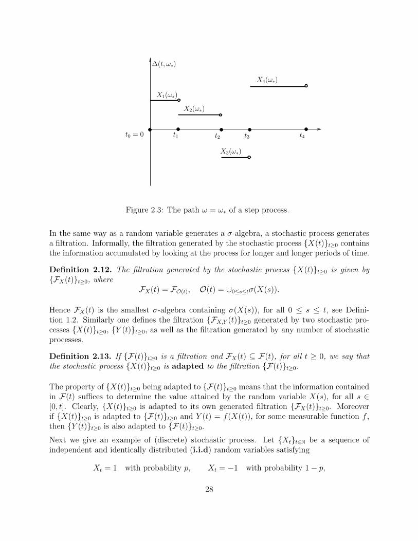
A typical path of a step process is depicted in Figure 2.3. Note that the paths of a stepprocess are right-continuous, but in general they are not left-continuous. Moreover, sinceXk(ω) = ∆(tk, ω), we can rewrite ∆(t) as

∆(t) =∞∑k

∆(tk)I[tk,tk+1).

It will be shown in Theorem 4.2 that any sufficiently regular stochastic process can beapproximated, in a suitable sense, by a sequence of step processes.

27

t0 = 0 t1 t2 t3 t4

∆(t, ω∗)

X1(ω∗)

X2(ω∗)

X3(ω∗)

X4(ω∗)

Figure 2.3: The path ω = ω∗ of a step process.

In the same way as a random variable generates a σ-algebra, a stochastic process generatesa filtration. Informally, the filtration generated by the stochastic process X(t)t≥0 containsthe information accumulated by looking at the process for longer and longer periods of time.

Definition 2.12. The filtration generated by the stochastic process X(t)t≥0 is given byFX(t)t≥0, where

FX(t) = FO(t), O(t) = ∪0≤s≤tσ(X(s)).

Hence FX(t) is the smallest σ-algebra containing σ(X(s)), for all 0 ≤ s ≤ t, see Defini-tion 1.2. Similarly one defines the filtration FX,Y (t)t≥0 generated by two stochastic pro-cesses X(t)t≥0, Y (t)t≥0, as well as the filtration generated by any number of stochasticprocesses.

Definition 2.13. If F(t)t≥0 is a filtration and FX(t) ⊆ F(t), for all t ≥ 0, we say thatthe stochastic process X(t)t≥0 is adapted to the filtration F(t)t≥0.

The property of X(t)t≥0 being adapted to F(t)t≥0 means that the information containedin F(t) suffices to determine the value attained by the random variable X(s), for all s ∈[0, t]. Clearly, X(t)t≥0 is adapted to its own generated filtration FX(t)t≥0. Moreoverif X(t)t≥0 is adapted to F(t)t≥0 and Y (t) = f(X(t)), for some measurable function f ,then Y (t)t≥0 is also adapted to F(t)t≥0.

Next we give an example of (discrete) stochastic process. Let Xtt∈N be a sequence ofindependent and identically distributed (i.i.d) random variables satisfying

Xt = 1 with probability p, Xt = −1 with probability 1− p,

28

for all t ∈ N and some p ∈ (0, 1). For a concrete realization of these random variables, wemay think of Xt as being defined on the sample space Ω∞ of the ∞-coin tosses experiment(see Appendix 1.4). In fact, letting ω = (γj)j∈N ∈ Ω∞, we may set

Xt(ω) =

−1, if γt = H,1, if γt = T .

Hence Xt : Ω→ −1, 1 is the simple random variable Xt(ω) = IAt − IAct , where At = ω ∈Ω∞ : γt = H. Clearly, FX(t) is the collection of all the events that are resolved by the firstt-tosses, which is given as indicated at the beginning of Section 1.3.

Definition 2.14. The stochastic process Mtt∈N given by

M0 = 0, Mt =t∑

k=1

Xk,

is called random walk. For p = 1/2, the random walk is said to be symmetric.

To understand the meaning of the term “random walk”, consider a particle moving on thereal line in the following way: if Xt = 1 (i.e., if the toss number t is a head), at time t theparticle moves one unit of length to the right, if Xt = −1 (i.e., if the toss number t is a head)it moves one unit of length to the left. Then Mt gives the total amount of units of lengththat the particle has travelled to the right or to the left up to time t.

Exercise 2.14. Which of the following holds?

FM(t) ⊂ FX(t), FM(t) = FX(t), FX(t) ⊂ FM(t).

Justify the answer.

The increments of the random walk are defined as follows. If (k1, . . . , kN) ∈ NN , such that1 ≤ k1 < k2 < · · · < kN , we set

∆1 = Mk1 −M0 = Mk1 , ∆2 = Mk2 −Mk1 , . . . , ∆N = MkN −MkN−1.

Hence ∆j is the total displacement of the particle from time kj−1 to time kj.

Theorem 2.4. The increments ∆1, . . . ,∆N of the random walk are independent randomvariables.

Proof. Since

∆1 = X1 + · · ·+Xk1 = g1(X1, . . . , Xk1),

∆2 = Xk1+1 + · · ·+Xk2 = g2(Xk1+1, . . . , Xk2),

.

.

∆N = XkN−1+1 + · · ·+XkN = gN(XkN−1+1, . . . , XkN ),

the result follows by Theorem 2.1.

29

The interpretation of this result is that the particle has no memory of past movements: thedistance travelled by the particle in a given interval of time is not affected by the motion ofthe particle at earlier times.

We may now define the most important of all stochastic processes.

Definition 2.15. A Brownian motion (or Wiener process) is a stochastic processW (t)t≥0 such that

(i) The paths are continuous and start from 0 almost surely, i.e., the sample points ω ∈ Ωsuch that γωW (0) = 0 and γωW is a continuous function comprise a set of probability 1;

(ii) The increments over disjoint time intervals are independent, i.e., for all 0 = t0 < t1 <· · · < tm, the random variables

W (t1)−W (t0), W (t2)−W (t1), . . . , W (tm)−W (tm−1)

are independent;

(iii) For all s < t, the increment W (t)−W (s) belongs to N (0, t− s).

Remark 2.5. Note carefully that the properties defining a Brownian motion depend onthe probability measure P. Thus a stochastic process may be a Brownian motion relativeto a probability measure P and not a Brownian motion with respect to another (possibly

equivalent) probability measure P. If we want to emphasize the probability measure Pwith respect to which a stochastic process is a Brownian motion we shall say that it is aP-Brownian motion.

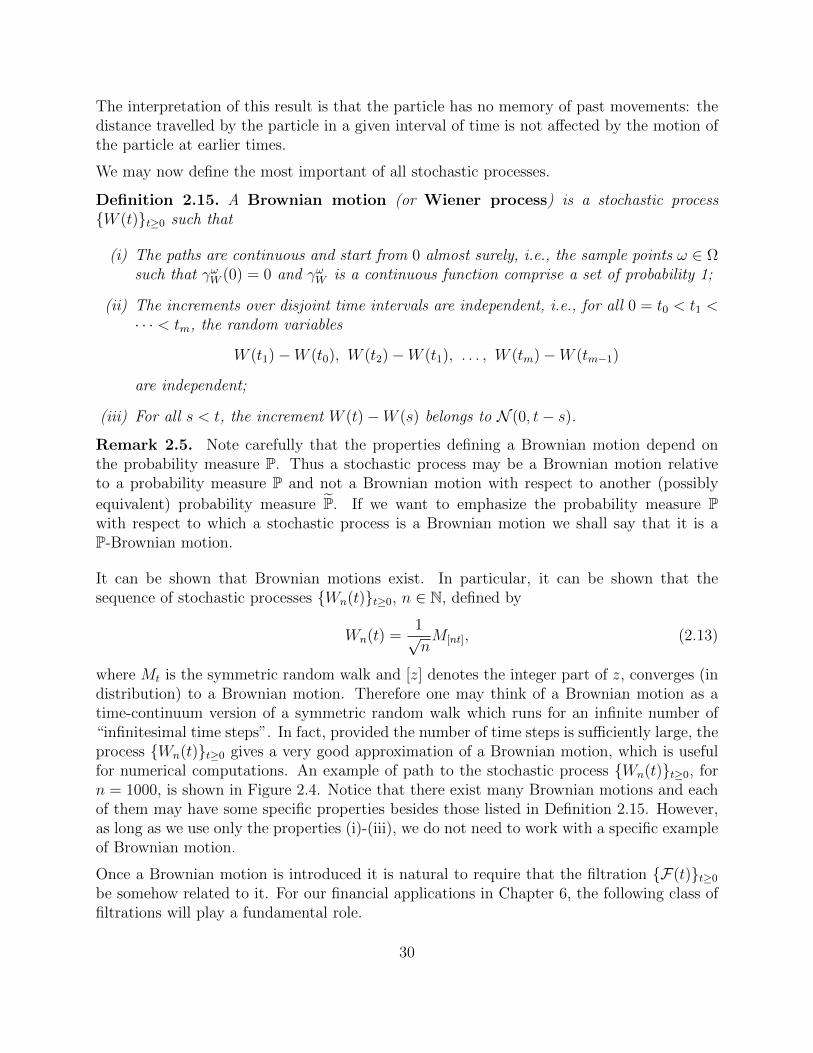
It can be shown that Brownian motions exist. In particular, it can be shown that thesequence of stochastic processes Wn(t)t≥0, n ∈ N, defined by

Wn(t) =1√nM[nt], (2.13)

where Mt is the symmetric random walk and [z] denotes the integer part of z, converges (indistribution) to a Brownian motion. Therefore one may think of a Brownian motion as atime-continuum version of a symmetric random walk which runs for an infinite number of“infinitesimal time steps”. In fact, provided the number of time steps is sufficiently large, theprocess Wn(t)t≥0 gives a very good approximation of a Brownian motion, which is usefulfor numerical computations. An example of path to the stochastic process Wn(t)t≥0, forn = 1000, is shown in Figure 2.4. Notice that there exist many Brownian motions and eachof them may have some specific properties besides those listed in Definition 2.15. However,as long as we use only the properties (i)-(iii), we do not need to work with a specific exampleof Brownian motion.

Once a Brownian motion is introduced it is natural to require that the filtration F(t)t≥0

be somehow related to it. For our financial applications in Chapter 6, the following class offiltrations will play a fundamental role.

30

200 400 600 800 1000

-10

-5

5

10

15

20

25

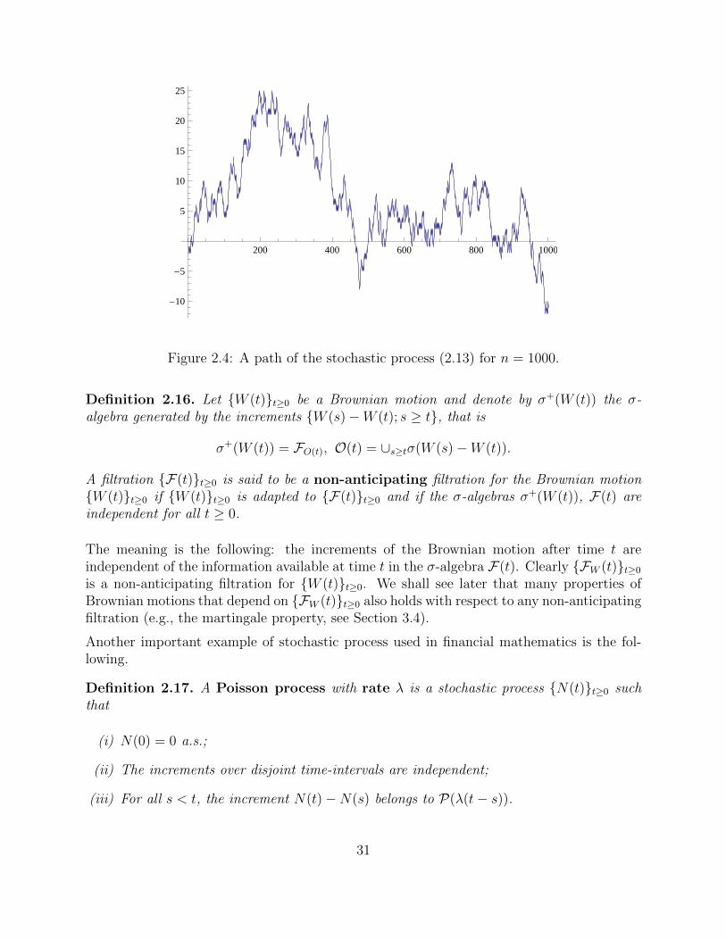
Figure 2.4: A path of the stochastic process (2.13) for n = 1000.

Definition 2.16. Let W (t)t≥0 be a Brownian motion and denote by σ+(W (t)) the σ-algebra generated by the increments W (s)−W (t); s ≥ t, that is

σ+(W (t)) = FO(t), O(t) = ∪s≥tσ(W (s)−W (t)).

A filtration F(t)t≥0 is said to be a non-anticipating filtration for the Brownian motionW (t)t≥0 if W (t)t≥0 is adapted to F(t)t≥0 and if the σ-algebras σ+(W (t)), F(t) areindependent for all t ≥ 0.

The meaning is the following: the increments of the Brownian motion after time t areindependent of the information available at time t in the σ-algebra F(t). Clearly FW (t)t≥0

is a non-anticipating filtration for W (t)t≥0. We shall see later that many properties ofBrownian motions that depend on FW (t)t≥0 also holds with respect to any non-anticipatingfiltration (e.g., the martingale property, see Section 3.4).

Another important example of stochastic process used in financial mathematics is the fol-lowing.

Definition 2.17. A Poisson process with rate λ is a stochastic process N(t)t≥0 suchthat

(i) N(0) = 0 a.s.;

(ii) The increments over disjoint time-intervals are independent;

(iii) For all s < t, the increment N(t)−N(s) belongs to P(λ(t− s)).

31

Note in particular that N(t) is a discrete random variable, for all t ≥ 0, and that, in contrastto the Brownian motion, the paths of a Poisson process are not continuous. The Poissonprocess is the building block to construct more general stochastic processes with jumps,which are popular nowadays as models for the price of certain financial assets, see [4].

2.4 Stochastic processes in financial mathematics

Remark 2.6. For more information on the financial concepts introduced in this section, seeChapter 1 in [5].

All variables in financial mathematics are represented by stochastic processes. The mostobvious example is the price of financial assets. The stochastic process representing theprice per share of a generic asset at different times will be denoted by Π(t)t≥0. Dependingon the type of asset considered, we use a different specific notation for the stochastic processmodeling its price.

Remark 2.7. We always assume that t = 0 is earlier or equal to the present time. Inparticular, the value of all financial variables is known at time t = 0. Hence, if X(t)t≥0 isa stochastic process modelling a financial variable, then X(0) is a deterministic constant.

Before presenting various examples of stochastic processes in financial mathematics, let usintroduce an important piece of terminology. An investor is said to have a short positionon an asset if the investor profits from a decrease of its price, and a long position if theinvestor profits from an increase of the price of the asset. The specific trading strategy thatleads to a short or long position on an asset depends on the type of asset considered, as weare now ready to describe in more details.

Stock price

The price per share a time t of a stock will be denoted by S(t). Typically S(t) > 0, forall t ≥ 0, however, as discussed in Section 2.2, some models allow for the possibility thatS(t) = 0 with positive probability at finite times t > 0 (risk of default). Clearly S(t)t≥0

is a stochastic process. If we have several stocks, we shall denote their price by S1(t)t≥0,S2(t)t≥0, etc. Investors who own shares of a stock are those having a long position on thestock, while investors short-selling the stock hold a short position. Concretely, an investoris short-selling N shares of a stock if the investor borrows the shares from a third partyand then sell them immediately on the market. The reason for short-selling stocks is theexpectation that the stock price will decrease in the future. If this actually happens, thenupon re-purchasing the N stock shares in the future, and returning them to the lender, theshort-seller will profit from the lower current price of the stock compared to the price at thetime of short-selling.

32

A popular model for the price of stocks is the geometric Brownian motion stochasticprocess, which is given by

S(t) = S(0) exp(αt+ σW (t)). (2.14)

Here W (t)t≥0 is a Brownian motion, α ∈ R is the instantaneous mean of log-return,σ > 0 is the instantaneous volatility, while σ2 is the instantaneous variance of thestock. Note that α and σ are constant in this model. Moreover, S(0) is the price at timet = 0 of the stock, which, according to Remark 2.7, is a deterministic constant. In Chapter 4we introduce a generalization of the geometric Brownian motion, in which the instantaneousmean of log-return and the instantaneous volatility of the stock are stochastic processesα(t)t≥0, σ(t)t≥0 (generalized geometric Brownian motion).

Exercise 2.15 (Sol. 13). Derive the density of the geometric Brownian motion (2.14) anduse the result to show that P(S(t) = 0) = 0, i.e., a stock whose price is described by ageometric Brownian motion cannot default.

Risk-free assets

A money market is a market in which the object of trading are short term loans. Moreprecisely, a money market is a type of financial market where investors can borrow and lendmoney at a given interest rate and for a period of time T ≤ 1 year5. Assets in the moneymarket (i.e., short term loans) are assumed to be risk-free, which means that their value isalways positive (that is to say, the party issuing the loan bears no risk of default). Examplesof risk-free assets in the money market are repurchase agreements (repo), certificates ofdeposit, treasure bills, etc. The stochastic process corresponding to the price per share of ageneric risk-free asset will be denoted by B(t)t∈[0,T ]. We write B(t, T ) instead of B(t) ifwe want to emphasize the dependence of the value of the loan on its maturity (this will beimportant in Section 6.6). The amount B(t) corresponds to the investor debit/credit withthe money market at time t if the amount B(0) is borrowed/lent by the investor at timet = 0. An investor lending (resp. borrowing) money has a long (resp. short) position on therisk-free asset.

The instantaneous (or continuously compounded) interest rate of a risk-free assetis the stochastic process R(t)t∈[0,T ] given by R(t) = ∂t logB(t). Hence the value of therisk-free asset at time t is

B(t) = B(0) exp

(∫ t

0

R(s) ds

), t ∈ [0, T ]. (2.15)

Although in real markets different risk-free assets have in general different (although verysimilar) interest rates6, in these notes we make the simplifying assumption that all assets in

5Loans with maturity longer than 1 year are called bonds; they will be discussed in more details inSection 6.6.

6In addition, the interest rates for borrowing and lending are usually different.

33

the money market have the same instantaneous interest rate R(t)t≥0, which we call therisk-free rate of the market. Put it differently, we assume from now on that the processR(t)t≥0 is a property of the money market, and not of the individual risk-free assets.Note that R(t) is the interest rate to borrow at time t in the “infinitesimal interval” oftime [t, t+ dt]; in the applications this corresponds typically to an “overnight loan”. Undernormal market conditions one has R(t) > 0, however negative rates are also possible. Forexample, stibor T/N (tomorrow/next), i.e., the overnight loan rate at which Swedish bankslend money to one another (interbank offered rate), has currently, 2017, a negative value.

Remark 2.8. The (average) interest rate of the money market is sometimes referred toas “the cost of money”, and the ratio B(t)/B(0) is said to express the “time-value ofmoney”. This terminology is meant to emphasize that one reason for the “time-devaluation”of money—in the sense that the purchasing power of money decreases with time—is preciselythe fact that money can grow interests by purchasing risk-free assets.

The discount process

The stochastic process D(t)t≥0 given by

D(t) = exp

(−∫ t

0

R(s) ds

)=B(0)

B(t)(2.16)

is called the discount process. If τ < t and X(t) denotes the price of an asset at time t,the quantity D(t)X(t)/D(τ), is called the t-price of the asset discounted at time τ . Whenτ = 0 we refer to D(t)X(t)/D(0) = D(t)X(t) = X∗(t) simply as the discounted priceof the asset. For instance, the discounted (at time t = 0) price of a stock with price S(t)at time t is given by S∗(t) = D(t)S(t) and has the following meaning: S∗(t) is the amountthat should be invested on the money market at time t = 0 in order that the value of thisinvestment at time t replicates the value of the stock at time t. Notice that S∗(t) < S(t)when R(t) > 0. The discounted price of the stock measures, roughly speaking, the loss inthe stock value due to the “time-devaluation” of money discussed above, see Remark 2.8.

Financial derivative

A financial derivative (or derivative security) is a contract whose value depends on theperformance of one (or more) other asset(s), which is called the underlying asset. Thereexist various types of financial derivatives, the most common being options, futures, forwardsand swaps. Financial derivatives can be traded over the counter (OTC), or in a regularizedexchange market. In the former case, the contract is stipulated between two individualinvestors, who agree upon the conditions and the price of the contract. In particular, the samederivative (on the same asset, with the same parameters) can have two different prices overthe counter. Derivatives traded in the market, on the contrary, are standardized contracts.

34

Anyone, after a proper authorization, can make offers to buy or sell derivatives in the market,in a way much similar to how stocks are traded. Let us see some examples of financialderivatives (we shall introduce more in Chapter 6).

A call option is a contract between two parties, the buyer (or owner) of the call andthe seller (or writer) of the call. The contract gives to the buyer the right, but not theobligation, to buy the underlying asset at some future time for a price agreed upon today,which is called strike price of the call. If the buyer can exercise this option only at somegiven time t = T > 0 (where t = 0 corresponds to the time at which the contract isstipulated) then the call option is called European, while if the option can be exercisedat any time in the interval (0, T ], then the option is called American. The time T > 0 iscalled maturity time, or expiration date of the call. The seller of the call is obliged tosell the asset to the buyer (at the strike price) if the latter decides to exercise the option. Ifthe option to buy in the definition of a call is replaced by the option to sell, then the optionis called a put option.

In exchange for the option, the buyer must pay a premium to the seller. Suppose that theoption is a European option with strike price K, maturity time T and premium Π0 on astock with price S(t) at time t. In which case is it then convenient for the buyer to exercisethe call? Let us define the payoff of a European call as

Y = (S(T )−K)+ := max(0, S(T )−K) (call);

similarly for a European put we set

Y = (K − S(T ))+ (put).

Note that Y is a random variable, because it depends on the random variable S(T ). Clearly, ifY > 0 it is more convenient for the buyer to exercise the option rather than buying/selling theasset on the market. Note however that the real profit for the buyer is given by N(Y −Π0),where N is the number of option contracts owned by the buyer. Typically, options are soldin stocks of 100 shares, that is to say, the minimum amount of options that one can buy is100, which cover 100 shares of the underlying asset.

One reason why investors buy calls in the market is to protect a short position on theunderlying asset. In fact, suppose that an investor short-sells 100 shares of a stock at timet = 0 with the agreement to return them to the original owner at time t0 > 0. The investorbelieves that the price of the stock will go down in the future, but of course the price maygo up instead. To avoid possible large losses, at time t = 0 the investor buys 100 shares ofan American call option on the stock expiring at T ≥ t0, and with strike price K = S(0). Ifthe price of the stock at time t0 is not lower than the price S(0) as the investor expected,then the investor will exercise the call, i.e., will buy 100 shares of the stock at the priceK = S(0). In this way the investor can return the shares to the lender with minimal losses.At the same fashion, investors buy put options to protect a long position on the underlyingasset. The reason why investors write options is mostly to get liquidity (cash) to invest in

35

other assets7.

Let us introduce some further terminology. A call (resp. put) is said to be in the money attime t if S(t) > K (resp. S(t) < K). The call (resp. put) is said to be out of the moneyif S(t) < K (resp. S(t) > K). If S(t) = K, the (call or put) option is said to be at themoney at time t. The meaning of this terminology is self-explanatory.

The premium that the buyer has to pay to the seller for the option is the price (or value)of the option. It depends on time (in particular, on the time left to expiration). Clearly,the deeper in the money is the option, the higher will be its price. Therefore the holder ofthe long position on the option is the buyer, while the seller holds the short position on theoption.

European call and put options are examples of more general contracts called Europeanderivatives. Given a function g : (0,∞) → R, a standard European derivative withpay-off Y = g(S(T )) and maturity time T > 0 is a contract that pays to its owner theamount Y at time T > 0. Here S(T ) is the price of the underlying asset (which we take tobe a stock) at time T . The function g is called pay-off function of the derivative, whileY (t) = g(S(t)) is called intrinsic value of the derivative. The term “European” refers tothe fact that the contract cannot be exercised before time T , while the term “standard”refers to the fact that the pay-off depends only on the price of the underlying at time T .The pay-off of non-standard (or exotic) European derivatives depends on the path of theasset price during the interval [0, T ]. For example, the pay-off of an Asian call is given by

Y = ( 1T

∫ T0S(t) dt−K)+.

The price at time t of a European derivative (standard or not) with pay-off Y and expirationdate T will be denoted by ΠY (t). Hence ΠY (t)t∈[0,T ] is a stochastic process. In addition,we now show that ΠY (T ) = Y holds, i.e., there exist no offers to buy or sell a derivative forless or more than Y at the time of maturity. In fact, suppose that a derivative is sold forΠY (T ) < Y “just before” it expires at time T . In this way the buyer would make the sureprofit Y −ΠY (T ) at time T , which means that the seller would loose the same amount. Onthe contrary, upon buying a derivative “just before” maturity for more than Y , the buyerwould loose Y − ΠY (T ). Thus, in a rational market, ΠY (T ) = Y (or, more precisely,ΠY (t)→ Y , as t→ T ).

A standard American derivative with pay-off function g is a contract which can beexercised at any time t ∈ (0, T ] prior or equal to its maturity and that, upon exercise, paysthe amount g(S(t)) (i.e., the intrinsic value) to the holder of the derivative. Non-standardAmerican derivatives are defined similarly as the European ones but with the further optionof earlier exercise. In these notes we are mostly concerned with European derivatives, butin Section 6.9 we also discuss briefly some properties of American call/put options.

7Of course, speculation is also an important motivation to buy/sell options. However the standard theoryof options pricing is firmly based on the interpretation of options as derivative securities and does not takespeculation into account.

36

Portfolio

The portfolio of an investor is the set of all assets in which the investor is trading. Mathe-matically it is described by a collection of N stochastic processes

h1(t)t≥0, h2(t)t≥0, . . . , hN(t)t≥0,

where hk(t) represents the number of shares of the asset k at time t in the investor portfolio.If hk(t) is positive, resp. negative, the investor has a long, resp. short, position on the assetk at time t. If Πk(t) denotes the value of the asset k at time t, then Πk(t)t≥0 is a stochasticprocess; the portfolio value is the stochastic process V (t)t≥0 given by

V (t) =N∑k=1

hk(t)Πk(t).

Remark 2.9. For modeling purposes, it is convenient to assume that an investor can tradeany fraction of shares of the assets, i.e., hk(t) : Ω→ R, rather than hk(t) : Ω→ Z.

A portfolio process is said to be self-financing in the interval [0, T ] if no cash is ever addedor withdrawn from the portfolio during the interval [0, T ]. In particular, in a self-financingportfolio, buying more shares of one asset is only possible by selling shares of another assetfor an equivalent value. The owner of a self-financing portfolio makes a profit in the timeinterval [0, T ] if V (T ) > V (0), while if V (T ) < V (0) the investor incurs in a loss. We nowintroduce the important definition of arbitrage portfolio.

Definition 2.18. A self-financing portfolio process in the interval [0, T ] is said to be anarbitrage portfolio if its value V (t)t∈[0,T ] satisfies the following properties:

(i) V (0) = 0 almost surely;

(ii) V (T ) ≥ 0 almost surely;

(iii) P(V (T ) > 0) > 0.

Hence a self-financing arbitrage portfolio is a risk-free investment in the interval [0, T ] whichrequires no initial wealth and with a positive probability to give profit. We remark that thearbitrage property depends on the probability measure P. However, it is clear that if twomeasures P and P are equivalent, then the arbitrage property is satisfied with respect to P ifand only if it is satisfied with respect to P. The guiding principle to devise theoretical modelsfor asset prices in financial mathematics is to ensure that one cannot set-up an arbitrageportfolio by investing on these assets (arbitrage-free principle).

Markets

A market in which the objects of trading are N risky assets (e.g., stocks) and M risk-freeassets in the money market is said to be “N +M dimensional”. Most of these notes focus on

37

the case of 1+1 dimensional markets in which we assume that the risky asset is a stock.A portfolio process invested in this market is a stochastic process hS(t), hB(t)t≥0, wherehS(t) is the number of shares of the stock and hB(t) the number of shares of the risk-freeasset in the portfolio at time t. The value of such portfolio is given by

V (t) = hS(t)S(t) + hB(t)B(t),

where S(t) is the price of the stock (given for instance by (2.14)), while B(t) is the value attime t of the risk-free asset, which is given by (2.15).

38

Chapter 3

Expectation

Throughout this chapter we assume that (Ω,F , F(t)t≥0,P) is a given filtered probabilityspace.

3.1 Expectation and variance of random variables

Suppose that we want to estimate the value of a random variable X before the experimenthas been performed. What is a reasonable definition for our “estimate” of X? Let us firstassume that X is a simple random variable of the form

X =N∑k=1

akIAk ,

for some finite partition Akk=1,...,N of Ω and real distinct numbers a1, . . . , aN . In this case,it is natural to define the expected value (or expectation) of X as

E[X] =N∑k=1

akP(Ak) =N∑k=1

akP(X = ak).

That is to say, E[X] is a weighted average of all the possible values attainable by X, inwhich each value is weighted by its probability of occurrence. This definition applies also forN =∞ (i.e., for discrete random variables) provided of course the infinite series converges.For instance, if X ∈ P(µ) we have

E[X] =∞∑k=0

kP(X = k) =∞∑k=0

kµke−µ

k!

= e−µ∞∑k=1

µk

(k − 1)!= e−µ

∞∑r=0

µr+1

r!= e−µµ

∞∑r=0

µr

r!= µ.

39

Exercise 3.1 (Sol. 14). Compute the expectation of binomial variables.

Now let X be a non-negative random variable and consider the sequence sXn n∈N of simplefunctions defined in Theorem 2.2. Recall that sXn converges pointwise to X as n→∞, i.e.,sXn (ω)→ X(ω), for all ω ∈ Ω (see Exercise 2.5). Since

E[sXn ] =n2n−1∑k=1

k

2nP(

k

2n≤ X <

k + 1

2n) + nP(X ≥ n), (3.1)

it is natural to introduce the following definition.

Definition 3.1. Let X : Ω → [0,∞) be a non-negative random variable. We define theexpectation of X as

E[X] = limn→∞

n2n−1∑k=1

k

2nP(

k

2n≤ X <

k + 1

2n) + nP(X ≥ n), (3.2)

i.e., E[X] = limn→∞ E[sXn ], where sX1 , sX2 , . . . is the sequence of simple functions converging

pointwise to X and defined in Theorem 2.2.

We remark that the limit in (3.2) exists, because (3.1) is an increasing sequence (see nextexercise), although this limit could be infinity. When the limit is finite we say that X hasfinite expectation. This happens for instance when X is bounded, i.e., 0 ≤ X ≤ C a.s., forsome positive constant C.

Exercise 3.2. Show that E[sXn ] is increasing in n ∈ N. Show that the limit (3.2) is finitewhen the non-negative random variable X is bounded.

Remark 3.1 (Monotone convergence theorem). It can be shown that that the limit (3.2) isthe same along any non-decreasing sequence of non-negative random variables that convergepointwise to X, hence we can use any such sequence to define the expectation of a non-negative random variable. This follows by the monotone convergence theorem, whoseprecise statement is the following: IfX1, X2, , . . . is a non-decreasing sequence of non-negativerandom variables such that Xn → X pointiwise a.s., then E[Xn]→ E[X].

Remark 3.2 (Dominated convergence theorem). The sequence of simple random variablesused to define the expectation of a non-negative random variable need not be non-decreasingeither. This follows by the dominated convergence theorem, whose precise statementis the following: if X1, X2, . . . is a sequence of non-negative random variables such thatXn → X, as n → ∞, pointiwise a.s., and supnXn ≤ Y for some non-negative randomvariable Y with finite expectation, then limn→∞ E[Xn] = E[X].

Next we extend the definition of expectation to general random variables. For this purposewe use that every random variable X : Ω→ R can be written as

X = X+ −X−,

40

whereX+ = max(0, X), X− = −min(X, 0)

are respectively the positive and negative part of X. Since X± are non-negative randomvariables, then their expectation is given as in Definition 3.1.

Definition 3.2. Let X : Ω → R be a random variable and assume that at least one of therandom variables X+, X− has finite expectation. Then we define the expectation of X as

E[X] = E[X+]− E[X−].

If X± have both finite expectation, we say that X has finite expectation or that it is anintegrable random variable. The set of all integrable random variables on Ω will be denotedby L1(Ω), or by L1(Ω,P) if we want to specify the probability measure.

Remark 3.3 (Notation). Of course the expectation of a random variable depends on the

probability measure. If another probability measure P is defined on the σ-algebra of events(not necessarily equivalent to P), we denote the expectation of X in P by E[X].

Remark 3.4 (Expectation=Lebesgue integral). The expectation of a random variable Xwith respect to the probability measure P is also called the Lebesgue integral of X over Ωin the measure P and denoted by

E[X] =

∫Ω

X(ω)dP(ω).

We shall not use this notation.

The following theorem collects some useful properties of the expectation:

Theorem 3.1. Let X, Y : Ω→ R be integrable random variables. Then the following holds:

(i) Linearity: For all α, β ∈ R, E[αX + βY ] = αE[X] + βE[Y ];

(ii) If X ≤ Y a.s. then E[X] ≤ E[Y ];

(iii) If X ≥ 0 a.s., then E[X] = 0 if and only if X = 0 a.s.;

(iv) If X, Y are independent, then E[XY ] = E[X]E[Y ].

Sketch of the proof. For all claims, the argument of the proof is divided in three steps: STEP1: Show that it suffices to prove the claim for non-negative random variables. STEP 2: Provethe claim for simple functions. STEP 3: Take the limit along the sequences sXn n∈N, sYn n∈Nof simple functions converging to X, Y . Carrying out these three steps for (i), (ii) and (iii)is simpler, so let us focus on (iv). Let X+ = f(X), X− = g(X), and similarly for Y , wheref(s) = max(0, s), g(s) = −min(0, s). By Exercise 2.4, each of (X+, Y+), (X−, Y+), (X+, Y−)and (X−, Y−) is a pair of independent (non-negative) random variables. Assume that the

41

claim is true for non-negative random variables. Then, using X = X+ −X−, Y = Y+ − Y−and the linearity of the expectation, we find

E[XY ] = E[(X+ −X−)(Y+ − Y−)]

= E[X+Y+]− E[X−Y+]− E[X+Y−] + E[X−Y−]

= E[X+]E[Y+]− E[X−]E[Y+]− E[X+]E[Y−] + E[X−]E[Y−]

= (E[X+]− E[X−])(E[Y+]− E[Y−]) = E[X]E[Y ].

Hence it suffices to prove the claim for non-negative random variables. Next assume thatX, Y are independent simple functions and write

X =N∑j=1

ajIAj , Y =M∑k=1

bkIBk .

We have

XY =N∑j=1

M∑k=1

ajbkIAjIBk =N∑j=1

M∑k=1

ajbkIAj∩Bk .

Thus by linearity of the expectation, and since the events Aj, Bk are independent, for allj, k, we have

E[XY ] =N∑j=1

M∑k=1

ajbkE[IAj∩Bk ] =N∑j=1

M∑k=1

ajbkP(Aj ∩Bk)

=N∑j=1

M∑k=1

ajbkP(Aj)P(Bk) =N∑j=1

ajP(Aj)M∑k=1

bkP(Bk) = E[X]E[Y ].

Hence the claim holds for simple functions. It follows that

E[sXn sYn ] = E[sXn ]E[sYn ].

Letting n→∞, the right hand side converges to E[X]E[Y ]. To complete the proof we haveto show that the left hand side converges to E[XY ]. This follows by applying the monotoneconvergence theorem (see Remark 3.1) to the sequence Zn = sXn s

Yn .

As |X| = X+ +X−, a random variable X is integrable if and only if E[|X|] <∞. Hence wehave

X ∈ L1(Ω)⇔ E[X] <∞⇔ E[|X|] <∞.The set of random variables X : Ω→ R such that |X|2 is integrable, i.e., E[|X|2] <∞, willbe denoted by L2(Ω) or L2(Ω,P).

Exercise 3.3 (Sol. 15). Prove the Schwarz inequality,

E[XY ] ≤√E[X2]E[Y 2], (3.3)

for all random variables X, Y ∈ L2(Ω).

42

Letting Y = 1 in (3.3), we findL1(Ω) ⊂ L2(Ω).

The covariance Cov(X, Y ) of two random variables X, Y ∈ L2(Ω) is defined as

Cov(X, Y ) = E[XY ]− E[X]E[Y ].

Two random variables are said to be uncorrelated if Cov(X, Y ) = 0. By Theorem 3.1(iv),if X, Y are independent then they are uncorrelated, but the opposite is not true in general.Consider for example the simple random variables

X =

−1 with probability 1/30 with probability 1/31 with probability 1/3

and

Y = X2 =

0 with probability 1/31 with probability 2/3

Then X and Y are clearly not independent, but

Cov(X, Y ) = E[XY ]− E[X]E[Y ] = E[X3]− 0 = 0,

since E[X3] = E[X] = 0.

Definition 3.3. The variance of a random variable X ∈ L2(Ω) is given by

Var[X] = E[(X − E[X])2].

Using the linearity of the expectation we can rewrite the definition of variance as

Var[X] = E[X2]− 2E[E[X]X] + E[X]2 = E[X2]− E[X]2 = Cov(X,X).

Note that a random variable has zero variance if and only if X = E[X] a.s., hence we mayview Var[X] as a measure of the “randomness of X”. As a way of example, let us computethe variance of X ∈ P(µ). We have

E[X2] =∞∑k=0

k2P(X = k) =∞∑k=0

k2µke−µ

k!= e−µ

∞∑k=1

k

(k − 1)!µk

= e−µ∞∑r=0

r + 1

r!µr+1 = e−µµ

∞∑r=0

µr

r!+ µ

∞∑r=0

rP(X = r) = µ+ µE[X] = µ+ µ2.

HenceVar[X] = E[X2]− E[X]2 = µ+ µ2 − µ2 = µ.

Exercise 3.4. Compute the variance of binomial random variables.

43

Exercise 3.5 (Sol. 16). Prove the following:

1. Var[αX] = α2Var[X], for all constants α ∈ R;

2. Var[X + Y ] = Var[X] + Var[Y ] + 2Cov(X, Y );

3. −√

Var[X]Var[Y ] ≤ Cov(X, Y ) ≤√

Var[X]Var[Y ]. The left (resp. right) inequalitybecomes an equality if and only if there exists a negative (resp. positive) constant a0

and a real constant b0 such that Y = a0X + b0 almost surely.

By the previous exercise, Var(X + Y ) = Var(X) + Var(Y ) holds if and only if X, Y areuncorrelated. Moreover, if we define the correlation of X, Y as

Cor(X, Y ) =Cov(X, Y )√

Var(X)Var(Y ),

then Cor(X, Y ) ∈ [−1, 1] and |Cor(X, Y )| = 1 if and only if Y is a linear function of X.The interpretation is the following: the closer is Cor(X, Y ) to 1 (resp. −1), the more thevariables X and Y have tendency to move in the same (resp. opposite) direction (for instance,(Cor(X,−2X) = −1, Cor(X, 2X) = 1). An important problem in quantitative finance is tofind correlations between the price of different assets.

Exercise 3.6. Let Mkk∈N be a random walk (not necessarily symmetric). Compute E[Mk]and Var[Mk], for all k ∈ N.

Exercise 3.7. Show that the function ‖ · ‖2 which maps a random variable Z to ‖Z‖2 =√E[Z2] is a norm in L2(Ω).

Remark 3.5 (L2-norm). The norm defined in the previous exercise is called L2 norm. Itcan be shown that it is a complete norm, i.e., if Xnn∈N ⊂ L2(Ω) is a Cauchy sequence ofrandom variables in the norm L2, then there exists a random variable X ∈ L2(Ω) such that‖Xn −X‖2 → 0 as n→∞.

Exercise 3.8 (Sol. 17). Let Wn(t)t≥0, n ∈ N, be the sequence of stochastic processesdefined in (2.13). Compute E[Wn(t)], Var[Wn(t)], Cov[Wn(t),Wn(s)]. Show that

Var(Wn(t))→ t, Cov(Wn(t),Wn(s))→ min(s, t), as n→ +∞.Exercise 3.9 (?). Let W (t)t≥0 be a Brownian motion and T > 0. Show that XT ∈N (0, 1

3T 3), where XT =

∫ T0W (t) dt.

Next we want to present a first application in finance of the theory outlined above. Inparticular we establish a sufficient condition which ensures that a portfolio is not an arbitrage.

Theorem 3.2. Let a portfolio process be given with value V (t)t≥0. Let V ∗(t) = D(t)V (t) be

the discounted portfolio value. If there exists a measure P equivalent to P such that E[V ∗(t)]is constant (independent of t), then for all T > 0 the portfolio is not an arbitrage in theinterval [0, T ].

44

Proof. Assume that the portfolio is an arbitrage in some interval [0, T ]. Then V (0) = 0almost surely; as V ∗(0) = V (0), the assumption of constant expectation in the probability

measure P givesE[V ∗(t)] = 0, for all t ≥ 0. (3.4)

Moreover P(V (T ) ≥ 0) = 1 and P(V (T ) > 0) > 0. Since P and P are equivalent, we also

have P(V (T ) ≥ 0) = 1 and P(V (T ) > 0) > 0. Since the discount process is positive, we

also have P(V ∗(T ) ≥ 0) = 1 and P(V ∗(T ) > 0) > 0. However this contradicts (3.4), due toTheorem 3.1(iii). Hence our original hypothesis that the portfolio is an arbitrage portfoliois false.

Theorem 3.2 will be applied in Chapter 6. To this purpose we shall need the followingcharacterization of equivalent probability measures.

Theorem 3.3. The following statements are equivalents:

(i) P and P are equivalent probability measures;

(ii) There exists a unique (up to null sets) random variable Z : Ω → R such that Z > 0

P-almost surely, E[Z] = 1 and P(A) = E[ZIA], for all A ∈ F .

Moreover, assuming any of these two equivalent conditions, for all random variables X suchthat XZ ∈ L1(Ω,P), we have X ∈ L1(Ω, P) and

E[X] = E[ZX]. (3.5)

Proof. The implication (i) ⇒ (ii) follows by the Radon-Nikodym theorem, whose proofcan be found for instance in [7]. As to the implication (ii) ⇒ (i), we first observe that

P(Ω) = E[ZIΩ] = E[Z] = 1. Hence, to prove that P is a probability measure, it remains toshow that it satisfies the countable additivity property: for all families Akk∈N of disjoint

events, P(∪kAk) =∑

k P(Ak). To prove this let

Bn = ∪nk=1Ak.

Clearly, ZIBn is an increasing sequence of random variables. Hence, by the monotone con-vergence theorem (see Remark 3.1) we have

limn→∞

E[ZIBn ] = E[ZIB∞ ], B∞ = ∪∞k=1Ak,

i.e.,limn→∞

P(Bn) = P(B∞). (3.6)

On the other hand, by linearity of the expectation,

P(Bn) = E[ZBn] = E[ZI∪nk=1Ak] = E[Z(IA1 + · · ·+ IAn)] =

n∑k=1

E[ZAk] =n∑k=1

P(Ak).

45

Hence (3.6) becomes∞∑k=1

P(Ak) = P(∪∞k=1Ak).

This proves that P is a probability measure. To show that P and P are equivalent, let A besuch that P(A) = 0. Since ZIA ≥ 0 almost surely, then P(A) = E[ZIA] = 0 is equivalent, byTheorem 3.1(iii), to ZIA = 0 almost surely. Since Z > 0 almost surely, then this is equivalent

to IA = 0 a.s., i.e., P(A) = 0. Thus P(A) = 0 if and only if P(A) = 0, i.e., the probability

measures P and P are equivalent. It remains to prove the identity (3.5). If X is the simplerandom variable X =

∑k akIAk , then the proof is straightforward:

E[X] =∑k

akP(Ak) =∑k

akE[ZIAk ] = E[Z∑k

akIAk ] = E[ZX].

For a general non-negative random variable X the result follows by applying (3.5) to anincreasing sequence of simple random variables converging to X and then passing to thelimit (using the monotone convergence theorem). The result for a general random variableX : Ω → R follows by applying (3.5) to the positive and negative part of X and using thelinearity of the expectation.

Remark 3.6 (Radon-Nikodym derivative). Using the Lebesgue integral notation (see Re-mark 3.4) we can write (3.5) as∫

Ω

X(ω)dP(ω) =

∫Ω

X(ω)Z(ω)dP(ω).

This leads to the formal identity dP(ω) = Z(ω)dP(ω), or Z(ω) = dP(ω)dP(ω)

, which explains why

Z is also called the Radon-Nikodym derivative of P with respect to P.

An application of Theorem 3.3 is given in Exercise 3.12 below.

Computing the expectation of a random variable

Next we discuss how to compute the expectation of a random variable X. Definition 3.1 isclearly not very useful to this purpose, unless X is a simple random variable. There existseveral methods to compute the value for E[X], some of which will be presented later in thesenotes. In this section we show that the expectation and the variance of a random variablecan be computed easily when the random variable admits a density.

Theorem 3.4. Let X : Ω→ R be a random variable and g : R→ R be a measurable functionsuch that g(X) ∈ L1(Ω). Assume that X admits the density fX . Then

E[g(X)] =

∫Rg(x)fX(x) dx.

46

In particular, the expectation and the variance of X are given by

E[X] =

∫RxfX(x) dx, Var[X] =

∫Rx2fX(x) dx−

(∫RxfX(x) dx

)2

.

Proof. We prove the theorem under the assumption that g is a simple measurable function,the proof for general functions g follows by a limit argument similar to the one used in theproof of Theorem 3.1, see Theorem 1.5.2 in [25] for the details. Hence we assume

g(x) =N∑k=1

αkIUk(x),

for some disjoint Borel sets U1, . . . , UN ⊂ R. Thus

E[g(X)] = E[∑

k

αkIUk(X)] =∑k

αkE[IUk(X)].

Let Yk = IUk(X) : Ω → R. Then Yk is the simple random variable that takes value 1 ifω ∈ Ak and 0 if ω ∈ Ack, where Ak = X ∈ Uk. Thus the expectation of Yk is given byE[Yk] = P(Ak) and so

E[g(X)] =∑k

αkP(X ∈ Uk) =∑k

αk

∫Uk

f(x) dx =

∫R

∑k

αkIUk(x)f(x) dx =

∫Rg(x)f(x) dx,

as claimed.

For instance, if X ∈ N (m,σ2), we have

E[X] =

∫Rxe−

(x−m)2

2σ2dx√2πσ2

= m,

Var[X] =

∫Rx2e−

(x−m)2

2σ2dx√2πσ2

−m2 = σ2,

which explains why we called m the expectation and σ2 the variance of the normal randomvariable X. Note in particular that, for a Brownian motion W (t)t≥0, there holds

E[W (t)−W (s)] = 0, Var[W (t)−W (s)] = |t− s|, for all s, t ≥ 0. (3.7)

Let us show that1

Cov(W (t),W (s)) = min(s, t). (3.8)

For s = t, the claim is equivalent to Var[W (t)] = t, which holds by definition of Brownianmotion (see (3.7)). For t > s we have

Cov(W (t),W (s)) = E[W (t)W (s)]− E[W (t)]E[W (s)]

= E[W (t)W (s)]

= E[(W (t)−W (s))W (s)] + E[W (s)2].

1Compare (3.8) with the result of Exercise 3.8.

47

SinceW (t)−W (s) andW (s) are independent random variables, then E[(W (t)−W (s))W (s)] =E(W (t)−W (s)]E[W (s)] = 0, and so

Cov(W (t),W (s)) = E[W (s)2] = Var[W (s)] = s = min(s, t), for t > s.

A similar argument applies for t < s.

Exercise 3.10. The moment of order n of a random variable X is the quantity µn = E[Xn],n = 1, 2, . . . . Let X ∈ N (0, σ2). Prove that

µn =

0 if n is odd

1 · 3 · 5 . . . · · · · (n− 1)σn if n is even.

Exercise 3.11 (Sol. 18). Compute the expectation and the variance of exponential randomvariables.

Exercise 3.12 (Sol. 19). Let X ∈ E(λ) an exponential random variable with intensity λ.

Given λ > 0, let

Z =λ

λe−(λ−λ)X .

Define P(A) = E[ZIA], A ∈ F . Show that P is a probability measure equivalent to P. Prove

that X ∈ E(λ) in the probability measure P.

Exercise 3.13. Compute the expectation and the variance of Cauchy distributed randomvariables. Compute the expectation and the variance of Levy distributed random variables.

Exercise 3.14. Compute the expectation and the variance of the geometric Brownian mo-tion (2.14).

Exercise 3.15. Show that the paths of the Brownian motion have unbounded linear variation.Namely, given 0 = t0 < t1 < · · · < tn = t with tk − tk−1 = h, for all k = 1, . . . , n, show that

E[n∑k=1

|W (tk)−W (tk−1)|]→∞, as n→∞.

(However, Brownian motions have finite quadratic variation, see Section 3.2).

A result similar to Theorem 3.4 can be used to compute the correlation between two randomvariables that admit a joint density.

Theorem 3.5. Let X, Y : Ω → R be two random variables with joint density fX,Y : R2 →[0,∞) and let g : R2 → R be a measurable function such that g(X, Y ) ∈ L1(Ω). Then

E[g(X, Y )] =

∫R2

g(x, y)fX,Y (x, y) dx dy.

In particular, for X, Y ∈ L2(Ω),

Cov(X, Y ) =

∫R2

xyfX,Y (x, y) dx dy −∫RxfX(x) dx

∫RyfY (y) dy,

48

where

fX(x) =

∫RfX,Y (x, y) dy, fY (y) =

∫RfX,Y (x, y) dx

are the (marginal) densities of X and Y .

Exercise 3.16. Show that if X1, X2 : Ω→ R are jointly normally distributed with covariantmatrix C = (Cij)i,j=1,2, then Cij = Cov(Xi, Xj).

Combining the results of Exercises 2.11 and 3.16, we see that the parameter ρ in Equa-tion (2.10) is precisely the correlation of the two jointly normally distributed random vari-ables X, Y . It follows by Remark 2.3 that two jointly normally distributed random variablesare independent if and only if they are uncorrelated. Recall that for general random variables,independence implies uncorrelation, but the opposite is in general not true.

Characteristic function

In this section, and occasionally in the rest of the notes, we shall need to take the expectationof a complex-valued random variable Z : Ω → C. Letting Z = Re(Z) + iIm(Z), theexpectation of Z is the complex number defined by

E[Z] = E[Re(Z)] + iE[Im(Z)].

Definition 3.4. Let X ∈ L1(Ω). The function θX : R→ C given by

θX(u) = E[eiuX ]

is called the characteristic function of X. The positive, real-valued function MX(u) =E[euX ], when it exists in some neighborhood of u = 0, is called the moment-generatingfunction of X.

Note that if the random variable X admits the density fX , then

θX(u) =

∫ReiuxfX(x) dx,

i.e., the characteristic function is the inverse Fourier transform of the density. Table 3.1contains some examples of characteristic functions.

Remark 3.7. While θX is defined for all u ∈ R, the moment-generating function of arandom variable may be defined only in a subset of the real line, or not defined at all (seeExercise 3.17). For instance, when X ∈ E(λ) we have

MX(u) = E[euX ] = λ

∫ ∞0

e(u−λ)x dx =

+∞ if u ≥ λ(1− u/λ)−1 if u < λ

Hence MX(u) is defined (as a positive function) only for u < λ.

Exercise 3.17. Show that Cauchy random variables do not have a well-defined moment-generating function.

49

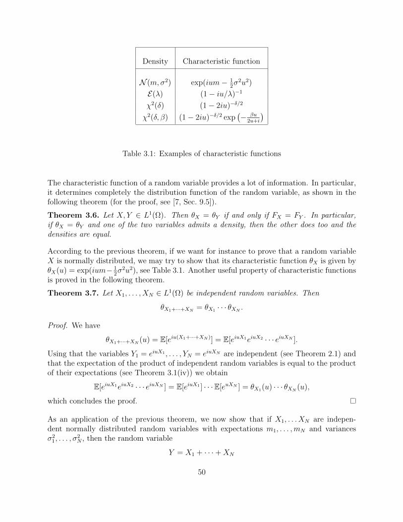
Density Characteristic function

N (m,σ2) exp(ium− 12σ2u2)

E(λ) (1− iu/λ)−1

χ2(δ) (1− 2iu)−δ/2

χ2(δ, β) (1− 2iu)−δ/2 exp(− βu

2u+i

)

Table 3.1: Examples of characteristic functions

The characteristic function of a random variable provides a lot of information. In particular,it determines completely the distribution function of the random variable, as shown in thefollowing theorem (for the proof, see [7, Sec. 9.5]).

Theorem 3.6. Let X, Y ∈ L1(Ω). Then θX = θY if and only if FX = FY . In particular,if θX = θY and one of the two variables admits a density, then the other does too and thedensities are equal.

According to the previous theorem, if we want for instance to prove that a random variableX is normally distributed, we may try to show that its characteristic function θX is given byθX(u) = exp(ium− 1

2σ2u2), see Table 3.1. Another useful property of characteristic functions

is proved in the following theorem.

Theorem 3.7. Let X1, . . . , XN ∈ L1(Ω) be independent random variables. Then

θX1+···+XN = θX1 · · · θXN .

Proof. We have

θX1+···+XN (u) = E[eiu(X1+···+XN )] = E[eiuX1eiuX2 · · · eiuXN ].

Using that the variables Y1 = eiuX1 , . . . , YN = eiuXN are independent (see Theorem 2.1) andthat the expectation of the product of independent random variables is equal to the productof their expectations (see Theorem 3.1(iv)) we obtain

E[eiuX1eiuX2 · · · eiuXN ] = E[eiuX1 ] · · ·E[euXN ] = θX1(u) · · · θXN (u),

which concludes the proof.

As an application of the previous theorem, we now show that if X1, . . . XN are indepen-dent normally distributed random variables with expectations m1, . . . ,mN and variancesσ2

1, . . . , σ2N , then the random variable

Y = X1 + · · ·+XN

50

is normally distributed with mean m and variance σ2 given by

m = m1 + · · ·+mN , σ2 = σ21 + · · ·+ σ2

N . (3.9)

In fact,

θX1+···+XN (u) = θX1(u) · · · θXN (u) = eium1− 12σ2

1u2 · · · eiumN− 1

2σ2Nu

2

= eium−12σ2u2

.

The right hand side of the previous equation is the characteristic function of a normalvariable with expectation m and variance σ2 given by (3.9). Thus Theorem 3.6 implies thatX1 + · · ·+XN ∈ N (m,σ2).

Exercise 3.18 (?). Let X1 ∈ N (m1, σ21), . . . , XN ∈ N (mN , σ

2N), N ≥ 2, be independent.

Show that Y =∑N

k=1(Xk/σk)2 ∈ χ2(N, β) where β = (m1/σ1)2 + · · · + (mN/σN)2 (compare

with Exercise 2.8).

Exercise 3.19. Let X, Y ∈ N (0, 1) be independent and jointly normally distributed. Showthat the random variable Z defined by

Z =

Y/X for X 6= 0,

0 otherwise

is Cauchy distributed.

In a similar fashion, we define the characteristic function of the vector-valued random variableX = (X1, . . . , Xn) as θX : Rn → C,

θX(u1, . . . , un) = E[eu1X1+u2X2+···+unXn ].

For instance, it can be shown that two random variables X1, X2 are jointly normal withmean m = (m1 m2) and covariance matrix C = (Cij)i,j=1,2 if and only if the characteristicfunction of X = (X1, X2) is given by

θX(u1, u2) = eimu−12uTC u, u =

(u1

u2

).

Exercise 3.20 (?). Let X1, X2 ∈ N (0, 1) be independent and define

Y1 = aX1 + bX2, Y2 = cX1 + dX2,

for some constants a, b, c, d ∈ R. Assume that the matrix

A =

(a bc d

)is invertible. Show that Y1, Y2 are jointly normally distributed with zero mean and covariantmatrix C = AAT .

51

Exercise 3.21. Let W (t)t≥0 be a Brownian motion and t1 < t2. Show that W (t1), W (t2)are jointly normally distributed with zero mean and covariance matrix

C =

(t1 t1t1 t2

).

Exercise 3.22. Let X, Y ∈ L1(Ω) be independent random variables with densities fX , fY .Show that X + Y has the density

fX+Y (x) =

∫RfX(x− y)fY (y) dy.

Remark: The right hand side of the previous identity defines the convolution product ofthe functions fX , fY .

The characteristic function is also very useful to establish whether two random variables areindependent, as shown in the following exercise.

Exercise 3.23. Let X, Y ∈ L1(Ω) and define their joint characteristic function as

θX,Y (u, v) = E[eiuX+ivY ], u, v ∈ R.

Show that X, Y are independent if and only if θX,Y (u, v) = θX(u)θY (v).

3.2 Quadratic variation of stochastic processes

We continue this chapter by discussing the important concept of quadratic variation. Weintroduce this concept to measure how “wild” a stochastic process oscillates in time, whichin financial mathematics is a measure of the volatility of an asset price.

Let X(t)t≥0 be a stochastic process. A partition of the interval [0, T ] is a set of pointsΠ = t0, t1, . . . tm such that

0 = t0 < t1 < t2 < · · · < tm = T.

The size of the partition is given by

‖Π‖ = maxj=0,...,m−1

(tj+1 − tj).

To measure the amount of oscillations of X(t)t≥0 in the interval [0, T ] along the partitionΠ, we compute

QΠ(ω) =m−1∑j=0

(X(tj+1, ω)−X(tj, ω))2.

52

Note carefully that QΠ is a random variable and that it depends on the partition. Forexample, let ∆(s)s≥0 be the step process

∆(s, ω) =∞∑k=0

Xk(ω)I[sk,sk+1).

Then if the partition Π = 0, t1, . . . , tm = T is such that sk−1 < tk < sk, for all k =1, 2, . . .m, we have

QΠ(ω) = (X2(ω)−X1(ω))2 + (X3(ω)−X2(ω))2 + · · ·+ (Xm+1(ω)−Xm(ω))2.

However if two points in the partition belong to the same interval [sk, sk+1), the variationwithin these two instants of time clearly gives no contribution to the total variation QΠ.

To define the quadratic variation of the stochastic process X(t)t≥0, we compute QΠn alonga sequence Πnn∈N of partitions to the interval [0, T ] such that ‖Πn‖ → 0 as n → ∞ andthen we take the limit of QΠn as n→∞. Since QΠnn∈N is a sequence of random variables,there are several ways to define its limit as n → ∞. The precise definition that we adoptis that of L2-quadratic variation, in which the limit is taken in the norm ‖ · ‖2 defined inExercise 3.5.

Definition 3.5. We say that the stochastic process X(t)t≥0 has L2-quadratic variation[X,X](T ) in the interval [0, T ] along the sequence of partitions Πnn∈N if

limn→∞

E

m(n)−1∑j=0

(X(t(n)j+1)−X(t

(n)j ))2 − [X,X](T )

2 = 0,

where m(n) + 1 is the number of points in the partition Πn = t0, t(n)1 , t

(n)2 , . . . , t

(n)m(n)−1, T.

Remark 3.8. If the limit in the previous definition does not exist, the quadratic variationcannot be defined as we did (an alternative definition is possible, but we shall not need it).

Note that the quadratic variation is a random variable that depends in general on thesequence of partitions of the interval [0, T ] along which it is computed, although this is notreflected in our notation [X,X](T ). However for several important examples of stochasticprocesses—and in particular for all applications considered in these notes—the quadraticvariation is independent of the sequence of partitions. To distinguish this important specialcase, we shall use the following (standard) notation:

dX(t)dX(t) = σ(t)dt,

to indicate that the quadratic variation of the stochastic process X(t)t≥0 in any interval[0, T ] is given by

[X,X](T ) =

∫ T

0

σ(t) dt

53

independently from the sequence of partitions of the interval [0, T ] along which it is computed.Here σ(t)t≥0 is a stochastic process called rate of quadratic variation of X(t)t≥0 andwhich measures how fast quadratic variation accumulates in time.

Now we show that if the paths of the stochastic process X(t)t≥0 are sufficiently regular,then its quadratic variation is zero along any sequence of partitions.

Theorem 3.8. Assume that the paths of the stochastic process X(t)t≥0 satisfy

P(|X(t)−X(s)| ≤ C|t− s|γ) = 1, (3.10)

for all t, s ≥ 0 and for some positive constants C > 0, γ > 1/2. Then

dX(t)dX(t) = 0.

Proof. We have

E

m(n)−1∑j=0

(X(t(n)j+1)−X(t

(n)j ))2

2 ≤ C4E

m(n)−1∑j=0

(t(n)j+1 − t(n)

j )2γ

2= C4E

m(n)−1∑j=0

(t(n)j+1 − t(n)

j )2γ−1(t(n)j+1 − t(n)

j )

2 .Now we use that t

(n)j+1 − t(n)

j ≤ ‖Πn‖ and∑

j(t(n)j+1 − t(n)

j ) = T , so that

E

m(n)−1∑j=0

(X(t(n)j+1)−X(t

(n)j ))2

2 ≤ (C2‖Πn‖2γ−1T)2 → 0, as ‖Πn‖ → 0.

As a special important case we have that

dtdt = 0. (3.11)

Next we compute the quadratic variation of Brownian motions.

Theorem 3.9. For a Brownian motion W (t)t≥0 there holds

dW (t)dW (t) = dt. (3.12)

Proof. Let

QΠn(ω) =

m(n)−1∑j=0

(W (t(n)j+1, ω)−W (t

(n)j , ω))2,

54

where we recall that m(n) + 1 is the number of points in the partition Πn of [0, T ]. Wecompute

E[(QΠn − T )2] = E[Q2Πn ] + T 2 − 2TE[QΠn ].

But

E[QΠn ] =

m(n)−1∑j=0

E[(W (t(n)j+1)−W (t

(n)j ))2] =

m(n)−1∑j=0

Var[W (t(n)j+1)−W (t

(n)j )]

=

m(n)−1∑j=0

(t(n)j+1 − t(n)

j ) = T.

Hence we have to prove thatlim‖Πn‖→0

E[Q2Πn ]− T 2 = 0,

or equivalently (as we have just proved that E[QΠn ] = T ),

lim‖Πn‖→0

Var(QΠn) = 0. (3.13)

Since the increments of a Brownian motion are independent, we have

Var(QΠn) =

m(n)−1∑j=0

Var[(W (t(n)j+1)−W (t

(n)j ))2] =

m(n)−1∑j=0

E[(W (t(n)j+1)−W (t

(n)j ))4]

−m(n)−1∑j=0

E[(W (t(n)j+1)−W (t

(n)j ))2]2

Now we use that

E[(W (t(n)j+1)−W (t

(n)j ))2] = Var[W (t

(n)j+1)−W (t

(n)j )] = t

(n)j+1 − t(n)

j ,

and, as it follows by Exercise 3.10,

E[(W (t(n)j+1)−W (t

(n)j ))4] = 3(t

(n)j+1 − t(n)

j )2.

We conclude that

Var[QΠn ] = 2

m(n)−1∑j=0

(t(n)j+1 − t(n)

j )2 ≤ 2‖Πn‖T → 0, as ‖Πn‖ → 0,

which proves (3.13) and thus the theorem.

Remark 3.9 (No-where differentiability of Brownian motions). Combining Theorem 3.9 andTheorem 3.8, we conclude that the paths of a Brownian motion W (t)t≥0 cannot satisfythe regularity condition (3.10). In fact, while the paths of a Brownian motion are a.s.continuous by definition, they turn out to be no-where differentiable, in the sense thatthe event ω ∈ Ω : γωW ∈ C1 is a null set. A proof of this can be found for instance in [9].

55

Finally we need to consider a slight generalization of the concept of quadratic variation.

Definition 3.6. We say that two stochastic processes X1(t)t≥0 and X2(t)t≥0 have L2-cross variation [X1, X2](T ) ∈ R in the interval [0, T ] along the sequence of partitionsΠnn∈N, if

limn→∞

E

m(n)−1∑j=0

(X1(t(n)j+1)−X1(t

(n)j ))(X2(t

(n)j+1)−X2(t

(n)j ))− [X1, X2](T )

2 = 0,

where m(n) + 1 is the number of points in the partition Πn.

As for the quadratic variation of a stochastic process, we use a special notation to express thatthe cross variation of two stochastic processes is independent of the sequence of partitionsalong which it is computed. Namely, we write

dX1(t)dX2(t) = ξ(t) dt,

to indicate that the cross variation [X1, X2](T ) equals∫ T

0ξ(t) dt along any sequence of par-

titions Πnn∈N of the interval [0, T ]. The following generalization of Theorem 3.8 is easilyestablished.

Theorem 3.10. Assume that the paths of the stochastic processes X1(t)t≥0, X2(t)t≥0

satisfy

P(|X1(t)−X1(s)| ≤ C|t− s|γ) = 1, P(|X2(t)−X2(s)| ≤ C|t− s|λ) = 1,

for all s, t ≥ 0 and some positive constants C, γ, λ such that γ+λ > 1/2. Then dX1(t)dX2(t) =0.

Exercise 3.24. Prove the theorem.

As a special case we find thatdW (t)dt = 0. (3.14)

It is important to memorize the identities (3.11), (3.12) and (3.14), as they will be usedseveral times in the following chapters.

Exercise 3.25 (?). Let W1(t)t≥0, W2(t)t≥0 be two independent Brownian motions. Showthat dW1(t)dW2(t) = 0.

3.3 Conditional expectation

Recall that the expectation value E[X] is an estimate on the average value of the randomvariable X. This estimate does not depend on the σ-algebra F , nor on any sub-σ-algebra

56

thereof. However, if some information is known in the form of a σ-algebra G, then oneexpects to be able to improve the estimate on the value of X. To quantify this we introducethe definition of “expected value of X given G”, or conditional expectation, which we denoteby E[X|G]. We want the conditional expectation to verify the following properties:

(i) If X is G-measurable, then it should hold that E[X|G] = X, because the informationprovided by G is sufficient to determine X;

(ii) If X is independent of G, then E[X|G] = E[X], because the occurrence of the eventsin G does not effect the probability distribution of X;

Note that (i) already indicates that E[X|G] is a random variable. To begin with we definethe conditional expectation of a random variable X with respect to an event A ∈ F . Let’sassume first that X is the simple random variable

X =N∑k=1

akIAk .

Let B ∈ F : P(B) > 0 and P(Ak|B) = P(Ak∩B)P(B)

be the conditional probability of Ak given B,see Definition 1.6. It is natural to define the conditional expectation of X given the event Bas

E[X|B] =N∑k=1

akP(Ak|B).

Moreover, since

XIB =N∑k=1

akIAkIB =N∑k=1

akIAk∩B,

we also have the identity E[X|B] = E[XIB ]P(B)

. We use the latter identity to define the conditionalexpectation given B of general random variables.

Definition 3.7. Let X ∈ L1(Ω) and B ∈ F . When P(B) > 0 we define the conditionalexpectation of X given the event B as

E[X|B] =E[XIB]

P(B).

When P(B) = 0 we define E[X|B] = E[X].

Remark 3.10. Using the Lebesgue integral notation of the expectation, see Remark 3.4,we may rewrite

E[X|B] =1

P(B)

∫B

X(ω)dP(ω),

which shows that the conditional expectation of a random variable X with respect to anevent B is just the average of X within B.

57

Note that E[X|B] is a deterministic constant. Next we discuss the concept of conditionalexpectation given a σ-algebra G. We first assume that G is generated by a (say, finite)partition Akk=1,...,M of Ω, see Exercise 1.4. Then it is natural to define

E[X|G] =M∑k=1

E[X|Ak]IAk . (3.15)

Note that E[X|G] is a G-measurable simple function. It will now be shown that (3.15)satisfies the identity

E[E[X|G]|B] = E[X|B], for all B ∈ G : P(B) > 0. (3.16)

In fact,

P(B)E[E[X|G]|B] = E[E[X|G]IB]

= E[M∑k=1

E[X|Ak]IAkIB]

=M∑k=1

E[E[X|Ak]IAk∩B]

=M∑k=1

E[E[XIAk ]P(Ak)

IAk∩B]

=M∑k=1

1

P(Ak)E[XIAk ]E[IAk∩B].

Since A1, . . . , AM is a partition of Ω, there exists I ⊂ 1, . . . ,M such that B = ∪k∈IAk;hence the above sum may be restricted to k ∈ I. Since E[IAk∩B] = E[IAk ] = P(Ak), for k ∈ I,we obtain

P(B)E[E[X|G]|B] =∑k∈I

E[XIAk ] = E[XI∪k∈IAk ] = E[XIB],

by which (3.16) follows.

Exercise 3.26. What is the interpretation of (3.16)?

The conditional expectation of a random variable with respect to a general σ-algebra canbe constructed explicitly only in some special cases (see for instance Theorem 3.14 below).However an abstract definition is still possible, which we give after the following theorem.

Theorem 3.11. Let G be a sub-σ-algebra of F and X ∈ L1(Ω). If Y1, Y2 ∈ L1(Ω) areG-measurable and satisfy

E[Yi|A] = E[X|A], for i = 1, 2 and all A ∈ G : P(A) > 0, (3.17)

then Y1 = Y2 a.s.

58

Proof. We want to prove that P(B) = 0, where

B = ω ∈ Ω : Y1(ω) 6= Y2(ω).

Let B+ = Y1 > Y2 and assume P(B+) > 0. Then, by (3.17) and Definition 3.7,

E[(Y1 − Y2)IB+ ] = E[Y1IB+ ]− E[Y2IB+ ] = P(B+)(E[Y1|B+]− E[Y2|B+]) = 0.

By Theorem 3.1(iii), this is possible if and only if (Y1 − Y2)IB+ = 0 a.s., which entailsP(B+) = 0. At the same fashion one proves that P(B−) = 0, where P(B−) = Y1 < Y2.Hence P(B) = P(B+) + P(B−) = 0, as claimed.

Theorem 3.12 (and Definition). Let X ∈ L1(Ω) and G be a sub-σ-algebra of F . Thereexists a G-measurable random variable E[X|G] ∈ L1(Ω) such that

E[E[X|G]|A] = E[X|A], for all A ∈ G : P(A) > 0. (3.18)

The random variable E[X|G], which by Theorem 3.11 is uniquely defined up to a null set, iscalled the conditional expectation of X given the σ-algebra G. If G is the σ-algebragenerated by a random variable Y , i.e., G = σ(Y ), we write E[X|G] = E[X|Y ].

Proof. See [25, Appendix B].

Remark 3.11. Following Remark 3.3, we denote by E[X|G] the conditional expectation of

X in a new probability measure P, not necessarily equivalent to P.

We continue this section with a list of properties satisfied by the conditional expectation.

Theorem 3.13. Let X, Y ∈ L1(Ω). The following properties hold almost surely:

(i) E[E[X|G]] = E[X];

(ii) If X is G-measurable, then E[X|G] = X;

(iii) If H ⊂ G is a sub-σ-algebra, then E[E[X|G]|H] = E[X|H];

(iv) Linearity: E[αX + βY |G] = αE[X|G] + βE[Y |G], for all α, β ∈ R;

(v) If G consists of trivial events only, then E[X|G] = E[X];

(vi) If X is independent of G, then E[X|G] = E[X];

(vii) If X is G-measurable, then E[XY |G] = XE[Y |G];

(viii) If X ≤ Y then E[X|G] ≤ E[Y |G].

59

Proof. (i) Replace A = Ω into (3.18).

(ii) Note that (3.17) is satisfied by Y1 = E[X|G] and Y2 = X; hence when X is G-measurable,we have E[X|G] = X a.s., by uniqueness.

(iii) Using (3.18), and since H ⊂ G, the random variables E[E[X|G]|H], E[X|G] and E[X|H]satisfy

E[E[E[X|G]|H]|A] = E[E[X|G]|A],

E[E[X|G]|A] = E[X|A],

E[E[X|H]|A] = E[X|A],

for all A ∈ H : P(A) > 0. It follows that

E[E[E[X|G]|H]|A] = E[E[X|H]|A]

and thus by uniqueness the claim follows.

(iv) Linearity follows easily by (3.18).

(v) This again follows at once by (3.18).

(vi) E[X|G] is uniquely characterized by the identity (3.18). As X is independent of G, therandom variables X and IA are independent, for all A ∈ G, hence E[X|A] = E[XIA]/P(A) =E[X]E[IA]/P(A) = E[X] = E[E[X]|A]. Hence (3.18) becomes E[E[X|G]|A] = E[E[X]|A], forall A ∈ G with positive probability, which implies the claim.

(vii) The proof of this property is more complicated and we refer to [7] for a complete proof.For a simple taste of the argument, consider the case when G is generated by a partitionAkk∈N of Ω and consider the G-measurable simple random variable X =

∑akIAk . Then

in this case we have obviously E[XY |Ak] = XE[Y |Ak], for all k ∈ N, since X is constant inAk. Replacing in (3.15) proves the claim for this special case.

(viii) This follows again by (3.18) and the fact that

X, Y G −measurable and X ≤ Y ⇒ E[X|A] ≤ E[Y |A], for all A ∈ G with P(A) > 0.

The details are left as an (easy) exercise.

Exercise 3.27. Give the missing details in the proofs of (iv), (v), (viii) in Theorem 3.13.

Exercise 3.28 (Sol. 20). The purpose of this exercise is to show that the conditional expec-tation is the best estimator of a random variable when some information is given in the formof a sub-σ-algebra. Let X ∈ L1(Ω) and G ⊆ F be a sub-σ-algebra. Define Err = X−E[X|G].Show that E[Err] = 0 and

Var[Err] = minY

Var[Y −X],

where the minimum is taken with respect to all G-measurable random variables Y .

60

An explicit closed formula for the conditional expectation of a random variable can rarely befound. One important exception is presented in the following theorem, which will be usedmultiple times in the sequel.

Theorem 3.14. Let X, Y : Ω → R be two random variables and G a sub-σ-algebra of Fsuch that X is G-measurable and Y is independent of G. Then for any measurable functiong : R2 → [0,∞), the function f : R→ [0,∞) defined by

f(x) = E[g(x, Y )]

is measurable and moreoverE[g(X, Y )|G] = f(X).

Proof of a special case. (See [7] for a complete proof). Assume that G is generated by apartition Akk∈N and that X is the G-measurable simple random variable X =

∑k akIAk .

ThenE[f(X)IAk ] = E[f(

∑ajIAj)IAk ] = f(ak)E[IAk ] = f(ak)P(Ak).

Moreover, since Y is independent of IAk , for all k ∈ N, then

E[g(X, Y )IAk ] = E[g(ak, Y )IAk ] = E[g(ak, Y )]E[IAk ] = f(ak)P(Ak).

The proof of this special case of the theorem now follows by (3.15).

Remark 3.12. The meaning of Theorem 3.14 is that, under the stated assumptions, wecan compute the random variable E[g(X, Y )|G] as if X were a deterministic constant.

3.4 Martingales

A martingale is a stochastic process which has no tendency to rise or fall. The precisedefinition is the following:

Definition 3.8. A stochastic process M(t)t≥0 is called a martingale relative to the fil-tration F(t)t≥0 if it is adapted to F(t)t≥0, M(t) ∈ L1(Ω) for all t ≥ 0, and

E[M(t)|F(s)] = M(s), for all 0 ≤ s ≤ t, (3.19)

for all t ≥ 0.

Hence a stochastic process is martingale if the information available up to time s does nothelp to predict whether the stochastic process will raise or fall after time s.

Remark 3.13. If the condition (3.19) is replaced by E[M(t)|F(s)] ≥ M(s), for all 0 ≤s ≤ t, the stochastic process M(t)t≥0 is called a sub-martingale. The interpretationis that M(t) has no tendency to fall, but our expectation is that it will increase. If thecondition (3.19) is replaced by E[M(t)|F(s)] ≤ M(s), for all 0 ≤ s ≤ t, the stochasticprocess M(t)t≥0 is called a super-martingale. The interpretation is that M(t) has nottendency to rise, but our expectation is that it will decrease.

61

Remark 3.14. If we want to emphasize that the martingale property is satisfied with respectto the probability measure P, we shall say that M(t)t≥0 is a P-martingale.

Since the conditional expectation of a random variable X is uniquely determined by (3.18),then the property (3.19) is satisfied if and only if

E[M(s)IA] = E[M(t)IA], for all 0 ≤ s ≤ t and for all A ∈ F(s). (3.20)

In particular, letting A = Ω, we obtain that the expectation of a martingale is constant, i.e.,

E[M(t)] = E[M(0)], for all t ≥ 0. (3.21)

Combining the latter result with Theorem 3.2, we obtain the following sufficient conditionfor no arbitrage.

Theorem 3.15. Let a portfolio be given with value V (t)t≥0. If there exists a measure

P equivalent to P and a filtration F(t)t≥0 such that the discounted value of the portfolioV ∗(t)t≥0 is a martingale, then the portfolio is not an arbitrage.

Proof. The assumption is that

E[D(t)V (t)|F(s)] = D(s)V (s), for all 0 ≤ s ≤ t.

Hence, by (3.21), E[D(t)V (t)] = E[D(0)V (0)] = E[V (0)]. The result follows by Theorem 3.2.

Theorem 3.16. Let F(t)t≥0 be a non-anticipating filtration for the Brownian motionW (t)t≥0. Then W (t)t≥0 is a martingale relative to F(t)t≥0.

Proof. The martingale property for s = t, i.e., E[W (t)|F(t)] = W (t), follows by the factW (t) is F(t)-measurable, and thus Theorem 3.13(ii) applies. For 0 ≤ s < t we have

E[W (t)|F(s)] = E[(W (t)−W (s))|F(s)] + E[W (s)|F(s)],

= E[W (t)−W (s)] +W (s) = W (s),

where we used that W (t)−W (s) is independent of F(s), and so E[(W (t)−W (s))|F(s)] =E[(W (t)−W (s))] by Theorem 3.13(vi), and the fact that W (s) is F(s)-measurable (and soE[W (s)|F(s)] = W (s)).

Exercise 3.29 (?). Consider the stochastic process Z(t)t≥0 given by

Z(t) = exp(σW (t)− 1

2σ2t),

where W (t)t≥0 is a Brownian motion and σ ∈ R is a constant. Let F(t)t≥0 be anon-anticipating filtration for W (t)t≥0. Show that Z(t)t≥0 is a martingale relative toF(t)t≥0.

62

Brownian motions are martingales, have a.s. continuous paths and have quadratic variationt in the interval [0, t], see Theorem 3.9. The following theorem shows that these threeproperties characterize Brownian motions and is often used to prove that a given stochasticprocess is a Brownian motion. The proof can be found in [17].

Theorem 3.17 (Levy characterization theorem). Let M(t)t≥0 be a martingale relativeto a filtration F(t)t≥0. Assume that (i) M(0) = 0 a.s., (ii) the paths t→M(t, ω) are a.s.continuous and (iii) dM(t)dM(t) = dt. Then M(t)t≥0 is a Brownian motion and F(t)t≥0

a non-anticipating filtration thereof.

Exercise 3.30 (Sol. 21). Let N(t)t≥0 be a Poisson process generating the filtration FN(t)t≥0.Show that (i) N(t)t≥0 is a sub-martingale relative to FN(t)t≥0 and (ii) the so-called com-pound Poisson process N(t)− λtt≥0 is a martingale relative toFN(t)t≥0, where λ isthe rate of the Poisson process (see Definition 2.17).

Exercise 3.31 (?). Let F(t)t∈[0,T ] be a filtration and M(t)t∈[0,T ] be a stochastic processadapted to F(t)t∈[0,T ] such that M(t) ∈ L1(Ω), for all t ∈ [0, T ]. Show that M(t)t∈[0,T ] isa martingale if and only if there exists a F(T )-measurable random variable H ∈ L1(Ω) suchthat

M(t) = E[H|F(t)].

Now assume that Z(t)t≥0 is a martingale such that Z(t) > 0 a.s. and E[Z(t)] = 1, for all

t ≥ 0. By Theorem 3.3, the map P : F → [0, 1] given by

P(A) = E[Z(T )IA], A ∈ F (3.22)

is a probability measure equivalent to P, for all T > 0. Note that P depends on T > 0 andP = P, for T = 0. The dependence on T is however not reflected in our notation. As usual,the (conditional) expectation in the probability measure P will be denoted E. The relation

between E and E is revealed in the following theorem.

Theorem 3.18. Let Z(t)t≥0 be a martingale such that Z(t) > 0 a.s. and E[Z(t)] = 1, for

all t ≥ 0. Let T > 0 and let P be the probability measure equivalent to P defined by (3.22).Let t ∈ [0, T ] and let X be a FW (t)-measurable random variable such that Z(t)X ∈ L1(Ω,P).

Then X ∈ L1(Ω, P) and

E[X] = E[Z(t)X]. (3.23)

Moreover, for all 0 ≤ s ≤ t and for all random variables Y such that Z(t)Y ∈ L1(Ω,P),there holds

E[Y |FW (s)] =1

Z(s)E[Z(t)Y |FW (s)]. (3.24)

Proof. As shown in Theorem 3.3, E[X] = E[Z(T )X]. By Theorem 3.13(i), Theorem 3.13(vii),and the martingale property of Z(t)t≥0, we have

E[Z(T )X] = E[E[Z(T )X|FW (t)]] = E[XE[Z(T )|FW (t)]] = E[Z(t)X].

63

To prove (3.24), recall that the conditional expectation is uniquely defined (up to null sets)by (3.18). Hence the identity (3.24) follows if we show that

E[Z(s)−1E[Z(t)Y |FW (s)]IA] = E[Y IA],

for all A ∈ FW (s). Since IA is FW (s)-measurable, and using (3.23) at t = s and with

X = Z(s)−1E[Z(t)Y IA|FW (s)]

we have

E[Z(s)−1E[Z(t)Y |FW (s)]IA] = E[Z(s)−1E[Z(t)Y IA|FW (s)]] = E[E[Z(t)Y IA|FW (s)]]

= E[Z(t)Y IA] = E[Y IA],

where in the last step we used again (3.23). The proof is complete.

3.5 Markov processes

In this section we introduce another class of stochastic processes, which will play a funda-mental role in the following chapters.

Definition 3.9. A stochastic process X(t)t≥0 is called a Markov process with respectto the filtration F(t)t≥0 if it is adapted to F(t)t≥0 and if for every measurable functiong : R → R such that g(X(t)) ∈ L1(Ω), for all t ≥ 0, there exists a measurable functionfg : [0,∞)× [0,∞)× R→ R such that

E[g(X(t))|F(s)] = fg(t, s,X(s)), for all 0 ≤ s ≤ t. (3.25)

If there exists a measurable function fg : [0,∞)× R→ R such that fg(t, s, x) = fg(t− s, x),the Markov process is said to be time-homogeneous. If there exists a measurable functionp : [0,∞) × [0,∞) × R × R → R such that y → p(t, s, x, y) is integrable for all (t, s, x) ∈[0,∞)× [0,∞)× R and

fg(t, s, x) =

∫Rg(y)p(t, s, x, y) dy, for 0 ≤ s < t, (3.26)

holds for all bounded measurable functions g, then we call p the transition density of theMarkov process.

The interpretation is the following: for a Markov process, the conditional expectation ofg(X(t)) at the future time t depends only on the random variable X(s) at time s, and noton the behavior of the process before or after time s.

64

Remark 3.15. In the case of a time-homogeneous Markov process, the transition density,when it exists, has the form p(t, s, x, y) = p∗(t − s, x, y), for some measurable functionp∗ : [0,∞) × R2 → R. Note that p∗(τ, x, y) = p(τ, 0, x, y), hence for a time-homogeneousMarkov process the transition between any two different times is equivalent to a transitionstarting at s = 0.

Remark 3.16. We will say that a stochastic process is a P-Markov process if we want toemphasize that the Markov property holds in the probability measure P.

Exercise 3.32 (Sol. 22). Show that the function fg(t, s, x) in the right hand side of (3.25)is given by

fg(t, s, x) = E[g(X(t))|X(s) = x] for all 0 ≤ s ≤ t. (3.27)

Theorem 3.19. Let X(t)t≥0 be a Markov process with transition density p(t, s, x, y) rela-tive to the filtration F(t)t≥0. Assume X(s) = x ∈ R is a deterministic constant and thatF(s) is the trivial σ-algebra. Assume also that, for all t ≥ s, X(t) admits the density fX(t).Then

fX(t)(y) = p(t, s, x, y).

Proof. By definition of density

P(X(t) ≤ z) =

∫ z

−∞fX(t)(y) dy,

see Definition 2.7. Letting X(s) = x into (3.25)-(3.26) we obtain

E[g(X(t))] =

∫Rg(y)p(t, s, x, y) dy.

Choosing g = I(−∞,z], we obtain

P(X(t) ≤ z) =

∫ z

−∞p(t, s, x, y) dy,

for all z ∈ R, hence fX(t)(y) = p(t, s, x, y).

Theorem 3.20. Let F(t)t≥0 be a non-anticipating filtration for the Brownian motionW (t)t≥0. Then W (t)t≥0 is a homogeneous Markov process relative to F(t)t≥0 withtransition density p(t, s, x, y) = p∗(t− s, x, y), where

p∗(τ, x, y) =1√2πτ

e−(y−x)2

2τ . (3.28)

Proof. The statement holds for s = t, with fg(t, t, x) = g(x). For s < t we write

E[g(W (t))|F(s)] = E[g(W (t)−W (s) +W (s))|F(s)] = E[g(W (s),W (t)−W (s))|F(s)],

65

where g(x, y) = g(x + y). Since W (t) − W (s) is independent of F(s) and W (s) is F(s)measurable, then we can apply Theorem 3.14. Precisely, letting

fg(t, s, x) = E[g(x,W (t)−W (s))],

we haveE[g(W (t))|F(s)] = fg(t, s,W (s)),

which proves that the Brownian motion is a Markov process relative to F(t)t≥0. To derivethe transition density we use that Y = W (t)−W (s) ∈ N (0, t− s), so that

E[g(x+ Y )] =1√

2π(t− s)

∫Rg(x+ y)e−

y2

2(t−s) dy =1√

2π(t− s)

∫Rg(y)e−

(y−x)2

2(t−s) dy,

hence

E[g(W (t))|F(s)] =

[∫Rg(y)p∗(t− s, x, y) dy

]x=W (s)

,

where p∗ is given by (3.28). This concludes the proof of the theorem.

Exercise 3.33. Show that, when p is given by (3.28), the function

u(t, x) =

∫Rg(y)p∗(t− s, x, y) dy (3.29)

solves the heat equation with initial datum g at time t = s, namely

∂tu =1

2∂2xu, u(s, x) = g(x), t > s, x ∈ R. (3.30)

Exercise 3.34. Let F(t)t≥0 be a non-anticipating filtration for the Brownian motionW (t)t≥0. Show that the geometric Brownian motion

S(t) = S(0)eσW (t)+αt

is a homogeneous Markov process in the filtration F(t)t≥0 with transition density p(t, s, x, y) =p∗(t− s, x, y), where

p∗(τ, x, y) =1

σy√

2πτexp

−(log(y/x)− ατ)2

2σ2τ

Iy>0. (3.31)

Show also that, when p is given by (3.31), the function v : (s,∞)× (0,∞)→ R given by

v(t, x) =

∫Rg(y)p∗(t− s, x, y) dy (3.32)

satisfies

∂tvs − (α + σ2/2)x∂xvs −1

2σ2x2∂2

xvs = 0, for x > 0, t > s, (3.33a)

v(s, x) = g(x), for x > 0. (3.33b)

The correspondence between Markov processes and PDEs alluded to in the last two exercisesis a general property which will be further discussed later in Chapter 5.

66

Chapter 4

Stochastic calculus

Throughout this chapter we assume that the probability space (Ω,F ,P) and the Brownianmotion W (t)t≥0 are given. Moreover we denote by F(t)t≥0 a non-anticipating filtrationfor the Brownian motion, e.g., F(t) = FW (t) (see Definition 2.16).

4.1 Introduction

So far we have studied in detail only one example of stochastic process, namely the Brownianmotion W (t)t≥0. In this chapter we define several other processes which are naturallyderived from W (t)t≥0 and which in particular are adapted to F(t)t≥0. To begin with, iff : [0,∞)×R→ R is a measurable function, then we can introduce the stochastic processes

f(t,W (t))t≥0, ∫ t

0

f(s,W (s)) dst≥0.

Note that the integral in the second stochastic process is the standard Lebesgue integral onthe s-variable. It is well-defined for instance when f is a continuous function.

The next class of stochastic processes that we want to consider are those obtained by inte-grating along the paths of a Brownian motion, i.e., we want to give sense to the integral

I(t) =

∫ t

0

X(s)dW (s), (4.1)

where X(t)t≥0 is a stochastic process adapted to F(t)t≥0. For our purposes we need togive a meaning to I(t) when X(t)t≥0 has merely continuous paths a.s. (e.g., X(t) = W (t)).The problem now is that the integral

∫X(t)dg(t) is well-defined for continuous functions

X (in the Riemann-Stieltjes sense) only when g is of bounded variation. As shown inExercise 3.15, the paths of the Brownian motion are not of bounded variation, hence wehave to find another way to define (4.1). We begin in the next section by assuming that

67

X(t)t≥0 is a step process. Then we shall extend the definition to stochastic processesX(t)t≥0 such that

X(t)t≥0 is F(t)t≥0-adapted and E[

∫ T

0

X(t)2 dt] <∞, for all T > 0. (4.2)

We denote by L2[F(t)] the family of stochastic processes satisfying (4.2). The integral (4.1)can be defined for more general processes than those in the class L2[F(t)], as we brieflydiscuss in Theorem 4.4. In particular the stochastic integral is well-defined for adaptedprocesses with a.s. continuous paths.

4.2 The Ito integral of step processes

Given 0 = t0 < t1 < · · · < tk < tk+1 < . . . and a sequence X1, X2, . . . of random variablessuch that, for all j ∈ N, Xj ∈ L2(Ω) and Xj is F(tj)-measurable, consider the F(t)t≥0-adapted step process

∆(t) =∞∑j=0

∆(tj)I[tj ,tj+1), ∆(tj) = Xj. (4.3)

Note that ∆(t)t≥0 ∈ L2[F(t)], by the assumption Xj ∈ L2(Ω), for all j ∈ N. If we had tointegrate ∆(t) along a stochastic process Y (t)t≥0 with differentiable paths, we would have,assuming t ∈ (tk, tk+1),∫ t

0

∆(s)dY (s) =

∫ t

0

∞∑j=0

∆(tj)I[tj ,tj+1)dY (t) =k−1∑j=0

∆(tj)

∫ tj+1

tj

dY (t) + ∆(tk)

∫ t

tk

dY (t)

=k−1∑j=0

∆(tj)(Y (tj+1)− Y (tj)) + ∆(tk)(Y (t)− Y (tk)).

The second line makes sense also for stochastic processes Y (t)t≥0 whose paths are no-where differentiable, and thus in particular for the Brownian motion. We then introduce thefollowing definition.

Definition 4.1. The Ito integral over the interval [0, t] of a step process ∆(t)t≥0 ∈L2[F(t)] is given by

I(t) =

∫ t

0

∆(s)dW (s) =k−1∑j=0

∆(tj)(W (tj+1)−W (tj)) + ∆(tk)(W (t)−W (tk)),

where tk is such that tk ≤ t < tk+1.

Note that I(t)t≥0 is a F (t)t≥0-adapted stochastic process with a.s. continuous paths (infact, the only dependence on the t variable is through W (t)). The following theorem collectssome other important properties of the Ito integral of a step process.

68

Theorem 4.1. The Ito integral of a step process ∆(t)t≥0 ∈ L2[F(t)] satisfies the followingproperties.

(i) Linearity: for every pair of F(t)t≥0-adapted step processes ∆1(t)t≥0, ∆2(t)t≥0

and real constants c1, c2 ∈ R there holds∫ t

0

(c1∆1(s) + c2∆2(s))dW (s) = c1

∫ t

0

∆1(s)dW (s) + c2

∫ t

0

∆2(s)dW (s).

(ii) Martingale property: the stochastic process I(t)t≥0 is a martingale in the filtrationF(t)t≥0. In particular, E[I(t)] = E[I(0)] = E[0] = 0.

(iii) Quadratic variation: the quadratic variation of the stochastic process I(t)t≥0 onthe interval [0, T ] is independent of the sequence of partitions along which it is computedand it is given by

[I, I](T ) =

∫ T

0

∆2(s) ds.

(iv) Ito’s isometry: E[I2(t)] = E[∫ t

0∆2(s) ds], for all t ≥ 0.

Proof. The proof of (i) is straightforward. For the remaining claims, see the following theo-rems in [25]: Theorem 4.2.1 (martingale property), Theorem 4.2.2 (Ito’s isometry), Theorem4.2.3 (quadratic variation). Here we present the proof of (ii). First we remark that the con-dition I(t) ∈ L1(Ω), for all t ≥ 0, follows easily by the assumption that ∆(tj) = Xj ∈ L2(Ω),for all j ∈ N and the Schwartz inequality. Hence we have to prove that

E[I(t)|F(s)] = I(s), for all 0 ≤ s ≤ t.

There are two possibilities: (1) either s, t ∈ [tk, tk+1), for some k ∈ N, or (2) there existsl < k such that s ∈ [tl, tl+1) and t ∈ [tk, tk+1). We assume that (2) holds, the proof in thecase (1) being simpler. We write

I(t) =l−1∑j=0

∆(tj)(W (tj+1)−W (tj)) + ∆(tl)(W (tl+1)−W (tl))

+k−1∑j=l+1

∆(tj)(W (tj+1)−W (tj)) + ∆(tk)(W (t)−W (tk))

= I(tl+1) +

∫ t

tl+1

∆(u)dW (u).

Taking the conditional expectation of I(tl+1) we obtain

E[I(tl+1)|F(s)] =l−1∑j=0

E[∆(tj)(W (tj+1)−W (tj))|F(s)] + E[∆(tl)(W (tl+1)−W (tl))|F(s)].

69

As tl−1 < s, all random variables in the sum in the right hand side of the latter identity areF(s)-measurable. Hence, by Theorem 3.13(ii),

l−1∑j=0

E[∆(tj)(W (tj+1)−W (tj))|F(s)] =l−1∑j=0

∆(tj)(W (tj+1)−W (tj)).

Similarly,

E[∆(tl)(W (tl+1)−W (tl))|F(s)] = E[∆(tl)W (tl+1)|F(s)]− E[∆(tl)W (tl)|F(s)]

= ∆(tl)E[W (tl+1)|F(s)]−∆(tl)W (tl)

= ∆(tl)W (s)−∆(tl)W (tl),

where for the last equality we used that W (t)t≥0 is a martingale in the filtration F(t)t≥0.Hence

E[I(tl+1)|F(s)] =l−1∑j=0

∆(tj)(W (tj+1)−W (tj)) + ∆(tl)(W (s)−W (tl)) = I(s).

To conclude the proof we have to show that

E[

∫ t

tl+1

∆(u)dW (u)] =k−1∑j=l+1

E[∆(tj)(W (tj+1)−W (tj))|F(s)]+E[∆(tk)(W (t)−W (tk))|F(s)] = 0.

To prove this, we first note that, as before,

E[∆(tj)(W (tj+1)−W (tj))|F(tj)] = ∆(tj)W (tj)−∆(tj)W (tj) = 0.

Moreover, since F(s) ⊂ F(tj), for j = l + 1, . . . , k − 1, as using Theorem 3.13(iii),

E[∆(tj)(W (tj+1)−W (tj))] = E[E[∆(tj)(W (tj+1)−W (tj))|F(tj)]|F(s)] = E[0|F(s)] = 0.

At the same fashion, since F(s) ⊂ F(tk), we have

E[∆(tk)(W (t)−W (tk))|F(s)] = E[E[∆(tk)(W (t)−W (tk))|F(tk)]|F(s)] = 0.

Next we show that any stochastic process can be approximated, in a suitable sense, by stepprocesses.

Theorem 4.2. Let X(t)t≥0 ∈ L2[F(t)]. Then for all T > 0 there exists a sequence of stepprocesses ∆T

n (t)t≥0n∈N such that ∆Tn (t) ∈ L2[F(t)] for all n ∈ N and

limn→∞

E[

∫ T

0

|∆Tn (t)−X(t)|2 dt] = 0. (4.4)

70

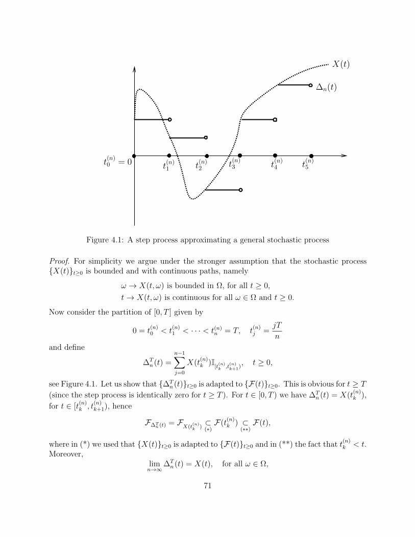
t(n)0 = 0 t

(n)1 t

(n)2

t(n)3 t

(n)4

X(t)

∆n(t)

t(n)5

Figure 4.1: A step process approximating a general stochastic process

Proof. For simplicity we argue under the stronger assumption that the stochastic processX(t)t≥0 is bounded and with continuous paths, namely

ω → X(t, ω) is bounded in Ω, for all t ≥ 0,

t→ X(t, ω) is continuous for all ω ∈ Ω and t ≥ 0.

Now consider the partition of [0, T ] given by

0 = t(n)0 < t

(n)1 < · · · < t(n)

n = T, t(n)j =

jT

n

and define

∆Tn (t) =

n−1∑j=0

X(t(n)k )I

[t(n)k ,t

(n)k+1)

, t ≥ 0,

see Figure 4.1. Let us show that ∆Tn (t)t≥0 is adapted to F(t)t≥0. This is obvious for t ≥ T

(since the step process is identically zero for t ≥ T ). For t ∈ [0, T ) we have ∆Tn (t) = X(t

(n)k ),

for t ∈ [t(n)k , t

(n)k+1), hence

F∆Tn (t) = F

X(t(n)k )⊂(∗)F(t

(n)k ) ⊂

(∗∗)F(t),

where in (*) we used that X(t)t≥0 is adapted to F(t)t≥0 and in (**) the fact that t(n)k < t.

Moreover,limn→∞

∆Tn (t) = X(t), for all ω ∈ Ω,

71

by the assumed continuity of the paths of X(t)t≥0. For the next step we use the dominatedconvergence theorem, see Remark 3.2. Since ∆T

n (t) and X(t) are bounded on [0, T ]×Ω, thereexists a constant CT such that |∆n(t)−X(t)|2 ≤ CT . Hence we may move the limit on theleft hand side of (4.4) across the expectation and integral operators and conclude that

limn→∞

E[

∫ T

0

|∆Tn (t)−X(t)|2 dt] = E[

∫ T

0

limn→∞

|∆Tn (t)−X(t)|2 dt] = 0,

as claimed.

4.3 Ito’s integral of general stochastic processes

The Ito integral of a general stochastic process is defined as the limit of the Ito integralalong a sequence of approximating step processes (in the sense of Theorem 4.2). The precisedefinition is the following.

Theorem 4.3 (and Definition). Let X(t)t≥0 ∈ L2[F(t)], T > 0 and ∆Tn (t)t≥0n∈N

be a sequence of L2[F(t)]-step processes converging to X(t)t≥0 in the sense of (4.4). Let

In(T ) =

∫ T

0

∆Tn (s)dW (s).

Then there exists a random variable I(T ) such that

‖In(T )− I(T )‖2 :=√E[|In(T )− I(T )|2]→ 0, as n→∞.

The random variable I(T ) is independent of the sequence of L2[F(t)]-step processes con-verging to X(t)t≥0. I(T ) is called Ito’s integral of X(t)t≥0 on the interval [0, T ] anddenoted by

I(T ) =

∫ T

0

X(s)dW (s).

Proof. By Ito’s isometry,

E[|In(T )− Im(T )|2] = E[

∫ T

0

|∆Tn (s)−∆T

m(s)|2ds].

We have

E[

∫ T

0

|∆Tn (s)−∆T

m(s)|2ds] ≤ 2E[

∫ T

0

|∆Tn (s)−X(s)|2ds]

+ 2E[

∫ T

0

|∆Tm(s)−X(s)|2ds]→ 0 as n,m→∞.

72

It follows that In(T )n∈N is a Cauchy sequence in the norm ‖ · ‖2. As mentioned in Re-mark 3.5, the norm ‖ · ‖2 is complete, i.e., Cauchy sequences converge. This proves the exis-tence of I(T ) such that ‖In(T )− I(T )‖2 → 0. To prove that the limit is the same along anysequence of L2[F(t)]-step processes converging to X(t)t≥0, assume that ∆n(t)t≥0n∈N,

∆n(t)t≥0n∈N are two such sequences and denote

In(T ) =

∫ T

0

∆n(s)dW (s), In(t) =

∫ T

0

∆n(s)dW (s).

Then, using (i), (iv) in Theorem 4.1, we compute

E[(In(T )− In(T ))2] = E[(

∫ T

0

(∆n(s)− ∆n(s))dW (s))2] = E[

∫ T

0

|∆n(s)− ∆n(s)|2ds]

≤ 2E[

∫ T

0

|∆n(s)−X(s)|2ds] + 2E[

∫ T

0

|∆n(s)−X(s)|2ds]→ 0,

as n→∞,

which proves that In(T ) and In(T ) have the same limit. This completes the proof of thetheorem.

As a way of example, we compute the Ito integral of the Brownian motion. We claim that,for all T > 0, ∫ T

0

W (t)dW (t) =W 2(T )

2− T

2. (4.5)

To prove the claim, we approximate the Brownian motion by the sequence of step processesintroduced in the proof of Theorem 4.2. Hence we define

∆Tn (t) =

n−1∑j=0

W (jT

n)I[ jT

n, j+1nT ).

By definition

In(T ) =

∫ T

0

∆Tn (t)dW (t) =

n−1∑j=0

W (jT

n)[W (

(j + 1)T

n)−W (

jT

n)].

To simplify the notation we let Wj = W (jT/n). Hence our goal is to prove

E[

∣∣∣∣∣n−1∑j=0

Wj(Wj+1 −Wj)−W 2(T )

2+T

2

∣∣∣∣∣2

]→ 0, as n→∞. (4.6)

We prove below that the sum within the expectation can be rewritten as

n−1∑j=0

Wj(Wj+1 −Wj) =1

2W (T )2 − 1

2

n−1∑j=0

(Wj+1 −Wj)2. (4.7)

73

Hence (4.6) is equivalent to

1

4E[

∣∣∣∣∣n−1∑j=0

(Wj+1 −Wj)2 − T

∣∣∣∣∣2

]→ 0, as n→∞,

which holds true by the already proven fact that [W,W ](T ) = T , see Theorem 3.9. It remainsto establish (4.7). Since W (T ) = Wn, we have

W (T )

2− 1

2

n−1∑j=0

(Wj+1 −Wj)2 =

1

2W 2n −

1

2

n−1∑j=0

W 2j+1 −

1

2

n−1∑j=0

W 2j +

n−1∑j=0

WjWj+1

= −1

2

n−2∑j=0

W 2j+1 −

1

2

n−1∑j=1

W 2j +

n−1∑j=1

WjWj+1

= −n−1∑j=1

W 2j +

n−1∑j=1

WjWj+1 =n−1∑j=1

Wj(Wj+1 −Wj)

=n−1∑j=0

Wj(Wj+1 −Wj).

The proof of (4.5) is complete.

Exercise 4.1 (?). Use the definition of Ito’s integral to prove that

TW (T ) =

∫ T

0

W (t)dt+

∫ T

0

tdW (t). (4.8)

The Ito integral can be defined under weaker assumptions on the integrand stochastic processthan those considered so far. As this fact will be important in the following sections, it isworth to briefly discuss it. LetM2 denote the set of F(t)t≥0-adapted stochastic processes

X(t)t≥0 such that∫ T

0X(t)2 dt is bounded a.s. for all T > 0 (of course, L2[F(t)] ⊂M2).

Theorem 4.4 (and Definition). For every process X(t)t≥0 ∈M2 and T > 0 there existsa sequence of step processes ∆T

n (t)t≥0n∈N ⊂M2 such that

limn→∞

∫ T

0

|X(s)−∆Tn (s)|2 ds→ 0 a.s.

and ∫ T

0

∆n(t)dW (t)

converges in probability as n→∞. The limit is independent of the sequence of step processesconverging to X(t)t≥0 and is called the Ito integral of the process X(t)t≥0 in the interval[0, T ]. If X(t)t≥0 ∈ L2[F(t)], the Ito integral just defined coincides (a.s.) with the onedefined in Theorem 4.3.

74

For the proof of the previous theorem, see [1, Sec. 4.4]. We remark that Theorem 4.4 impliesthat all F(t)t≥0-adapted stochastic processes with a.s. continuous paths are Ito integrable.In fact, if X(t)t≥0 has a.s. continuous paths, then for all T > 0, there exists CT (ω) suchthat supt∈[0,T ] |X(t, ω)| ≤ CT (ω) a.s. Hence∫ T

0

|X(s)|2 ds ≤ TC2T (ω), a.s.

and thus Theorem 4.4 applies. The case of stochastic processes with a.s. continuous pathscovers all the applications in the following chapters, hence we shall restrict to it from nowon.

Definition 4.2. We define C0[F(t)] to be the space of all F(t)t≥0-adapted stochastic pro-cesses X(t)t≥0 with a.s. continuous paths.

In particular, if X(t)t≥0, Y (t)t≥0 ∈ C0[F(t)], then for all continuous functions f theprocess f(t,X(t), Y (t))t≥0 belongs to C0[F(t)] and thus it is Ito integrable.

The properties listed in Theorem 4.1 carry over to the Ito integral of a general stochasticprocess. For easy reference, we rewrite these properties in the following theorem.

Theorem 4.5. Let X(t)t≥0 ∈ C0[F(t)]. Then the Ito integral

I(t) =

∫ t

0

X(s)dW (s) (4.9)

satisfies the following properties for all t ≥ 0.

(0) I(t)t≥0 ∈ C0[F(t)]. If X(t)t≥0 ∈ L2[F(t)], then I(t)t≥0 ∈ L2[F(t)].

(i) Linearity: For all stochastic processes X1(t)t≥0, X2(t)t≥0 ∈ C0[F(t)] and realconstants c1, c2 ∈ R there holds∫ t

0

(c1X1(s) + c2X2(s))dW (s) = c1

∫ t

0

X1(s)dW (s) + c2

∫ t

0

X2(s)dW (s).

(ii) Martingale property: If X(t)t≥0 ∈ L2[F(t)], the stochastic process I(t)t≥0 isa martingale in the filtration F(t)t≥0. In particular, E[I(t)] = E[I(0)] = 0, for allt ≥ 0.

(iii) Quadratic variation: For all T > 0, the quadratic variation of the stochastic processI(t)t≥0 on the interval [0, T ] is independent of the sequence of partitions along whichit is computed and it is given by

[I, I](T ) =

∫ T

0

X2(s) ds. (4.10)

75

(iv) Ito’s isometry: If X(t)t≥0 ∈ L2[F(t)], then Var[I(t)] = E[I2(t)] = E[∫ t

0X2(s) ds],

for all t ≥ 0.

(v) Martingale representation theorem: Let M(t)t≥0 ∈ L2[FW (t)] for all t ≥ 0, bea martingale stochastic process relative to the filtration FW (t)t≥0. Then there existsa stochastic process Γ(t)t≥0 ∈ L2[FW (t)] such that

M(t) = M(0) +

∫ t

0

Γ(s)dW (s), for all t ≥ 0.

Proof of (ii). By (iv) and the Schwartz inequality, E[I(t)] ≤√E[I2(t)] < ∞. According

to (3.20), it now suffices to show that

E[I(t)IA] = E[I(s)IA], for all A ∈ F(s).

Let In(t)t≥0n∈N be a sequence of Ito integrals of step processes which converges toI(t)t≥0 in L2(Ω), uniformly in compact intervals of time (see Theorem 4.3). Since In(t)t≥0

is a martingale for each n ∈ N, see Theorem 4.1, then

E[In(t)IA] = E[In(s)IA], for all A ∈ F(s).

Hence the claim follows if we show that E[In(t)IA] → E[I(t)IA], for all t ≥ 0. Using theSchwarz inequality (3.3), we have

E[(In(t)− I(t))IA] ≤√E[(In(t)− I(t))2]E[IA] ≤ ‖In(t)− I(t)‖2

√P(A)

≤ ‖In(t)− I(t)‖2 → 0, as n→∞,

and the claim follows.

Remark 4.1. Note carefully that the martingale property (ii) requires X(t)t≥0 ∈ L2[F(t)].A stochastic process in C0[F(t)] \ L2[F(t)] is not a martingale in general (although it is alocal martingale, see [1]).

Remark 4.2. For a proof of the martingale representation theorem see for instance Theorem4.3.4 in [21]. This important result will be used in Chapter 6 to show the existence of hedgingportfolios of European derivatives, see Theorem 6.2. Note carefully that the filtration used inthe martingale representation theorem must be the one generated by the Brownian motion.

Exercise 4.2. Prove the following generalization of Ito’s isometry. Let X(t)t≥0, Y (t)t≥0 ∈C0[F(t)]∩L2[F(t)] and denote by IX(t), IY (t) their Ito integral over the interval [0, t]. Then

Cov(IX(t), IY (t)) = E[

∫ t

0

X(s)Y (s) ds].

We conclude this section by introducing the “differential notation” for stochastic integrals.Instead of (4.9), we write

dI(t) = X(t)dW (t).

76

For instance, the identities (4.5), (4.8) are also expressed as

d(W 2(t)) = dt+ 2W (t)dW (t), d(tW (t)) = W (t)dt+ tdW (t).

The quadratic variation (4.10) is expressed also as

dI(t)dI(t) = X2(t)dt.

Note that this notation is in agreement with the one already introduced in Section 3.2,namely

dI(t)dI(t) = d

(∫ t

0

X2(s)ds

)= X2(t)dt.

The differential notation is very useful to provide informal proofs in stochastic calculus.For instance, using dI(t) = X(t)dW (t), and dW (t)dW (t) = dt, see (3.12), we obtain thefollowing simple “proof” of Theorem 4.5(iii):

dI(t)dI(t) = X(t)dW (t)X(t)dW (t) = X2(t)dW (t)dW (t) = X2(t)dt.

4.4 Diffusion processes

Now that we know how to integrate along the paths of a Brownian motion, we can define anew class of stochastic processes.

Definition 4.3. Given α(t)t≥0, σ(t)t≥0 ∈ C0[F(t)], the stochastic process X(t)t≥0 ∈C0[F(t)] given by

X(t) = X(0) +

∫ t

0

σ(s)dW (s) +

∫ t

0

α(s) ds, t ≥ 0 (4.11)

is called diffusion process (or Ito process) with diffusion σ(t)t≥0 and drift α(t)t≥0.

We denote diffusion processes also as

dX(t) = σ(t)dW (t) + α(t)dt. (4.12)

Note that

dX(t)dX(t) = σ2(t)dW (t)dW (t) + α2(t)dtdt+ σ(t)α(t)dW (t)dt

and thus, by (3.11), (3.12) and (3.14), we obtain

dX(t)dX(t) = σ2(t)dt,

which means that the quadratic variation of the diffusion process (4.12) is given by

[X,X](t) =

∫ t

0

σ2(s) ds, t ≥ 0.

77

Thus the squared of the diffusion term in a diffusion process is the rate of quadratic variationof the diffusion process. Furthermore, assuming σ(t)t≥0 ∈ L2[F(t)], we have

E[

∫ t

0

σ(s)dW (s)] = 0.

Hence the term∫ t

0α(s)ds is the only one contributing to the evolution of the average of

X(t)t≥0, which is the reason to call α(t) the drift of the diffusion process (if α = 0 andσ(t)t≥0 ∈ L2[F(t)], the diffusion process is a martingale, as it follows by Theorem 4.5(ii)).Finally, the integration along the paths of the diffusion process (4.12) is defined as∫ t

0

Y (s)dX(s) :=

∫ t

0

Y (s)σ(s)dW (s) +

∫ t

0

Y (s)α(s)ds, (4.13)

for all Y (t)t≥0 ∈ C0[F(t)].

The product rule in stochastic calculus

Recall that if f, g : R→ R are two differentiable functions, the product (or Leibnitz) rule ofordinary calculus states that

(fg)′ = f ′g + fg′,

and thus

fg(t) = fg(0) +

∫ t

0

(g(s)df(s) + f(s)dg(s)).

Can this rule be true in stochastic calculus, i.e., when f and g are general diffusion processes?The answer is clearly no. In fact, letting for instance f(t) = g(t) = W (t), Leibnitz’s rule giveus the relation d(W 2(t)) = 2W (t)dW (t), while we have seen before that the correct formulain Ito’s calculus is d(W 2(t)) = 2W (t)dW (t) + t. The correct product rule in Ito’s calculus isthe following.

Theorem 4.6. Let X1(t)t≥0 and X2(t)t≥0 be the diffusion processes

dXi(t) = σi(t)dW (t) + θi(t)dt.

Then X1(t)X2(t)t≥0 is the diffusion process given by

d(X1(t)X2(t)) = X2(t)dX1(t) +X1(t)dX2(t) + σ1(t)σ2(t)dt. (4.14)

Exercise 4.3 (Sol. 23). Prove the theorem in the case that αi and σi are deterministicconstants and Xi(0) = 0, for i = 1, 2.

Recall that the correct way to interpret (4.14) is

X1(t)X2(t) = X1(0)X2(0) +

∫ t

0

X2(s)dX1(s) +

∫ t

0

X1(s)dX2(s) +

∫ t

0

σ1(s)σ2(s)ds, (4.15)

78

where the integrals along the paths of the processes Xi(t)t≥0 are defined as in (4.13). Notethat all integrals in (4.15) are well-defined, since the integrand stochastic processes have a.s.continuous paths. We also remark that, since

dX1(t)dX2(t) = (σ1(t)dW (t) + α1(t)dt)(σ2(t)dW (t) + α2(t)dt)

= σ1(t)σ2(t)dW (t)dW (t) + (α1(t)σ2(t) + α2(t)σ1(t))dW (t)dt+ α1(t)α2(t)dtdt

= σ1(t)σ2(t)dt,

then we may rewrite (4.14) as

d(X1(t)X2(t)) = X2(t)dX1(t) +X1(t)dX2(t) + dX1(t)dX2(t), (4.16)

which is somehow easier to remember. Going back to the examples considered in Section 4.3,the Ito product rule gives

d(W 2(t)) = W (t)dW (t) +W (t)dW (t) + dW (t)dW (t) = 2W (t)dW (t) + dt,

d(tW (t)) = tdW (t) +W (t)dt+ dW (t)dt = tdW (t) +W (t)dt,

in agreement with our previous calculations, see (4.5) and (4.8).

The chain rule in stochastic calculus

Next we consider the generalization to Ito’s calculus of the chain rule. Let us first recall howthe chain rule works in ordinary calculus. Assume that f : R × R → R and g : R → R aredifferentiable functions. Then

d

dtf(t, g(t)) = ∂tf(t, g(t)) + ∂xf(t, g(t))

d

dtg(t),

by which we derive

f(t, g(t)) = f(0, g(0)) +

∫ t

0

∂sf(s, g(s)) ds+

∫ t

0

∂xf(s, g(s)) dg(s).

Can this formula be true in stochastic calculus, i.e., when g is a diffusion process? Theanswer is clearly no. In fact by setting f(t, x) = x2, g(t) = W (t) and t = T in the previousformula we obtain

W 2(T ) = 2

∫ T

0

W (t)dW (t), i.e.,

∫ T

0

W (t)dW (t) =W 2(T )

2,

while the Ito integral of the Brownian motion is given by (4.5). The correct formula for thechain rule in stochastic calculus is given in the following theorem.

Theorem 4.7. Let f : R×R→ R, f = f(t, x), be a C1 function such that ∂2xf is continuous

79

and let X(t)t≥0 be the diffusion process dX(t) = σ(t)dW (t) +α(t)dt. Then Ito’s formulaholds:

df(t,X(t)) = ∂tf(t,X(t)) dt+ ∂xf(t,X(t)) dX(t) +1

2∂2xf(t,X(t)) dX(t)dX(t), (4.17)

i.e.,

df(t,X(t)) = ∂tf(t,X(t)) dt+ ∂xf(t,X(t)) (σ(t)dW (t) + α(t)dt) +1

2∂2xf(t,X(t))σ2(t) dt.

(4.18)

For instance, letting X(t) = W (t) and f(t, x) = x2, we obtain d(W 2(t)) = 2W (t)dW (t) +dt,i.e., (4.5), while for f(t, x) = tx we obtain d(tW (t)) = W (t)dt + tdW (t), which is (4.8). Infact, the proof of Theorem 4.7 is similar to proof of (4.5) and (4.8). We omit the details(see [25, Theorem 4.4.1] for a sketch of the proof).

Recall that (4.18) is a shorthand for

f(t,X(t)) = f(0, X(0))+

∫ t

0

(∂tf+α(s)∂xf+1

2σ2(s)∂2

xf)(s,X(s)) ds+

∫ t

0

∂xf(s,X(s))dW (s).

All integrals in the right hand side of the previous equation are well defined, as the integrandstochastic processes have continuous paths. We conclude with the generalization of Ito’sformula to functions of several random variables, which again we give without proof.

Theorem 4.8. Let f : R × RN → R be a C1 function such that f = f(t, x) is twice con-tinuously differentiable on the variable x ∈ RN . Let X1(t)t≥0, . . . , XN(t)t≥0 be diffusionprocesses and let X(t) = (X1(t), . . . , XN(t)). Then there holds:

df(t,X(t)) = ∂tf(t,X(t)) dt+N∑i=1

∂xif(t,X(t)) dXi(t)

+1

2

N∑i,j=1

∂xi∂xjf(t,X(t)) dXi(t)dXj(t). (4.19)

For instance, for N = 2 and letting f(t, x1, x2) = x1x2 into (4.19), we obtain the Ito productrule (4.16).

Remark 4.3. Let X(t)t≥0, Y (t)t≥0 be diffusion processes and define the complex-valuedstochastic process Z(t)t≥0 by Z(t) = X(t) + iY (t). Then any stochastic process of theform g(t, Z(t)) can be written in the form f(t,X(t), Y (t)), where f(t, x, y) = g(t, x + iy).Hence dg(t, Z(t)) can be computed using Theorem 4.8. An application to this formula isgiven in Exercise 4.8 below.

The following exercises help to get familiar with the rules of stochastic calculus.

80

Exercise 4.4 (Sol. 24). Let W1(t)t≥0, W2(t)t≥0 be Brownian motions. Assume that thereexists a constant ρ ∈ [−1, 1] such that dW1(t)dW2(t) = ρdt. Show that ρ is the correlation ofthe two Brownian motions at time t. Assuming that W1(t)t≥0, W2(t)t≥0 are independent,compute P(W1(t) > W2(s)), for all s, t > 0.

Exercise 4.5 (Sol. 25). Consider the stochastic process X(t)t≥0 defined by X(t) = W (t)3−3tW (t). Show that X(t)t≥0 is a martingale and find a process Γ(t)t≥0 adapted toFW (t)t≥0 such that

X(t) = X(0) +

∫ t

0

Γ(s)dW (s).

(The existence of the process Γ(t)t≥0 is ensured by Theorem 4.5(v).)

Exercise 4.6 (Sol. 26). Let θ(t)t≥0 ∈ C0[F(t)] and define the stochastic process Z(t)t≥0

by

Z(t) = exp

(−∫ t

0

θ(s)dW (s)− 1

2

∫ t

0

θ2(s)ds

).

Show that

Z(t) = 1−∫ t

0

θ(s)Z(s) dW (s).

Processes of the form considered in Exercise 4.6 are fundamental in mathematical finance.In particular, it is important to know whether Z(t)t≥0 is a martingale. By Exercise 4.6 andTheorem 4.5(ii), Z(t)t≥0 is a martingale if θ(t)Z(t) ∈ L2[F(t)], which is however difficultin general to verify directly. The following condition, known as Novikov’s condition, ismore useful in the applications, as it involves only the time-integral of the process θ(t)t≥0.The proof can be found in [16].

Theorem 4.9. Let θ(t)t≥0 ∈ C0[F(t)] satisfy

E[exp(1

2

∫ T

0

θ(t)2 dt)] <∞, for all T > 0. (4.20)

Then the stochastic process Z(t)t≥0 given by

Z(t) = exp

(−∫ t

0

θ(s)dW (s)− 1

2

∫ t

0

θ2(s)ds

).

is a martingale relative the filtration F(t)t≥0.

In particular, the stochastic process Z(t)t≥0 is a martingale when θ(t) = const, hence werecover the result of Exercise 3.29. The following exercise extends the result of Exercise 4.6to the case of several independent Brownian motions.

Exercise 4.7. Let W1(t)t≥0, . . . , WN(t)t≥0 be independent Brownian motions and let

81

F(t)t≥0 be a non-anticipating filtration for all of them. Let θ1(t)t≥0, . . . θN(t)t≥0 ∈C0[F(t)] be adapted to F(t)t≥0 and set θ(t) = (θ1(t), . . . , θN(t)). Compute dZ(t), where

Z(t) = exp

(−

N∑j=1

∫ t

0

θj(s)dWj(s)−1

2

∫ t

0

‖θ(s)‖2ds

),

where ‖θ(t)‖ =√θ1(t)2 + · · ·+ θN(t)2 is the Euclidean norm of θ(t).

Exercise 4.8 (Sol. 27). Let A : R→ R be continuous deterministic function of time. Showthat the random variable

I(t) =

∫ t

0

A(s) dW (s)

is normally distributed with zero expectation and variance∫ t

0A(s)2ds.

Exercise 4.9. Show that the process W 2(t) − tt≥0 is a martingale relative to F(t)t≥0,where W (t)t≥0 is a Brownian motion and F(t)t≥0 a non-anticipating filtration thereof.Prove also the following logically opposite statement: assume that X(t)t≥0 and X2(t) −tt≥0 are martingales relative to F(t)t≥0, X(t)t≥0 has a.s. continuous paths and X(0) =0 a.s.. Then X(t)t≥0 is a Brownian motion with non-anticipating filtration F(t)t≥0.

4.5 Girsanov’s theorem

In this section we assume that the non-anticipating filtration of the Brownian motion coin-cides with FW (t)t≥0. Let θ(t)t≥0 ∈ C0[FW (t)] satisfy the Novikov condition (4.20). Itfollows by Theorem 4.9 that the positive stochastic process Z(t)t≥0 given by

Z(t) = exp

(−∫ t

0

θ(s)dW (s)− 1

2

∫ t

0

θ2(s)ds

)(4.21)

is a martingale relative to FW (t)t≥0. As Z(0) = 1, then E[Z(t)] = 1 for all t ≥ 0. Thus

we can use the stochastic process Z(t)t≥0 to generate a measure P equivalent to P as we

did at the end of Section 3.4, namely P : F → [0, 1] is given by

P(A) = E[Z(T )IA], A ∈ F , (4.22)

for some given T > 0. The relation between E and E has been determined in Theorem 3.18,where we showed that

E[X] = E[Z(t)X], (4.23)

for all t ≥ 0 and FW (t)-measurable random variables X, and

E[Y |FW (s)] =1

Z(s)E[Z(t)Y |FW (s)] (4.24)

for all 0 ≤ s ≤ t and random variables Y . We can now state and sketch the proof ofGirsanov’s theorem, which is a fundamental result with deep applications in mathematicalfinance.

82

Theorem 4.10. Define the stochastic process W (t)t≥0 by

W (t) = W (t) +

∫ t

0

θ(s)ds, (4.25)

i.e., dW (t) = dW (t)+θ(t)dt. Then W (t)t≥0 is a P-Brownian motion. Moreover FW (t)t≥0

is a non-anticipating filtration for the P-Brownian motion W (t)t≥0.

Sketch of the proof. We prove the theorem using the Levy characterization of Brownian mo-tions, see Theorem 3.17. Clearly, W (t)t≥0 starts from zero and has continuous paths a.s.

Moreover we (formally) have dW (t)dW (t) = dW (t)dW (t) = dt. Hence it remains to show

that the Brownian motion W (t)t≥0 is P-martingale relative to the filtration FW (t)t≥0.By Ito’s product rule we have

d(W (t)Z(t)) = W (t)dZ(t) + Z(t)dW (s) + dW (t)dZ(t)

= (1− θ(t)W (t))Z(t)dW (t),

that is to say,

W (t)Z(t) =

∫ t

0

(1− W (u)θ(u))Z(u)dW (u).

It follows by Theorem 4.5(ii) that the stochastic process Z(t)W (t)t≥0 is a P-martingalerelative to FW (t)t≥0, i.e.,

E[Z(t)W (t)|FW (s)] = Z(s)W (s).

But according to (4.24),

E[Z(t)W (t)|FW (s)] = Z(s)E[W (t)|FW (s)].

Hence E[W (t)|FW (s)] = W (s), as claimed.

Later we shall need also the multi-dimensional version of Girsanov’s theorem. Let

W1(t)t≥0, . . . , WN(t)t≥0

be independent Brownian motions and let FW (t)t≥0 be their own generated filtration. Letθ1(t)t≥0, . . . , θN(t)t≥0 ∈ C0[FW (t)] and set θ(t) = (θ1(t), . . . , θN(t)). We assume that theNovikov condition (4.20) is satisfied (with θ(t)2 = ‖θ(t)‖2 = θ1(t)2 + · · ·+ θN(t)2). Then, asshown in Exercise 4.7, the stochastic process Z(t)t≥0 given by

Z(t) = exp

(−

N∑j=1

∫ t

0

θj(s)dWj(s)−1

2

∫ t

0

‖θ(s)‖2ds

)

83

is a martingale relative to FW (t)t≥0. It follows as before that the map P : F → [0, 1] givenby

P(A) = E[Z(T )IA], A ∈ F (4.26)

is a new probability measure equivalent to P and the following N -dimensional generalizationof Girsanov’s theorem holds.

Theorem 4.11. Define the stochastic processes W1(t)t≥0, . . . , WN(t)t≥0 by

Wk(t) = Wk(t) +

∫ t

0

θk(s)ds, k = 1, . . . , N. (4.27)

Then W1(t)t≥0, . . . , WN(t)t≥0 are independent Brownian motions in the probability mea-

sure P. Moreover the filtration FW (t)t≥0 generated by W1(t)t≥0, . . . , WN(t)t≥0 is a

non-anticipating filtration for W1(t)t≥0, . . . , WN(t)t≥0.

4.6 Diffusion processes in financial mathematics

The purpose of this final section is to introduce some important examples of diffusion pro-cesses in financial mathematics. The analysis of the properties of such processes is the subjectof Chapter 6.

Generalized geometric Brownian motion

Given two stochastic processes α(t)t≥0, σ(t)t≥0 ∈ C0[FW (t)], the stochastic processS(t)t≥0 ∈ C0[FW (t)] given by

S(t) = S(0) exp

(∫ t

0

α(s)ds+

∫ t

0

σ(s)dW (s)

)is called generalized geometric Brownian motion with instantaneous mean of log-return α(t)t≥0 and instantaneous volatility σ(t)t≥0. When α(t) = α ∈ R andσ(t) = σ > 0 are deterministic constant, the process above reduces to the geometric Brownianmotion, see (2.14). The generalized geometric Brownian motion provides a quite more generaland realistic model for the dynamics of stock prices than the simple geometric Brownianmotion. In the rest of these notes we assume that stock prices are modeled by generalizedgeometric Brownian motions.

SinceS(t) = S(0)eX(t), dX(t) = α(t)dt+ σ(t)dW (t),

84

then Ito’s formula gives

dS(t) = S(0)eX(t)dX(t) +1

2S(0)eX(t)dX(t)dX(t)

= S(t)α(t)dt+ S(t)σ(t)dW (s) +1

2σ2(t)S(t)dt

= µ(t)S(t)dt+ σ(t)S(t)dW (t), where µ(t) = α(t) +1

2σ2(t),

hence a generalized geometric Brownian motion is a diffusion process in which the diffusionand the drift depend on the process itself.

In the presence of several stocks, it is reasonable to assume that each of them introduced anew source of randomness in the market. Thus, when dealing with N stocks, we assume theexistence of N independent Brownian motions W1(t)t≥0, . . . , WN(t)t≥0 and model theevolution of the stocks prices S1(t)t≥0, . . . , SN(t)t≥0 by the following N-dimensionalgeneralized geometric Brownian motion:

dSk(t) =

(µk(t) +

N∑j=1

σkj(t)dWj(t)

)Sk(t) (4.28)

for some stochastic processes µk(t)t≥0, σkj(t)t≥0 ∈ C0[FW (t)], j, k = 1, . . . , N .

Self-financing portfolios

Consider a portfolio hS(t), hB(t)t≥0 invested in a 1+1-dimensional market. We assumethat the price of the stock follows the generalized geometric Brownian motion

dS(t) = µ(t)S(t)dt+ σ(t)S(t)dW (t), (4.29)

while the value of the risk-free asset is given by (2.15), i.e.,

dB(t) = B(t)R(t)dt, (4.30)

where R(t)t≥0 is the risk-free rate of the money market. Moreover we assume that themarket parameters µ(t)t≥0, σ(t)t≥0, R(t)t≥0 have continuous paths a.s. and areadapted to the filtration FW (t)t≥0. The value of the portfolio is given by

V (t) = hS(t)S(t) + hB(t)B(t). (4.31)

We say that the portfolio is self-financing if purchasing more shares of one asset is possibleonly by selling shares of the other asset for an equivalent value (and not by infusing new cashinto the portfolio), and, conversely, if any cash obtained by selling one asset is immediatelyre-invested to buy shares of the other asset (and not withdrawn from the portfolio). Totranslate this condition into a mathematical formula, assume that (hS, hB) is the investor

85

position on the stock and the risk-free asset during the “infinitesimal” time interval [t, t+δt).Let V −(t+ δt) be the value of this portfolio immediately before the time t+ δt at which theposition is changed, i.e.,

V −(t+ δt) = limu→t+δt

hSS(u) + hBB(u) = hSS(t+ δt) + hBB(t+ δt),

where we used the continuity in time of the assets price. At the time t + δt, the investorsells/buys shares of the assets. Let (h′S, h

′B) be the new position on the stock and the risk-free

asset. Then the value of the portfolio at time t+ δt is given by

V (t+ δt) = h′SS(t+ δt) + h′BB(t+ δt).

The difference V (t + δt)− V −(t + δt), if not zero, corresponds to cash withdrawn or addedto the portfolio as a result of the change in the position on the assets. In a self-financingportfolio, however, this difference must be zero. We obtain

V (t+ δt)− V −(t+ δt) = 0⇔ (hS − h′S)S(t+ δt) + (hB − h′B)B(t+ δt) = 0.

Hence, the change of the portfolio value in the interval [t, t+ δt] is given by

δV = V (t+ δt)− V (t) = h′SS(t+ δt) + h′BB(t+ δt)− (hSS(t) + hBB(t)) = hSδS + hBδB,

where δS = S(t+ δt)− S(t), and δB = B(t+ δt)−B(t) are the changes of the assets valuein the interval [t, t+ δt]. This discussion leads to the following definition.

Definition 4.4. A portfolio process hS(t), hB(t)t≥0 invested in the 1+1-dimensional mar-ket (4.29)-(4.30) is said to be self-financing if it is adapted to FW (t)t≥0 and if its valueprocess V (t)t≥0 satisfies

dV (t) = hS(t)dS(t) + hB(t)dB(t). (4.32)

Exercise 4.10 (Sol. 28). Show that given a diffusion process hS(t)t≥0, it is always possibleto find a diffusion process hB(t)t≥0 such that the portfolio process hS(t), hB(t)t≥0 is self-financing.

We conclude with the important definition of hedging portfolio. Suppose that at time t aEuropean derivative with pay-off Y at the time of maturity T > t is sold for the price ΠY (t).An important problem in financial mathematics is to find a strategy for how the seller shouldinvest the premium ΠY (t) of the derivative in order to hedge the derivative, i.e., in order toensure that the portfolio value of the seller at time T is enough to pay-off the buyer of thederivative. We assume that the seller invests the premium of the derivative only on the 1+1dimensional market consisting of the underlying stock and the risk-free asset (∆-hedging).

Definition 4.5. Consider the European derivative with pay-off Y and time of maturity T ,where we assume that Y is FW (T )-measurable. A portfolio process hS(t), hB(t)t≥0 investedin the underlying stock and the risk-free asset is said to be an hedging portfolio if

86

(i) hS(t), hB(t)t≥0 is adapted to FW (t)t≥0;

(ii) The value of the portfolio satisfies V (T ) = Y .

In Chapter 6 we shall answer the following questions:

1) What is a reasonable “fair” price for the European derivative at time t ∈ [0, T ] ?

2) What investment strategy (on the underlying stock and the risk-free asset) should theseller undertake in order to hedge the derivative?

87

Chapter 5

Stochastic differential equations andpartial differential equations

Throughout this chapter, the probability space (Ω,F ,P) is given and F(t)t≥0 denotes anon-anticipating filtration for the given Brownian motion W (t)t≥0 (e.g., F(t) ≡ FW (t)).Given T > 0, we denote by DT the open region in the (t, x)-plane given by

DT = t ∈ (0, T ), x ∈ R = (0, T )× R.

The closure and the boundary of DT are given respectively by

DT = [0, T ]× R, ∂DT = t = 0, x ∈ R ∪ t = T, x ∈ R.Similarly we denote D+

T the open region

D+T = t ∈ (0, T ), x > 0 = (0, T )× (0,∞),

whose closure and boundary are given by

D+T = [0, T ]× [0,∞), ∂D+

T = t = 0, x ≥ 0 ∪ t = T, x ≥ 0 ∪ t ∈ [0, T ], x = 0.Moreover we shall employ the following notation for functions spaces: For D = DT or D+

T ,

• Ck(D) is the space of k-times continuously differentiable functions u : D → R;

• C1,2(D) is the space of functions u ∈ C1(D) such that ∂2xu ∈ C(D);

• Ck(D) is the space of functions u : D → R such that u ∈ Ck(D) and the partialderivatives of u up to order k extend continuously on D.

• Ckc (Rn) is the space k-times continuously differentiable functions u : Rn → R with

compact support. We also let C∞c (Rn) = ∩k∈NCkc (Rn)

A function u : D → R is uniformly bounded if there exists CT > 0 such that |u(t, x)| ≤ CT ,for all (t, x) ∈ D. Unless otherwise stated, all functions are real-valued.

88

5.1 Stochastic differential equations

Definition 5.1. Given s ≥ 0, α, β ∈ C0([s,∞) × R), and a deterministic constant x ∈ R,we say that a stochastic process X(t)t≥s is a global (strong) solution to the stochasticdifferential equation (SDE)

dX(t) = α(t,X(t)) dt+ β(t,X(t)) dW (t) (5.1)

with initial value X(s, ω) = x at time t = s, if X(t)t≥s ∈ C0[F(t)] and

X(t) = x+

∫ t

s

α(τ,X(τ)) dτ +

∫ t

s

β(τ,X(τ)) dW (τ), t ≥ s. (5.2)

The initial value of a SDE can be a random variable instead of a deterministic constant, butwe shall not need this more general case. Note also that the integrals in the right hand sideof (5.2) are well-defined, as the integrand functions have continuous paths a.s. Of courseone needs suitable assumptions on the functions α, β to ensure that there is a (unique)process X(t)t≥s satisfying (5.2). The precise statement is contained in the following globalexistence and uniqueness theorem for SDE’s, which is reminiscent of the analogous result forordinary differential equations (Picard’s theorem).

Theorem 5.1. Assume that for each T > s there exist constants CT , DT > 0 such that α, βsatisfy

|α(t, x)|+ |β(t, x)| ≤ CT (1 + |x|), (5.3)

|α(t, x)− α(t, y)|+ |β(t, x)− β(t, y)| ≤ DT |x− y|, (5.4)

for all t ∈ [s, T ], x, y ∈ R. Then there exists a unique global solution X(t)t≥s of theSDE (5.1) with initial value X(s) = x. Moreover X(t)t≥s ∈ L2[F(t)].

A proof of Theorem 5.1 can be found in [21, Theorem 5.2.1]. Note that the result provedin [21] is a bit more general than the one stated above, as it covers the case of systems ofSDE’s with random initial value.

The solution of (5.1) with initial initial value x at time t = s will be also denoted byX(t; s, x)t≥s. It can be shown that, under the assumptions of Theorem 5.1, the randomvariable X(t; s, x) depends (a.s.) continuously on the initial conditions (s, x), see [1, Sec. 7.3].

Remark 5.1. The uniqueness statement in Theorem 5.1 is to be understood “up to nullsets”. Precisely, if Xi(t)t≥s, i = 1, 2 are two solutions with the same initial value x, then

P( supt∈[s,T ]

|X1(t)−X2(t)| > 0) = 0, for all T > s.

Remark 5.2. If the assumptions of Theorem 5.1 are satisfied only up to a fixed time T > 0,then the solution of (5.1) could explode at some finite time in the future of T . For example,

89

the stochastic process given by X(t) = log(W (t) + ex) solves (5.1) with α = − exp(−2x)/2and β = exp(−x), but only up to the time T∗ = inft : W (t) = −ex > 0. Note that T∗is a random variable in the latter example1. In these notes we are only interested in globalsolutions of SDE’s, hence we require (5.3)-(5.4) to hold for all T > 0.

Remark 5.3. The growth condition (5.3) alone is sufficient to prove the existence of a globalsolution to (5.1). The Lipschitz condition (5.4) is used to ensure uniqueness. By using amore general notion of solution (weak solution) and uniqueness (pathwise uniqueness),one can extend Theorem 5.1 to a larger class of SDE’s, which include in particular the CIRprocess considered in Section 5.3; see [23] for details.

Exercise 5.1. Within many applications in finance, the drift term α(t, x) is linear, an so itcan be written in the form

α(t, x) = a(b− x), a, b constant. (5.5)

A stochastic process X(t)t≥0 is called mean reverting if there exists a constant c suchthat E[X(t)] → c as t → +∞. Most financial variables are required to satisfy the meanreversion property. Prove that the solution X(t; s, x)t≥0 of (5.1) with linear drift (5.5)satisfies

E[X(t; s, x)] = xe−a(t−s) + b(1− e−a(t−s)). (5.6)

Hence the process X(t; s, x)t≥0 is mean reverting if and only if a > 0 and in this case thelong time mean is given by c = b.

Linear SDE’s

A SDE of the form

dX(t) = (a(t) + b(t)X(t)) dt+ (γ(t) + σ(t)X(t)) dW (t), X(s) = x, (5.7)

where a, b, γ, σ are deterministic functions of time, is called a linear stochastic differentialequation. We assume that for all T > 0 there exists a constant CT such that

supt∈[s,T ]

(|a(t)|+ |b(t)|+ |γ(t)|+ |σ(t)|) < CT ,

and so by Theorem 5.1 there exists a unique global solution of (5.7). For example, thegeometric Brownian motion (2.14) solves the linear SDE dS(t) = µS(t) dt + σS(t) dW (t),where µ = α + σ2/2. Another example of linear SDE in finance is the Vasicek interest ratemodel, see Exercise 6.32. Linear SDE’s can be solved explicitly, as shown in the followingtheorem.

Theorem 5.2. The solution X(t)t≥s of (5.7) is given by X(t) = Y (t)Z(t), where

Z(t) = exp

(∫ t

s

σ(τ)dW (τ) +

∫ t

s

(b(τ)− σ(τ)2

2)dτ

),

1More precisely, a stopping time, see Definition 6.10.

90

Y (t) = x+

∫ t

s

a(τ)− σ(τ)γ(τ)

Z(τ)dτ +

∫ t

s

γ(τ)

Z(τ)dW (τ).

Exercise 5.2 (?). Proof Theorem 5.2.

For example, in the special case in which the functions a, b, γ, σ are constant (independentof time), the solution of (5.7) with initial value X(0) = x at time t = 0 is

X(t) = eσW (t)+(b−σ2

2)t(x+ (a− γσ)

∫ t

0

e−σW (τ)−(b−σ2

2)τdτ + γ

∫ t

0

e−σW (τ)−(b−σ2

2)τdW (τ)

).

Exercise 5.3 (Sol. 29). Consider the linear SDE (5.7) with constant coefficients a, b, γ andσ = 0. Find the solution and show that X(t; s, x) ∈ N (m(t− s, x),∆(t− s)2), where

m(τ, x) = xebτ +a

b(ebτ − 1), ∆(τ)2 =

γ2

2b(e2bτ − 1). (5.8)

Exercise 5.4 (Sol. 30). Find the solution X(t)t≥0 of the linear SDE

dX(t) = tX(t) dt+ dW (t), t ≥ 0

with initial value X(0) = 1. Find Cov(X(s), X(t)).

Exercise 5.5. Compute Cov(W (t), X(t)) and Cov(W 2(t), X(t)), where X(t) = X(t; s, x) isthe stochastic process in Exercise 5.3.

Markov property

It can be shown that, under the assumptions of Theorem 5.1, the solution X(t; s, x)t≥sof (5.1) is a Markov process, see for instance [1, Th. 9.2.3]. Moreover when α, β in (5.1) aretime-independent, X(t; s, x)t≥s is a homogeneous Markov process. The fact that solutionsof SDE’s should satisfy the Markov property is quite intuitive, for, as shown in Theorem 5.1,the solution at time t is uniquely characterized by the initial value at time s < t. Considerfor example the linear SDE

dX(t) = (a+ bX(t)) dt+ γdW (t), t ≥ s, X(s) = x. (5.9)

As shown in Exercise 5.5, the solution of (5.9) is given by

X(t; s, x) = xeb(t−s) +a

b(eb(t−s) − 1) +

∫ t

s

γeb(t−u)dW (u), t ≥ s,

and therefore X(t; s, x) ∈ N (m(t − s, x),∆(t − s)2), where m(τ, x) and ∆(τ) are givenby (5.8). By Theorem 3.19, the transition density of the Markov process X(t; s, x)t≥0 isgiven by the pdf of the random variable X(t; s, x), that is p(t, s, x, y) = p∗(t− s, x, y), where

p∗(τ, x, y) = e(y−m(τ,x))2

2∆(τ)21√

2π∆(τ)2. (5.10)

The previous example rises the question of whether the Markov process solution of SDE’salways admits a transition density. This problem is one of the subjects of Section 5.2.

91

Systems of SDE’s

Occasionally in the next chapter we need to consider systems of several SDE’s. All theresults presented in this section extend mutatis mutandis to systems of SDE’s, the differencebeing merely notational. For example, given two Brownian motions W1(t)t≥0, W2(t)t≥0

and continuous functions α1, α2, β11, β12, β21, β22 : [s,∞)× R2 → R, the relations

dXi(t) = αi(t,X1(t), X2(t)) dt+∑j=1,2

βij(t,X1(t), X2(t))dWj(t), (5.11a)

Xi(s) = xi, i = 1, 2 (5.11b)

define a system of two SDE’s on the stochastic processes X1(t)t≥0, X2(t)t≥0 with initialvalues X1(s) = x1, X2(s) = x2 at time s. As usual, the correct way to interpret the relationsabove is in the integral form:

Xi(t) = xi +

∫ t

s

αi(τ,X1(τ), X2(τ)) dτ +∑j=1,2

∫ t

s

βij(τ,X1(τ), X2(τ))dWj(τ) i = 1, 2.

Upon defining the vector and matrix valued functions α = (α1, α2)T , β = (βij)i,j=1,2, andletting X(t) = (X1(t), X2(t)), x = (x1, x2), W (t) = (W1(t),W2(t)), we can rewrite (5.11) as

dX(t) = α(t,X(t)) dt+ β(t,X(t)) · dW (t), X(s) = x, (5.12)

where · denotes the row by column matrix product. In fact, every system of any arbitrarynumber of SDE’s can be written in the form (5.12). Theorem 5.1 continues to be valid forsystems of SDE’s, the only difference being that |α|, |β| in (5.3)-(5.4) stand now for thevector norm of α and for the matrix norm of β.

5.2 Kolmogorov equations

Most financial variables are represented by stochastic processes solving (systems of) SDE’s.In this context, a problem which recurs often is to find a function f such that the processY (t)t≥0 given by Y (t) = f(t,X(t)) is a martingale, where X(t)t≥0 is the global solutionof (5.1) with initial value X(0) = x. To this regard we have the following result.

Theorem 5.3. Let T > 0 and u : DT → R such that u ∈ C1,2(DT ) and ∂xu is uniformlybounded. Assume that u satisfies

∂tu+ α(t, x)∂xu+1

2β(t, x)2∂2

xu = 0 (5.13)

in the region DT . Assume also that α, β satisfy the conditions in Theorem 5.1 (with s = 0)and let X(t)t≥0 be the unique global solution of (5.1) with initial value X(0) = x. Thestochastic process u(t,X(t))t∈[0,T ] is a martingale and satisfies

u(t,X(t)) = u(0, x) +

∫ t

0

β(τ,X(τ))∂xu(τ,X(τ)) dW (τ), t ∈ [0, T ]. (5.14)

92

Proof. By Ito’s formula we find

du(t,X(t)) = (∂tu+ α∂xu+β2

2∂2xu)(t,X(t)) dt+ (β∂xu)(t,X(t)) dW (t).

As u solves (5.13), then du(t,X(t)) = (β∂xu)(t,X(t)) dW (t), which is equivalent to (5.14)(because u(0, X(0)) = u(0, x)). As ∂xu is uniformly bounded, there exists a constant CT > 0such that |∂xu(t, x)| ≤ CT and so, due also to (5.3), the process Y (t) = β∂xu(t,X(t)) satisfies|Y (t)| ≤ CT (1 + |X(t)|). Since X(t)t≥0 ∈ L2(F(t)), then Y (t)t≥0 ∈ L2(F(t)) as well andso the Ito integral in the right hand side of (5.14) is a martingale. This concludes the proofof the theorem.

Definition 5.2. The partial differential equation (PDE) (5.13) is called the backward Kol-mogorov equation associated to the SDE (5.1). We say that u : DT → R is a strongsolution of (5.13) in the region DT if u ∈ C1,2(DT ), ∂xu is uniformly bounded and usolves (5.13) for all (t, x) ∈ DT . Similarly, replacing DT with D+

T , one defines strong solu-tions of (5.13) in the region D+

T

Exercise 5.6. Derive the backward Kolmogorov PDE associated to the system of SDE’s (5.11)when the Brownian motions W1(t)t≥0, W2(t)t≥0 have constant correlation ρ ∈ [−1, 1].TIP: Remember that dW1(t)dW2(t) = ρ dt, see Exercise 4.4.

The statement of Theorem 5.3 rises the question of whether the backward KolmogorovPDE admits in general strong solutions. This problem is discussed, with different degreesof generality, in any textbook on PDE’s, see [12] for example. Here we are particularlyinterested in which conditions ensure the uniqueness of the strong solution. To this regardwe have the following theorem.

Theorem 5.4. Assume that α, β ∈ C0([0,∞) × R) satisfy (5.3)-(5.4) for all T > 0 and(t, x) ∈ [0, T ] × R and let X(t;x, s)t≥s be the unique global solution of (5.1) with initialvalue X(s) = x. Let g ∈ C2(R), resp. g ∈ C2([0,∞)) such that g′ is uniformly bounded.The backward Kolmogorov PDE

∂tu+ α(t, x)∂xu+1

2β(t, x)2∂2

xu = 0, (t, x) ∈ DT , resp. (t, x) ∈ D+T , (5.15)

with the terminal condition

limt→T

u(t, x) = g(x), for all x ∈ R, resp. x > 0, (5.16)

admits at most one strong solution. Moreover, when it exists, the strong solution is given bythe Feynman-Kac formula:

uT (t, x) = E[g(X(T ; t, x))], 0 ≤ t ≤ T. (5.17)

Proof. Let v be a strong solution and set Y (τ) = v(τ,X(τ ; t, x)), for t ≤ τ ≤ T . By Ito’sformula and using that v solves (5.15) we find dY (τ) = β∂xv(τ,X(τ ; t, x))dW (τ). Hence

v(T,X(T ; t, x))− v(t,X(t; t, x)) =

∫ T

t

β∂xv(τ,X(τ ; t, x))dW (τ). (5.18)

93

Moreover v(T,X(T ; t, x)) = g(X(T ; t, x)), v(t,X(t; t, x)) = v(t, x) and in addition, by (5.3)and the fact that of ∂xv is uniformly bounded, the Ito integral in the right hand side of (5.18)is a martingale. Hence taking the expectation we find v(t, x) = E[g(T,X(T ; t, x))] = u(t, x).

Remark 5.4. As shown in [21, Theorem 8.1.1], the function (5.17) is indeed the strongsolution of the Kolmogorov PDE in the whole space x ∈ R under quite general conditionson the terminal value g and the coefficients α, β. The case when the problem is posed onthe half-space x > 0 is however more subtle, see the discussion at the end of Section 5.3 forthe Kolmogorov PDE associated to the CIR process.

Remark 5.5. The conditions on the function g in Theorem 5.4 can be considerably weak-ened. In particular the theorem still holds if one chooses g to be the pay-off function of call(or put) options, i.e., g(x) = (x−K)+, although of course in this case the solution will nothave a smooth extension on the terminal time boundary t = T .

Remark 5.6. It is often convenient to study the backward Kolmogorov PDE with an initial,rather than terminal, condition. To this purpose it suffices to make the change of variablet→ T − t in (5.15). Letting u(t, x) = u(T − t, x), we now see that u satisfies the PDE

− ∂tu+ α(T − t, x)∂xu+1

2β(T − t, x)2∂2

xu = 0, (5.19)

with initial condition u(0, x) = g(x). Note that this is the equation considered in [21,Theorem 8.1.1]

Remark 5.7. It is possible to define other concepts of solution to the backward KolmogorovPDE than the strong one, e.g., weak solution, entropy solution, etc. In general these solutionsare not uniquely characterized by their terminal value. In these notes we only consider strongsolutions, which, as proved in Theorem 5.4, are uniquely determined by (5.16).

Exercise 5.7 (?). Consider the backward Kolmogorov PDE associated to the linear SDE (5.7)with constant coefficients and σ = 0:

∂tu+ (a+ bx)∂xu+1

2γ∂2

xu = 0, (t, x) ∈ D+T . (5.20)

Find the strong solution of (5.20) that satisfies u(T, x) = e−x. HINT: Use the ansatzu(t, x) = e−xA(t,T )+B(t,T ).

The study of the backward Kolmogorov equation is also important to establish whether thesolution of a SDE admits a transition density. In fact, it can be shown that when X(t)t≥sadmits a smooth transition density, then the latter coincides with the fundamental solu-tion of the backward Kolmogorov equation. To state the result, let us denote by δ(x − y)the δ-distribution centered in y ∈ R, i.e., the distribution satisfying∫

Rψ(x)δ(x− y) dx = ψ(y), for all ψ ∈ C∞c (R).

94

A sequence of measurable functions (gn)n∈N is said to converge to δ(x − y) in the sense ofdistributions if

limn→∞

∫Rgn(x)ψ(x) dx→ ψ(y), as n→∞, for all ψ ∈ C∞c (R).

Theorem 5.5. Assume the conditions in Theorem 5.1 are satisfied. Let X(t; s, x)t≥s bethe global solution of (5.1) with initial value X(s) = x; recall that this solution is a Markovstochastic process.

(i) If X(t; s, x)t≥s admits a transition density p(t, s, x, y) which is C1 in the variable sand C2 in the variable x, then p(t, s, x, y) solves the backward Kolmogorov PDE

∂sp+ α(s, x)∂xp+1

2β(s, x)2∂2

xp = 0, 0 < s < t, x ∈ R, (5.21)

with terminal valuelims→t

p(t, s, x, y) = δ(x− y). (5.22)

(ii) If X(t; s, x)t≥s admits a transition density p(t, s, x, y) which is C1 in the variable tand C2 in the variable y then p(t, s, x, y) solves the forward Kolmogorov PDE2

∂tp+ ∂y(α(t, y)p)− 1

2∂2y(β(t, y)2p) = 0, t > s, x ∈ R, (5.23)

with initial valuelimt→s

p(t, s, x, y) = δ(x− y). (5.24)

Exercise 5.8. Prove Theorem 5.5. HINT: See Exercises 6.8 and 6.9 in [25].

Remark 5.8. The solution p of the problem (5.21)-(5.22) is called the fundamental so-lution for the backward Kolmogorov PDE, since any other solution can be reconstructedfrom it. For example, for all sufficiently regular functions g, the solution of (5.15) with theterminal condition (5.16) is given by

uT (t, x) =

∫Rp(T, t, x, y)g(y) dy.

This can be verified either by a direct calculation or by using the interpretation of thefundamental solution as transition density. Similarly, p is the fundamental solution of theforward Kolmogorov equation.

Let us discuss a simple application of Theorem 5.5. First notice that when the functionsα, β in (5.1) are time-independent, then the Markovian stochastic process X(t; s, x)t≥s ishomogeneous and therefore the transition density, when it exists, has the form p(t, s, x, y) =

2Also known as Fokker-Planck PDE.

95

p∗(t− s, x, y). By the change of variable s→ t− s = τ in (5.21), and by (5.23), we find thatp∗(τ, x, y) satisfies

− ∂τp∗ + α(x)∂xp∗ +1

2σ(x)2∂2

xp∗ = 0, (5.25)

as well as

∂τp∗ + ∂y(α(y)p∗)−1

2∂2y(σ(y)2p∗) = 0, (5.26)

with the initial condition p∗(0, x, y) = δ(x − y). For example the Brownian motion is aMarkov process with transition density (3.28). In this case, (5.25) and (5.26) both reduce tothe heat equation −∂τp∗ + 1

2∂2xp∗ = 0. It is straightforward to verify that (3.28) satisfies the

heat equation for (τ, x) ∈ (0,∞) × R. Now we show that, as claimed in Theorem 5.5, theinitial condition p∗(0, x, y) = δ(x− y) is also verified, that is

limτ→0

∫Rp∗(τ, x, y)ψ(y) dy = ψ(x), for all ψ ∈ C∞c (R) and x ∈ R.

Indeed with the change of variable y = x+√τz, we have∫

Rp∗(τ, x, y)ψ(y) dy =

1√2π

∫Re−

z2

2 ψ(x+√τz) dz → ψ(0)

∫Re−

z2

2dz√2π

= ψ(0),

as claimed. Moreover, as W (0) = 0 a.s., Theorem 5.5 entails that the density of the Brownian

motion is fW (t)(y) = p∗(t, 0, y) = 1√2πte−

y2

2t , which is of course correct.

Exercise 5.9. Show that the transition density (5.10) is the fundamental solution of theKolmogorov equation for the linear SDE (5.9).

5.3 The CIR process

A CIR process is a stochastic process X(t)t≥s satisfying the SDE

dX(t) = a(b−X(t)) dt+ c√X(t) dW (t), X(s) = x > 0, (5.27)

where a, b, c are constant (c 6= 0). CIR processes are used in finance to model the stockvolatility in the Heston model (see Section 6.5) and the spot interest rate of bonds in theCIR model (see Section 6.6). Note that the SDE (5.27) is not of the form considered so far, asthe function β(t, x) = c

√x is defined only for x ≥ 0 and, more importantly, it is not Lipschitz

continuous in a neighborhood of x = 0 as required in Theorem 5.1. Nevertheless, as alreadymentioned in Remark 5.3, it can be shown that (5.27) admits a unique global solution forall x > 0. Clearly the solution satisfies X(t) ≥ 0 a.s., for all t ≥ 0, otherwise the Ito integralin the right hand side of (5.27) would not even be defined. For future applications, it isimportant to know whether the solution can hit zero in finite time with positive probability.This question is answered in the following theorem, whose proof is outlined for instance inExercise 37 of [19, Sec. 6.3].

96

Theorem 5.6. Let X(t)t≥0 be the CIR process with initial value X(0) = x > 0 at timet = 0. Define the (stopping3) time

τx0 = inft ≥ 0 : X(t) = 0.

Then P(τx0 <∞) = 0 if and only if ab ≥ c2/2, which is called Feller’s condition.

The following theorem shows how to build a CIR process from a family of linear SDE’s.

Theorem 5.7. Let W1(t)t≥0, . . . WN(t)t≥0 be N ≥ 2 independent Brownian motions andassume that X1(t)t≥0, . . . , XN(t)t≥0 solve

dXj(t) = −θ2Xj(t) dt+

σ

2dWj(t), j = 1, . . . , N, Xj(0) = xj ∈ R, (5.28)

where θ, σ are deterministic constant. There exists a Brownian motion W (t)t≥0 such thatthe stochastic process X(t)t≥0 given by

X(t) =N∑j=1

Xj(t)2

solves (5.27) with a = θ, c = σ and b = Nσ2

4θ.

Proof. Let X(t) =∑N

j=1Xj(t)2. Applying Ito’s formula we find, after straightforward cal-

culations,

dX(t) = (Nσ2

4− θX(t)) dt+ σ

N∑j=1

Xj(t) dWj(t).

Letting a = θ, c = σ, b = Nσ2

4θand

dW (t) =N∑j=1

Xj(t)√X(t)

dWj(t),

we obtain that X(t) satisfies

dX(t) = a(b−X(t)) dt+ c√X(t) dW (t).

Thus X(t)t≥0 is a CIR process, provided we prove that W (t)t≥0 is a Brownian motion.Clearly, W (0) = 0 a.s. and the paths t→ W (t, ω) are a.s. continuous. Moreover W (t)t≥0

is a martingale, as it is the sum of matingale Ito integrals. Hence to conclude that W (t)t≥0

3See Definition 6.10 for the general definition of stopping time.

97

is a Brownian motion we must show that dW (t)dW (t) = dt, see Theorem 3.17. We have

dW (t)dW (t) =1

X(t)

N∑i,j=1

Xi(t)Xj(t)dWi(t)dWj(t) =1

X(t)

N∑i,j=1

Xi(t)Xj(t)δijdt

=1

X(t)

N∑j=1

X2j (t)dt = dt,

where we used that dWi(t)dWj(t) = δijdt, since the Brownian motions are independent.

Remark 5.9. The process X(t)t≥0 in Theorem 5.7 is said to be a weak solution of (5.27),because the Brownian motion W (t)t≥0 in the SDE is not given advance, but rather itdepends on the solution itself.

Note that the assumption N ≥ 2 in the previous theorem implies the Feller condition ab ≥c2/2, hence the CIR process constructed in Theorem 5.7 does not hit zero, see Theorem 5.6.Moreover, since the solution of (5.28) is

Xj(t) = e−12θt

(xj +

σ

2

∫ t

0

e12θτdWj(τ)

).

then it follows by Exercise 4.8 that the random variables X1(t), . . . , XN(t) are normallydistributed with

E[Xj(t)] = e−12θtxj, Var[Xj(t)] =

σ2

4θ(e

12θt − 1).

It follows by Exercise 3.18 that the CIR process constructed Theorem 5.7 is non-central χ2

distributed. The following theorem shows that this is a general property of CIR processes.

Theorem 5.8. Assume ab > 0. The CIR process starting at x > 0 at time t = s satisfies

X(t; s, x) =1

2kY, Y ∈ χ2(δ, β),

where

k =2a

(1− e−a(t−s))c2, δ =

4ab

c2, β = 2kxe−a(t−s).

Proof. As the CIR process is a time-homogeneous Markov process, it is enough to provethe claim for s = 0. Let X(t) = X(t; 0, x) for short and denote p(t, 0, x, y) = p∗(t, x, y) thetransition density of X(t). By Theorem 5.5, p∗ solves the Fokker-Planck equation

∂tp∗ + ∂y(a(b− y)p∗)−1

2∂2y(c

2y p∗) = 0, (5.29)

with initial datum p∗(0, x, y) = δ(x − y). Moreover, the characteristic function θX(t)(u) :=h(t, u) of X(t) is given by

h(t, u) = E[eiuX(t)] =

∫Reiuyp∗(t, x, y) dy,

98

and after straightforward calculations we derive the following equation on h

∂th− iabuh+ (au− c2

2iu2)∂uh = 0. (5.30a)

The initial condition for equation (5.30a) is

h(0, u) = eiux, (5.30b)

which is equivalent to p∗(0, x, y) = δ(x− y). The initial value problem (5.30) can be solvedwith the method of characteristics. Precisely, let U(s) be the solution of

U(s) = aU(s)− ic2

2U(s)2, U(t) = u, 0 < s < t,

namely,

U(s) =2iaueas

2iaeat − c2u (eas − eat) . (5.31)

It follows by the chain rule that

d

dslog h(s, U(s)) = iabU(s), 0 < s < t.

Integrating from 0 to t we obtain

h(t, u) = h(0, U(0)) exp

(iab

∫ t

0

U(s) ds

)Using (5.30b) and (5.31) we obtain, after some non-trivial technical computations,

h(t, u) = θX(t)(u) =exp

(− βu

2(u+ik)

)(1− iu/k)δ/2

. (5.32)

Hence θX(t)(u) = θY ( u2k

), where θY (u) is the characteristic function of Y ∈ χ2(δ, β), seeTable 3.1. This completes the proof.

Exercise 5.10. Use the result of Theorem 5.8 to show that, for ab > 0, the density of theCIR process starting at x is fCIR(y; t− s, x), where

fCIR(y; τ, x) = keaqτ/2 exp(−k(y + xe−aτ ))(yx

)q/2Iq(2ke

−aτ/2√xy), q =δ

2− 1. (5.33)

Finally we discuss briefly the question of existence of strong solutions to the Kolmogorovequation for the CIR process, which is

∂tu+ a(b− x)∂xu+c2

2x∂2

xu = 0, (t, x) ∈ D+T , u(T, x) = g(x). (5.34)

99

Note carefully that the Kolmogorov PDE is now defined only for x > 0, as the initial valuex in (5.27) must be positive. Now, if a strong solution of (5.34) exists, then it must be givenby u(t, x) = E[g(X(T ; t, x))] (see Theorem 5.4). Supposing ab > 0, then

u(t, x) = E[g(X(T ; t, x))] =

∫ ∞0

p∗(T − t, x, y)g(y) dy,

where the p∗(τ, x, y) = fCIR(y; τ, x). Using the asymptotic behavior of p∗ as x → 0+, it canbe shown ∂xu(t, x) is bounded near the axis x = 0 only if the Feller condition ab ≥ c2/2 issatisfied. Hence u is the (unique) strong solution of (5.34) if and only if ab ≥ c2/2.

5.4 Finite different solutions of PDE’s

The finite difference methods are techniques to find (numerically) approximate solutionsto ordinary differential equations (ODEs) and partial differential equations (PDEs). Theyare based on the idea to replace the ordinary/partial derivatives with a finite differencequotient, e.g., y′(x) ≈ (y(x + h) − y(x))/h. The various methods differ by the choice ofthe finite difference used in the approximation. We shall present a number of methods byexamples. As this suffices for our future applications, we consider only linear equations.

ODE’s

Consider the first order ODE

dy

dt= ay + bt, y(0) = y0, t ∈ [0, T ], (5.35)

for some constants a, b ∈ R and T > 0. The solution is given by

y(t) = y0eat +

b

a2(eat − at− 1). (5.36)

We shall apply three different finite difference methods to approximate the solution of (5.35).In all cases we divide the time interval [0, T ] into a uniform partition,

0 = t0 < t1 < · · · < tn = T, tj = jT

n, ∆t = tj+1 − tj =

T

n

and definey(tj) = yj, j = 0, . . . , n.

Forward Euler method

In this method we introduce the following approximation of dy/dt at time t:

dy

dt(t) =

y(t+ ∆t)− y(t)

∆t+O(∆t),

100

i.e.,

y(t+ ∆t) = y(t) +dy

dt(t)∆t+O(∆t2). (5.37)

For Equation (5.35) this becomes

y(t+ ∆t) = y(t) + (ay(t) + bt)∆t+O(∆t2).

Setting t = tj, ∆t = T/n, t + ∆t = tj + T/n = tj+1 and neglecting second order terms weobtain

yj+1 = yj + (ayj + btj)T

n, j = 0, . . . , n− 1. (5.38)

As y0 is known, the previous iterative equation can be solved at any step j. This method iscalled explicit, because the solution at the step j+1 is given explicitly in terms of the solutionat the step j. It is a simple matter to implement this method numerically, for instance usingthe following Matlab function:4

function [time,sol]=exampleODEexp(T,y0,n)

dt=T/n;

sol=zeros(1,n+1);

time=zeros(1,n+1);

a=1; b=1;

sol(1)=y0;

for j=2:n+1

sol(j)=sol(j-1)+(a*sol(j-1)+b*time(j-1))*dt;

time(j)=time(j-1)+dt;

end

Exercise 5.11. Compare the approximate solution with the exact solution for increasingvalues of n. Compile a table showing the difference between the approximate solution andthe exact solution at time T for increasing value of n.

Backward Euler method

This method consists in approximating dy/dt at time t as

dy

dt(t) =

y(t)− y(t−∆t)

∆t+O(∆t),

hence

y(t+ ∆t) = y(t) +dy

dt(t+ ∆t)∆t+O(∆t2). (5.39)

4The Matlab codes presented in this text are not optimized. Moreover the powerful vectorization tools ofMatlab are not employed, so as to make the codes easily adaptable to other computer softwares and languages.

101

The iterative equation for (5.35) now is

yj+1 = yj + (ayj+1 + btj+1)T

n, j = 0, . . . , n− 1. (5.40)

This method is called implicit, because the solution at the step j+1 depends on the solutionat both the step j and the step j + 1 itself. Therefore implicit methods involve an extracomputation, which is to find yj+1 in terms of yj only. For the present example this is atrivial step, as we have

yj+1 =(1− aT

n

)−1(yj + btj+1

T

n

), (5.41)

provided n 6= aT . Here is a Matlab function implementing the backward Euler method forthe ODE (5.35):

function [time,sol]=exampleODEimp(T,y0,n)

dt=T/n;

sol=zeros(1,n+1);

time=zeros(1,n+1);

a=1; b=1;

sol(1)=y0;

for j=2:n+1

time(j)=time(j-1)+dt;

sol(j)=1/(1-a*dt)*(sol(j-1)+b*time(j)*dt);

end

Exercise 5.12. Compare the approximate solution obtained with the backward Euler methodwith the exact solution and the approximate one obtained via the forward Euler method.Compile a table for increasing values of n as in Exercise 1.

Central difference method

By a Taylor expansion,

y(t+ ∆t) = y(t) +dy

dt(t)∆t+

1

2

d2y

dt2(t)∆t2 +O(∆t3), (5.42)

and replacing ∆t with −∆t,

y(t−∆t) = y(t)− dy

dt(t)∆t+

1

2

d2y

dt2(t)∆t2 +O(∆t3). (5.43)

Subtracting the two equations we obtain the following approximation for dy/dt at time t:

dy

dt(t) =

y(t+ ∆t)− y(t−∆t)

2∆t+O(∆t2),

102

which is called central difference approximation. Hence

y(t+ ∆t) = y(t−∆t) + 2dy

dt(t)∆t+O(∆t3). (5.44)

Note that, compared to (5.37) and (5.39), we have gained one order in accuracy. The iterativeequation for (5.35) becomes

yj+1 = yj−1 − 2(ayj + btj)T

n, j = 0, . . . , n− 1. (5.45)

Note that the first step j = 0 requires y−1. This is fixed by the backward method

y−1 = y0 −T

nay0, (5.46)

which is (5.40) for j = −1.

Exercise 5.13. Write a Matlab function that implements the central difference methodfor (5.35). Compile a table comparing the exact solution with the approximate solutionsat time T obtained by the three methods presented above for increasing value of n.

A second order ODE

Consider the second order ODE for the harmonic oscillator:

d2y

dt2= −ω2y, y(0) = y0, y(0) = y0. (5.47)

The solution to this problem is given by

y(t) = y0 cos(ωt) +y0

ωsin(ωt). (5.48)

One can define forward/backward/central difference approximations for second derivativesin a way similar as for first derivatives. For instance, adding (5.42) and (5.43) we obtain thefollowing central difference approximation for d2y/dt2 at time t:

d2y

dt2(t) =

y(t+ ∆t)− 2y(t) + y(t−∆t)

∆t2+O(∆t),

which leads to the following iterative equation for (5.47):

yj+1 = 2yj − yj−1 −(T

n

)2

ω2yj, j = 1, . . . , n− 1, (5.49)

y1 = y0 + y0T

n. (5.50)

103

Note the approximate solution at the first node is computed using the forward method andthe initial datum y(0) = y0. The Matlab function solving this iteration is the following.

function [time,sol]=harmonic(w,T,y0,N)

dt=T/N;

sol=zeros(1,N+1);

time=zeros(1,N+1);

sol(1)=y0(1);

sol(2)=sol(1)+y0(2)*dt;

for j=3:N+1

sol(j)=2*sol(j-1)-sol(j-2)-dt^2*w^2*sol(j-1);

time(j)=time(j-1)+dt;

end

Exercise 5.14. Compare the exact and approximate solutions at time T for increasing valuesof n.

PDE’s

In this section we present three finite difference methods to find approximate solutions tothe one-dimensional heat equation

∂tu = ∂2xu, u(0, x) = u0(x), (5.51)

where u0 is continuous. We refer to t as the time variable and to x as the spatial variable,since this is what they typically represent in the applications of the heat equation. As before,we let t ∈ [0, T ]. As to the domain of the spatial variable x, we distinguish two cases

(i) x runs over the whole real line, i.e., x ∈ (−∞,∞), and we are interested in finding anapproximation to the solution u ∈ C1,2(DT ).

(ii) x runs over a finite interval, say x ∈ (xmin, xmax), and we want to find an approximationof the solution u ∈ C1,2(D), where D = (0, T ) × (xmin, xmax), which satisfies theboundary conditions5

u(t, xmin) = uL(t), u(t, xmax) = uR(t), t ∈ [0, T ],

for some given continuous functions uL, uR. We also require uL(0) = u0(xmin), uR(0) =u0(xmax), so that the solution is continuous on the boundary.

In fact, for numerical purposes, problem (i) is a special case of problem (ii), for the domain(−∞,∞) must be approximated by (−A,A) for A >> 1 when we solve problem (i) in

5These are called Dirichlet type boundary conditions. Other types of boundary conditions can be imposed,but the Dirichlet type is sufficient for our forthcoming applications to financial problems.

104

a computer. Note however that in the finite domain approximation of problem (i), theboundary conditions at x = ±A cannot be prescribed freely! Rather they have to be given bysuitable approximations of the limit values at x = ±∞ of the solution to the heat equationon the real line.

By what we have just said we can focus on problem (ii). To simplify the discussion weassume that the domain of the x variable is given by x ∈ (0, X) and we assign zero boundaryconditions, i.e., uL = uR = 0. Hence we want to study the problem

∂tu = ∂2xu, (t, x) ∈ (0, T )× (0, X), (5.52a)

u(0, x) = u0(x), u(t, 0) = u(t,X) = 0, x ∈ [0, X], t ∈ [0, T ]; u0(0) = u0(X) = 0.(5.52b)

We introduce the partition of the interval (0, X) given by

0 = x0 < x1 < · · · < xm = X, ∆jx = xj+1 − xj, j = 0, . . . ,m− 1,

and the partition of the time interval [0, T ] given by

0 = t0 < t1 < · · · < tn = T, ti = iT

n, ∆t = ti+1 − ti =

T

n.

Note that the time partition is uniform but in general the spatial partition is not. Of course

∆0x+ ∆1x+ · · ·+ ∆m−1x = X

and the spatial partition is uniform if and only if

∆0x = ∆1x = · · · = ∆m−1x = ∆x =X

m, xj = j∆x. (5.53)

Using non-uniform partitions is important when one needs more accuracy in some region.For instance, when computing the price of options with the finite difference methods, amore refine partition is recommended in the “nearly at the money” region. In the rest ofthis section we assume that the spatial partition is uniform and leave the generalization tonon-uniform partitions as an exercise (Exercise 5.16). We denote

ui,j = u(ti, xj), i = 0, . . . , n, j = 0, . . . ,m.

Hence ui,j is a n + 1 × m + 1 matrix. The ith row contains the value of the approximatesolution at each point of the spatial mesh at the fixed time ti. For instance, the zeroth rowis the initial datum: u0,j = u0(xj), i = 0, . . .m. The columns of the matrix ui,j contain thevalues of the approximate solution at one spatial point for different times. For instance, thecolumn ui,0 are the values of the approximate solution at x0 = 0 for different times ti, whileui,m contains the values at xm = X. By the given boundary conditions we then have

ui,0 = ui,m = 0, i = 0, . . . , n.

We define (for a uniform spatial partition)

d =∆t

∆x2=

T

X2

m2

n. (5.54)

105

Method 1: Forward in time, centered in space

In this method we use a forward difference approximation for the time derivative and acentered difference approximation for the second spatial derivative:

∂tu(t, x) =u(t+ ∆t, x)− u(t, x)

∆t+O(∆t),

∂2xu(t, x) =

u(t, x+ ∆x)− 2u(t, x) + u(t, x−∆x)

∆x2+O(∆x).

We findu(t+ ∆t, x) = u(t, x) + d(u(t, x+ ∆x)− 2u(t, x) + u(t, x−∆x)).

Hence we obtain the following iterative equation

ui+1,j = ui,j + d(ui,j+1 − 2ui,j + ui,j−1), i = 0, . . . , n− 1, j = 1, . . . ,m− 1, (5.55)

where we recall that u0,j = u0(xj), ui,0 = ui,m+1 = 0, i = 0, . . . , n, j = 0, . . .m. This methodis completely explicit. A Matlab function solving the iteration (5.55) with the initial datumu0(x) = exp(X2/4)− exp((x−X/2)2) is the following.

function [time,space,sol]=heatexp(T,X,n,m)

dt=T/n; dx=X/m;

d=dt/dx^2

sol=zeros(n+1,m+1);

time=zeros(1,n+1);

space=zeros(1,m+1);

for i=2:n+1

time(i)=time(i-1)+dt;

end

for j=2:m+1

space(j)=space(j-1)+dx;

end

for j=1:m+1

sol(1,j)=exp(X^2/4)-exp((space(j)-X/2)^2);

end

sol(:,1)=0; sol(:,m+1)=0;

for i=2:n+1

for j=3:m+1

sol(i,j-1)=sol(i-1,j-1)+d*(sol(i-1,j)-2*sol(i-1,j-1)+sol(i-1,j-2));

end

end

To visualize the result it is convenient to employ an animation which plots the approximatesolution at each point on the spatial mesh for some increasing sequence of times in the

106

partition t0, t1, . . . , tn. This visualization can be achieved with the following simple Matlabfunction:

function anim(r,F,v)

N=length(F(:,1));

step=round(1+N*v/10);

figure

for i=1:step:N

plot(r,F(i,:));

axis([0 1 0 1/2]);

drawnow;

pause(0.3);

end

Upon running the command anim(space,sol,v), the previous function will plot the ap-proximate solutions at different increasing times with speed v (the speed v must be between0 and 1).

Let us try the following: [time,space,sol]=heatexp(1,1,2500,50). Hence we solve theproblem on the unit square (t, x) ∈ (0, 1)2 on a mesh of (n,m) = 2500 × 50 points. Thevalue of the parameter (5.54) is

d = 1.

If we now try to visualize the solution by running anim(space,sol,0.1), we find that theapproximate solution behaves very strangely (it produces just random oscillations). Howeverby increasing the number of time steps with [time,space,sol]=heatexp(1,1,5000,50),so that

d = 0.5,

and visualize the solution, we shall find that the approximate solution converges quicklyand smoothly to u ≡ 0, which is the equilibrium of our problem (i.e., the time independentsolution of (5.52)). In fact, this is not a coincidence, for we have the following

Theorem 5.9. The forward-centered method for the heat equation is unstable if d > 0.5 andstable for d ≤ 0.5.

The term unstable here refers to the fact that numerical errors, due for instance to thetruncation and round-off of the initial datum on the spatial grid, will increase in time. Onthe other hand, stability of a finite difference method means that the error will remain smallat all times. The stability condition d ≤ 0.5 for the forward-centered method applied tothe heat equation is very restrictive: it forces us to choose a very high number of pointson the time partition. To avoid such a restriction, which could be very costly in terms ofcomputation time, implicit methods are preferred, such as the one we present next.

107

Method 2: Backward in time, centered in space

In this method we employ the backward finite difference approximation for the time derivativeand the central difference for the second spatial derivative (same as before). This results inthe following iterative equation:

ui+1,j = ui,j + d(ui+1,j+1 − 2ui+1,j + ui+1,j−1), i = 0, . . . , n− 1, j = 1, . . . ,m− 1, (5.56)

where we recall that u0,j = u0(xj), ui,0 = ui,m+1 = 0, i = 0, . . . , n, j = 0, . . .m. This methodis implicit and we need therefore to solve for the solution at time i+1 in terms of the solutionat time i. To this purpose we let

ui = (ui,1 ui,1 . . . ui,m−1)T

be the column vector containing the approximate solution6 at time ti and rewrite (5.56) inmatrix form as follows:

Aui+1 = ui, (5.57)

where A is the m− 1×m− 1 matrix with non-zero entries given by

Am−1,m−1 = 1 + 2d, Ak,k = 1 + 2d, Ak+1,k = Ak,k+1 = −d, k = 1, . . .m− 2.

The matrix A is invertible, hence we can invert (5.57) to express ui+1 in terms of ui as

ui+1 = A−1ui. (5.58)

This method is unconditionally stable, i.e., it is stable for all values of the parameter d.We can test this property by using the following Matlab function, which solves the iterativeequation (5.58):

function [time,space,sol]=heatimp(T,X,n,m)

dt=T/n; dx=X/m;

d=dt/dx^2

sol=zeros(n+1,m+1);

time=zeros(1,n+1);

space=zeros(1,m+1);

A=zeros(m-1,m-1);

for i=2:n+1

time(i)=time(i-1)+dt;

end

for j=2:m+1

space(j)=space(j-1)+dx;

end

6Note that we do not need to include ui,0, ui,m in the vector ui, as these components are fixed equal tozero by the boundary conditions.

108

for j=1:m+1

sol(1,j)=exp(X^2/4)-exp((space(j)-X/2)^2);

end

sol(:,1)=0; sol(:,m+1)=0;

A(m-1,m-1)=1+2*d;

for k=1:m-2

A(k+1,k)=-d;

A(k,k)=1+2*d;

A(k,k+1)=-d;

end

for i=2:n+1

sol(i,2:m)=sol(i-1,2:m)*transpose(inv(A));

end

If we now run [time,space,sol]=heatexp(1,1,500,50), for which d = 5, and visualizethe solution we shall obtain that the approximate solution behaves smoothly as expected,indicating that the instability problem of the forward-centered method has been solved.

Method 3: The θ-method

This is an implicit method with higher order of accuracy than the backward-centered method.It is obtained by simply averaging between methods 1 and 2 above, as follows

ui+1,j = θubacki+1,j + (1− θ)uforw

i+1,j, θ ∈ (0, 1),

where the first term in the right hand side is computed with method 1 and the second termwith method 2. Thus we obtain the following iterative equation

ui+1,j = ui,j + d[(1− θ)(ui,j+1 − 2ui,j + ui,j−1) + θ(ui+1,j+1 − 2ui+1,j + ui+1,j−1)]. (5.59)

Remark 5.10. Note carefully that the solution obtained with the θ-method is not theaverage of the solutions obtained with methods 1 and 2, but rather the solution obtained byaveraging the two methods.

Remark 5.11. For θ = 1/2, the θ-method is also called Crank-Nicolson method.

Exercise 5.15. Write (5.59) in matrix form and solve for the solution at the time step i+ 1in terms of the solution at the time step i. Write a Matlab function that implements theθ-method.

Exercise 5.16. Generalize the methods 1-3 to the case of non-uniform spatial partition.Write the iterative equations in matrix form. Write a Matlab function that implements theθ-method with non-uniform spatial partition.

109

Chapter 6

Applications to finance

Throughout this chapter we assume that the probability space (Ω,F ,P) and the Brownianmotion W (t)t≥0 are given. Moreover, in order to avoid the need of repeatedly specifyingtechnical assumptions, we stipulate the following conventions:

• All stochastic processes in this chapter are assumed to belong to the space C0[FW (t)],i.e., they are adapted to FW (t)t≥0 and have a.s. continuous paths. This assumptionmay be relaxed, but for our applications it is general enough.

• All Ito integrals in this chapter are assumed to be martingales, which holds for instancewhen the integrand stochastic process is in the space L2[FW (t)].

6.1 Arbitrage-free markets

The ultimate purpose of this section is to prove that any self-financing portfolio invested in a1+1 dimensional market is not an arbitrage. We shall prove the result by using Theorem 3.15,i.e., by showing that there exists a measure, equivalent to P, with respect to which thediscounted value of the portfolio is a martingale. We first define such a measure. Wehave seen in Theorem 4.9 that, given a stochastic process θ(t)t≥0 satisfying the Novikovcondition (4.20), the stochastic process Z(t)t≥0 defined by

Z(t) = exp

(−∫ t

0

θ(s) dW (s)− 1

2

∫ t

0

θ(s)2 ds

)(6.1)

is a P-martingale relative to the filtration FW (t)t≥0 and that the map P : F → [0, 1] givenby

P(A) = E[Z(T )IA] (6.2)

is a probability measure equivalent to P, for all given T > 0.

Definition 6.1. Consider the 1+1 dimensional market

dS(t) = µ(t)S(t)dt+ σ(t)S(t)dW (t), dB(t) = B(t)R(t)dt.

110

Assume that σ(t) > 0 almost surely for all times. Let θ(t)t≥0 be the stochastic processgiven by

θ(t) =µ(t)−R(t)

σ(t), (6.3)

and define Z(t)t≥0 by (6.1). Assume that Z(t)t≥0 is a martingale (e.g., θ(t)t≥0 satisfies

the Novikov condition (4.20)). The probability measure P equivalent to P given by (6.2) iscalled the risk-neutral probability measure of the market at time T , while the processθ(t)t≥0 is called the market price of risk.

By the definition (6.3) of the stochastic process θ(t)t≥0, we can rewrite dS(t) as

dS(t) = R(t)S(t)dt+ σ(t)S(t)dW (t), (6.4)

wheredW (t) = dW (t) + θ(t)dt. (6.5)

By Girsanov theorem, Theorem 4.10, the stochastic process W (t)t≥0 is a P-Brownian

motion. Moreover, FW (t)t≥0 is a non-anticipating filtration for W (t)t≥0. We also recallthat a portfolio hS(t), hB(t)t≥0 is self-financing if its value V (t)t≥0 satisfies

dV (t) = hS(t)dS(t) + hB(t)dB(t), (6.6)

see Definition 4.4. Moreover S∗(t) = D(t)S(t) is the discounted price (at time t = 0) of thestock, where D(t) = exp(−

∫ t0R(s) ds) is the discount process.

Theorem 6.1. Consider the 1+1 dimensional market

dS(t) = µ(t)S(t)dt+ σ(t)S(t)dW (t), dB(t) = B(t)R(t)dt, (6.7)

where σ(t) > 0 almost surely for all times.

(i) The discounted stock price S∗(t)t≥0 is a P-martingale in the filtration FW (t)t≥0.

(ii) A portfolio process hS(t), hB(t)t≥0 is self-financing if and only if its discounted valuesatisfies

V ∗(t) = V (0) +

∫ t

0

D(s)hS(s)σ(s)S(s)dW (s). (6.8)

(iii) If hS(t), hB(t)t≥0 is a self-financing portfolio, then hS(t), hB(t)t≥0 is not an arbi-trage.

Proof. (i) By (6.4) and dD(t) = −D(t)R(t)dt we have

dS∗(t) = S(t)dD(t) +D(t)dS(t) + dD(t)dS(t)

= −S(t)R(t)D(t) dt+D(t)(R(t)S(t) dt+ σ(t)S(t) dW (t))

= D(t)σ(t)S(t)dW (t),

111

and so the discounted price S∗(t)t≥0 of the stock is a P-martingale relative to FW (t)t≥0.

(ii) By (6.7) and hB(t)B(t) = V (t) − hS(t)S(t), the value (4.32) of self-financing portfolioscan be written as

dV (t) = hS(t)S(t)[(µ(t)−R(t))dt+ σ(t)dW (t)] + V (t)R(t)dt. (6.9)

Hence

dV (t) = hS(t)S(t)σ(t)[dW (t) + θ(t)dt] + V (t)R(t)dt = hS(t)S(t)σ(t)dW (t) + V (t)R(t)dt.

Thus the discounted portfolio value V ∗(t) = D(t)V (t) satisfies

dV ∗(t) = V (t)dD(t) +D(t)dV (t) + dD(t)dV (t)

= −D(t)V (t)R(t) dt+D(t)hS(t)S(t)σ(t)dW (t) +D(t)V (t)R(t)dt

= D(t)hS(t)S(t)σ(t)dW (t),

which proves (6.8).

(iii) By (6.8), the discounted value of self-financing portfolios is a P-martingale relative to

the filtration FW (t)t≥0. As P and P are equivalent, (iii) follows by Theorem 3.15.

Remark 6.1 (Arbitrage-free principle). The absence of self-financing arbitrage portfolios inthe 1+1 dimensional market (6.7) is consistent with the observations. In fact, even thougharbitrage opportunities do exist in real markets, they typically last only for very short times,as they are quickly exploited by investors. In general, when a stochastic model for the priceof an asset is introduced, we require that it should satisfy the arbitrage-free principle,namely that any self-financing portfolio invested in this asset and in the money marketshould be no arbitrage. Theorem 6.1 shows that the generalized geometric Brownian motionsatisfies the arbitrage-free principle, provided σ(t) > 0 a.s. for all times.

6.2 The risk-neutral pricing formula

Consider the European derivative with pay-off Y and time of maturity T > 0. We assumethat Y is FW (T )-measurable. Suppose that the derivative is sold at time t < T for the priceΠY (t). The first concern of the seller is to hedge the derivative, that is to say, to investthe amount ΠY (t) in such a way that the value of the seller portfolio at time T is enoughto pay-off the buyer of the derivative. The purpose of this section is to define a theoreticalprice for the derivative which makes it possible for the seller to set-up an hedging portfolio.We argue under the following assumptions:

1. the seller is only allowed to invest the amount ΠY (t) in the 1+1 dimensional marketconsisting of the underlying stock and the risk-free asset (∆-hedging);

2. the investment strategy of the seller is self-financing.

112

It follows by Theorem 6.1 that the sought hedging portfolio is not an arbitrage. We mayinterpret this fact as a “fairness” condition on the price of the derivative ΠY (t). In fact, if theseller can hedge the derivative and still be able to make a risk-less profit on the underlyingstock, this may be considered unfair for the buyer.

We thus consider the 1+1 dimensional market

dS(t) = µ(t)S(t)dt+ σ(t)S(t)dW (t), dB(t) = B(t)R(t)dt,

where σ(t) > 0 almost surely for all times. Let hS(t), hB(t)t≥0 be a self-financing portfolioinvested in this market and let V (t)t≥0 be its value. By Theorem 6.1, the discounted value

V ∗(t)t≥0 of the portfolio is a P-martingale relative to the filtration FW (t)t≥0, hence

D(t)V (t) = E[D(T )V (T )|FW (t)].

Requiring the hedging condition V (T ) = Y gives

V (t) =1

D(t)E[D(T )Y |FW (t)].

Since D(t) is FW (t)-measurable, we can move it inside the conditional expectation and writethe latter equation as

V (t) = E[YD(T )

D(t)|FW (t)] = E[Y exp(−

∫ T

t

R(s) ds)|FW (t)],

where we used the definition D(t) = exp(−∫ t

0R(s) ds) of the discount process. Assuming

that the derivative is sold at time t for the price ΠY (t), then the value of the seller portfolioat this time is precisely equal to the premium ΠY (t), which leads to the following definition.

Definition 6.2. Let Y be a FW (T )-measurable random variable with finite expectation. Therisk-neutral price (or fair price, or arbitrage-free price) at time t ∈ [0, T ] of theEuropean derivative with pay-off Y and time of maturity T > 0 is given by

ΠY (t) = E[Y exp(−∫ T

t

R(s) ds)|FW (t)], (6.10)

i.e., it is equal to the value at time t of any self-financing hedging portfolio invested in theunderlying stock and the risk-free asset.

Since the risk-neutral price of the European derivative equals the value of self-financing hedg-ing portfolios invested in a 1+1 dimensional market, then, by Theorem 6.1, the discountedrisk-neutral price Π∗Y (t)t∈[0,T ] is a P-martingale relative to the filtration FW (t)t≥0. Infact, this property follows directly also by Definition 6.10, as shown in the first part of thefollowing theorem.

113

Theorem 6.2. Consider the 1+1 dimensional market

dS(t) = µ(t)S(t)dt+ σ(t)S(t)dW (t), dB(t) = B(t)R(t)dt,

where σ(t) > 0 almost surely for all times. Assume that the European derivative on the stockwith pay-off Y and time of maturity T > 0 is priced by (6.10) and let Π∗Y (t) = D(t)ΠY (t) bethe discounted price of the derivative. Then the following holds.

(i) The process Π∗Y (t)t∈[0,T ] is a P-martingale relative to FW (t)t≥0.

(ii) There exists a stochastic process ∆(t)t∈[0,T ], adapted to FW (t)t≥0, such that

Π∗Y (t) = ΠY (0) +

∫ t

0

∆(s)dW (s), t ∈ [0, T ]. (6.11)

(iii) The portfolio hS(t), hB(t)t∈[0,T ] given by

hS(t) =∆(t)

D(t)σ(t)S(t), hB(t) = (ΠY (t)− hS(t)S(t))/B(t) (6.12)

is self-financing and replicates the derivative at any time, i.e., its value V (t) is equalto ΠY (t) for all t ∈ [0, T ]. In particular, V (T ) = ΠY (T ) = Y , i.e., the portfolio ishedging the derivative.

Proof. (i) We have

Π∗Y (t) = D(t)ΠY (t) = E[ΠY (T )D(T )|FW (t)] = E[Π∗Y (T )|FW (t)],

where we used that ΠY (T ) = Y . Hence, for s ≤ t, and using Theorem 3.13(iii),

E[Π∗Y (t)|FW (s)] = E[E[Π∗Y (T )|FW (t)]|FW (s)] = E[Π∗Y (T )|FW (s)] = Π∗Y (s).

This shows that the discounted price of the derivative is a P-martingale relative to thefiltration FW (t)t≥0.

(ii) By (i) and (3.24) we have

Z(s)Π∗Y (s) = Z(s)E[Π∗Y (t)|FW (s)] = E[Z(t)Π∗Y (t)|FW (s)], (6.13)

i.e., the stochastic process Z(t)Π∗Y (t)t∈[0,T ] is a P-martingale relative to the filtrationFW (t)t≥0. Hence, by the martingale representation theorem, Theorem 4.5(v), there existsa stochastic process Γ(t)t∈[0,T ] adapted to FW (t)t≥0 such that

Z(t)Π∗Y (t) = ΠY (0) +

∫ t

0

Γ(s)dW (s), t ∈ [0, T ],

i.e.,d(Z(t)Π∗Y (t)) = Γ(t)dW (t). (6.14a)

114

On the other hand, by Ito’s product rule,

dΠ∗Y (t) =d(Z(t)Π∗Y (t)/Z(t)) = d(1/Z(t))Z(t)Π∗Y (t) + 1/Z(t)d(Z(t)Π∗Y (t))

+ d(1/Z(t))d(Z(t)Π∗Y (t)). (6.14b)

By Ito’s formula and dZ(t) = −θ(t)Z(t)dW (t), we obtain

d(1/Z(t)) = − 1

Z(t)2dZ(t) +

1

Z(t)3dZ(t)dZ(t) =

θ(t)

Z(t)dW (t). (6.14c)

Hence

d(1/Z(t))d(Z(t)Π∗Y (t)) =θ(t)Γ(t)

Z(t)dt. (6.14d)

Combining Equations (6.14) we have

dΠ∗Y (t) = ∆(t)dW (t), where ∆(t) = θ(t)Π∗Y (t) +Γ(t)

Z(t),

which proves (6.11).

(iii) It is clear that the portfolio hS(t), hB(t)t∈[0,T ] given by (6.12) is adapted to FW (t)t≥0.By the definition of hB(t) we have V (t) = hS(t)S(t)+hB(t)B(t) = ΠY (t), hence the portfolioreplicates the derivative. Furthermore (6.11) entails that V ∗(t) = Π∗Y (t) satisfies (6.8),hence, by Theorem 6.1(ii), hS(t), hB(t)t∈[0,T ] is a self-financing portfolio, and the proof iscompleted.

Consider now the 1+1 dimensional market consisting of the European derivative and therisk-free asset. The value of a self-financing portfolio invested in this market satisfies

dV (t) = hY (t)dΠY (t) + hB(t)dB(t), V (t) = hY (t)ΠY (t) + hB(t)B(t),

where hY (t) is the number of shares of the derivative in the portfolio. It follows by (6.11)that the discounted value of this portfolio satisfies

d(V ∗(t)) = −R(t)D(t)V (t)dt+D(t)hY (t)dΠY (t) +D(t)hB(t)B(t)R(t)dt

= −R(t)D(t)hY (t)ΠY (t)dt+D(t)hY (t)dΠY (t) = −hY (t)d(D(t)ΠY (t))

= −hY (t)∆(t)dW (t).

We infer that the discounted value process V ∗(t)t≥0 is a P-martingale relative to FW (t)t≥0.Hence, by Theorem 3.15, the portfolio is not an arbitrage and therefore the risk-neutral pricemodel for European derivatives satisfies the arbitrage-free principle, see Remark 6.1.

Put-call parity

Being defined as a conditional expectation, the risk-neutral price (6.10) can be computedexplicitly only for simple models on the market parameters, see Sections 6.3, 6.5 and 6.6.

115

However the formula (6.10) can be used to derive a number of general qualitative propertieson the fair price of options. The most important is the put-call parity relation.

Theorem 6.3. Let Πcall(t) be the fair price at time t of the European call option on the stockwith maturity T > t and strike K > 0. Let Πput(t) be the price of the European put optionwith the same strike and maturity. Then the put-call parity identity holds:

Πcall(t)− Πput(t) = S(t)−KB(t, T ), (6.15)

where B(t, T ) = E[D(T )/D(t)|FW (t)] is the fair value at time t of the contract1 with constantpay-off=1 at time T .

Proof. The pay-off of the call/put option is

Ycall = (S(T )−K)+, Yput = (K − S(T ))+.

Using (x−K)+ − (K − x)+ = (x−K), for all x ∈ R, we obtain

Πcall(t)− Πput(t) = E[D(t)−1D(T )(S(T )−K)+|FW (t)]− E[D(t)−1D(T )(K − S(T ))+|FW (t)]

= E[D(t)−1D(T )(S(T )−K)|FW (t)]

= D(t)−1E[D(T )S(T )|FW (t)]−KE[D(t)−1D(T )|FW (t)]

= S(t)−KB(t, T ),

where in the last step we use that the discounted stock price process is a martingale in therisk-neutral probability measure.

Exercise 6.1. Prove that the risk-neutral price of European call/put options satisfy thefollowing properties:

(i) Πcall(t) ≤ S(t), Πput(t) ≤ KB(t, T )

(ii) Πcall(t) is non-increasing and convex in the strike price. Similarly Πput(t) is non-decreasing and convex in the strike price.

(iii) If B(t, T ) ≤ 1, then Πcall(t) ≥ (S(t)−K)+ and Πcall(t) is non-decreasing with respectto T .

Can you use just intuition to explain why these properties are reasonable?

Remark 6.2. Since B(t, T ) = E[exp(−∫ TtR(s) ds)|FW (t)], the condition B(t, T ) ≤ 1 in the

property (iii) is satisfied in particular when the interest rate process is non-negative.

Exercise 6.2 (Sol. 31). Consider the European derivative with pay-off Y at maturity T andthe derivative with pay-off Z = ΠY (t∗) at maturity t∗ < T . Show that ΠZ(t) = ΠY (t),t ∈ [0, t∗].

1This contract is called zero-coupon bond, see Section 6.6

116

6.3 Black-Scholes price of standard European deriva-

tives

In the particular case of a standard European derivative, i.e., when Y = g(S(T )), for somemeasurable function g, the risk-neutral price formula (6.10) becomes

ΠY (t) = E[g(S(T )) exp(−∫ T

t

R(s) ds)|FW (t)].

By (6.4) we have

S(T ) = S(t) exp

(∫ T

t

(R(s)− 1

2σ2(s))ds+

∫ T

t

σ(s)dW (s)

),

hence the risk-neutral price of standard European derivatives takes the form

ΠY (t) = E[g(S(t)e∫ Tt (R(s)− 1

2σ2(s))ds+

∫ Tt σ(s)dW (s)) exp(−

∫ T

t

R(s) ds)|FW (t)]. (6.16)

In this section we compute (6.16) in the particular case when the market parameters µ(t)t≥0,σ(t)t≥0, R(t)t≥0 are deterministic constants (Black-Scholes market). Letting µ(t) =µ, R(t) = r, σ(t) = σ > 0 into (6.4) we obtain that the stock price satisfies

dS(t) = rS(t) dt+ σS(t) dW (t), (6.17)

where W (t) = W (t) + µ−rσt is a Brownian motion in the risk-neutral probability measure.

The market price of risk θ = (µ− r)/σ is constant. Integrating (6.17) we obtain that, in therisk-neutral probability, S(t) is given by the geometric Brownian motion

S(t) = S(0)e(r−σ2

2)t+σW (t). (6.18)

By (6.16), the risk-neutral price of the standard European derivative is

ΠY (t) = e−rτ E[g(S(t)e(r− 12σ2)τeσ(W (T )−W (t)))|FW (t)],

where τ = T − t is the time left to maturity. As the increment W (T )− W (t) is independentof FW (t) and S(t) is FW (t)-measurable, the conditional expectation above can be computedusing Theorem 3.14, namely

ΠY (t) = vg(t, S(t)), (6.19a)

where the Black-Scholes price function vg : D+T → R is given by

vg(t, x) = e−rτ E[g(xe(r− 12σ2)τeσ(W (T )−W (t)))] =

e−rτ√2π

∫Rg(xe(r− 1

2σ2)τeσ

√τy)e−

y2

2 dy. (6.19b)

117

Of course we need some conditions on the function g in order for the integral in the right-hand side of (6.19b) to converge to a smooth function. For our purposes it suffices to requirethat g ∈ G, where

G = g : [0,∞)→ R :(i) g is almost everywhere twice differentiable(ii) |g(z)| ≤ A+B|z| for some constants A,B > 0(iii) g′, g′′ are uniformly bounded

(6.20)

Conditions (i)-(iii) are satisfied by the typical pay-off functions used in the applications. Itis an easy exercise to show that g ∈ G ⇒ vg ∈ C1,2(D+

T ).

Definition 6.3. Let g ∈ G. The stochastic process ΠY (t)t∈[0,T ] given by (6.19), is calledthe Black-Scholes price of the standard European derivative with pay-off Y = g(S(T )) andtime of maturity T > 0.

Remark 6.3. The fact that the Black-Scholes price of the derivative at time t is a de-terministic function of S(t), that is, ΠY (t) = vg(t, S(t)), is an important property for theapplications. In fact, thanks to this property, at time t we may look at the price S(t) of thestock in the market and compute explicitly the theoretical price ΠY (t) of the derivative. Thistheoretical value is, in general, different from the real market price. The difference betweenthe Black-Scholes price and the market price is expressed in terms of the implied volatilityof the derivative, as we discuss below.

Next we show that the formula (6.19) is equivalent to the Markov property of the geometric

Brownian motion (6.18) in the risk-neutral probability measure P. To this purpose we rewritethe Black-Scholes price function as vg(t, x) = h(T − t, x), where, by a change of variable inthe integral on the right hand side of (6.19b),

h(τ, x) =

∫Rg(y)q(τ, x, y) dy,

where

q(τ, x, y) =e−rτ Iy>0

y√

2πσ2τexp

[− 1

2σ2τ

(log

y

x− (r − 1

2σ2)τ

)2].

Comparing this expression with (3.31), we see that we can write the function q as

q(τ, x, y) = e−rτp∗(τ, x, y),

where p∗ is the transition density of the geometric Brownian motion (6.18). In particular,the risk-neutral pricing formula of standard European derivatives in a market with constantparameters is equivalent to the identity

E[g(S(T ))|FW (t)] =

∫Rp∗(T − t, S(t), y)g(y) dy,

118

and thus, since 0 ≤ t ≤ T are arbitrary, it is equivalent to the Markov property of thegeometric Brownian motion (6.18) in the risk-neutral probability measure P, see again Exer-cise 3.34. We shall generalize this discussion to markets with non-deterministic parametersin Section 6.5. Moreover replacing s = 0, t = τ , α = r − σ2/2 into (3.33), and lettingu(τ, x) = erτh(τ, x), we obtain that u satisfies

−∂τu+ rx∂xu+1

2σ2x2∂2

xu = 0, u(0, x) = h(0, x) = vg(T, x) = g(x).

Hence the function h(τ, x) satisfies

−∂τh+ rx∂xh+1

2σ2x2∂2

xh = rh, h(0, x) = g(x).

As vg(t, x) = h(T − t, x), we obtain the following result.

Theorem 6.4. Given g ∈ G, the Black-Scholes price function vg is the unique strong solutionof the Black-Scholes PDE

∂tvg + rx∂xvg +1

2σ2x2∂2

xvg = rvg, (t, x) ∈ D+T (6.21a)

with the terminal conditionvg(T, x) = g(x). (6.21b)

Exercise 6.3. Write a Matlab code that computes the finite difference solution of the prob-lem (6.21). Use the Crank-Nicolson method presented in Section 5.4.

Remark 6.4. For the previous exercise one needs to fix the boundary condition at x = 0for (6.21a). It is easy to show that the boundary value at x = 0 of the Black-Scholes pricefunction is given by

vg(t, 0) = g(0)er(t−T ), for all t ∈ [0, T ]. (6.22)

In fact from one hand, letting x = 0 in (6.21a) we obtain that v(t) = vg(t, 0) satisfies dv/dt =rv, hence v(t) = v(T )er(t−T ). On the other hand, v(T ) = vg(T, 0) = g(0). Thus (6.22) follows.For instance, in the case of a call, i.e., when g(z) = (z − K)+, we obtain vg(t, 0) = 0, forall t ∈ [0, T ], hence the risk-neutral price of a call option is zero when the price of theunderlying stock tends to zero. That this should be the case is clear, for the call will neverexpire in the money if the price of the stock is arbitrarily small. For a put option, i.e., wheng(z) = (K − z)+, we have vg(t, 0) = Ke−rτ , hence the risk-neutral price of a put optionis given by the discounted value of the strike price when the price of the underlying stocktends to zero. This is also clear, since in this case the put option will certainly expire in themoney, i.e., its value at maturity is K with probability one, and so the value at any earliertime is given by discounting its terminal value.

Next we compute the hedging portfolio of the derivative.

119

Theorem 6.5. Consider a standard European derivative priced according to Definition 6.3.The portfolio hS(t), hB(t) given by

hS(t) = ∂xvg(t, S(t)), hB(t) = (ΠY (t)− hS(t)S(t))/B(t)

is a self-financing hedging portfolio for the derivative.

Proof. According to Theorem 6.2, we have to show that the discounted value of the Black-Scholes price satisfies

dΠ∗Y (t) = D(t)S(t)σ∂xvg(t, S(t))dW (t).

A straightforward calculation, using ΠY (t) = vg(t, S(t)), Ito’s formula and Ito’s product rule,gives

d(D(t)ΠY (t)) =D(t)[∂tvg(t, x) + rx∂xvg(t, x) +1

2σ2x2∂2

xvg(t, x)− rvg(t, x)]x=S(t)

+D(t)σS(t)∂xvg(t, S(t))dW (t). (6.23)

Since vg solves the Black-Scholes PDE (6.21a), the result follows.

Exercise 6.4. Work out the details of the computation leading to (6.23).

Exercise 6.5. Derive the price function of standard European derivatives assuming that themarket parameters are deterministic functions of time.

Black-Scholes price of European vanilla options

In this section we focus the discussion on call/put options, which are also called vanillaoptions. We thereby assume that the pay-off of the derivative is given by

Y = (S(T )−K)+, i.e., Y = g(S(T )), g(x) = (x−K)+, for a call option,

Y = (K − S(T ))+, i.e., Y = g(S(T )), g(x) = (K − x)+, for a put option.

The function vg given by (6.19b) will be denoted by C, for a call option, and by P , for a putoption.

Theorem 6.6. The Black-Scholes price at time t of a European call option with strike priceK > 0 and maturity T > 0 is given by C(t, S(t)), where

C(t, x) = xΦ(d1)−Ke−rτΦ(d2), (6.24a)

d2 =log(xK

)+(r − 1

2σ2)τ

σ√τ

, d1 = d2 + σ√τ , (6.24b)

and where Φ(x) = 1√2π

∫ x−∞ e

− 12y2dy is the standard normal distribution. The Black-Scholes

price of the corresponding put option is given by P (t, S(t)), where

P (t, x) = Φ(−d2)Ke−rτ − Φ(−d1)x. (6.24c)

120

Moreover the put-call parity identity holds:

C(t, S(t))− P (t, S(t)) = S(t)−Ke−rτ . (6.25)

Proof. We derive the Black-Scholes price of call options only, the argument for put optionsbeing similar (see Exercise 6.6). We substitute g(z) = (z − K)+ into the right hand sideof (6.19b) and obtain

C(t, x) =e−rτ√

2π

∫R

(xe(r− 1

2σ2)τeσ

√τy −K

)+e−

y2

2 dy.

Now we use that xe(r− 12σ2)τeσ

√τy > K if and only if y > −d2. Hence

C(t, x) =e−rτ√

2π

[∫ ∞−d2

xe(r− 12σ2)τeσ

√τye−

y2

2 −K∫ ∞−d2

e−y2

2 dy

].

Using −12y2 +σ

√τy = −1

2(y−σ√τ)2 + σ2

2τ and changing variable in the integrals we obtain

C(t, x) =e−rτ√

2π

[xerτ

∫ ∞−d2

e−12

(y−σ√τ)2

dy −K∫ ∞−d2

e−y2

2 dy

]=e−rτ√

2π

[xerτ

∫ d2+σ√τ

−∞e−

12y2

dy −K∫ d2

−∞e−

y2

2 dy

]= sΦ(d1)−Ke−rτΦ(d2).

The put-call parity (6.25) follows by replacing R(t) = r in (6.15), or directly by (6.24):

C(t, x)− P (t, x) = sΦ(d1)−Ke−rτΦ(d2)− Φ(−d2)Ke−rτ + sΦ(−d1)

= x(Φ(d1) + Φ(−d1))−Ke−rτ (Φ(d2) + Φ(−d2)).

As Φ(z) + Φ(−z) = 1, the claim follows.

Exercise 6.6. Derive the Black-Scholes price P (t, S(t)) of European put options claimed inTheorem 6.6.

Remark 6.5. The formulas (6.24)-(6.24c) appeared for the first time in the seminal paper [2],where they were derived by a completely diffent argument than the one presented here.

As to the self-financing hedging portfolio for the call/put option, we have hS(t) = ∂xC(t, S(t))for call options and hS(t) = ∂xP (t, S(t)) for put options, see Theorem 6.5, while the numberof shares of the risk-free asset in the hedging portfolio is given by

hB(t) = (C(t, S(t))− S(t)∂xC(t, S(t)))/B(t), for call options,

andhB(t) = (P (t, S(t))− S(t)∂xP (t, S(t)))/B(t), for put options.

121

Let us compute ∂xC:

∂xC = Φ(d1) + xΦ′(d1)∂xd1 −Ke−rτΦ′(d2)∂xd2.

As ∂xd1 = ∂xd2 = 1σ√τx

, and Φ′(x) = e−12x2/√

2π, we obtain

∂xC = Φ(d1) +1

σ√

2πτ

(e−

12d2

1 − K

xe−rτe−

12d2

2

).

Replacing d1 = d2 + σ√τ in the second term we obtain

∂xC = Φ(d1) +e−

12d2

2

σ√

2πτ

(e−

12σ2τ−d2σ

√τ − K

xe−rτ

).

Using the definition of d2, the term within round brackets in the previous expression is easilyfound to be zero, hence

∂xC = Φ(d1).

By the put-call parity we find also

∂xP = Φ(d1)− 1 = −Φ(−d1).

Note that ∂xC > 0, while ∂xP < 0. This agrees with the fact that call options are boughtto protect a short position on the underlying stock, while put options are bought to protecta long position on the underlying stock.

Exercise 6.7 (Sol. 32). Consider a European derivative with maturity T and pay-off Y givenby

Y = k + S(T ) logS(T ),

where k > 0 is a constant. Find the Black-Scholes price of the derivative at time t < T andthe hedging self-financing portfolio. Find the probability that the derivative expires in themoney.

Exercise 6.8 (Sol. 33). A binary (or digital) call option with strike K and maturity Tpays-off the buyer if and only if S(T ) > K. If the pay-off is a fixed amount of cash L,then the binary call option is said to be “cash-settled”, while if the pay-off is the stock itselfthen the option is said to be “physically settled”. Compute the Black-Scholes price and thehedging portfolio of the physically settled and of the cash-settled binary call option. Repeatthe exercise for put options. Is there a put-call parity?

Exercise 6.9 (Sol. 34). Given T2 > T1, a chooser option with maturity T1 is a contractwhich gives to the buyer the right to choose at time T1 whether the derivative becomes acall or a put option with strike K and maturity T2. Show that the Black-Scholes price of achooser option is given by

ΠY (t) = C(t, S(t), K, T2) + P (t, S(t), Ke−r(T2−T1), T1).

where C(t, S(t), K, T ) (resp. P (t, S(t), K, T )) is the Black-Scholes price of a European call(resp. put) with strike K and maturity T . HINT: You need the result of Exercise 6.2 andthe identity max(a, b) = a+ max(0, b− a).

122

Exercise 6.10 (Sol. 35). Let 0 < s < T . Find the Black-Schole price ΠY (t), t ∈ [0, T ], of theEuropean derivative with pay-off Y = (S(T )− S(s))+ and maturity T Find also the put-callparity relation satisfied by this derivative and the derivative with pay-off Z = (S(s)−S(T ))+.

The greeks. Implied volatility and volatility curve

The Black-Scholes price of a call (or put) option derived in Theorem 6.6 depends on the priceof the underlying stock, the time to maturity, the strike price, as well as on the (constant)market parameters r, σ (it does not depend on α). The partial derivatives of the pricefunction C with respect to these variables are called greeks. We collect the most importantones (for call options) in the following theorem.

Theorem 6.7. The price function C of call options satisfies the following:

∆ := ∂xC = Φ(d1), (6.26)

Γ := ∂2xC =

φ(d1)

xσ√τ, (6.27)

ρ := ∂rC = Kτe−rτΦ(d2), (6.28)

Θ := ∂tC = −xφ(d1)σ

2√τ− rKe−rτΦ(d2), (6.29)

ν := ∂σC = xφ(d1)√τ (called “vega”). (6.30)

In particular:

• ∆ > 0, i.e., the price of a call is increasing on the price of the underlying stock;

• Γ > 0, i.e., the price of a call is convex on the price of the underlying stock;

• ρ > 0, i.e., the price of the call is increasing on the risk-free interest rate;

• Θ < 0, i.e., the price of the call is decreasing in time;

• ν > 0, i.e., the price of the call is increasing on the volatility of the stock.

Exercise 6.11. Use the put-call parity to derive the greeks of put options.

The greeks measure the sensitivity of options prices with respect to the market conditions.This information can be used to draw some important conclusions. Let us comment forinstance on the fact that vega is positive. It implies that the wish of an investor with a longposition on a call option is that the volatility of the underlying stock increased. As usual,since this might not happen, the investor portfolio is exposed to possible losses due to thedecrease of the stock volatility (which makes the call option in the portfolio loose value).This exposure can be secured by taking a short position on a swap on the variance of theunderlying stock2; see Section 6.5.

2At least theoretically, since variance swaps on the underlying stock might not be available in the market.

123

Exercise 6.12. Prove that

limσ→0+

C(t, x) = (x−Ke−rτ )+, limσ→∞

C(t, x) = x.

Exercise 6.13 (Sol. 36). Derive the probability density function fC(t) of the Black-Scholesprice C(t) = C(t, S(t)) of the call option.

Implied volatility

Let us temporarily re-denote the Black-Scholes price of the call as

C(t, S(t), K, T, σ),

which reflects the dependence of the price on the parameters K,T, σ (we disregard thedependence on r). As shown in Theorem 6.7,

∂σC(t, S(t), K, T, σ) = vega =S(t)√

2πe−

d212√τ > 0.

Hence the Black-Scholes price of the option is an increasing function of the volatility. Fur-thermore, by Exercise 6.12,

limσ→0+

C(t, S(t), K, T ) = (S(t)−Ke−rτ )+, limσ→+∞

C(t, S(t), K, T ) = S(t).

Therefore the function C(t, S(t), K, T, ·) is a one-to-one map from (0,∞) into the intervalI = ((S(t) − Ke−rτ )+, S(t)), see Figure 6.1. Now suppose that at some given fixed time t

the real market price of the call is C(t). Clearly, the option is always cheaper than the stock(otherwise we would buy directly the stock, and not the option) and typically we also have

C(t) > max(0, S(t)−Ke−rτ ). The latter is always true if S(t) < Ke−rτ (the price of optionsis positive), while for S(t) > Ke−rτ this follows by the fact that S(t) −Ke−rτ ≈ S(t) −Kand real calls are always more expansive than their intrinsic value. This being said, we cansafely assume that C(t) ∈ I.

Thus given the value of C(t) there exists a unique value of σ, which depends on the fixedparameters T,K and which we denote by σimp(T,K), such that

C(t, S(t), K, T, σimp(T,K)) = C(t).

σimp(T,K) is called the implied volatility of the option. The implied volatility must becomputed numerically (for instance using Newton’s method), since there is no close formulafor it.

The implied volatility of an option (in this example of a call option) is a very importantparameter and it is often quoted together with the price of the option. If the market followedexactly the assumptions in the Black-Scholes theory, then the implied volatility would be a

124

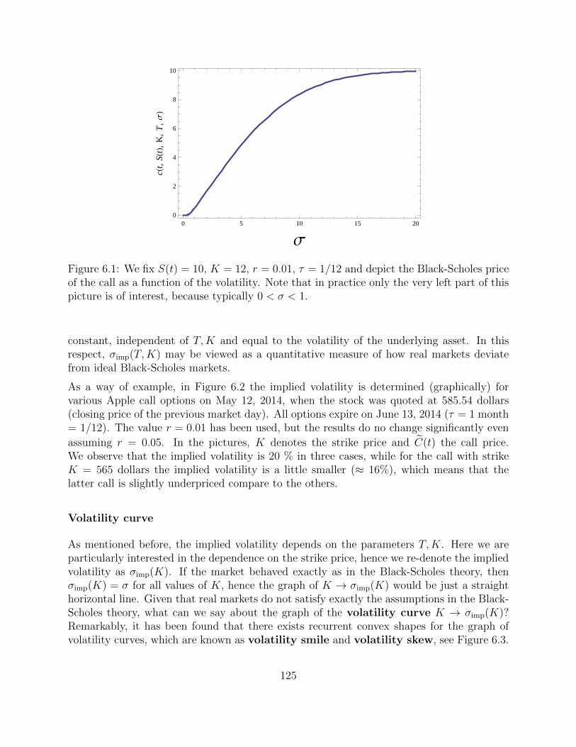
0 5 10 15 200

2

4

6

8

10

Σ

cHt,

SHtL

,K

,T

,Σ

L

Figure 6.1: We fix S(t) = 10, K = 12, r = 0.01, τ = 1/12 and depict the Black-Scholes priceof the call as a function of the volatility. Note that in practice only the very left part of thispicture is of interest, because typically 0 < σ < 1.

constant, independent of T,K and equal to the volatility of the underlying asset. In thisrespect, σimp(T,K) may be viewed as a quantitative measure of how real markets deviatefrom ideal Black-Scholes markets.

As a way of example, in Figure 6.2 the implied volatility is determined (graphically) forvarious Apple call options on May 12, 2014, when the stock was quoted at 585.54 dollars(closing price of the previous market day). All options expire on June 13, 2014 (τ = 1 month= 1/12). The value r = 0.01 has been used, but the results do no change significantly even

assuming r = 0.05. In the pictures, K denotes the strike price and C(t) the call price.We observe that the implied volatility is 20 % in three cases, while for the call with strikeK = 565 dollars the implied volatility is a little smaller (≈ 16%), which means that thelatter call is slightly underpriced compare to the others.

Volatility curve

As mentioned before, the implied volatility depends on the parameters T,K. Here we areparticularly interested in the dependence on the strike price, hence we re-denote the impliedvolatility as σimp(K). If the market behaved exactly as in the Black-Scholes theory, thenσimp(K) = σ for all values of K, hence the graph of K → σimp(K) would be just a straighthorizontal line. Given that real markets do not satisfy exactly the assumptions in the Black-Scholes theory, what can we say about the graph of the volatility curve K → σimp(K)?Remarkably, it has been found that there exists recurrent convex shapes for the graph ofvolatility curves, which are known as volatility smile and volatility skew, see Figure 6.3.

125

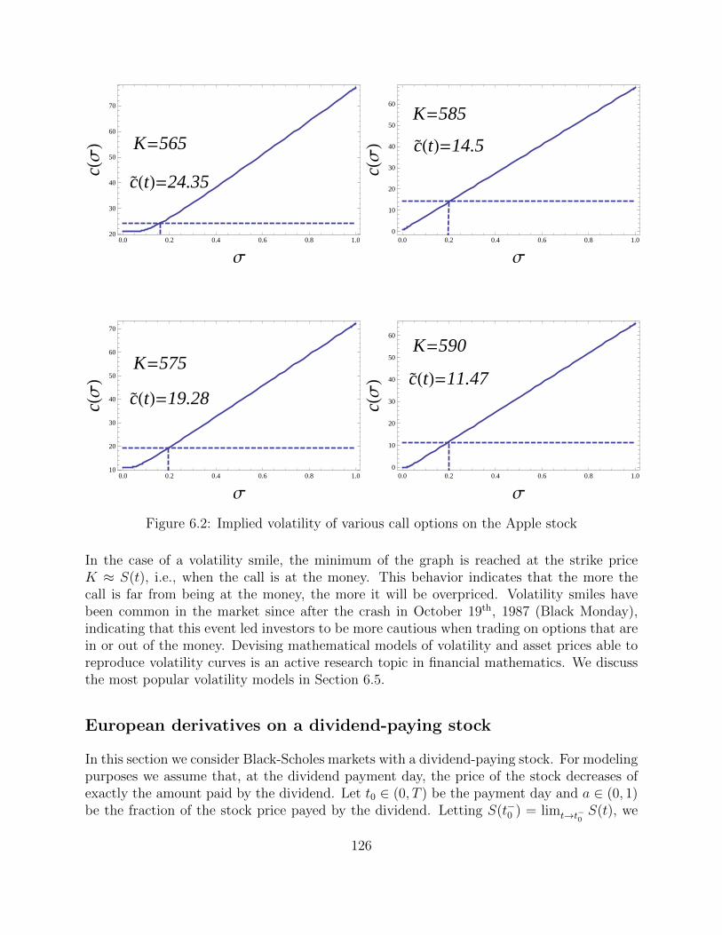
0.0 0.2 0.4 0.6 0.8 1.020

30

40

50

60

70

Σ

cHΣ

L K=565

cHtL=24.35

0.0 0.2 0.4 0.6 0.8 1.010

20

30

40

50

60

70

Σ

cHΣ

L

K=575

cHtL=19.28

0.0 0.2 0.4 0.6 0.8 1.00

10

20

30

40

50

60

Σ

cHΣ

L

K=585

cHtL=14.5

0.0 0.2 0.4 0.6 0.8 1.00

10

20

30

40

50

60

Σ

cHΣ

LK=590

cHtL=11.47

Figure 6.2: Implied volatility of various call options on the Apple stock

In the case of a volatility smile, the minimum of the graph is reached at the strike priceK ≈ S(t), i.e., when the call is at the money. This behavior indicates that the more thecall is far from being at the money, the more it will be overpriced. Volatility smiles havebeen common in the market since after the crash in October 19th, 1987 (Black Monday),indicating that this event led investors to be more cautious when trading on options that arein or out of the money. Devising mathematical models of volatility and asset prices able toreproduce volatility curves is an active research topic in financial mathematics. We discussthe most popular volatility models in Section 6.5.

European derivatives on a dividend-paying stock

In this section we consider Black-Scholes markets with a dividend-paying stock. For modelingpurposes we assume that, at the dividend payment day, the price of the stock decreases ofexactly the amount paid by the dividend. Let t0 ∈ (0, T ) be the payment day and a ∈ (0, 1)be the fraction of the stock price payed by the dividend. Letting S(t−0 ) = limt→t−0

S(t), we

126

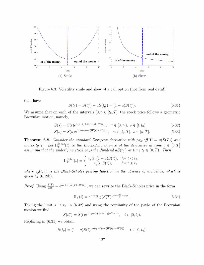
out of the moneyin of the money

0 2 4 6 8 1040

50

60

70

80

90

100

Strike

Implied

Vola

tility

(a) Smile

out of the money

in of the money

0 2 4 6 8 100

20

40

60

80

100

Strike

Implied

Vola

tility

(b) Skew

Figure 6.3: Volatility smile and skew of a call option (not from real data!)

then haveS(t0) = S(t−0 )− aS(t−0 ) = (1− a)S(t−0 ). (6.31)

We assume that on each of the intervals [0, t0), [t0, T ], the stock price follows a geometricBrownian motion, namely,

S(s) = S(t)eα(s−t)+σ(W (s)−W (t)), t ∈ [0, t0), s ∈ [t, t0) (6.32)

S(s) = S(u)eα(s−u)+σ(W (s)−W (u)), u ∈ [t0, T ], s ∈ [u, T ]. (6.33)

Theorem 6.8. Consider the standard European derivative with pay-off Y = g(S(T )) and

maturity T . Let Π(a,t0)Y (t) be the Black-Scholes price of the derivative at time t ∈ [0, T ]

assuming that the underlying stock pays the dividend aS(t−0 ) at time t0 ∈ (0, T ). Then

Π(a,t0)Y (t) =

vg(t, (1− a)S(t)), for t < t0,

vg(t, S(t)), for t ≥ t0,

where vg(t, x) is the Black-Scholes pricing function in the absence of dividends, which isgiven by (6.19b).

Proof. Using S(T )S(t)

= eατ+σ(W (T )−W (t)), we can rewrite the Black-Scholes price in the form

ΠY (t) = e−rτE[g(S(T )e(r−σ2

2−α)τ ]. (6.34)

Taking the limit s → t−0 in (6.32) and using the continuity of the paths of the Brownianmotion we find

S(t−0 ) = S(t)eα(t0−t)+σ(W (t0)−W (t)), t ∈ [0, t0).

Replacing in (6.31) we obtain

S(t0) = (1− a)S(t)eα(t0−t)+σ(W (t0)−W (t)), t ∈ [0, t0).

127

Hence, letting (s, u) = (T, t0) and (s, u) = (T, t) into (6.33), we find

S(T ) =

(1− a)S(t)eατ+σ(W (T )−W (t)) for t ∈ [0, t0),

S(t)eατ+σ(W (T )−W (t)) for t ∈ [t0, T ].(6.35)

By the definition of Black-Scholes price in the form (6.34) and denoting G = (W (T ) −W (t))/

√τ , we obtain

Π(a,t0)Y (t) = e−rτE[g((1− a)S(t)e(r−σ

2

2)τ+σ

√τG], for t ∈ [0, t0),

Π(a,t0)Y (t) = e−rτE[g(S(t)e(r−σ

2

2)τ+σ

√τG], for t ∈ [t0, T ].

As G ∈ N (0, 1), the result follows.

We conclude that for t ≥ t0, i.e., after the dividend has been paid, the Black-Scholes pricefunction of the derivative is again given by (6.19b), while for t < t0 it is obtained by replacingx with (1− a)x in (6.19b). To see the effect of this change, suppose that the derivative is acall option; let C(t, x) be the Black-Scholes price function in the absence of dividends andCa(t, x) be the price function in the case that a dividend is paid at time t0. Then, accordingto Theorem 6.8,

Ca(t, x) =

C(t, (1− a)x), for t < t0,

C(t, x), for t ≥ t0.

Since ∂xC > 0 (see Theorem 6.7), it follows that Ca(t, x) < C(t, x), for t < t0, that is to say,the payment of a dividend makes the call option on the stock less valuable (i.e., cheaper)than in the absence of dividends until the dividend is paid.

Exercise 6.14 (?). Give an intuitive explanation for the property just proved for call optionson a dividend paying stock.

Exercise 6.15 (Sol. 37). A standard European derivative pays the amount Y = (S(T ) −S(0))+ at time of maturity T . Find the Black-Scholes price ΠY (0) of this derivative at timet = 0 assuming that the underlying stock pays the dividend (1− e−rT )S(T

2−) at time t = T

2.

Compute the probability of positive return for a constant portfolio which is short 1 share ofthe derivative and short S(0)e−rT shares of the risk-free asset.

Exercise 6.16. Derive the Black-Scholes price of the derivative with pay-off Y = g(S(T )),assuming that the underlying pays a dividend at each time t1 < t2 < · · · < tM ∈ [0, T ].Denote by ai the dividend paid at time ti, i = 1, . . . ,M .

6.4 The Asian option

The Asian call option with strike K > 0 and maturity T > 0 is the non-standard Europeanstyle derivative with pay-off

YAC =

(1

T

∫ T

0

S(t) dt−K)

+

,

128

while for the Asian put the pay-off is

YAP =

(K − 1

T

∫ T

0

S(t) dt

)+

.

We study the Asian option in a Black-Scholes market, i.e., assuming that the market pa-rameters are deterministic constants. The risk-neutral price at time t ≤ T of the Asian callis therefore given by

ΠAC(t) = e−r(T−t)E[(Q(T )/T −K)+|FW (t)],

where

Q(t) =

∫ t

0

S(τ) dτ, S(τ) = S(0)e(r−σ2

2)τ+σW (τ).

Exercise 6.17 (Sol. 38). Prove the following put-call parity identity for Asian options:

ΠAC(t)− ΠAP(t) =Q(t)

Te−r(T−t) +

S(t)

rT(1− e−r(T−t))−Ke−r(T−t). (6.36)

To price the Asian option, we observe that the stochastic processes Q(t)t∈[0,T ], S(t)t∈[0,T ]

satisfy the system of SDE’s

dQ(t) = S(t) dt, dS(t) = rS(t) dt+ σS(t) dW (t).

By the Markov property of SDE’s it follows that the risk-neutral price of the Asian callsatisfies

ΠAC(t) = c(t, S(t), Q(t)). (6.37)

for some measurable function c.

Theorem 6.9. Let c : [0, T ]× (0,∞)2 → (0,∞) be the strong solution to the terminal valueproblem

∂tc+ rx∂xc+ x∂yc+σ2

2x2∂2

xc = rc, t ∈ (0, T ), x, y > 0 (6.38a)

c(T, x, y) = (y/T −K)+, x, y > 0. (6.38b)

Then (6.37) holds. Moreover the number of shares of the stock in the self-financing hedgingportfolio is given by hS(t) = ∂xc(t, S(t), Q(t)).

Proof. We have

d(e−rtc(t, S(t), Q(t)) = e−rt[∂tc+ rx∂xc+ x∂yc+σ2

2x2∂2

xc− rc](t, S(t), Q(t)) dt

+ e−rt∂xc(t, S(t))σS(t)dW (t).

129

As c satisfies (6.38), then

d(e−rtc(t, S(t), Q(t)) = e−rt∂xc(t, S(t), Q(t))σS(t)dW (t). (6.39)

It follows that the process e−rtc(t, S(t), Q(t))t∈[0,T ] is a P-martingale relative to FW (t)t∈[0,T ].In particular

e−rT E[c(T, S(T ), Q(T ))|FW (t)] = e−rtc(t, S(t), Q(t)), T ≥ t.

Using c(T, S(T ), Q(T )) = (Q(T )/T −K)+ proves (6.37). Moreover by (6.39) the discountedvalue of the Asian call satisfies

Π∗AC(t) = ΠAC(0) +

∫ t

0

e−rτ∂xc(τ, S(τ), Q(τ))σS(t) dW (τ),

hence by Theorem 6.2 the number of shares of the stock in the hedging portfolio is hS(t) =∂xc(t, S(t), Q(t)).

Remark 6.6. It can be shown that, as stated in the theorem, the problem (6.38) admitsa unique strong solution, although the proof requires a highly non-trivial generalization ofthe results presented in Chapter 5. In fact, while at any time t ∈ [0, T ] the solution is afunction of the two variables x, y, the diffusion operator (i.e., the second-order differentialoperator) acts only on the x variable. This type of PDE’s are called hypoelliptic and havebeen studied systematically by the Swedish mathematician Hormander (see [15]).

Exercise 6.18. Use Theorem 6.9 to give an alternative proof of the put-call parity (6.36)for Asian options.

A simple closed formula solution for the problem (6.38) is not available, hence one needsto rely on numerical methods to price Asian options. We describe below the Monte Carlomethod, which, due to its simplicity and despite not being very accurate, is very popularamong practitioners. A more robust and precise method is the finite difference methoddescribed in Chapter 5. To apply this method one needs to specify the boundary conditionsfor (6.38) at infinity and for x = 0, y > 0, y = 0, x > 0. Concerning the boundarycondition at x = 0, let c(t, y) = c(t, 0, y). Letting x = 0 in (6.38) we obtain that c satisfies∂tc = rc and c(T, y) = (y/T −K)+, from which we derive the boundary condition

c(t, 0, y) = e−r(T−t)( yT−K

)+. (6.40)

As to the boundary condition when y → ∞, we first observe that the Asian put becomesclearly worthless if Q(t) reaches arbitrarily large values. Hence the put-call parity (6.36)leads us to impose

c(t, x, y) ∼ y

Te−r(T−t), as y →∞, for all x > 0 (6.41)

The boundary conditions at y = 0 and x→∞ are not so obvious. The next theorem showsthat one can avoid giving these boundary conditions by a suitable variable transformation.

130

Theorem 6.10. Let u : [0,∞)× R→ [0,∞) be the strong solution to the problem

∂tu+σ2

2(γ(t)− z)2∂2

zu = 0, t ∈ (0, T ), z ∈ R (6.42a)

u(T, z) = (z)+, limz→−∞

u(t, z) = 0, limz→∞

(u(t, z)− z) = 0, t ∈ [0, T ), (6.42b)

where γ(t) = 1−e−r(T−t)rT

. Then the function

c(t, x, y) = xu

(t,

1

rT(1− e−r(T−t)) +

e−r(T−t)

x

( yT−K

))(6.43)

solves (6.38) as well as (6.40)-(6.41)

Proof. Proving that c solves the PDE in (6.38) is a straightforward calculation which isleft as an exercise. We now show that u satisfies the stated boundary conditions. First weobserve that c(T, x, y) = xu(T, x−1(y/T −K)) = x[x−1(y/T −K)]+ = (y/T −K)+, thus cverifies the terminal condition in (6.38). Now, for all x given, y → ∞ is equivalent to thesecond argument in the function (6.43) going to infinity, hence u ∼ z as z →∞ implies that,as y →∞,

c ∼ xz =x

rT(1− e−r(T−t)) + e−r(T−t)(y/T −K) ∼ e−r(T−t)y/T,

which proves (6.41). Similarly, the second argument in the function (6.43) tends to −∞if and only if x → 0+ and y/T − K < 0. Hence u → 0 as z → −∞ implies (6.40) fory/T −K < 0. When y > 0 is given such that y/T > K, we have that x → 0 is equivalentto the second argument in the function (6.43) diverging to ∞. Hence using u ∼ z as z →∞as before we have

c ∼ xz =x

rT(1− e−r(T−t)) + e−r(T−t)(y/T −K) ∼ e−r(T−t)(y/T −K), as x→ 0+,

which is (6.40) for y/T > K. Finally for y/T = K we have c(t, x, y) = xu(t, (1 −e−r(T−t))/rT )→ 0 as x→ 0+. This concludes the proof of the theorem.

Exercise 6.19. Prove that the function (6.43) solves the PDE in (6.38).

A project to analyze the Asian option by solving numerically the problem (6.42) is proposedin Appendix A at the end of the present chapter.

Exercise 6.20 (Sol. 39). Assume that the price S(t) of a stock follows a geometric Brownianmotion with instantaneous volatility σ > 0 and that the risk-free interest rate r is a positiveconstant. The Asian call with geometric average is the European style derivative with pay-off

Y =

(exp

( 1

T

∫ T

0

logS(t) dt)−K

)+

,

where T > 0 and K > 0 are respectively the maturity and strike of the call. Derive anexact formula for the Black-Scholes price of this option at time t = 0 and the correspondingput-call parity .

131

Monte Carlo analysis of the Asian option

A very popular method to compute numerically the price of non-standard derivatives is theMonte Carlo method. In this final section we describe briefly how the method works forAsian options and then leave the generalization to other derivatives as an exercise.

The Monte Carlo method

The Monte Carlo method is, in its simplest form, a numerical method to compute theexpectation of a random variable. Its mathematical validation is based on the Law ofLarge Numbers, which states the following: Suppose Xii≥1 is a sequence of i.i.d. randomvariables with expectation E[Xi] = µ. Then the sample average of the first n components ofthe sequence, i.e.,

Xn =1

n(X1 +X2 + · · ·+Xn),

converges (in probability) to µ.

The law of large numbers can be used to justify the fact that if we are given a large numberof independent trials X1, . . . , Xn of the random variable X, then

E[X] ≈ 1

n(X1 +X2 + · · ·+Xn).

To measure how reliable is the approximation of E[X] given by the sample average, considerthe standard deviation of the trials X1, . . . , Xn:

s =

√√√√ 1

n

n∑i=1

(Xn −Xi)2.

If we interpret X1, . . . , Xn as the first n components of a sequence Xii≥1 of i.i.d. randomvariables with E[Xi] = µ, then a simple application of the Central Limit Theorem provesthat the random variable

µ−Xn

s/√n

converges in distribution to a standard normal random variable. We use this result to showthat the true value µ of E[X] has about 95% probability to be in the interval

[Xn − 1.96s√n,Xn − 1.96

s√n

].

Indeed, for n large,

P(−1.96 ≤ µ−Xn

s/√n≤ 1.96

)≈∫ 1.96

−1.96

e−x2/2 dx√

2π≈ 0.95.

132

Application to options pricing theory

Consider now the European derivative with pay-off Y at maturity T . We approximate theprice at time t = 0 by

ΠY (0) = e−rT E[Y ] ≈ e−rTY1 + · · ·+ Yn

n(6.44)

where Y1, . . . , Yn is a large number of pay-off trials. As the pay-off depends on the path ofthe stock price, the trials Y1, . . . , Yn can be created by first generating a sample of paths forthe stock price. Letting 0 = t0 < t1 < · · · < tN = T be a partition of the interval [0, T ] withsize ti − ti−1 = h, we may construct a sample of n paths of the geometric Brownian motionon the given partition with the following simple Matlab function:

function Path=StockPath(s,sigma,r,T,N,n)

h=T/N;

W=randn(n,N);

q=ones(n,N);

Path=s*exp((r-sigma^2/2)*h.*cumsum(q’)+sigma*sqrt(h)*cumsum(W’));

Path=[s*ones(1,n);Path];

Note carefully that the stock price is modeled as a geometric Brownian motion with meanof log return α = r − σ2/2, which means that we are in the risk-neutral world. This is ofcourse correct, since the expectation in (6.44) that we want to compute is in the risk-neutralprobability measure.

In the case of the Asian call option with strike K and maturity T the pay-off is given by

Y =

(1

T

∫ T

0

S(t) dt−K)

+

≈(

1

N

N∑i=1

S(ti)−K)

+

.

The following function computes the approximate price of the Asian option using the MonteCarlo method:

function [price, conf95]=MonteCarlo AC(s,sigma,r,K,T,N,n)

tic

stockPath=StockPath(s,sigma,r,T,N,n);

payOff=max(0,mean(stockPath)-K);

price=exp(-r*T)*mean(payOff);

conf95=1.96*std(payOff)/sqrt(n);

toc

The function also return the 95% confidence interval of the result. For example, by runningthe command

[price, conf95]=MonteCarlo AC(100,0.5,0.05,100,1/2,100,1000000)

we get price=8.5799, conf95=0.0283, which means that the Black-Scholes price of the Asianoption with the given parameters has 95% probability to be in the interval 8.5799± 0.0283.

133

The calculation took about 4 seconds. Note that the 95% confidence is 0.0565/8.5799∗100 ≈0.66% of the price. The Monte Carlo method can be improved to achieve the same level ofaccuracy (or even better) with a much lower number of paths (and thus much quicker) thanin our example. See [18].

Exercise 6.21 (Matlab). Study numerically how the price of the Asian call and the con-fidence interval depend on the parameters of the option. Verify numerically the put-callparity (6.36) at time t = 0.

Exercise 6.22 (Matlab). One reason why investors prefer the Asian call to the standardcall is that the former is cheaper and less sensitive to volatility. Show numerically that thisis the case and give an intuitive explanation thereof.

Exercise 6.23 (Matlab). Look for the definition of Barrier options and Lookback options.Write a Matlab code that computes the price of these derivatives using the Monte Carlomethod. Study numerically the dependence of the price on the market parameters.

6.5 Local and Stochastic volatility models

In this and the next section we present a method to compute the risk-neutral price ofEuropean derivatives when the market parameters are not deterministic functions. We firstassume in this section that the interest rate of the money market is constant, i.e., R(t) = r,which is quite reasonable for derivatives with short maturity such as options; stochasticinterest rate models are important for pricing derivatives with long time of maturity, e.g.coupon bonds, which are discussed in Section 6.6. Assuming that the derivative is thestandard European derivative with pay-off function g and maturity T , the risk-neutral priceformula (6.1) becomes

ΠY (t) = e−rτ E[g(S(T ))|FW (t)], τ = T − t. (6.45)

Motivated by our earlier results on the Black-Scholes price, and Remark 6.3, we attempt tore-write the risk-neutral price formula in the form

ΠY (t) = vg(t, S(t)) for all t ∈ [0, T ], for all T > 0, (6.46)

for some function vg : D+T → (0,∞), which we call the pricing function of the derivative.

By (6.45), this is equivalent to

E[g(S(T ))|FW (t)] = erτvg(t, S(t)) (6.47)

i.e., to the property that S(t)t≥0 is a Markov process in the risk-neutral probability mea-

sure P, relative to the filtration FW (t)t≥0. At this point it remains to understand forwhich stochastic processes σ(t)t≥0 does the generalized geometric Brownian motion (6.4)satisfies this Markov property. We have seen in Section 5.1 that this holds in particular whenS(t)t≥0 satisfies a (system of) stochastic differential equation(s), see Section 5.1. Next wediscuss two examples which encompass most of the volatility models used in the applications:Local volatility models and Stochastic volatility models.

134

Local volatility models

A local volatility model is a special case of the generalized geometric Brownian motionin which the instantaneous volatility of the stock σ(t)t≥0 is assumed to be a deterministicfunction of the stock price S(t). Given a continuous function β : [0,∞) × [0,∞) → (0,∞),we then let

σ(t)S(t) = β(t, S(t)), (6.48)

into (6.4), so that the stock price process S(t)t≥0 satisfies the SDE

dS(t) = rS(t) dt+ β(t, S(t))dW (t), S(0) = S0 > 0. (6.49)

We assume that this SDE admits a unique global solution, which is true in particular underthe assumptions of Theorem 5.1. To this regard we observe that the drift term α(t, x) = rxin (6.49) satisfies both (5.3) and (5.4), hence these conditions restrict only the form of thefunction β(t, x). In the following we shall also assume that the solution S(t)t≥0 of (6.49)is non-negative a.s. for all t > 0. Note however that the stochastic process solution of (6.49)will in general hit zero with positive probability at any finite time. For example, lettingβ(t, x) =

√x, the stock price (6.49) is a CIR process (5.27) with b = 0 and so, according to

Theorem 5.6, S(t) = 0 with positive probability for all t > 0.

Theorem 6.11. Let g ∈ G and assume that the Kolmogorov PDE

∂tu+ rx∂xu+1

2β(t, x)2∂2

xu = 0 (t, x) ∈ D+T , (6.50)

associated to (6.49) admits a (necessarily unique) strong solution in the region D+T satisfying

u(T, x) = g(x). Let alsovg(t, x) = e−rτu(t, x).

Then we have the following.

(i) vg satisfies

∂tvg + rx∂xvg +1

2β(t, x)2∂2

xvg = rvg (t, x) ∈ D+T , (6.51)

and the terminal conditionvg(T, x) = g(x). (6.52)

(ii) The price of the European derivative with pay-off Y = g(S(T )) and maturity T > 0 isgiven by (6.46).

(iii) The portfolio given by

hS(t) = ∂xvg(t, S(t)), hB(t) = (ΠY (t)− hS(t)S(t))/B(t)

is a self-financing hedging portfolio.

135

Proof. (i) It is straightforward to verify that vg satisfies (6.51).

(ii) Let X(t) = vg(t, S(t)). By Ito’s formula we find

dX(t) = (∂tvg(t, S(t)) + rS(t)∂xvg(t, S(t)) +1

2β(t, S(t))2∂2

xvg(t, S(t)))dt

+ β(t, S(t))∂xvg(t, S(t))dW (t).

Hence

d(e−rtX(t)) = e−rt(∂tvg + rx∂xvg +1

2β(t, x)2∂2

xvg − rvg)(t, S(t))dt

+ e−rtβ(t, S(t))∂xvg(t, S(t))dW (t).

As vg(t, x) satisfies (6.51), the drift term in the right hand side of the previous equation iszero. Hence

e−rtvg(t, S(t)) = vg(t, S0) +

∫ t

0

e−ruβ(u, S(u))∂xvg(u, S(u))dW (u). (6.53)

It follows that3 the stochastic process e−rtvg(t, S(t))t≥0 is a P-martingale relative to FW (t)t≥0.Hence

E[e−rTvg(T, S(T ))|FW (t)] = e−rtvg(t, S(t)), for all 0 ≤ t ≤ T .

Using the boundary condition (6.52), we find

vg(t, S(t)) = e−rτ E[g(S(T ))|FW (t)],

which proves (6.46).

(iii) Replacing ΠY (t) = vg(t, S(t)) into (6.53), we find

Π∗Y (t) = ΠY (0) +

∫ t

0

e−ruβ(u, S(u))∂xvg(u, S(u))dW (u).

Hence the claim on the hedging portfolio follows by Theorem 6.2.

A closed formula for the solution of (6.50) is rarely available, hence to compute the price ofthe derivative one needs to rely on numerical methods, such as those discussed in Section 5.4.

Example: The CEV model

For the constant elasticity variance (CEV) model, we have β(t, S(t)) = σS(t)δ, whereσ > 0, δ > 0 are constants. The SDE for the stock price becomes

dS(t) = rS(t)dt+ σS(t)δdW (t), S(0) = S0 > 0. (6.54)

3Recall that we assume that Ito’s integrals are martingales!

136

For δ = 1 we recover the Black-Scholes model. For δ 6= 1, we can construct the solutionof (6.54) using a CIR process, as shown in the following exercise.

Exercise 6.24. Given σ, r and δ 6= 1, define

a = 2r(δ − 1), c = −2σ(δ − 1), b =σ2

2r(2δ − 1), θ = − 1

2(δ − 1).

Let X(t)t≥0 be the CIR process

dX(t) = a(b−X(t)) dt+ c√X(t)dW (t), X(0) = x > 0.

Show that S(t) = X(t)θ solves (6.54) with S0 = xθ.

It follows by Exercise 6.24, and by Feller’s condition ab ≥ c2/2 for the positivity of the CIRprocess, that the solution of (6.54) remains strictly positive a.s. if δ ≥ 1, while for 0 < δ < 1,the stock price hits zero in finite time with positive probability.

The Kolmogorov PDE (6.50) associated to the CEV model is

∂tu+ rx∂xu+σ2

2x2δ∂2

xu = 0, (t, x) ∈ D+T .

Given a terminal value g at time T as in Theorem 6.11, the previous equation admits aunique solution. However a fundamental solution, in the sense of Theorem 5.5, exists onlyfor δ > 1, as otherwise the stochastic process S(t)t≥0 hits zero at any finite time withpositive probability and therefore the density of the random variable S(t) has a discretepart. The precise form of the (generalized) density fS(t)(x) in the CEV model is known forall values of δ and are given for instance in [20]. An exact formula for call options can befound in [24]. A project that aims to analyze the CEV model by the finite difference methodis proposed in Appendix B at the end of the present chapter.

Stochastic volatility models

For local volatility models, the stock price and the instantaneous volatility are both stochasticprocesses. However there is only one source of randomness which drives both these processes,namely a single Brownian motion W (t)t≥0. The next level of generalization consists inassuming that the stock price and the volatility are driven by two different sources of ran-domness.

Definition 6.4. Let W1(t)t≥0, W2(t)t≥0 be two independent Brownian motions andFW (t)t≥0 be their own generated filtration. Let ρ ∈ [−1, 1] be a deterministic constantand µ, η, β : [0,∞)3 → R be continuous functions. A stochastic volatility model is a pairof (non-negative) stochastic diffusion processes S(t)t≥0, v(t)t≥0 satisfying the followingsystem of SDE’s:

dS(t) = µ(t, S(t), v(t))S(t) dt+√v(t)S(t) dW1(t), (6.55)

dv(t) = η(t, S(t), v(t)) dt+ β(t, S(t), v(t))√v(t)(ρ dW1(t) +

√1− ρ2 dW2(t)). (6.56)

137

We see from (6.55) that v(t)t≥0 is the instantaneous variance of the stock price S(t)t≥0.Moreover the process W (ρ)(t)t≥0 given by

W (ρ)(t) = ρW1(t) +√

1− ρ2W2(t)

is a Brownian motion satisfying

dW1(t)dW (ρ)(t) = ρ dt;

in particular the two Brownian motions W1(t)t≥0, W (ρ)t≥0 are not independent, as theircross variation is not zero; in fact, by Exercise 4.4, ρ is the correlation of the two Brownianmotions. Hence in a stochastic volatility model the stock price and the volatility are bothstochastic processes driven by two correlated Brownian motions. We assume that S(t)t≥0

is non-negative and v(t)t≥0 is positive a.s. for all times, although we refrain from discussingunder which general conditions this is verified (we will present an example below).

Our next purpose is to introduce a risk-neutral probability measure such that the discountedprice of the stock is a martingale. As we have two Brownian motions in this model, we shallapply the two-dimensional Girsanov Theorem 4.11 to construct such a probability measure.Precisely, let r > 0 be the constant interest rate of the money market and γ : [0,∞)3 → Rbe a continuous function We define

θ1(t) =µ(t, S(t), v(t))− r√

v(t), θ2(t) = γ(t, S(t), v(t)), θ(t) = (θ1(t), θ2(t)).

Given T > 0, we introduce the new probability measure P(γ) equivalent to P by P(γ)(A) =E[Z(T )IA], for all A ∈ F , where

Z(t) = exp

(−∫ t

0

θ1(s) dW1(s)−∫ t

0

θ2(s) dW2(s)− 1

2

∫ t

0

‖θ(s)‖2 ds

).

Then by Theorem 4.11, the stochastic processes

W1(t) = W1(t) +

∫ t

0

θ1(s) ds, W(γ)2 (t) = W2(t) +

∫ t

0

γ(s) ds

are two P(γ)-independent Brownian motions. Moreover (6.55)-(6.56) can be rewritten as

dS(t) = rS(t)dt+√v(t)S(t)dW1(t), (6.57a)

dv(t) = [η(t, S(t), v(t))−√v(t)ψ(t, S(t), v(t))β(t, S(t), v(t))]dt

+ β(t, S(t), v(t))√v(t)dW (ρ,γ), (6.57b)

where ψ(t, S(t), v(t))t≥0 is the FW (t)t≥0-adapted stochastic process given by

ψ(t, S(t), v(t)) =µ(t, S(t), v(t))− r√

v(t)ρ+ γ(t, S(t), v(t))

√1− ρ2 (6.58)

138

and whereW (ρ,γ)(t) = ρW1(t) +

√1− ρ2W

(γ)2 (t).

Note that the P(γ)-Brownian motions W1(t)t≥0, W (ρ,γ)(t)t≥0 satisfy

dW1(t)dW (ρ,γ)(t) = ρdt, for ρ ∈ [−1, 1]. (6.59)

It follows immediately that the discounted price e−rtS(t)t≥0 is a P(γ)-martingale relative

to the filtration FW (t)t≥0. Hence all probability measures P(γ) are equivalent risk-neutralprobability measures.

Remark 6.7 (Incomplete markets). As the risk-neutral probability measure is not uniquelydefined, the market under discussion is said to be incomplete. Within incomplete marketsthere is no unique value for the price of derivatives (it depends on which specific risk-neutralprobability measure is used to price the derivative). The stochastic process ψ(t)t≥0 iscalled the market price of volatility risk and reduces to (6.3) for γ ≡ 0 (or ρ = 1).

Consider now the standard European derivative with pay-off Y = g(S(T )) at time of maturityT . For stochastic volatility models it is reasonable to assume that the risk-neutral price ΠY (t)of the derivative is a local function of the stock price and of the instantaneous variance, i.e.,we make the following ansatz which generalizes (6.46):

ΠY (t) = e−r(T−t)E[g(S(T ))|FW (t)] = vg(t, S(t), v(t)) (6.60)

for all t ∈ [0, T ], for all T > 0 and for some measurable pricing vg. Of course, as in the caseof local volatility models, (6.60) is motivated by the Markov property of solutions to systemsof SDE’s. In fact, it is useful to consider a more general European derivative with pay-off Ygiven by

Y = h(S(T ), v(T )),

for some function h : [0,∞)2 → R, i.e., the pay-off of the derivative depends on the stockvalue and on the instantaneous variance of the stock at the time of maturity. We have thefollowing analogue of Theorem 6.11.

Theorem 6.12. Assume that the functions η(t, x, y), β(t, x, y), ψ(t, x, y) in (6.57) are suchthat the PDE

∂tu+ rx∂xu+ A∂yu+1

2yx2∂2

xu+1

2β2y∂2

yu+ ρβxy∂2xyu = 0, (6.61a)

A = η −√yβψ, (t, x, y) ∈ (0, T )× (0,∞)2 (6.61b)

admits a unique strong solution u satisfying u(T, x, y) = h(x, y). Then the risk-neutral priceof the derivative with pay-off Y = h(S(T ), v(T )) and maturity T is given by

ΠY (t) = fh(t, S(t), v(t))

where the pricing function fh is given by fh(t, x, y) = e−rτu(t, x, y), τ = T − t.

139

Exercise 6.25. Prove the theorem. Hint: use Ito’s formula in two dimensions, see Theo-rem 4.8, and the argument in the proof of Theorem 6.11.

As for the local volatility models, a closed formula solution of (6.61) is rarely available andthe use numerical methods to price the derivative becomes essential.

Heston model

A popular stochastic volatility model is the Heston model, which is obtained by the followingsubstitutions in (6.55)-(6.56):

µ(t, S(t), v(t)) = µ0, β(t, x, y) = c, η(t, x, y) = a(b− y),

where µ0, a, b, c are constant. Hence the stock price and the volatility dynamics in the Hestonmodel are given by the following stochastic differential equations:

dS(t) = µ0S(t) dt+√v(t)S(t)dW1(t), (6.62a)

dv(t) = a(b− v(t))dt+ c√v(t)dW (ρ)(t). (6.62b)

Note in particular that the variance in the Heston model is a CIR process in the physicalprobability P, see (5.27). The condition 2ab ≥ c2 ensures that v(t) is strictly positive almostsurely. To pass to the risk neutral world we need to fix a risk-neutral probability measure,that is, we need to fix the market price of volatility risk function ψ in (6.58). In the Hestonmodel it is assumed that

ψ(t, x, y) = λ√y, (6.63)

for some constant λ ∈ R, which leads to the following form of the pricing PDE (6.61):

∂tu+ rx∂xu+ (k −my)∂yu+1

2yx2∂2

xu+c2

2y∂2

yu+ ρcxy∂2xyu = 0, (6.64)

where the constant k,m are given by k = ab, m = (a + cλ). Note that the choice (6.63)implies that the variance of the stock remains a CIR process in the risk-neutral probabilitymeasure.

The general solution of (6.64) with terminal datum u(T, x, y) = h(x, y) is not known. How-ever in the case of a call option (i.e., h(x, y) = g(x) = (x−K)+) an explicit formula for theFourier transform of the solution is available, see [14]. With this formula at hand one cancompute the price of call options by very efficient numerical methods, which is one of themain reasons for the popularity of the Heston model.

140

Variance swaps

Variance swaps are financial derivatives4 on the realized annual variance of an asset (orindex). We first describe how the realized annual variance is computed from the historicaldata of the asset price. Let T > 0 be measured in days and consider the partition

0 = t0 < t1 < · · · < tn = T, tj+1 − tj = h > 0,

of the interval [0, T ]. Assume for instance that the asset is a stock and let S(tj) = Sj be thestock price at time tj. Here S1, . . . Sn are historical data for the stock price and not randomvariables (i.e., the interval [0, T ] lies in the past of the present time). The realized annualvariance of the stock in the interval [0, T ] along this partition is defined as

σ21year(n, T ) =

κ

T

n−1∑j=0

(log

Sj+1

Sj− 1

nlog

S(T )

S(0)

)2

, (6.65)

where κ is the number of trading days in one year (typically, κ = 252). Using T = nh wesee that, up to a normalization factor, (6.65) coincides with the sample variance of the log-returns of the stock in the intervals [tj, tj+1], j = 0, . . . , n− 1. A variance swap stipulatedat time t = 0, with maturity T and strike variance K is a contract between two partieswhich, at the expiration date, entails the exchange of cash given by N(σ2

1year−K), where N(called variance notional) is a conversion factor from units of variance to units of currency.In particular, the holder of the long position on the swap is the party who receives the cashin the case that the realized annual variance at the expiration date is larger than the strikevariance. Variance swaps are traded over the counter and they are used by investors toprotect their exposure to the volatility of the asset. For instance, suppose that an investorhas a position on an asset which is profitable if the volatility of the stock price increases (e.g.,the investor owns call options on the stock). Then it is clearly important for the investorto secure such position against a possible decrease of the volatility. To this purpose theinvestor opens a short position on a variance swap with another investor who is exposed tothe opposite risk.

Let us now discuss variance swaps from a mathematical modeling point of view. We assumethat the stock price follows the generalized geometric Brownian motion

S(t) = S(0) exp

(∫ t

0

α(s)ds+

∫ t

0

σ(s)dW (s)

).

Next we show that, as n→∞, the realized annual variance in the future time interval [0, T ]converges in L2 to the random variable

QT =κ

T[logS, logS](T ) =

κ

T

∫ T

0

σ2(t) dt.

4More precisely, forward contracts, see Section 6.7.

141

To see this we first rewrite the definition of realized annual variance as

σ21year(n, T ) =

κ

T

n−1∑j=0

(log

Sj+1

Sj

)2

− κ

nT

(log

S(T )

S(0)

)2

. (6.66)

Hence

limn→∞

σ21year(n, T ) = lim

n→∞

κ

T

n−1∑j=0

(log

Sj+1

Sj

)2

in L2.

Moreover, by the definition of quadratic variation, it follows that

E

( κT

n−1∑j=0

(log

Sj+1

Sj

)2

−QT

)2→ 0, as n→∞.

A variance swap can thus be defined as the (non-standard) European derivative with pay-offY = QT −K. Assuming that the interest rate of the money market is the constant r ∈ R,the risk-neutral value of a variance swap is given by

ΠY (t) = e−rτ E[QT −K|FW (t)]. (6.67)

In particular, at time t = 0, i.e., when the contract is stipulated, we have

ΠY (0) = e−rT E[QT −K], (6.68)

where we used that FW (0) is a trivial σ-algebra, and therefore the conditional expectationwith respect to FW (0) is a pure expectation. As none of the two parties in a variance swaphas a privileged position on the contract, there is no premium associated to variance swaps,that is to say, the fair value of a variance swap is zero5. The value K∗ of the variance strikewhich makes the risk-neutral price of a variance swap equal to zero at time t = 0, i.e.,ΠY (0) = 0, is called the fair variance strike. By (6.68) we find

K∗ =κ

T

∫ T

0

E[σ2(t)] dt. (6.69)

To computeK∗ explicitly, we need to fix a stochastic model for the variance process σ2(t)t≥0.Let us consider the Heston model

dσ2(t) = a(b− σ2(t))dt+ cσ(t)dW (t), (6.70)

where a, b, c are positive constants satisfying 2ab ≥ c2 and where W (t)t≥0 is a Brownianmotion in the risk-neutral probability measure. To compute the fair variance strike of theswap using the Heston model we use that

E[σ2(t)] = abt− a∫ t

0

E[σ2(s)] ds,

5This is a general property of forward contracts, see Section 6.7.

142

which implies ddtE[σ2(t)] = ab− aE[σ2(t)] and so

E[σ2(t)] = b+ (σ20 − b)e−at, σ2

0 = E[σ2(0)] = σ2(0). (6.71)

Replacing into (6.69) we obtain

K∗ = κ

[b+

σ20 − baT

(1− e−aT )

].

Exercise 6.26 (Sol. 40). Given σ0 > 0, let σ(t) = σ0

√S(t), which is an example of CEV

model. Compute the fair strike of the variance swap.

Exercise 6.27 (Sol. 41). Assume that the price S(t) of a stock follows a generalized geometricBrownian motion with instantaneous volatility σ(t)t≥0 given by the Heston model dσ2(t) =

a(b − σ2(t)) dt + cσ(t) dW (t), where W (t)t≥0 is a Brownian motion in the risk-neutralprobability measure and a, b, c are constants such that 2ab ≥ c2 > 0. The volatility calloption with strike K and maturity T is the financial derivative with pay-off

Y = N

√ κ

T

∫ T

0

σ2(t) dt−K

+

,

where κ is the number of trading days in one year and N is a dimensional constant that con-verts units of volatility into units of currency. Assuming that the interest rate of the moneymarket is constant, find the partial differential equation and the terminal value satisfied bythe pricing function of the volatility option.

6.6 Interest rate contracts

Zero-coupon bonds

A zero-coupon bond (ZCB) with face (or nominal) value K and maturity T > 0 is acontract that promises to pay to its owner the amount K at time T in the future. Zero-coupon bonds, and related contracts described below, are issued by national governmentsand private companies as a way to borrow money and fund their activities. In the followingwe assume that all ZCB’s are issued by one given institution, so that all bonds differ merelyby their face values and maturities. Moreover without loss of generality we assume from nowon that K = 1, as owning a ZCB with face value K is clearly equivalent to own K shares ofa ZCB with face value 1.

Once a debt is issued in the so-called primary market, it becomes a tradable asset in thesecondary bond market. It is therefore natural to model the value at time t of the ZCBmaturing at time T > t (and face value 1) as a random variable, which we denote by B(t, T ).

143

We assume throughout the discussion that the institution issuing the bond bears no risk ofdefault, i.e., B(t, T ) > 0, for all t ∈ [0, T ]. Clearly B(T, T ) = 1 and, under normal marketconditions, B(t, T ) < 1, for t < T , although exceptions are not rare6. A zero-couponbond market (ZCB market) is a market in which the objects of trading are ZCB’s withdifferent maturities. Our main goal is to introduce models for the prices of ZCB’s observedin the market. For modeling purposes we assume that zero-coupon bonds are available witha continuum range of maturities T ∈ [0, S], where S > 0 is sufficiently large so that allZCB’s in the market mature before the time S (e.g., S ≈ 50 years). Mathematically thismeans that we model the prices of ZCB’s in the market as a stochastic process dependingon 2 parameters, namely

B(t, T ), t ∈ [0, T ], T ∈ [0, S].All processes X(t, T ), t ∈ [0, T ], T ∈ [0, S] introduced in this section are assumed to havea.s. continuous paths in both variables t, T and to be adapted to the filtration FW (t)t≥0

generated by the given Brownian motion W (t)t≥0. This means that for all given T ∈ [0, S],the stochastic process X(t, T )t∈[0,T ] is adapted to FW (t)t≥0. By abuse of notation wecontinue to denote by C0[FW (t)] this class of processes.

Remark 6.8. The term “bond” is more specifically used for long term loans with maturityT > 1 year. Short term loans have different names (e.g., bills, repo, etc.) and they constitutethe component of the loan market called money market. A bond which has less than oneyear left to maturity is also considered a money market asset.

Forward and spot rate

The difference in value of zero-coupon bonds with different maturities is expressed throughthe implied forward rate of the bond. To define this concept, suppose first that at the presenttime t we open a portfolio that consists of −1 share of a zero-coupon bond with maturityT > t and B(t, T )/B(t, T + δ) shares of a zero-coupon bond expiring at time T + δ. Notethat the value of this portfolio is V (t) = 0. This investment entails that we pay 1 at time Tand receive B(t, T )/B(t, T + δ) at time T + δ. Hence our investment at time t is equivalentto an investment in the future time interval [T, T + δ] with (annualized) return given by

Fδ(t, T ) =1

δ(B(t, T )/B(t, T + δ)− 1) =

B(t, T )−B(t, T + δ)

δB(t, T + δ). (6.72)

The quantity Fδ(t, T ) is also called the simply compounded forward rate in the interval[T, T+δ] locked at time t (or forward LIBOR, as it is commonly applied to LIBOR interestrate contracts). The name is intended to emphasize that the return in the future interval[T, T + δ] is locked at the time t ≤ T , that is to say, we know today which interest rate hasto be charged to borrow in the future time interval [T, T + δ] (if a different rate were locked

6For instance, zero-coupon (and other) national bonds in Sweden with maturity shorter than 5 years yieldcurrently (2017) a negative return.

144

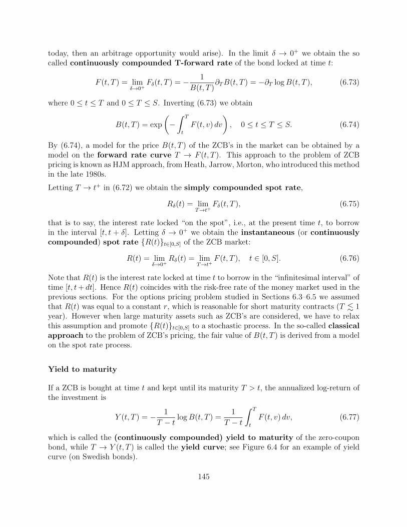
today, then an arbitrage opportunity would arise). In the limit δ → 0+ we obtain the socalled continuously compounded T-forward rate of the bond locked at time t:

F (t, T ) = limδ→0+

Fδ(t, T ) = − 1

B(t, T )∂TB(t, T ) = −∂T logB(t, T ), (6.73)

where 0 ≤ t ≤ T and 0 ≤ T ≤ S. Inverting (6.73) we obtain

B(t, T ) = exp

(−∫ T

t

F (t, v) dv

), 0 ≤ t ≤ T ≤ S. (6.74)

By (6.74), a model for the price B(t, T ) of the ZCB’s in the market can be obtained by amodel on the forward rate curve T → F (t, T ). This approach to the problem of ZCBpricing is known as HJM approach, from Heath, Jarrow, Morton, who introduced this methodin the late 1980s.

Letting T → t+ in (6.72) we obtain the simply compounded spot rate,

Rδ(t) = limT→t+

Fδ(t, T ), (6.75)

that is to say, the interest rate locked “on the spot”, i.e., at the present time t, to borrowin the interval [t, t + δ]. Letting δ → 0+ we obtain the instantaneous (or continuouslycompounded) spot rate R(t)t∈[0,S] of the ZCB market:

R(t) = limδ→0+

Rδ(t) = limT→t+

F (t, T ), t ∈ [0, S]. (6.76)

Note that R(t) is the interest rate locked at time t to borrow in the “infinitesimal interval” oftime [t, t+ dt]. Hence R(t) coincides with the risk-free rate of the money market used in theprevious sections. For the options pricing problem studied in Sections 6.3–6.5 we assumedthat R(t) was equal to a constant r, which is reasonable for short maturity contracts (T . 1year). However when large maturity assets such as ZCB’s are considered, we have to relaxthis assumption and promote R(t)t∈[0,S] to a stochastic process. In the so-called classicalapproach to the problem of ZCB’s pricing, the fair value of B(t, T ) is derived from a modelon the spot rate process.

Yield to maturity

If a ZCB is bought at time t and kept until its maturity T > t, the annualized log-return ofthe investment is

Y (t, T ) = − 1

T − t logB(t, T ) =1

T − t

∫ T

t

F (t, v) dv, (6.77)

which is called the (continuously compounded) yield to maturity of the zero-couponbond, while T → Y (t, T ) is called the yield curve; see Figure 6.4 for an example of yieldcurve (on Swedish bonds).

145

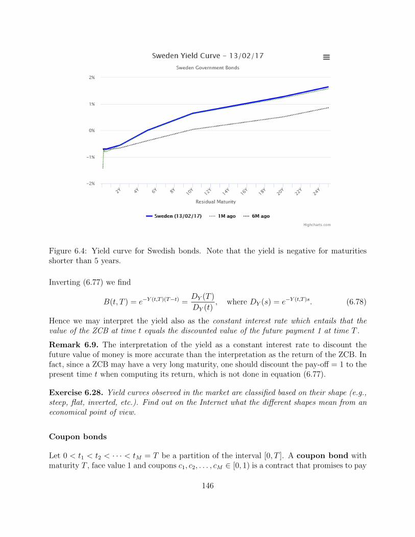
Figure 6.4: Yield curve for Swedish bonds. Note that the yield is negative for maturitiesshorter than 5 years.

Inverting (6.77) we find

B(t, T ) = e−Y (t,T )(T−t) =DY (T )

DY (t), where DY (s) = e−Y (t,T )s. (6.78)

Hence we may interpret the yield also as the constant interest rate which entails that thevalue of the ZCB at time t equals the discounted value of the future payment 1 at time T .

Remark 6.9. The interpretation of the yield as a constant interest rate to discount thefuture value of money is more accurate than the interpretation as the return of the ZCB. Infact, since a ZCB may have a very long maturity, one should discount the pay-off = 1 to thepresent time t when computing its return, which is not done in equation (6.77).

Exercise 6.28. Yield curves observed in the market are classified based on their shape (e.g.,steep, flat, inverted, etc.). Find out on the Internet what the different shapes mean from aneconomical point of view.

Coupon bonds

Let 0 < t1 < t2 < · · · < tM = T be a partition of the interval [0, T ]. A coupon bond withmaturity T , face value 1 and coupons c1, c2, . . . , cM ∈ [0, 1) is a contract that promises to pay

146

the amount ck at time tk and the amount 1+cM at maturity T = tM . Note that some ck maybe zero, which means that no coupon is actually paid at that time. We set c = (c1, . . . , cM)and denote by Bc(t, T ) the value at time t of the bond paying the coupons c1, . . . , cM andmaturing at time T . Now, let t ∈ [0, T ] and k(t) ∈ 1, . . . ,M be the smallest index suchthat tk(t) > t, that is to say, tk(t) is the first time after t at which a coupon is paid. Holdingthe coupon bond at time t is clearly equivalent to holding a portfolio containing ck(t) sharesof the ZCB expiring at time tk(t), ck(t)+1 shares of the ZCB expiring at time tk(t)+1, and soon, hence

Bc(t, T ) =M−1∑j=k(t)

cjB(t, tj) + (1 + cM)B(t, T ), (6.79)

the sum being zero when k(t) = M .

Remark 6.10. The value of the coupon bond at time t does not depend on the couponspaid at or before t. This of course makes sense, because purchasing a bond at time t doesnot give the buyer any right concerning previous coupon payments.

The yield to maturity of a coupon bond is the quantity Yc(t, T ) defined implicitly by theequation

Bc(t, T ) =M−1∑j=k(t)

cje−Yc(t,T )(tj−t) + (1 + cM)e−Yc(t,T )(T−t). (6.80)

It follows that the yield of the coupon bond is the constant interest rate used to discount thetotal future payments of the coupon bond.

Example. Consider a 3 year maturity coupon bond with face value 1 which pays 2% couponsemiannually. Suppose that the bond is listed with an yield of 1%. What is the value of thebond at time zero? The coupon dates are

(t1, t2, t3, t4, t5, t6) = (1/2, 1, 3/2, 2, 5/2, 3),

and c1 = c2 = · · · = c6 = 0.02. Hence

Bc(0, T ) = 0.02e−0.01∗ 12 + 0.02e−0.01∗1 + 0.02e−0.01∗ 3

2 + 0.02e−0.01∗2 + 0.02e−0.01∗ 52

+ (1 + 0.02)e−0.01∗3 = 1.08837.

Remark 6.11. As in the previous example, the coupons of a coupon bond are typically allequal, i.e., c1 = c2 = · · · = cM = c ∈ (0, 1).

In the example above, the yield was given and Bc(0, T ) was computed. However one is mostcommonly faced with the opposite problem, i.e., computing the yield of the coupon bond withgiven initial value Bc(0, T ). We can easily solve this problem numerically inverting (6.80).For instance, assume that the bond is issued at time t = 0 with maturity T = M years (M

147

integer) and that the coupons are paid annually, that is t1 = 1, t2 = 2, . . . , tM = M . Thenx = exp(−Yc(0, T )) solves p(x) = 0, where p is the M -order polynomial given by

p(x) = c1x+ c2x2 + · · ·+ (1 + cM)xM −Bc(0, T ). (6.81)

The roots of this polynomial can easily be computed numerically, e.g., with the commandroots[p] in matlab, see Exercise 6.29 below.

Exercise 6.29 (Matlab). Write a matlab function

yield(B, Coupon, FirstCoupDate, CoupFreq, T)

that computes the yield of a coupon bond. Here, B is the current (i.e., at time t = 0) priceof the coupon, Coupon ∈ [0, 1) is the (constant) coupon, FirstCoupDate is the first futuredate at which the coupon is paid, CoupFreq is the frequency of coupon payments and T isthe maturity of the coupon bond. Express all time in fraction of years, using 1 day = 1/252years. For example

yield(1.01, 0.02, 46/252, 1, 4)

computes the yield of a 2% coupon bond which today is valued 1.01, pays the first coupon in46 days and expires in 4 years.

Classical approach to ZCB pricing

In the so-called classical approach to the problem of pricing ZCB’s we interpret the ZCB asa derivative on the spot rate. Assume that a model for R(t)t∈[0,S] is given as a stochasticprocess in the space C0[FW (t)]. As the pay-off of the ZCB equals one, the risk-neutral priceof the ZCB is given by

B(t, T ) = E[D(t)−1D(T )|FW (t)] = E[

exp(−∫ T

t

R(s) ds)|FW (t)]

(6.82)

and by Theorem 6.2(i) (with Y = 1), the discounted price of the ZCB,B∗(t, T ) = D(t)B(t, T ),

is a P-martingale relative to FW (t)t≥0; in particular, self-financing portfolios invested inthe ZCB market are not arbitrage portfolios. Note however that the risk-neutral probabilitymeasure in (6.82) cannot be determined solely by the spot rate, and therefore models for theprocess R(t)t∈[0,S] must be given a priori in terms of a risk-neutral probability measure. Asthe real world is not risk-neutral, the foundation of the classical approach is questionable.There are two ways to get around this problem. One is the HJM approach described below;the other is by adding a risky asset (e.g. a stock) to the ZCB market, which would then beused to determine the risk-neutral probability measure. The last procedure is referred to as“completing the ZCB market” and will be discussed in Section 6.7.

As an application of the classical approach, assume that the spot rate is given by the Cox-Ingersoll-Ross (CIR) model,

dR(t) = a(b−R(t))dt+ c√R(t)dW (t), R(0) = R0 > 0, (6.83)

148

where W (t)t∈[0,T ] is a Brownian motion in the risk-neutral probability measure and R0, a, b, care positive constants. To compute B(t, T ) under a CIR interest rate model, we make theansatz

B(t, T ) = v(t, R(t)), (6.84)

for some smooth function v : [0, T ] × R → R, which we want to find. Note that we do notrequire the Feller condition ab ≥ c2/2, hence we allow the spot rate to become zero withpositive probability, although negative values are excluded in the CIR model.

Theorem 6.13. When the interest rate R(t)t>0 follows the CIR model (6.83), the valueB(t, T ) of the zero-coupon bond is given by (6.84) with

v(t, x) = e−xC(T−t)−A(T−t), (6.85a)

where

C(τ) =sinh(γτ)

γ cosh(γτ) + 12a sinh(γτ)

(6.85b)

A(τ) = −2ab

c2log

[γe

12aτ

γ cosh(γτ) + 12a sinh(γτ)

](6.85c)

and

γ =1

2

√a2 + 2c2. (6.85d)

Proof. Using Ito’s formula and the product rule, together with (6.83), we obtain

d(D(t)v(t, R(t)) = D(t)[∂tv(t, R(t)) + a(b−R(t))∂xv(t, R(t))

+c2

2R(t)∂2

xv(t, R(t))−R(t)v(t, R(t))]dt

+D(t)∂xv(t, R(t))c√R(t)dW (t).

Hence, imposing that v be a solution of the PDE

∂tv + a(b− x)∂xv +c2

2x∂2

xv = xv, (t, x) ∈ D+T , (6.86a)

we obtain that the stochastic process D(t)v(t, R(t))t∈[0,T ] is a P-martingale relative to thefiltration FW (t)t∈[0,T ]. Imposing additionally the terminal condition

v(T, x) = 1, for all x > 0, (6.86b)

we obtainD(t)v(t, R(t)) = E[D(T )v(T,R(T ))|FW (t)] = E[D(T )|FW (t)],

hencev(t, R(t)) = E[D(T )/D(t)|FW (t)],

and thus (6.84) is verified. It can be shown that (5.36) is the solution of the terminal valueproblem (6.86).

149

Exercise 6.30. Derive the solution of the problem (6.86). HINT: Use the ansatz (6.85a).

Exercise 6.31. Use the matlab code in Exercise 6.29 to compute the yield Yc(0, T ) of couponbonds in the CIR model for a given value of R(0) and different values of a, b, c. Assume thatthe coupons are paid at times t = 1, 2, . . . , T . Plot the yield curve and try to reproduce allthe typical profiles found in Exercise 6.28. Remark: each bond in the yield curve might paya different coupon, but the constants R(0), a, b, c in the CIR model must be chosen to be thesame for all bonds in the yield curve.

The CIR model is an example of affine model, i..e., a model for the interest rate whichentails a price function for the ZCB of the form (6.85a) (or equivalently, an yield which is alinear function of the spot rate). Another example of affine model is the Vasicek model, seeExercise 6.32. The most general affine model has the form

dR(t) = (α(t)R(t) + β(t)) dt+√γ(t)R(t) + δ(t) dW (t),

where α, β, γ, δ are deterministic functions of time. An example of non-affine model is theCKLS model (Chan, Karolyi, Longstaff, Sanders [6]), which is given by the SDE

dR(t) = a(b−R(t)) dt+ cR(t)γ dW , (6.87)

where a, b, c, γ > 0 and γ 6= 1/2 (for γ = 1/2 we recover the CIR model, while for γ = 0 theCKLS model reduces to the Vasicek model, see Exercise 6.32). Repeating the argument inthe proof of Theorem 6.13 we find that the pricing function of ZCB’s in the CKLS modelsatisfies the PDE

∂tv + a(b− x)∂xv +c2

2x2γ∂2

xv = xv, (t, x) ∈ D+T , (6.88)

with the terminal condition v(T, x) = 1. The solution to this terminal value problem is notknown, hence the use of numerical methods becomes essential to price ZCB’s in the CKLSmodel. A project to compute numerically the solution of (6.88) with the finite differencesmethod can be found in Appendix A.3.

Exercise 6.32 (Sol. 42). Assume that the interest rate of a zero-coupon bond is given by theVasicek model

dR(t) = a(b−R(t))dt+ c dW (t), R(0) = R0 ∈ R,

where a, b, c are positive constants and W (t)t≥0 is a Brownian motion in the risk-neutral

probability measure P. Show that R(t) is P-normally distributed and compute its expectationand variance in the risk-neutral probability measure. Derive the PDE for the pricing functionv of the ZCB with face value 1 and maturity T > 0. Find v using the ansatz (6.85a).

Interest rate swap

An interest rate swap can be seen as a coupon bond with variable (random) coupons, whichcan be positive or negative. More precisely, consider a partition 0 = T0 < T1 < · · · < Tn = T

150

with Ti − Ti−1 = δ, for all i = 1, . . . , n. Let Rδ(Ti) = Fδ(Ti, Ti) be the simply compoundedspot rate in the interval [Ti, Ti+1]. Recall that this quantity is known at time Ti (but not attime t = 0). An interest rate swap is a contract between two parties which at each time Ti+1,i = 1, . . . , n−1, entails the exchange of cash N(Rδ(Ti)δ−rδ), where r is a fixed interest rateand N > 0 is the notional amount converting units of interest rates into units of currency.Without loss of generality, we assume N = 1 in the following. The party that receives thiscash flow when it is positive is called the receiver, while the opposite party is called thepayer. Hence the receiver has a long position on the spot rate, while the payer has a shortposition on the spot rate. The risk-neutral value at time t = 0 of the interest rate swap isthe expectation, in the risk-neutral probability measure, of the discounted cash-flow entailedby the contract, that is

Πirs(0) = δ

n−1∑i=1

E[(Rδ(Ti)− r)D(Ti+1)], (6.89)

where D(t) is the discount process. Being a forward type contract (see Section 6.7), the fairvalue of the interest rate swap is zero: neither the receiver nor the payer has a privilegedposition in the contract and thus none of them needs to pay a premium. The value of r forwhich Πirs(0) = 0 is called the (fair) swap rate of the interest rate swap.

Theorem 6.14. The swap rate of an interest rate swap stipulated at time t = 0 and withmaturity T is given by

rswap =

∑n−1i=1 B(0, Ti+1)Fδ(0, Ti)∑n−1

i=1 B(0, Ti+1). (6.90)

Proof. We show below that, for all T > 0 and δ > 0, the following identity holds:

E[D(T + δ)Fδ(T, T )] = B(0, T + δ)Fδ(0, T ). (6.91)

Using (6.91) in (6.89) we obtain

Πirs(0) = δ

n−1∑i=1

E[Fδ(Ti, Ti)D(Ti + δ)]− δrn−1∑i=1

E[D(Ti+1)]

= δ

(n−1∑i=1

B(0, Ti+1)Fδ(0, Ti)− rn−1∑i=1

B(0, Ti+1)

), (6.92)

hence Πirs(0) = 0 if and only if r = rswap. It remains to prove (6.91). As B(t, T ) =

151

E[D(T )/D(t)|FW (t)], we have

E[D(T + δ)Fδ(T, T )] = E[D(T + δ)(1−B(T, T + δ)

δB(T, T + δ))]

=1

δE[D(T + δ)B(T, T + δ)−1]− 1

δE[D(T + δ)]

=1

δE[E[

D(T + δ)

D(T )

D(T )

B(T, T + δ)|FW (T )]]− 1

δB(0, T + δ)

=1

δE[

D(T )

B(T, T + δ)B(T, T + δ)]− 1

δB(0, T + δ)

=1

δ

B(0, T )−B(0, T + δ)

B(0, T + δ)B(0, T + δ) = B(0, T + δ)Fδ(0, T ).

Remark 6.12. Note carefully that all quantities in the right hand side of (6.90) are knownat time t = 0, hence the swap rate is fixed by information available at the time when theinterest rate swap is stipulated.

The HJM approach to ZCB pricing

Next we present a different approach for the evaluation of ZCB’s due to Heath, Jarrow andMorton (HJM model). The cornerstone of this approach is to use the forward rate of themarket, instead of the spot rate, as the fundamental parameter to express the price of thebond.

The starting point in the HJM approach is to assume that F (t, T ), t ∈ [0, T ], T ∈ [0, S] isgiven by the diffusion process

dF (t, T ) = α(t, T ) dt+ σ(t, T )dW (t), t ∈ [0, T ], T ∈ [0, S]. (6.93)

where α(t, T ), t ∈ [0, T ], T ∈ [0, S], σ(t, T ), t ∈ [0, T ], T ∈ [0, S] ∈ C0[FW (t)]; in theapplications they are often assumed to be deterministic functions of (t, T ). Note carefullythat, as opposed to the spot rate dynamics in the classical approach, the forward ratedynamics in the HJM approach is given in terms of the physical (real-world) probability andnot a priori in the risk-neutral probability. Specifying the dynamics (6.93) for the forwardrate in the HJM approach corresponds to the assumption made in options pricing theorythat the underlying stock follows a (generalized) geometric Brownian motion.

Theorem 6.15. When the forward rate of the ZCB market is given by (6.93), the value (6.74)of the zero-coupon bond is the diffusion process B(t, T ), t ∈ [0, T ], T ∈ [0, S] given by

dB(t, T ) = B(t, T )[R(t)− α(t, T ) +1

2σ(t, T )2]dt− σ(t, T )B(t, T ) dW (t), (6.94)

where R(t) is the instantaneous spot rate (6.76) and

α(t, T ) =

∫ T

t

α(t, v) dv, σ(t, T ) =

∫ T

t

σ(t, v) dv. (6.95)

152

Proof. Let X(t) = −∫ TtF (t, v) dv. By Ito’s formula,

dB(t, T ) = B(t, T )(dX(t) +1

2dX(t)dX(t)). (6.96)

Moreover

dX(t) = F (t, t) dt−∫ T

t

dF (t, v) dv

= R(t) dt−∫ T

t

(α(t, v) dt+ σ(t, v) dW (t)) dv

= R(t) dt− α(t, T ) dt− σ(t, T ) dW (t).

Replacing in (6.96) the claim follows.

We now establish a condition which ensures that investing on ZCB’s entails no arbitrage.This can be achieved by the same argument used in Section 6 for 1+1 dimensional stockmarkets, namely by showing that there exists a probability measure P equivalent to P suchthat the discounted value of the ZCB is a martingale for all maturities T ∈ [0, S]. Recallthat α(t, T ), t ∈ [0, T ], T ∈ [0, S] and σ(t, T )t ∈ [0, T ], T ∈ [0, S] are given by (6.95).

Theorem 6.16. Let the forward rate process F (t, T ), t ∈ [0, T ], T ∈ [0, S] be givenby (6.93) such that σ(t, T ) > 0 a.s. for all 0 ≤ t ≤ T ≤ S. Assume that there existsa stochastic process θ(t)t∈[0,S] ∈ C0[FW (t)] (the market price of risk), independent ofT ∈ [0, S], such that

α(t, T ) = θ(t)σ(t, T ) + σ(t, T )σ(t, T ), for all 0 ≤ t ≤ T ≤ S. (6.97)

and such that the stochastic process Z(t)t∈[0,S] given by

Z(t) = exp

(−∫ t

0

θ(s) dW (s)− 1

2

∫ t

0

θ(s)2 ds

)is a P-martingale (e.g., θ(t)t∈[0,S] satisfies the Novikov condition). Let P be the proba-

bility measure equivalent to P given by P(A) = E[Z(S)IA], for all A ∈ F , and denote by

W (t)t∈[0,S] the P-Brownian motion given by dW (t) = dW (t) + θ(t) dt. Then the followingholds:

(i) The forward rate satisfies

dF (t, T ) = σ(t, T )σ(t, T ) dt+ σ(t, T )dW (t). (6.98)

(ii) The discounted price (6.74) of the ZCB with maturity T ∈ [0, S] satisfies

dB∗(t, T ) = −σ(t, T )B∗(t, T )dW (t). (6.99)

In particular for any given T ∈ [0, S], the discounted value process B∗(t, T )t∈[0,T ] is

a P-martingale relative to FW (t)t≥0, and so any self-financing portfolio that consistsof ZCB’s with different maturities is not an arbitrage.

153

The probability measure P is called the risk neutral probability measure of the ZCBmarket.

Proof. (6.98) follows at once by replacing (6.97) into (6.93) and using dW (t) = dW (t) +θ(t) dt. In order to prove (6.99) we first show that θ(t) can be rewritten as

θ(t) =α(t, T )

σ(t, T )− 1

2σ(t, T ). (6.100)

Indeed, integrating (6.97) with respect to T and using σ(t, T ) = ∂Tσ(t, T ) we obtain

α(t, T ) = θ(t)σ(t, T ) +

∫ T

t

σ(t, v)σ(t, v) dv

= θ(t)σ(t, T ) +1

2

∫ T

t

∂v(σ(t, v)2) dv

= θ(t)σ(t, T ) +1

2σ(t, T )2,

which gives (6.100). Next, by (6.94) and Ito’s product rule,

d(D(t)B(t, T )) = D(t)B(t, T )(R(t)− α(t, T ) +1

2σ(t, T )2) dt

−D(t)B(t, T )σ(t, T ) dW (t)−B(t, T )D(t)R(t) dt

= B∗(t, T )[(1

2σ(t, T )2 − α(t, T )) dt− σ(t, T ) dW (t)]

= −B∗(t, T )σ(t, T ) dW (t),

where in the last step we use (6.100).

Example: The CIR model revisited

As a way of example we show how to re-formulate the CIR model in the HJM approach.Recall that in the CIR model the spot rate is given by

dR(t) = a(b−R(t)) dt+ c√R(t) dW (t). (6.101)

We have seen before that the price of the zero-coupon bond with face value 1 and maturityT > 0 in the CIR model is given by B(t, T ) = v(t, R(t)), where v(t, x) = exp(−xC(T − t)−A(T − t)) and where the deterministic functions A(τ), C(τ) are given by (6.85b)-(6.85c). Inthe following argument the exact expression of the functions A,C is not used, rather it willbe re-derived using the HJM formalism. The instantaneous forward rate satisfies

F (t, T ) = −∂T logB(t, T ) = R(t)C ′(T − t) + A′(T − t).

154

Hence, using (6.101),

dF (t, T ) = C ′(T − t)dR(t)−R(t)C ′′(T − t)dt− A′′(T − t)dt= [a(b−R(t)) dt+ c

√R(t) dW (t)]−R(t)C ′′(T − t) dt− A′′(T − t) dt

= [a(b−R(t))C ′(T − t)−R(t)C ′′(T − t)− A′′(T − t)] dt+ C ′(T − t)c√R(t) dW (t).

Comparing this result with (6.98) we are led to set

σ(t, T ) = C ′(T − t)c√R(t), (6.102)

σ(t, T )σ(t, T ) = [a(b−R(t))C ′(T − t)−R(t)C ′′(T − t)− A′′(T − t)]. (6.103)

As σ(t, T ) =∫ Ttσ(t, v) dv, we obtain

a(b−R(t))C ′(T − t)−R(t)C ′′(T − t)− A′′(T − t)

= C ′(T − t)c√R(t)

∫ T

t

C ′(v − t)c√R(t) dv

= c2R(t)C ′(T − t)C(T − t).The latter identity holds for all possible value of R(t) if and only if the following two equationsare satisfied:

abC ′ − A′′ = 0, −aC ′ − C ′′ = −c2C ′C. (6.104)

Solving (6.104) we obtain that A and C are given by (6.85b)-(6.85c). Hence the HJMapproach gives the same result (i.e., the same pricing function for ZCB’s) as the classicalapproach with the CIR model if we assume that the forward rate is given by (6.93) withα(t, T ) given by (6.97) (where θ(t) is arbitrary, typically chosen to be constant) and σ(t, T )is given by (6.102). The advantage of the HJM approach is that the model for the forwardrate is expressed in the physical probability (as opposed to (6.101)) and thus the parametersof this model can be calibrated using real market data.

Exercise 6.33 (Sol. 43). Use the HJM method to derive the dynamics of the instantaneousforward rate F (t, T ) for the Vacisek model (see Exercise 6.32).

Exercise 6.34 (Sol. 44). Assume that the spot interest rate in the risk-neutral probability isgiven by the Ho-Lee model:

dR(t) = α(t) dt+ σdW (t),

where σ > 0 is a constant and α(t) is a deterministic function of time. Derive the risk-neutral price B(t, T ) of the ZCB with face value 1 and maturity T . Use the HJM method toderive the dynamics of the instantaneous forward rate F (t, T ) in the physical probability.

6.7 Forwards and Futures

Forwards

A forward contract with delivery price K and maturity (or delivery) time T on anasset U is a type of financial derivative stipulated by two parties in which one of the parties

155

promises to sell and deliver to the other party the asset U at time T in exchange for the cashK. The party who agrees to buy, resp. sell, the asset has the long, resp. short, position onthe forward contract. Note that, as opposed to option contracts, both parties in a forwardcontract are obliged to fulfill their part of the agreement. Forward contracts are traded overthe counter and most commonly on commodities or currencies. Let us give two examples.

Example of forward contract on a commodity. Consider a farmer who grows wheat and amiller who needs wheat to produce flour. Clearly, the farmer interest is to sell the wheat forthe highest possible price, while the miller interest is to pay the least possible for the wheat.The price of the wheat depends on many economical and non-economical factors (such aswhether conditions, which affect the quality and quantity of harvests) and it is thereforequite volatile. The farmer and the miller then stipulate a forward contract on the wheat inthe winter (before the plantation, which occurs in the spring) with expiration date in theend of the summer (when the wheat is harvested), in order to lock its future trading pricebeforehand.

Example of forward contract on a currency. Suppose that a car company in Sweden promisesto deliver a stock of 100 cars to another company in the United States in exactly one month.Suppose that the price of each car is fixed in Swedish crowns, say 100.000 crowns. Clearlythe American company will benefit by an increase of the exchange rate crown/dollars andwill be damaged in the opposite case. To avoid possible high losses, the American companyby a forward contract on 100×100.000=ten millions Swedish crowns expiring in one monthwhich gives the company the right and the obligation to buy ten millions crowns for a pricein dollars agreed upon today.

The delivery price K in a forward contract is the result of a pondered estimation for theprice of the asset at the time T in the future. In this respect, K is also called the forwardprice of U . More precisely, the T -forward price of the asset U at time t is the strike price ofa forward contract on U with maturity T stipulated at time t; the current, actual price Π(t)of the asset is also called the spot price.

Let us apply the risk-neutral pricing theory introduced in Section 6.2 to derive a mathe-matical model for the forward price of financial assets. Let f(t,Π(t), K, T ) be the value attime t of the forward contract on the asset U with maturity T and delivery price K. HereΠ(t)t∈[0,T ] is the price process of the underlying asset. The pay-off for the long position onthe forward is given by

Ylong = (Π(T )−K),

while the pay-off for the short position is Yshort = (K − Π(T )). As both positions entail thesame rights/obligations, and thus no privileged position exists, none of the two parties hasto pay a premium to stipulate the forward contract. Hence f(t,Π(t), K, T ) = 0. Assumingthat the price Π(t)t≥0 of the underlying asset follows a generalized geometric Brownianmotion with strictly positive volatility, the risk-neutral value of the forward contract for the

156

two parties is

f(t,Π(t), K, T ) = ±E[(Π(T )−K)D(T )/D(t)|FW (t)]

= ±(

1

D(t)E(Π(T )D(T )|FW (t))−KE[exp(−

∫ T

t

R(s) ds)|FW (t)]

).

As the discounted price Π∗(t)t≥0 of the underlying asset is a P-martingale relative to the

filtration FW (t)t≥0, then E(Π(T )D(T )|FW (t)) = D(t)Π(t). Hence

f(t,Π(t), K, T ) = ±(Π(t)−KB(t, T )),

where

B(t, T ) = E[exp(−∫ T

t

R(s) ds)|FW (t)], (6.105)

is the value of the ZCB computed using the risk-neutral probability. This leads to thefollowing definition.

Definition 6.5. Assume that the price Π(t)t≥0 of the asset satisfies

dΠ(t) = α(t)Π(t)dt+ σ(t)Π(t)dW (t),

where α(t)t≥0, σ(t)t≥0, R(t)t≥0 ∈ C0[FW (t)] and σ(t) > 0 almost surely for all times.The risk-neutral T -forward price at time t of the asset is the FW (t)t≥0-adapted stochas-tic process ForT (t)t∈[0,T ] given by

ForT (t) =Π(t)

B(t, T ), t ∈ [0, T ],

where B(t, T ) is given by (6.105).

Note that, as long as the spot rate is positive, the forward price increases with respect tothe time left to delivery, i.e., the longer we delay the delivery of the asset, the more we haveto pay for it. This is intuitive, as the seller of the asset is loosing money by not selling theasset on the spot (due to its devaluation compared to the bond value).

Remark 6.13. For a constant interest rate R(t) = r the forward price becomes

ForT (t) = erτΠ(t), τ = T − t,

in which case we find that the spot price of an asset is the discounted value of the forwardprice. When the asset is a commodity (e.g., corn), the forward price is also inflated by thecost of storage. Letting c > 0 be the cost to storage one share of the asset for one year, thenthe forward price of the asset, for delivery in τ years in the future, is ecτerτΠ(t).

157

Forward probability measure

Let t ∈ [0, T ] and define

Z(T )(t) =D(t)B(t, T )

B(0, T )=B∗(t, T )

B(0, T ). (6.106)

As the discounted value of the ZCB is a martingale in the risk-neutral probability measure,then the process Z(T )(t)t∈[0,T ] is also a P-martingale. Moreover E[Z(T )(t)] = 1, hence, by

Theorem (3.18), for all t ∈ [0, T ], the function P(T )(A) = E[Z(T )(t)IA] defines a probability

measure equivalent to P, which is called the T -forward probability measure.

Theorem 6.17. Assume that the price Π(t)t≥0 of the asset satisfies

dΠ(t) = α(t)Π(t)dt+ σ(t)Π(t)dW (t),

where α(t)t≥0, σ(t)t≥0, R(t)t≥0 ∈ C0[FW (t)] and σ(t) > 0 almost surely for all times.The risk-neutral T -forward price process ForT (t)t∈[0,T ] of the asset is a martingale in theT -forward probability measure relative to the filtration FW (t) and

ForT (t) = E(T )[Π(T )|FW (t)]. (6.107)

Moreover risk-neutral pricing formula (6.10) can be written in terms of the forward probabilitymeasure as follows:

ΠY (t) = B(t, T )E(T )[Y |FW (t)] (6.108)

Proof. By (3.24) we have

E(T )[Π(T )|FW (t)] =1

Z(T )(t)E[Z(T )(T )Π(T )|FW (t)]

=B(0, T )

D(t)B(t, T )E[D(T )Π(T )/B(0, T )|FW (t)].

As the discounted value of the asset is a martingale in the risk-neutral probability, we have

E(T )[Π(T )|FW (t)] =Π(t)

B(t, T )= ForT (t).

Moreover, by Exercise 3.31, equation (6.107) implies that the forward price is a P(T )-martingale relative to the filtration FW (t)t≥0. Similarly,

E[Y |FW (t)] =1

Z(T )(t)E[Z(T )(T )Y |FW (t)] =

1

B(t, T )E[D−1(t)D(T )Y |FW (t)]

and so (6.108) follows.

An advantage of writing the risk-neutral pricing formula in the form (6.108) is that the

158

interest rate process does not appear within the conditional expectation. Thus, while inthe risk-neutral probability measure one needs the joint distribution of the discount factorD(T ) and the pay-off Y in order to compute the price of the derivative, in the T -forwardprobability measure only the distribution of the pay-off is required. This suggests a methodto compute the risk-neutral price of a derivative when the market parameters are stochastic.Before we see an example of application of this argument, we remark that, by Theorem 6.2(ii)

with ΠY (t) = B(t, T ), the process ZT (t)t∈[0,T ] satisfies dZ(T )(t) = ∆(t)Z(T )dW (t), for someprocess ∆(t)t∈[0,T ] adapted to FW (t)t≥0. Hence,

Z(T )(t) = exp

(−∫ t

0

θ(s)dW (s)− 1

2

∫ t

0

θ2(s) ds

), θ(t) = −∆(t).

It follows by Girsanov’s theorem 4.10 that the process W (T )(t)t∈[0,T ] given by

W (T )(t) = W (t) +

∫ t

0

θ(s) ds (6.109)

is a Brownian motion in the T -forward measure.

Theorem 6.18. Assume that the price Π(t)t≥0 of the asset U satisfies

dΠ(t) = α(t)Π(t)dt+ σ(t)Π(t)dW (t), Π(0) = Π0 > 0, σ(t) > 0, t ∈ [0, T ],

and that there exists a constant σ > 0 such that

dForT (t) = σForT (t)dW (T )(t), ForT (0) = F0 := Π0/B(0, T ), (6.110)

where W (T )(t)t∈[0,T ] is the P(T )-Brownian motion defined above. Then the value at timet = 0 of the European call on the asset U with strike K and maturity T can be written as

Πcall(0) = Π0Φ(d+)−KB(0, T )Φ(d−), (6.111)

where

d± =log(

Π0

KB(0,T )

)± 1

2σ2T

σ√T

. (6.112)

Proof. According to (6.108) we have

Πcall(0) = B(0, T )E(T )[Π(T )−K)+].

In the right hand side we replace

Π(T ) = ForT (T ) = F0e− 1

2σ2T−σW (T )(T ) = F0e

− 12σ2T−σ

√TG

and compute the expectation using that G ∈ N (0, 1) in the forward measure, that is

Πcall(0) = B(0, T )

∫R(F0e

− 12σ2T−σ

√Ty −K)+e

− y2

2dy√2π.

The result now follows by computing the integral as in the proof of Theorem 6.6.

159

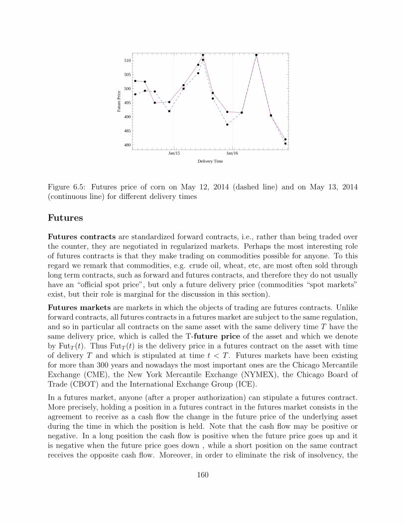
Jan15 Jan16

480

485

490

495

500

505

510

Delivery Time

Futu

rePr

ice

Figure 6.5: Futures price of corn on May 12, 2014 (dashed line) and on May 13, 2014(continuous line) for different delivery times

Futures

Futures contracts are standardized forward contracts, i.e., rather than being traded overthe counter, they are negotiated in regularized markets. Perhaps the most interesting roleof futures contracts is that they make trading on commodities possible for anyone. To thisregard we remark that commodities, e.g. crude oil, wheat, etc, are most often sold throughlong term contracts, such as forward and futures contracts, and therefore they do not usuallyhave an “official spot price”, but only a future delivery price (commodities “spot markets”exist, but their role is marginal for the discussion in this section).

Futures markets are markets in which the objects of trading are futures contracts. Unlikeforward contracts, all futures contracts in a futures market are subject to the same regulation,and so in particular all contracts on the same asset with the same delivery time T have thesame delivery price, which is called the T-future price of the asset and which we denoteby FutT (t). Thus FutT (t) is the delivery price in a futures contract on the asset with timeof delivery T and which is stipulated at time t < T . Futures markets have been existingfor more than 300 years and nowadays the most important ones are the Chicago MercantileExchange (CME), the New York Mercantile Exchange (NYMEX), the Chicago Board ofTrade (CBOT) and the International Exchange Group (ICE).

In a futures market, anyone (after a proper authorization) can stipulate a futures contract.More precisely, holding a position in a futures contract in the futures market consists in theagreement to receive as a cash flow the change in the future price of the underlying assetduring the time in which the position is held. Note that the cash flow may be positive ornegative. In a long position the cash flow is positive when the future price goes up and itis negative when the future price goes down , while a short position on the same contractreceives the opposite cash flow. Moreover, in order to eliminate the risk of insolvency, the

160

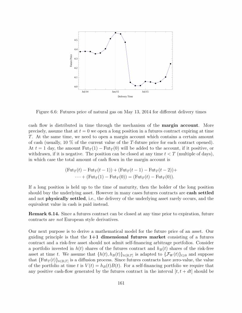
Jul14 Jan15 Jul15

4.0

4.1

4.2

4.3

4.4

4.5

Delivery Time

Futu

rePr

ice

Figure 6.6: Futures price of natural gas on May 13, 2014 for different delivery times

cash flow is distributed in time through the mechanism of the margin account. Moreprecisely, assume that at t = 0 we open a long position in a futures contract expiring at timeT . At the same time, we need to open a margin account which contains a certain amountof cash (usually, 10 % of the current value of the T -future price for each contract opened).At t = 1 day, the amount FutT (1) − FutT (0) will be added to the account, if it positive, orwithdrawn, if it is negative. The position can be closed at any time t < T (multiple of days),in which case the total amount of cash flown in the margin account is

(FutT (t)− FutT (t− 1)) + (FutT (t− 1)− FutT (t− 2))+

· · ·+ (FutT (1)− FutT (0)) = (FutT (t)− FutT (0)).

If a long position is held up to the time of maturity, then the holder of the long positionshould buy the underlying asset. However in many cases futures contracts are cash settledand not physically settled, i.e., the delivery of the underlying asset rarely occurs, and theequivalent value in cash is paid instead.

Remark 6.14. Since a futures contract can be closed at any time prior to expiration, futurecontracts are not European style derivatives.

Our next purpose is to derive a mathematical model for the future price of an asset. Ourguiding principle is that the 1+1 dimensional futures market consisting of a futurescontract and a risk-free asset should not admit self-financing arbitrage portfolios. Considera portfolio invested in h(t) shares of the futures contract and hB(t) shares of the risk-freeasset at time t. We assume that h(t), hB(t)t∈[0,T ] is adapted to FW (t)t≥0 and supposethat FutT (t)t∈[0,T ] is a diffusion process. Since futures contracts have zero-value, the valueof the portfolio at time t is V (t) = hB(t)B(t). For a self-financing portfolio we require thatany positive cash-flow generated by the futures contract in the interval [t, t + dt] should be

161

invested to buy shares of the risk-free asset and that, conversely, any negative cash flowshould be settled by issuing shares of the risk-free asset (i.e., by borrowing money). Sincethe cash-flow generated in the interval [t, t+ dt] is given by dC(t) = h(t)dFutT (t), the valueof a self-financing portfolio invested in the 1+1 dimensional futures market must satisfy

dV (t) = hB(t)dB(t) + h(t)dFutT (t) = R(t)V (t)dt+ h(t)dFutT (t),

or equivalentlydV ∗(t) = h(t)D(t)dFutT (t). (6.113)

Now, we have seen that a simple condition ensuring that a portfolio is not an arbitrageis that its discounted value be a martingale in the risk-neutral measure relative to thefiltration generated by the Brownian motion. By (6.113), the latter condition is achieved by

requiring that dFutT (t) = ∆(t)dW (t), for some stochastic process ∆(t)t∈[0,T ] adapted toFW (t)t∈[0,T ]. In particular, it is reasonable to impose that

(i) FutT (t)t∈[0,T ] should be a P-martingale relative to FW (t)t≥0.

Furthermore, it is clear that the future price of an asset at the expiration date T should beequal to its spot price at time T , and so we impose that

(ii) FutT (T ) = Π(T ).

It follows by Exercise 3.31 that the conditions (i)-(ii) determine a unique stochastic processFutT (t)t∈[0,T ], which is given in the following definition.

Definition 6.6. Assume that the price Π(t)t≥0 of the asset satisfies

dΠ(t) = α(t)Π(t)dt+ σ(t)Π(t)dW (t),

where α(t)t≥0, σ(t)t≥0, R(t)t≥0 ∈ C0[FW (t)] and σ(t) > 0 almost surely for all times.The T -Future price at time t of the asset is the FW (t)t≥0-adapted stochastic processFutT (t)t∈[0,T ] given by

FutT (t) = E[Π(T )|FW (t)], t ∈ [0, T ].

We now show that our goal to make the futures market arbitrage-free has been achieved.

Theorem 6.19. There exists a stochastic process ∆(t)t∈[0,T ] adapted to FW (t)t≥0 suchthat

FutT (t) = FutT (0) +

∫ t

0

∆(s)dW (s). (6.114)

Moreover, any FW (t)t≥0-adapted self-financing portfolio h(t), hB(t)t∈[0,T ] invested in the1+1 dimensional futures market is not an arbitrage.

162

Proof. The second statement follows immediately by the first one, since (6.113) and (6.114)imply that the value of a self-financing portfolio invested in the 1+1 dimensional futuresmarket is a P-martingale relative to the filtration FW (t)t∈[0,T ]. To prove (6.114), we firstnotice that, by (3.24),

Z(s)E[FutT (t)|FW (s)] = E[Z(t)FutT (t)|FW (s)].

By the martingale property of the future price, the left hand side is Z(s)FutT (s). Hence

Z(s)FutT (s) = E[Z(t)FutT (t)|FW (s)],

that is to say, the process Z(t)FutT (t)t∈[0,T ] is a P-martingale relative to the filtrationFW (t)t∈[0,T ]. By the martingale representation theorem, Theorem 4.5(v), there exists astochastic process Γ(t)t∈[0,T ] adapted to FW (t)t≥0 such that

Z(t)FutT (t) = FutT (0) +

∫ t

0

Γ(s)dW (s).

We now proceed as in the proof of Theorem 6.2, namely we write

dFutT (t) = d(Z(t)FutT (t)Z(t)−1)

and apply Ito’s product rule and Ito’s formula to derive that (6.114) holds with

∆(t) = θ(t)FutT (t) +Γ(t)

Z(t).

Exercise 6.35 (Sol. 45). Show that the Forward-Future spread of an asset, i.e., thedifference between its forward and future price, satisfies

ForT (t)−FutT (t) =1

E[D(T )|FW (t)]

E[D(T )Π(T )|FW (t)]−E[D(T )|FW (t)]E[Π(T )|FW (t)]

.

(6.115)Moreover, show that when the interest rate R(t)t∈[0,T ] is a deterministic function of time(e.g., a deterministic constant), then ForT (t) = FutT (t), for all t ∈ [0, T ].

6.8 Multi-dimensional markets

In this section we consider N + 1 dimensional stock markets. We denote the stocks prices by

S1(t)t≥0, . . . , SN(t)t≥0

and assume the following dynamics

dSk(t) =

(µk(t) dt+

N∑j=1

σkj(t)dWj(t)

)Sk(t), (6.116)

163

for some stochastic processes µk(t)t≥0, σkj(t)t≥0, j, k = 1, . . . , N in the class C0[FW (t)],where in this section FW (t)t≥0 denotes the filtration generated by the Brownian motionsW1(t)t≥0, . . . WN(t)t≥0. Moreover we assume that the Brownian motions are indepen-dent, in particular

dWj(t)dWk(t) = 0, for all j 6= k, (6.117)

see Exercise 3.25. Finally R(t)t≥0 ∈ C0[FW (t)] is the interest rate of the money market.

Now, given stochastic processes θk(t)t≥0 ∈ C0[FW (t)], k = 1, . . . , N , satisfying the Novikovcondition (4.20), the stochastic process Z(t)t≥0 given by

Z(t) = exp

(−

N∑k=1

(∫ t

0

1

2θ2k(s) ds+

∫ t

0

θk(s) dWk(s)

))(6.118)

is a martingale relative to the filtration FW (t)t≥0 (see Exercise 4.7). Since E[Z(t)] =E[Z(0)] = 1, for all t ≥ 0, we can use the stochastic process Z(t)t≥0 to define a risk-neutral probability measure associated to the N + 1 dimensional stock market, as we did inthe one dimensional case, see Definition 6.1.

Definition 6.7. Let T > 0 and assume that the market price of risk equations

µj(t)−R(t) =N∑k=1

σjk(t)θk(t), j = 1, . . . , N, (6.119)

admit a solution (θ1(t), . . . , θN(t)), for all t ≥ 0. Define the stochastic process Z(t)t≥0 as

in (6.118). Then the measure P equivalent to P given by

P(A) = E[Z(T )IA]

is called the risk-neutral probability measure of the market at time T .

Note that, as opposed to the one dimensional case, the risk-neutral measure just definedneed not be unique, as the market price of risk equations may admit more than one solution.For each risk-neutral probability measure P we can apply the multidimensional Girsanovtheorem 4.11 and conclude that the stochastic processes W1(t)t≥0, . . . WN(t)t≥0 given by

Wk(t) = Wk(t) +

∫ t

0

θk(s) ds

are P-independent Brownian motions. Moreover these Brownian motions are P-martingalesrelative to the filtration FW (t)t≥0.

Now let hS1(t)t≥0, . . . , hSN (t)t≥0 ∈ C0[FW (t)] be stochastic processes representing thenumber of shares on the stocks in a portfolio invested in the N+1 dimensional stock market.Let hB(t)t≥0 be the number of shares on the risk-free asset. The portfolio value is

V (t) =N∑k=1

hSk(t)Sk(t) + hB(t)B(t)

164

and the portfolio process is self-financing if its value satisfies

dV (t) =N∑k=1

hSk(t)dSk(t) + hB(t)dB(t),

that is

dV (t) =N∑k=1

hSk(t)dSk(t) +R(t)

(V (t)−

N∑k=1

hSk(t)Sk(t)

)dt.

Theorem 6.20. Assume that a risk-neutral probability P exists, i.e., the equations (6.119)admit a solution. Then the discounted value of any self-financing portfolio invested in theN+1 dimensional market is a P-martingale relative to the filtration FW (t)t≥0. In particular(by Theorem 3.15) there exists no self-financing arbitrage portfolio invested in the N + 1dimensional stock market.

Proof. The discounted value of the portfolio satisfies

dV ∗(t) = D(t)

(N∑j=1

hSj(t)Sj(t)(αj(t)−R(t)) dt+N∑

j,k=1

hSj(t)Sj(t)σjk(t)dWk(t)

)

= D(t)

(N∑j=1

hSj(t)Sj(t)N∑k=1

σjk(t)θk(t)dt+N∑

j,k=1

hSj(t)Sj(t)σjk(t)dWk(t)

)

= D(t)N∑j=1

hSj(t)Sj(t)N∑k=1

σjk(t)dWk(t).

All Ito’s integrals in the last line are P-martingales relative to FW (t)t≥0. The resultfollows.

Exercise 6.36. Work out the details of the computations omitted in the proof of the previoustheorem.

Next we show that the existence of a risk-neutral probability measure is necessary for theabsence of self-financing arbitrage portfolios in N + 1 dimensional stock markets.

Let N = 3 and assume that the market parameters are constant. Let R(t) = r > 0,(µ1, µ2, µ3) = (2, 3, 2) and let the volatility matrix be given by

σij =

1 2 02 4 01 2 0

.

Thus the stocks prices satisfy

dS1(t) = (2dt+ dW1(t) + 2dW2(t))S1(t),

dS2(t) = (3dt+ 2dW1(t) + 4dW2(t))S2(t),

dS3(t) = (2dt+ dW1(t) + 2dW2(t))S3(t).

165

The market price of risk equations are

θ1 + 2θ2 = 2− r2θ1 + 4θ2 = 3− rθ1 + 2θ2 = 2− r.

This system is solvable if and only if r = 1, in which case there exist infinitely many solutionsgiven by

θ1 ∈ R, θ2 =1

2(1− θ1).

Hence for r = 1 there exists at least one (in fact, infinitely many) risk-neutral probabilitymeasures, and thus the market is free of arbitrage. To construct an arbitrage portfolio when0 < r < 1, let

hS1(t) =1

S1(t), hS2(t) = − 1

S2(t), hS3(t) =

1

S3(t)

and choose hB(t) such that the portfolio process is self-financing (see Exercise 4.10). Thevalue V (t)t≥0 of this portfolio satisfies

dV (t) = hS1(t)dS1(t) + hS2(t)dS2(t) + hS3(t)dS3(t)

+ r(V (t)− hS1(t)S1(t)− hS2(t)S2(t)− hS3(t)S3(t))dt

= rV (t)dt+ (1− r)dt.Hence

V (t) = V (0)ert +1

r(1− r)(ert − 1)

and this portfolio is an arbitrage, because for V (0) = 0 we have V (t) > 0, for all t > 0.Similarly one can find an arbitrage portfolio for r > 1.

Next we address the question of completeness of N + 1 dimensional stock markets, i.e.,the question of whether any European derivative can be hedged in this market. Consider aEuropean derivative on the stocks with pay-off Y and time of maturity T . For instance, fora standard European derivative, Y = g(S1(T ), . . . SN(T )), for some measurable function g.The risk-neutral price of the derivative is

ΠY (t) = E[Y exp(−∫ T

t

R(s) ds)|FW (t)],

and coincides with the value at time t of any self-financing portfolio invested in the N + 1dimensional market. The question of existence of an hedging portfolio is answered by thefollowing theorem.

Theorem 6.21. Assume that the volatility matrix (σjk(t))j,k=1,...N is invertible, for all t ≥ 0.There exist stochastic processes ∆1(t)t∈[0,T ], . . . ∆N(t)t∈[0,T ], adapted to FW (t)t≥0, suchthat

D(t)ΠY (t) = ΠY (0) +N∑k=1

∫ t

0

∆k(s)dWk(s), t ∈ [0, T ]. (6.120)

166

Let (Y1(t), . . . , YN(t)) be the solution of

N∑k=1

σjk(t)Yj(t) =∆k(t)

D(t). (6.121)

Then the portfolio hS1(t), . . . , hSN (t), hB(t)t∈[0,T ] given by

hSj(t) =Yj(t)

Sj(t), hB(t) = (ΠY (t)−

N∑j=1

hSj(t)Sj(t))/B(t) (6.122)

is self-financing and replicates the derivative at any time, i.e., its value V (t) is equal toΠY (t) for all t ∈ [0, T ]. In particular, V (T ) = ΠY (T ) = Y , i.e., the portfolio is hedging thederivative.

The proof of this theorem is conceptually very similar to that of Theorem 6.2 and is thereforeomitted (it makes use of the multidimensional version of the martingale representation the-orem). Notice that, having assumed that the volatility matrix is invertible, the risk-neutralprobability measure of the market is unique. We now show that the uniqueness of the risk-neutral probability measure is necessary to guarantee completeness. In fact, let r = 1 inthe example considered before and pick the following solutions of the market price of riskequations:

(θ1, θ2) = (0, 1/2), and (θ1, θ2) = (1, 0)

(any other pair of solutions would work). The two corresponding risk-neutral probability

measures, denoted respectively by P and P, are given by

P(A) = E[ZIA] P(A) = E[ZIA], for all A ∈ F ,

whereZ = e−

18T− 1

2W2(T ), Z = e−

12T−W1(T ).

Let A = ω : 12W2(T, ω)−W1(T, ω) < 3

8T. Hence

Z(ω) < Z(ω), for ω ∈ A

and thus P(A) < P(A). Consider a financial derivative with pay-off Q = IA/D(T ). If thereexisted an hedging, self-financing portfolio for such derivative, then, since the discountedvalue of such portfolio is a martingale in both risk-neutral probability measures, we wouldhave

V (0) = E[QD(T )], and V (0) = E[QD(T )]. (6.123)

ButE[QD(T )] = E(IA) = P(A) < P(A) = E(IA) = E[QD(T )]

and thus (6.123) cannot be verified.

167

Multi-assets options

Multi-asset options are options on several underlying assets. Notable examples include rain-bow options, basket options and quanto options.

In the following we discuss options on two stocks in a 2+1 dimensional Black-Scholesmarket, i.e., a market with constant parameters. It follows that

dS1(t) = µ1 S1(t)dt+ σ11S1(t)dW1(t) + σ12S1(t)dW2(t) (6.124a)

dS2(t) = µ2 S2(t)dt+ σ21S2(t)dW1(t) + σ22S2(t)dW2(t), (6.124b)

where the volatility matrix

σ =

(σ11 σ12

σ21 σ22

)is invertible (so that the market is complete). Integrating (6.124) we obtain that (S1(t), S2(t))is given by the 2-dimensional geometric Brownian motion:

S1(t) = S1(0)e(µ1− 12

(σ211+σ2

12))t+σ11W1(t)+σ12W2(t), (6.125a)

S2(t) = S2(0)e(µ2− 12

(σ221+σ2

22))t+σ21W1(t)+σ22W2(t), (6.125b)

or, more concisely,

Sj(t) = Sj(0)e(µj−|σj |

2

2)t+σj ·W (t),

where σj = (σj1, σj2), j = 1, 2, W (t) = (W1(t),W2(t)) and · denotes the standard scalarproduct of vectors.

Theorem 6.22. The random variables S1(t), S2(t) have the joint density

fS1(t),S2(t)(x, y) =e− 1

2t

(log x

S(0) − α1t log yS(0) − α2t

)(σσT )−1

log xS(0) − α1t

log yS(0) − α2t

txy√

(2π)2 det(σσT ), (6.126)

where αj = µj − |σj |2

2, j = 1, 2. Moreover logS1(t), logS2(t) are jointly normally distributed

with mean m = (logS1(0) + α1t, logS2(0) + α2t) and covariant matrix C = tσσT .

Proof. Letting Xi = Wi(t)/√t ∈ N (0, 1), we write the stock prices as

S1(t) = S1(0)eα1t+Y1 , S2(t) = S2(0)eα2t+Y2 ,

whereY1 = σ11

√tX1 + σ12

√tX2, Y2 = σ21

√tX1 + σ22

√tX2.

It follows by Exercise 3.20 that Y1, Y2 are jointly normally distributed with zero mean andcovariant matrix C = tσσT , which proves the second statement in the theorem. To computethe joint density of the stock prices, we notice that

S1(t) ≤ x⇔ Y1 ≤ log

(x

S1(0)

)− α1t, S2(t) ≤ y ⇔ Y2 ≤ log

(y

S2(0)

)− α2t,

168

henceFS1(t),S2(t)(x, y) = FY1,Y2(log

x

S1(0)− α1t, log

y

S2(0)− α2t).

Hence

fS1(t),S2(t)(x, y) = ∂2xyFS1(t),S2(t)(x, y) =

1

xyfY1,Y2(log

x

S1(0)− α1t, log

y

S2(0)− α2t).

Using the joint normal density of Y1, Y2 completes the proof.

Exercise 6.37. Show that the process (6.124) is equivalent, in distribution, to the process

dSi(t) = µiSi(t) dt+ σiSi(t)dW(ρ)i (t), i = 1, 2, (6.127)

where

σi =√σ2i1 + σ2

i2, ρ =σ11σ21 + σ12σ22√

(σ211 + σ2

12)(σ221 + σ2

22)∈ [−1, 1] (6.128)

and where W(ρ)1 (t), W

(ρ)2 (t) are correlated Brownian motions with correlation ρ, i.e.,

dW(ρ)1 (t)dW

(ρ)2 (t) = ρ dt.

TIP: Use Exercise 2.11.

Now let R(t) = r be the constant interest rate of the money market. The solution of themarket price of risk equations (6.119) can be written as

θ =

(θ1

θ2

)= σ−1

(µ1 − rµ2 − r

)=

1

detσ

(σ22 −σ12

−σ21 σ11

)(µ1 − rµ2 − r

),

that is

θ1 =1

detσ[σ22(µ1 − r)− σ12(µ2 − r)], θ2 =

1

detσ[−σ21(µ1 − r) + σ11(µ2 − r)].

Replacing dWi(t) = dWi(t)− θi dt into (6.124) we find

dS1(t) = r S1(t)dt+ σ11S1(t)dW1(t) + σ12S1(t)dW2(t), (6.129a)

dS2(t) = r S2(t)dt+ σ21S2(t)dW1(t) + σ22S2(t)dW2(t). (6.129b)

Note that the discounted price of both stocks is a martingale in the risk-neutral probabilitymeasure, as expected. Moreover the system (6.129) can be integrated to give

Sj(t) = Sj(0)e(r−|σj |

2

2)t+σj ·W (t), (6.130)

where W (t) = (W1(t), W2(t)). As W1(t), W2(t) are independent P-Brownian motions, thejoint distribution of the stock prices in the risk-neutral probability measure is given by (6.126)where now

αi = r − |σj|2

2, i = 1, 2.

169

Next consider a standard European style derivative on the two stocks with pay-off Y =g(S1(T ), S2(T )). The risk-neutral price of the derivative is

ΠY (t) = e−r(T−t)E[g(S1(T ), S2(T ))|FW (t)]. (6.131)

By the Markov property for systems of stochastic differential equations, there exists a func-tion vg : [0, T ]× (0,∞)2 → (0,∞) such that

ΠY (t) = vg(t, S1(t), S2(t)). (6.132)

As in the case of options on one single stock, the pricing function can be computed in twoways: using the joint probability density of the stocks or by solving a PDE.

Black-Scholes price for options on two stocks

We show first how to compute the function vg in (6.132) using the joint probability densityof S1(t), S2(t) derived in Theorem 6.22. We argue as in Section 6.3. By (6.130) we have

Si(T ) = Sj(t)e(r−

|σj |2

2)τ+σj ·(W (T )−W (t)), τ = T − t.

Replacing into (6.131) we obtain

ΠY (t) = e−rτ E[g(S1(t)e(r− |σ1|2

2)τ+σ1·(W (T )−W (t)), S2(t)e(r− |σ2|

2

2)τ+σ2·(W (T )−W (t)))|FW (t)].

As (S1(t), S2(t)) is measurable with respect to FW (t) and W (T ) − W (t) is independent ofFW (t), Theorem 3.14 gives

ΠY (t) = vg(t, S1(t), S2(t)),

where

vg(t, x, y) = e−rτ E[g(xe(r− |σ1|2

2)τ+σ1·(W (T )−W (t)), ye(r− |σ2|

2

2)τ+σ2·(W (T )−W (t)))].

To compute the expectation in the right hand side of the latter equation we use that therandom variables

Y1 = σ1 · (W (T )− W (t)), Y2 = σ2 · (W (T )− W (t))

are jointly normally distributed with zero mean and covariance matrix C = τσσT . Hence

vg(t, x, y) = e−rτ∫R

∫Rg(xe(r− |σ1|

2

2)τ+√τξ, ye(r− |σ2|

2

2)τ+√τη)

exp

(−1

2

(ξ η

)(σσT )−1

(ξη

))2π√

det(σσT )dξ dη.

(6.133)

Definition 6.8. The stochastic process ΠY (t)t∈[0,T ] given by (6.132)-(6.133), is calledthe Black-Scholes price of the standard 2-stocks European derivative with pay-off Y =g(S1(T ), S2(T )) and time of maturity T > 0.

170

Black-Scholes PDE for options on two stocks

Next we show how to derive the pricing function vg by solving a PDE.

Theorem 6.23. Let vg be the (unique) strong solution to the terminal value problem

∂tvg + r(x∂xvg + y∂yvg) +1

2(σ2

11 + σ212)x2∂2

xvg +1

2(σ2

21 + σ222)y2∂2

yvg

+ (σ11σ21 + σ12σ22)xy∂xyvg = r vg, t ∈ (0, T ), x, y > 0, (6.134a)

vg(T, x, y) = g(x, y), x, y > 0. (6.134b)

Then (6.132) holds. The PDE in (6.134) is called the 2-dimensional Black-Scholes PDE.

Proof. By Ito’s formula in two dimensions,

d(e−rtvg) =e−rt(− rvg dt+ ∂tvg dt+ ∂xvg dS1(t) + ∂yvg dS2(t)

+ ∂2xyvg dS1(t)dS2(t) +

1

2∂2xvg dS1(t) dS1(t) +

1

2∂2yvg dS2(t) dS2(t)

).

Moreover, using (6.129),

dS1(t)dS1(t) = (σ211 + σ2

12)S1(t)2 dt

dS2(t)dS2(t) = (σ221 + σ2

22)S2(t)2 dt

dS1(t)dS2(t) = (σ11σ21 + σ12σ22)S1(t)S2(t) dt.

It follows that

d(e−rtvg(t, S1(t), S2(t)) = α(t) dt+ e−rtS1(t)∂xvg(t, S1(t), S2(t)) (σ11 dW1(t) + σ12dW2(t))

+ e−rtS2(t)∂yvg(t, S1(t), S2(t)) (σ21 dW1(t) + σ22dW2(t))

where the drift term is

α(t) =e−rt(− rvg + ∂tvg + r(x∂xvg + y∂yvg)

+1

2(σ2

11 + σ212)x2∂2

xvg +1

2(σ2

21 + σ222)y2∂2

yvg

+ (σ11σ21 + σ12σ22)xy∂xyvg)(t, S1(t), S2(t)) = 0,

due to vg solving (6.134). It follows that the stochastic process e−rtvg(t, S1(t), S2(t))t∈[0,T ]

is a P-martingale relative to FW (t)t≥0, hence, using the terminal condition vg(T ) = g, wehave

e−rT E[g(S1(T ), S2(T ))|FW (t)] = e−rtvg(t, S1(t), S2(t)), t ∈ [0, T ],

which proves (6.132).

171

Hedging portfolio

Finally we derive the formulas for the hedging portfolio for standard 2-stocks Europeanderivatives in Black-Scholes markets.

Theorem 6.24. The numbers of shares hS1(t), hS2(t) in the self-financing hedging portfoliofor the European derivative with pay-off Y = g(S1(T ), S2(T )) and maturity T are given by

hS1(t) = ∂xvg(t, S1(t), S2(t)), hS2(t) = ∂yvg(t, S1(t), S2(t)).

Proof. The discounted value of the derivative satisfies dΠ∗Y (t) = ∆1(t)dW1(t)+∆2(t)dW2(t),where

∆1(t) = e−rt(S1(t)σ11∂xvg + S2(t)σ21∂yvg)(t, S1(t), S2(t))

∆2(t) = e−rt(S1(t)σ12∂xvg + S2(t)σ22∂yvg)(t, S1(t), S2(t))

Letting ∆ = (∆1 ∆2)T , we have ∆/e−rt = σTY , where

Y =

(S1(t)∂xvg(t, S1(t), S2(t))S2(t)∂yvg(t, S1(t), S2(t))

).

Hence by Theorem 6.21, the number of stock shares in the hedging portfolio is hS1(t) =Y1/S1(t) = ∂xvg(t, S1(t), S2(t)), hS2(t) = Y2/S2(t) = ∂yvg(t, S1(t), S2(t)), which concludesthe proof of the theorem.

An example of option on two stocks

Let K,T > 0 and consider a standard European derivative with pay-off

Y =

(S1(T )

S2(T )−K

)+

at time of maturity T . Using (6.130), we can write the risk-neutral price of the derivative as

ΠY (t) = e−rτ E[(

S1(T )

S2(T )−K

)+

|FW (t)

]= e−rτ E

[(S1(t)

S2(t)e(|σ2|

2

2− |σ1|

2

2)τ+(σ1−σ2)·(W (T )−W (t)) −K

)+

|FW (t)

].

Now we write

(σ1 − σ2) · (W (T )− W (t)) =√τ [(σ11 − σ21)G1 + (σ12 − σ22)G2] =

√τ(X1 +X2),

where Gj = (Wj(T )−Wj(t))/√τ ∈ N (0, 1), j = 1, 2, hence Xj ∈ N (0, (σ1j−σ2j)

2), j = 1, 2.In addition, X1, X2 are independent random variables, hence, as shown in Section 3.1, X1+X2

172

is normally distributed with zero mean and variance (σ11− σ21)2 + (σ12− σ22)2 = |σ1− σ2|2.It follows that

ΠY (t) = e−rτ E[(

S1(t)

S2(t)e(|σ2|

2

2− |σ1|

2

2)τ+√τ |σ1−σ2|G) −K

)+

],

where G ∈ N (0, 1). Hence, letting

r =|σ1 − σ2|2

2+

( |σ2|22− |σ1|2

2

)and a = e(r−r)τ , we have

ΠY (t) = ae−rτE[(

S1(t)

S2(t)e(r− |σ1−σ2|

2

2)τ+√τ |σ1−σ2|G −K

)+

]Up to the multiplicative parameter a, this is the Black-Scholes price of a call on a stock withprice S1(t)/S2(t), volatility |σ1 − σ2| and for an interest rate of the money market given byr. Hence, Theorem 6.6 gives

ΠY (t) = a

(S1(t)

S2(t)Φ(d+)−Ke−rτΦ(d−)

):= v(t, S1(t), S2(t)) = u(t,

S1(t)

S2(t)) (6.135)

where

d± =log S1(t)

KS2(t)+ (r ± |σ1−σ2|2

2)τ

|σ1 − σ2|√τ

.

As to the self-financing hedging portfolio, we have hS1(t) = ∂xv(t, S1(t), S2(t)), hS2(t) =∂yv(t, S1(t), S2(t)), j = 1, 2. Therefore, recalling the delta function of the standard Europeancall (see Theorem 6.7), we obtain

hS1(t) =a

S2(t)Φ(d+), hS2(t) = −aS1(t)

S2(t)2Φ(d+).

The same result can be obtained by solving the terminal value problem (6.134). Indeed, theform of the pay-off function of the derivative suggests to look for solutions of (6.134) of theform vg(t, x, y) = u(t, x/y). The function u(t, z) satisfies a standard Black-Scholes PDE in1+1 dimension, whose solution is given as in (6.135). The details are left as an exercise.

Exercise 6.38. Derive (6.135) by solving the terminal value problem (6.134).

Exercise 6.39. A two assets correlation call/put option with maturity T is the standardEuropean derivative with pay-off

Ycall =

(S2(T )−K2)+, if S1(T ) > K1

0 otherwise

Yput =

(K2 − S2(T ))+, if S1(T ) < K1

0 otherwise

173

where K1, K2 > 0 and S1(t), S2(t) are the prices of the underlying stocks. Show that in acomplete 2+1 dimensional Black-Scholes market the price of the call option is

Πcall(t) = S2(t)Φ(y2 + σ2

√τ , y1 + ρ σ2

√τ ; ρ)−K2e

−rτΦ(y2, y1; ρ),

where ρ, σi are given by (6.128), Φ(x, y; ρ) is the standard cumulative joint normal distribu-tion, see (2.12), and

yi =log(Si(t)/Ki) + (r − σ2

i /2)τ)

σi√τ

, i = 1, 2.

Show that when the stock prices are independent, the price of the two-asset correlation calloption is the product of the price of a binary option and of a standard call option. Finallyderive the price of the corresponding put option and establish the put-call parity.

Exercise 6.40. Derive the Black-Scholes price, the Black-Scholes PDE (with the terminalcondition) and the put-call parity for the two-asset Asian geometric call/put option, whosepay-off, for the call, is

Ycall =

(exp

(1

T

∫ T

0

log(S1(t)1/2S2(t)1/2) dt

)−K

)+

.

6.9 Introduction to American derivatives

Before giving the precise definition of fair price for American derivatives, we shall presentsome general properties of these contracts. American derivatives can be exercised at anytime prior or including maturity T . Let Y (t) be the pay-off resulting from exercising thederivative at time t ∈ (0, T ]. We call Y (t) the intrinsic value of the derivative. We consideronly standard American derivatives, for which we have Y (t) = g(S(t)), for some measurablefunction g : R→ R. For instance, g(x) = (x−K)+ for American calls and g(x) = (K − x)+

for American puts. We denote by ΠY (t) the price of the American derivative with intrinsicvalue Y (t) and by ΠY (t) the price of the European derivative with pay-off Y = Y (T ) atmaturity time T (given by (6.10)). Two obvious properties of American derivatives are thefollowing:

(i) ΠY (t) ≥ ΠY (t), for all t ∈ [0, T ]. In fact an American derivative gives to its ownerall the rights of the corresponding European derivative plus one: the option of earlyexercise. Thus it is clear that the American derivative cannot be cheaper than theEuropean one.

(ii) ΠY (t) ≥ Y (t), for all t ∈ [0, T ]. If not, an arbitrage opportunity would arise bypurchasing the American derivative and exercising it immediately.

Any reasonable definition of fair price for American derivatives must satisfy (i)-(ii).

174

Definition 6.9. A time t ∈ (0, T ] is said to be an optimal exercise time for the American

derivative with intrinsic value Y (t) if ΠY (t) = Y (t).

Hence by exercising the derivative at an optimal exercise time t, the buyer takes full advan-tage of the derivative: the resulting pay-off equals the value of the derivative. On the otherhand, if ΠY (t) > Y (t) and the buyer wants to close the (long) position on the Americanderivative, then the optimal strategy is to sell the derivative, thereby cashing the amountΠY (t).

Theorem 6.25. Assume (i) holds and let C(t) be the price of an American call at timet ∈ [0, T ]. Assume further that the underlying stock price follows a generalized geometricBrownian motion and that the interest rate R(t) of the money market is strictly positive for

all times. Then C(t) > Y (t), for all t ∈ [0, T ). In particular it is never optimal to exercisethe call prior to maturity.

Proof. For S(t) ≤ K the claim becomes C(t) > 0 for t ∈ [0, T ), which is obvious (since

C(t) ≥ C(t) > 0). For S(t) > K we write

C(t) ≥ C(t) = E[(S(T )−K)+D(T )/D(t)|FW (t)] ≥ E[(S(T )−K)D(T )/D(t)|FW (t)]

= E[S(T )D(T )/D(t)|FW (t)]−KE[D(T )/D(t)|FW (t)] > D(t)−1E[S∗(T )|FW (t)]−K= S(t)−K = (S(t)−K)+,

where we used D(T )/D(t) < 1 (by the positivity of the interest rate R(t)) and the martingaleproperty of the discounted price S∗(t)t∈[0,T ] of the stock.

It follows that under the assumptions of the previous theorem the earlier exercise optionof the American call is worthless, hence American and European call options with the samestrike and maturity have the same value.

Remark 6.15. The result is valid for general standard American derivatives with convexpay-off function, see [25, Section 8.5].

Remark 6.16. A notable exception to the assumed conditions in Theorem 6.25 is when theunderlying stock pays a dividend. In this case it can be shown that it is optimal to exercisethe American call immediately before the dividend is payed, provided the price of the stockis sufficiently high, see Theorem 6.30 below.

Definition 6.10. Let T ∈ (0,∞). A random variable τ : Ω → [0, T ] is called a stoppingtime for the filtration FW (t)t≥0 if τ ≤ t ∈ FW (t), for all t ∈ [0, T ]. We denote by QT

the set of all stopping times for the filtration FW (t)t≥0.

Think of τ as the time at which some random event takes place. Then τ is a stopping timeif the occurrence of the event before or at time t can be inferred by the information availableup to time t (no future information is required). For the applications that we have in mind,

175

τ will be the optimal exercise time of an American derivative, which marks the event thatthe price of the derivative equals its intrinsic value.

From now on we assume that the market has constant parameters and r > 0. Hence theprice of the stock is given by the geometric Brownian motion

S(t) = S(0)e(r−σ2

2)t+σW (t).

We recall that in this case the price ΠY (0, T ) at time t = 0 of the European derivative withpay-off Y = g(S(T )) at maturity time T > 0 is given by

ΠY (0, T ) = E[e−rTg(S(T ))].

Now, if the writer of the American derivative were sure that the buyer would exercise at thetime u ∈ (0, T ], then the fair price of the American derivative at time t = 0 would be equal toΠY (0, u). As the writer cannot anticipate when the buyer will exercise, we would be temptedto define the price of the American derivative at time zero as maxΠY (0, u), 0 ≤ u ≤ T.However this definition would actually be unfair, as it does not take into account the factthat the exercise time is a stopping time, i.e., it is random and it cannot be inferred usingfuture information. This leads us to the following definition.

Definition 6.11. In a market with constant parameters, the fair price at time t = 0 of thestandard American derivative with intrinsic value Y (t) = g(S(t)) and maturity T > 0 isgiven by

ΠY (0) = maxτ∈QT

E[e−rτg(S(τ))], (6.136)

where S(τ) = S(0)e(r−σ2

2)τ+σW (τ).

It is not possible in general to find an closed formula for the price of American derivatives.A notable exception is the price of perpetual American put options, which we discuss next.

Perpetual American put options

An American put option is called perpetual if it never expires, i.e., T =∞. This is of coursean idealization, but perpetual American puts are very useful to visualize the structure ofgeneral American put options. In this section we follow closely the discussion on [25, Section8.3]. Definition 6.136 becomes the following.

Definition 6.12. Let Q be the set of all stopping times for the filtration FW (t)t≥0, i.e.,τ ∈ Q iff τ : Ω→ [0,∞] is a random variable and τ ≤ t ∈ FW (t), for all t ≥ 0. The fairprice at time t = 0 of the perpetual American put with strike K is

Π(0) = maxτ∈Q

E[e−rτ (K − S(τ))+] (6.137)

where S(τ) = S(0)e(r−σ2

2)τ+σW (τ).

176

Theorem 6.26. There holdsΠ(0) = vL(S(0)), (6.138)

where

vL(x) =

K − x 0 ≤ x ≤ L

(K − L)(xL

)− 2rσ2 x > L

and

L =2r

2r + σ2K.

Before we prove the theorem, some remarks are in order:

(i) L < K;

(ii) For S(0) ≤ L we have Π(0) = vL(S(0)) = K − S(0) = (K − S(0))+. Hence whenS(0) ≤ L it is optimal to exercise the derivative.

(iii) We have Π(0) > (K − S(0))+ for S(0) > L. In fact

v′L(x) = −2r

σ2

(xL

)− 2rσ2−1 K − L

L,

hence v′L(L) = −1. Moreover

v′′L(x) =2r

σ2(2r

σ2+ 1)

(xL

)− 2rσ2−2 K − L

L2,

which is always positive. Thus the graph of vL(x) always lies above K − x for x > L.It follows that it is not optimal to exercise the derivative if S(0) > L.

(iv) In the perpetual case, any time is equivalent to t = 0, as the time left to maturity isalways infinite. Hence

Π(t) = vL(S(t)).

In conclusion the theorem is saying us that the buyer of the derivative should exercise assoon as the stock price falls below the threshold L. In fact we can reformulate the theoremin the following terms:

Theorem 6.27. The maximum of E[e−rτ (K − S(τ))+] over all possible τ ∈ Q is achievedat τ = τ∗, where

τ∗ = mint ≥ 0 : S(t) = L.Moreover E[e−rτ∗(K − S(τ∗))+] = vL(S(0)).

For the proof of Theorem 6.26 we need the optional sampling theorem:

177

Theorem 6.28. Let X(t)t≥0 be an adapted process and τ a stopping time. Let t ∧ τ =min(t, τ). If X(t)t≥0 is a martingale/supermatingale/submartingale, then X(t∧ τ)t≥0 isalso a martingale/supermartingale/submartingale.

We can now prove Theorem 6.26. We divide the proof in two steps, which correspondrespectively to Theorem 8.3.5 and Corollary 8.3.6 in [25].

Step 1: The stochastic process e−r(t∧τ)vL(S(t∧ τ))t≥0 is a super-martingale for all τ ∈ Q.Moreover for S(0) > L the stochastic process e−r(t∧τ∗)vL(S(t∧ τ∗))t≥0 is a martingale. ByIto’s formula,

d(e−rtvL(S(t))) = e−rt[−rvL(S(t)) + rS(t)v′L(S(t)) +1

2σ2S(t)2v′′L(S(t))]dt

+ e−rtσS(t)v′L(S(t))dW (t).

The drift term is zero for S(t) > L and it is equal to −rK dt for S(t) ≤ L. Hence

e−rtvL(S(t)) = vL(S(0))− rK∫ t

0

e−ruIS(u)≤L(u) du+

∫ t

0

e−ruσS(u)v′L(S(u))dW (u).

Since the drift term is non-positive, then e−rtvL(t)t≥0 is a supermartingale and thus by theoptional sampling theorem, the process e−r(t∧τ)vL(S(t ∧ τ)t≥0 is a also a supermartingale,for all τ ∈ Q. Now, if S(0) > L, then, by continuity of the paths of the geometric Brownianmotion, S(u, ω) > L as long as u < τ∗(ω). Hence by stopping the process at τ∗ the stockprice will never fall below L and therefore the drift term vanishes, that is

e−r(t∧τ∗)vL(S(t ∧ τ∗)) = vL(S(0)) +

∫ t∧τ∗

0

e−ruσS(u)v′L(S(u))dW (u).

The Ito integral is a martingale and thus the Ito integral stopped at time τ∗ is also amartingale by the optional sampling theorem. The claim follows.

Step 2: The identity (6.138) holds. The supermartingale property of the process e−r(t∧τ)vL(S(t∧τ))t≥0 implies that its expectation is non-increasing, hence

E[e−r(t∧τ)vL(S(t ∧ τ))] ≤ vL∗(S(0)).

As vL(x) is bounded and continuous, the limit t→ +∞ gives

E[e−rτvL(S(τ))] ≤ vL(S(0)).

As vL(x) ≥ (K − x)+ we also have

E[e−rτ (K − S(τ))+] ≤ vL(S(0)).

178

Taking the maximum over all τ ∈ Q we obtain

Π(0) = maxτ∈Q

E[e−rτ (K − S(τ))+] ≤ vL(S(0)).

Now we prove the reverse inequality Π(0) ≥ vL(S(0)). This is obvious for S(0) ≤ L. In fact,

letting τ = mint ≥ 0 : S(t) ≤ L, we have τ ≡ 0 for S(0) ≤ L and so maxτ∈Q E[e−rτ (K −S(τ))+] ≥ E[e−rτ (K − S(τ))+] = (K − S(0))+ = vL(S(0)), for S(0) ≤ L. For S(0) > Lwe use the martingale property of the stochastic process e−r(t∧τ∗)vL(S(t ∧ τ∗))t≥0, whichimplies

E[e−r(t∧τ∗)vL(S(t ∧ τ∗))] = vL(S(0)).

Hence in the limit t→ +∞ we obtain

vL(S(0)) = E[e−rτ∗vL(S(τ∗))].

Moreover e−rτ∗vL(S(τ∗)) = e−rτ∗vL(L) = e−rτ∗(K − S(τ∗))+, hence

vL(S(0)) = E[e−rτ∗(K − S(τ∗))+].

It follows thatΠ(0) = max

τ∈QE[e−rτ (K − S(τ))+] ≥ vL(S(0)),

which completes the proof. 2

Next we discuss the problem of hedging the perpetual American put with a portfolio investedin the underlying stock and the risk-free asset.

Definition 6.13. A portfolio process hS(t), hB(t)t≥0 is said to be replicating the perpetual

American put if its value V (t)t≥0 equals Π(t) for all t ≥ 0.

Thus by setting-up a replicating portfolio, the writer of the perpetual American put is sureto always be able to afford to pay-off the buyer. Note that in the European case a self-financing hedging portfolio is trivially replicating, as the price of European derivatives hasbeen defined as the value of such portfolios. However in the American case a replicatingportfolio need not be self-financing: if the buyer does not exercise at an optimal exercisetime, the writer must withdraw cash from the portfolio in order to replicate the derivative.This leads to the definition of portfolio generating a cash flow.

Definition 6.14. A portfolio hS(t), hB(t)t≥0 with value V (t)t≥0 is said to generate acash flow with rate c(t) if c(t)t≥0 is adapted to FW (t)t≥0 and

dV (t) = hS(t)dS(t) + hB(t)dB(t)− c(t)dt (6.139)

Remark 6.17. Note that the cash flow has been defined so that c(t) > 0 when the investorwithdraws cash from the portfolio (causing a decrease of its value).

The following theorem is Corollary 8.3.7 in [25].

179

Theorem 6.29. The portfolio given by

hS(t) = v′L(S(t)), hB(t) =vL(S(t))− hS(t)S(t)

B(0)ert

is replicating the perpetual American put while generating the case flow c(t) = rKIS(t)≤L(i.e., cash is withdrawn at the rate rK whenever S(t) ≤ L, provided of course the buyer doesnot exercise the derivative).

Proof. By definition, V (t) = hS(t)S(t) + hB(t)B(t) = vL(S(t)) = Π(t), hence the portfoliois replicating. Moreover

dV (t) = d(vL(S(t))) = hS(t)dS(t) +1

2v′′L(S(t))σ2S(t)2dt. (6.140)

Now, a straightforward calculation shows that vL(x) satisfies

−rvL + rxv′L +1

2σx2v′′L = −rKIx≤L,

a relation which was already used in step 1 in the proof of Theorem 6.26. It follows that

1

2v′′L(S(t))σ2S(t)2dt = r(vL(S(t))− S(t)hS(t))dt− rKIS(t)≤Ldt

= hB(t)dB(t)− rKIS(t)≤Ldt.

Hence (6.140) reduces to (6.139) with c(t) = rKIS(t)≤L, and the proof is complete.

Remarks on American put options with finite maturity

The pricing function vL(x) of perpetual American puts satisfies

− rvL + rxv′L +1

2σ2x2v′′L = 0 when x > L, (6.141)

vL(x) = (K − x), for x ≤ L, v′L(L) = −1. (6.142)

It can be shown that the pricing function of American put options with finite maturitysatisfies a similar problem. Namely, letting P (t) be the fair price at time t of the American

put with strike K and maturity T > t, it can be shown that P (t) = v(t, S(t)), where v(t, x)satisfies

∂tv + rx∂xv +1

2σ2x2∂2

xv = rv, if x > x∗(t), (6.143)

v(t, x) = (K − x), for x ≤ x∗(t), ∂xv(t, x∗(t)) = −1, (6.144)

v(T, x) = (k − x)+, x∗(T ) = K, (6.145)

which is a free-boundary value problem. While a numerical solution of the previousproblem can be found using the finite differences method, the price of the American putoption is most commonly computed using binomial tree-approximations, see for instance [5].

180

American calls on a dividend-paying stock

Let Ca(t, S(t), K, T ) denote the Black-Scholes price at time t of the American call with strikeK and maturity T assuming that the underlying stock pays the dividend aS(t−0 ) at time t0 ∈(0, T ). We denote by Ca(t, S(t), K, T ) the Black-Scholes price of the corresponding Europeancall. We omit the subscript a to denote prices in the absence of dividends. Moreover replacingthe letter C with the letter P gives the price of the corresponding put option. We say thatit is optimal to exercise the American call at time t if its Black-Scholes price at this timeequals the intrinsic value of the call, i.e., Ca(t, S(t), K, T ) = (S(t)−K)+.

Theorem 6.30. Consider the American call with strike K and expiration date T and assumethat the underlying stock pays the dividend aS(t−0 ) at the time t0 ∈ (0, T ). Then

Ca(t, S(t), K, T ) > (S(t)−K)+, for t ∈ [t0, T ),

i.e., it is not optimal to exercise the American call prior to maturity after the dividend ispaid. Moreover, there exists δ > 0 such that, if

S(t−0 ) > max(δ

1− a,K),

then the equalityCa(t

−0 , S(t−0 ), K, T ) = (S(t−0 )−K)+

holds, and so it is optimal to exercise the American call “just before” the dividend is to bepaid.

Proof. For the first claim we can assume (S(t)−K)+ = S(t)−K, otherwise the Americancall is out of the money and so it is clearly not optimal to exercise. By Theorem 6.8 we have

Ca(t, S(t), K, T ) = C(t, S(t), K, T ), Pa(t, S(t), K, T ) = P (t, S(t), K, T ), for t ≥ t0.

Hence, by Theorem 6.6, the put-call parity holds after the dividend is paid:

Ca(t, S(t), K, T ) = Pa(t, S(t), K, T ) + S(t)−Ke−r(T−t), t ≥ t0.

Thus, for t ∈ [t0, T ),

Ca(t, S(t), K, T ) ≥ Ca(t, S(t), K, T ) > S(t)−K = (S(t)−K)+,

where we used that P (t, S(t), K, T ) > 0 and r ≥ 0. This proves the first part of the theorem,i.e., the fact that it is not optimal to exercise the American call prior to expiration after thedividend has been paid. In particular

Ca(t, S(t), K, T ) = Ca(t, S(t), K, T ), for t ≥ t0. (6.146)

Next we show that it is optimal to exercise the American call “just before the dividend ispaid”, i.e., Ca(t

−0 , S(t−0 ), K, T ) = (S(t−0 )−K)+, provided the price of the stock is sufficiently

181

high. Of course it must be S(t−0 ) > K. Assume first that Ca(t−0 , S(t−0 ), K, T ) > S(t−0 )−K;

then, owing to (6.146), Ca(t−0 , S(t−0 ), K, T ) = Ca(t

−0 , S(t−0 ), K, T ) (buying the American call

just before the dividend is paid is not better than buying the European call, since it isnever optimal to exercise the derivative prior to expiration). By Theorem (6.8) we haveCa(t

−0 , S(t−0 ), K, T ) = C(t−0 , (1 − a)S(t−0 ), K, T ) = C(t0, (1 − a)S(t−0 ), K, T ), where for the

latter equality we used the continuity in time of the Black-Scholes price function in theabsence of dividends. Since (1− a)S(t−0 ) = S(t0), then

Ca(t−0 , S(t−0 ), K, T ) > S(t−0 )−K ⇒ Ca(t

−0 , S(t−0 ), K, T ) = C(t0, S(t0), K, T ).

Hence

Ca(t−0 , S(t−0 ), K, T ) > S(t−0 )−K ⇒ C(t0, S(t0), K, T ) > S(t−0 )−K = S(t0)+(1−a)S(t−0 )−K.

Therefore, taking the contrapositive statement,

C(t0, S(t0), K, T ) ≤ S(t0) + (1− a)S(t−0 )−K ⇒ Ca(t−0 , S(t−0 ), K, T ) = S(t−0 )−K. (6.147)

Next we remark that the function x → c(t, x,K, T ) − x is decreasing (since ∆ = ∂xc =Φ(d1) < 1, see Theorem 6.7), and

limx→0+

C(t, x,K, T )− x = 0,

limx→+∞

C(t, x,K, T )− x = limx→+∞

P (t, x,K, T )−Ke−r(T−t) = −Ke−r(T−t),

see Exercise 6.12. Thus if (1 − a)S(t−0 ) − K > −Ke−r(T−t), i.e., S(t−0 ) > (1 − a)−1K(1 −e−r(T−t), there exists ω such that if S(t0) > ω, i.e., S(t−0 ) > ω/(1 − a), then the inequalityC(t0, S(t0), K, T ) ≤ S(t0)+(1−a)S(t−0 )−K holds. It follows by (6.147) that for such valuesof S(t−0 ) it is optimal to exercise the call “at time t−0 ”. Letting δ = max(ω,K(1− e−r(T−t))concludes the proof of the theorem.

182

Appendix A

Numerical projects

A.1 A project on the Asian option

The Asian call option with strike K > 0 and maturity T > 0 is the non-standard European

derivative with pay-off Y =(

1T

∫ T0S(t) dt−K

)+

and similarly one defines the Asian put

option. The Black-Scholes price of the Asian option can be computed numerically either bythe Monte Carlo method or by solving the boundary value problem (6.42) using the finitedifference method. The main purpose of this project is to compare the performance of thetwo methods. For the finite difference approach it is convenient to invert the time directionin the problem (6.42) by changing variable t→ T − t, thereby obtaining the system

− ∂tu+σ2

2(γ(t)− z)2∂2

zu = 0, t ∈ (0, T ), z ∈ R (A.1a)

u(0, z) = z+, limz→−∞

u(t, z) = 0, limz→∞

(u(t, z)− z) = 0, t ∈ (0, T ], (A.1b)

where γ(t) = 1−e−rtrT

.

Part 1

• Write a short introduction on the Asian option, where you should discuss in particularwhy this option has been introduced (you can find plenty of info on the web) and themain differences with the standard call option. Outline the content of the rest of thereport.

• Write a finite difference scheme that solves the PDE (A.1) in the domain (t, z) ∈(0, T ) × (−Z,Z) with the appropriate boundary conditions. Use the Crank-Nicolsonmethod (see Remark 5.11).

Part 2

183

• Write a Matlab function that implements the finite difference scheme derived in Part1. The parameters r, σ,K, T , must appear as input variables of your function.

• Plot the initial price of the Asian call as a function of the volatility σ. Show in theplot that the Asian call is always cheaper than the standard call and less sensitive tovolatility. Run several tests for different values of the parameters. Verify numericallythe validity of the put-call parity.

• Compare the performance of the finite difference method and the Monte Carlo methodto compute the price of Asian options, e.g., by performing speed tests. REM: The testsshould be repeated for different values of the parameters. Present your results usingtables.

Include your matlab codes in an appendix.

A.2 A project on the CEV model

In the CEV (Constant Elasticity Variance) model, the price of the stock option with maturityT > 0 and pay-off Y = g(S(T )) is given by ΠY (t) = e−r(T−t)u(t, S(t)), where S(t) is thestock price at time t and u solves

∂tu+ rx∂xu+σ2

2x2δ∂2

xu = 0, x > 0, t ∈ (0, T ), (A.2)

with the terminal condition u(T, x) = g(x), x > 0. Here r > 0, σ > 0, δ > 0 are constants;see Section 6.5 for a derivation of the model. Actually it is more convenient to work withthe equivalent problem

− ∂tu+ rx∂xu+σ2

2x2δ∂2

xu = 0, x > 0, t ∈ (0, T ), (A.3a)

u(0, x) = g(x), x > 0 (A.3b)

which is obtained by the change of variable t→ T − t in (A.2).

The main purpose of this project is to derive numerically some qualitative properties of theCEV model, such as the implied volatility curve.

Part 1

• Write a short introduction on the CEV model, where you should discuss in particularthe applications of the CEV model (you can find plenty of info on the web) and themain differences with the Black-Scholes model. Outline the content of the rest of thereport.

184

• Write a finite difference scheme for the PDE (A.3a) on the domain (t, x) ∈ (0, T ) ×(0, X) with initial data g(x) at time t = 0 and boundary conditions u(0, t) = uL(t),u(X, t) = uR(t). Use the θ-method.

Part 2

• Write a Matlab function that implements the finite difference scheme derived in Part1 in the case of call/put options. Discuss the choice of the boundary conditions. Theparameters r, σ, δ,X, T , must appear as input variables of your function.

• Compare the finite difference solution for δ = 1 with the exact Black-Scholes solutionand study how the error depends on θ ∈ (0, 1). In the rest of the project fix θ whichminimizes this error. Remark: It is up to you how to define this error, but choosewisely!

• Plot the initial price of call and put options as a function of the initial stock price.Focus on nearly-at-the-money options, say x/K ∈ (3/5, 7/5). Run several tests fordifferent values of the parameters. Discuss possible sources of error and how to removethem. Verify numerically the validity of the put-call parity.

• Assume that the market price of calls with different strikes is given by the CEV model.Let σimp(K) be the instantaneous volatility of the stock for which the Black-Scholesprice of the calls equal the market price. Plot K → σimp(K) and discuss your findings

Include your matlab codes in an appendix.

A.3 A project on interest rate models

The purpose of this project is to construct numerically the yield curve of coupon bondsimplied by the CKLS model (6.87). Recall that the price of the ZCB with maturity T isB(t, T ) = v(t, R(t)), where v(t, x) satisfies (6.88) and the terminal condition v(T, x) = 1.

Part 1

• Write a short introduction on the CKLS model in which in particular you should derivethe pricing PDE (6.88) for ZCB’s using the argument in Theorem 6.13. Outline thecontent of the rest of the report.

• Write a finite difference scheme for the pricing PDE derived in the previous step withthe appropriate initial/boundary conditions for the pricing function of a ZCB. Use theCrank-Nicolson method.

Part 2

185

• Write a Matlab function that implements the finite difference scheme derived in Part1. The parameters of the model should appear as inputs in the function. Compare thefinite difference solution for γ = 0 and γ = 1/2 with the exact solution available forthe Vasicek and CIR model.

• Solve Exercise 6.29 and use the matlab function yield to construct numerically theyield curve implied by the CKLS model. Use different values of the parameters andinvestigate how this affects the shape of the yield curve. Can you reproduce all thetypical profiles found in the market? (see Exercise 6.28)

Include your matlab codes in an appendix.

TIP. See [8] for a discussion on how to find numerically the appropriate boundary conditionsfor the PDE (6.88).

186

Appendix B

Solutions to selected problems

1. Solution to Exercise 1.3. Since an event belongs to the intersection of σ-algebras ifand only if it belongs to each single σ-algebra, the proof of the first statement is trivial. Asan example of two σ-algebras whose union is not a σ algebra, take 1 and 3 of Exercise 1.2.

2. Solution to Exercise 1.6. Since A and Ac are disjoint, we have

1 = P(Ω) = P(A ∪ Ac) = P(A) + P(Ac)⇒ P(Ac) = 1− P(A).

To prove 2 we notice that A∪B is the disjoint union of the sets A \B, B \A and A∩B. Itfollows that

P(A ∪B) = P(A \B) + P(B \ A) + P(A ∩B).

Since A is the disjoint union of A ∩B and A \B, we also have

P(A) = P(A ∩B) + P(A \B)

and similarlyP(B) = P(B ∩ A) + P(B \ A). (B.1)

Combining the three identities above yields the result. Moreover, from (B.1) and assumingA ⊂ B, we obtain P(B) = P(A) + P(B \ A) > P(A), which is claim 3.

3. Solution to Exercise 1.8. Since for all k = 0, . . . , N the number of N -tosses ω ∈ ΩN

having NH(ω) = k is given by the binomial coefficient(N

k

)=

N !

k!(N − k)!,

then ∑ω∈ΩN

P(ω) =∑ω∈ΩN

pNH(ω)(1− p)NT (ω) = (1− p)N∑ω∈ΩN

(p

1− p

)NH(ω)

= (1− p)NN∑k=0

(N

k

)(p

1− p

)k.

187

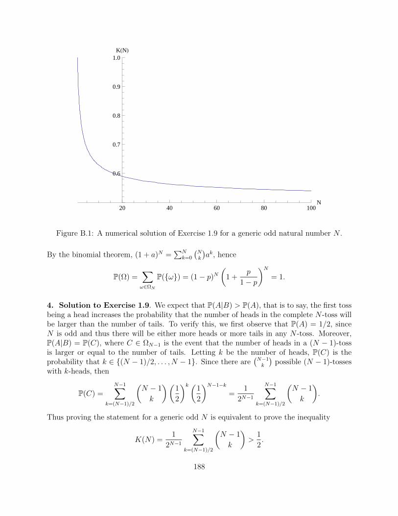
20 40 60 80 100N

0.6

0.7

0.8

0.9

1.0KHNL

Figure B.1: A numerical solution of Exercise 1.9 for a generic odd natural number N .

By the binomial theorem, (1 + a)N =∑N

k=0

(Nk

)ak, hence

P(Ω) =∑ω∈ΩN

P(ω) = (1− p)N(

1 +p

1− p

)N= 1.

4. Solution to Exercise 1.9. We expect that P(A|B) > P(A), that is to say, the first tossbeing a head increases the probability that the number of heads in the complete N -toss willbe larger than the number of tails. To verify this, we first observe that P(A) = 1/2, sinceN is odd and thus there will be either more heads or more tails in any N -toss. Moreover,P(A|B) = P(C), where C ∈ ΩN−1 is the event that the number of heads in a (N − 1)-tossis larger or equal to the number of tails. Letting k be the number of heads, P(C) is theprobability that k ∈ (N − 1)/2, . . . , N − 1. Since there are

(N−1k

)possible (N − 1)-tosses

with k-heads, then

P(C) =N−1∑

k=(N−1)/2

(N − 1

k

)(1

2

)k (1

2

)N−1−k

=1

2N−1

N−1∑k=(N−1)/2

(N − 1

k

).

Thus proving the statement for a generic odd N is equivalent to prove the inequality

K(N) =1

2N−1

N−1∑k=(N−1)/2

(N − 1

k

)>

1

2.

188

A “numerical proof” of this inequality is provided in Figure B.1. Note that the functionK(N) is decreasing and converges to 1/2 as N →∞.

5. Solution to Exercise 2.1. Since Ω = X ∈ R, then Ω ∈ σ(X). X ∈ Uc is the setof sample points ω ∈ Ω such that X(ω) /∈ U . The latter is equivalent to X(ω) ∈ U c, henceX ∈ Uc = X ∈ U c. Since U c ∈ B(R), it follows that X ∈ U ∈ σ(X). Finally we haveto prove that σ(X) is closed with respect to the countable union of sets. Let Akk∈N ⊂ σ(X).By definition of σ(X), there exist Ukk∈N ⊂ B(R) such that Ak = X ∈ Uk. Thus we havethe following chain of equivalent statements

ω ∈ ∪k∈NAk ⇔ ∃k ∈ N : X(ω) ∈ Uk ⇔ X(ω) ∈ ∪k∈NUk ⇔ ω ∈ X ∈ ∪k∈NUk.Hence ∪k∈NAk = X ∈ ∪k∈NUk. Since ∪k∈NUk ∈ B(R), then ∪k∈NAk ∈ σ(X).

6. Solution to Exercise 2.2. Let A be an event that is resolved by both variables X, Y .This means that there exist I, J ⊆ R such that A = X ∈ I = Y ∈ J. Hence, using theindependence of X, Y ,

P(A) = P(A ∩ A) = P(X ∈ I, Y ∈ J) = P(X ∈ I)P(Y ∈ J) = P(A)P(A) = P(A)2.

Therefore P(A) = 0 or P(A) = 1. Now let a, b be two deterministic constants. Note that, forall I ⊂ R,

P(a ∈ I) =

1 if a ∈ I0 otherwise

and similarly for b. Hence

P(a ∈ I, b ∈ J) =

1 if a ∈ I and b ∈ J0 otherwise

= P(a ∈ I)P(b ∈ J).

Finally we show that X and Y = g(X) are independent if and only if Y is a deterministicconstant. For the “if” part we use that

P(a ∈ I,X ∈ J) =

P(X ∈ J) if a ∈ I0 otherwise

= P(a ∈ I)P(X ∈ J).

For the “only if” part, let z ∈ R and I = g(X) ≤ z = X ∈ g−1(−∞, z]. Then, usingthe independence of X and Y = g(X),

P(g(X) ≤ z) = P(g(X) ≤ z, g(X) ≤ z) = P(X ∈ g−1(−∞, z], g(X) ≤ z)

= P(X ∈ g−1(−∞, z])P(g(X) ≤ z) = P(g(X) ≤ z)P(g(X) ≤ z).

Hence P(Y ≤ z) is either 0 or 1, which implies that Y is a deterministic constant.

7. Solution to Exercise 2.4. A ∈ σ(f(X)) if and only if A = f(X) ∈ U, for someU ∈ B(R). The latter is equivalent to X(ω) ∈ f ∈ U, hence A = X ∈ f ∈ U.Similarly, B = Y ∈ g ∈ V , for some V ∈ B(R). Hence

P(A ∩B) = P(X ∈ f ∈ U ∩ Y ∈ g ∈ V ).As X and Y are independent, the right hand side is equal to P(X ∈ f ∈ U)P(Y ∈g ∈ V ), hence P(A ∩B) = P(A)P(B), as claimed.

189

8. Solution to Exercise 2.6. Write (−∞, b] as the disjoint union of the sets (−∞, a] and(a, b]. Hence also X ∈ (−∞, a], X ∈ (a, b] are disjoint. It follows that

P(−∞ < X ≤ b) = P(−∞ < X ≤ a) + P(a < X ≤ b),

that is, F (b) = F (a) + P(a < X ≤ b), by which the claim follows. To establish that FX isright-continuous we now show that

P(X ≤ x0 +1

n)→ P(X ≤ x0) as n→∞, for all x0 ∈ R.

By the first part of the exercise it suffices to show that P(x0 < x ≤ x0 + 1n)→ 0 as n→∞.

The intervals An = (x0, x0 + n−1] satisfy An+1 ⊂ An and ∩nAn = ∅. Hence by Exercise 1.7we have limn→∞ P(An) = P(∅) = 0. The fact that FX is non-decreasing is obvious. Theproperties limx→∞ FX(x) = 1 and limx→−∞ FX(x) = 0 are also obvious.

9. Solution Exercise 2.7. One way to solve this exercise is to set Ω = R, F = B(R),X(ω) = ω, define the probability of the open interval (a, b) as P((a, b)) = F (b) − F (a) andthen use Caratheodory’s theorem to extend this definition to a probability measure on thewhole B(R). Moreover P(X ≤ x) = P(ω < x) = P((−∞, x)) = F (x).

10. Solution to Exercise 2.8. We first compute the distribution function FY of Y = X2.Clearly, FY (y) = P(X2 ≤ y) = 0, if y ≤ 0. For y > 0 we have

FY (y) = P(X2 ≤ y) = P(−√y < X <√y) =

1√2π

∫ √y−√y

e−x2/2 dx.

Hence, for y > 0,

fY (y) =d

dyFY (y) =

1√2π

(e−y/2

d

dy(√y)− e−y/2 d

dy(−√y)

)=

1√2π

e−y/2√y.

Since Γ(1/2) =√π, this is the claim.

11. Solution to Exercise 2.11. A 2× 2 symmetric matrix

C =

(a bb c

)is positive definite if and only if TrC = a + c > 0 and detC = ac − b2 > 0. In particular,a, c > 0. Let us denote

a = σ21, c = σ2

2, ρ =b

σ1σ2

.

Note that ρ2 = b2

ac< 1. Thus

C =

(σ2

1 σ1σ2ρσ1σ2ρ σ2

2

),

190

and so

C−1 =1

1− ρ2

(1σ2

1− ρσ1σ2

− ρσ1σ2

1σ2

2

).

Substituting into (2.9) proves (2.10).

12. Solution to Exercise 2.12. X ∈ N (0, 1) means that X has density

fX(x) =1√2πe−

x2

2 ,

while Y ∈ E(1) means that Y has density

fY (y) = e−yIy≥0.

Since X, Y are independent, they have the joint density fX,Y (x, y) = fX(x)fY (y). Hence

P(X ≤ Y ) =

∫∫x≤y

fX,Y (x, y) dx dy =

∫Rdx e−

x2

2

∫ ∞x

dy1√2πe−yIy≥0.

To compute this integral, we first divide the domain of integration on the variable x in x ≤ 0and x ≥ 0. So doing we have

P(X ≤ Y ) =1√2π

∫ 0

−∞dx e−

x2

2

∫ ∞0

dy e−y +1√2π

∫ ∞0

dx e−x2

2

∫ ∞x

dy e−y.

Computing the integrals we find

P(X ≤ Y ) =1

2+ e1/2(1− Φ(1)),

where Φ(z) = 1√2π

∫ z−∞ e

−y2/2dy is the standard normal distribution.

13. Solution to Exercise 2.15. The density of S(t) is given by

fS(t)(x) =d

dxFS(t)(x),

provided the distribution FS(t), i.e.,

FS(t)(x) = P(S(t) ≤ x)

is differentiable. Clearly, fS(t)(x) = FS(t)(x) = 0, for x < 0. For x > 0 we use that

S(t) ≤ x if and only if W (t) ≤ 1

σ

(log

x

S(0)− αt

):= A(x).

Thus,

P(S(t) ≤ x) = P(−∞ < W (t) ≤ A(x)) =1√2πt

∫ A(x)

−∞e−

y2

2t dy,

191

where for the second equality we used that W (t) ∈ N(0, t). Hence

fS(t)(x) =d

dx

(1√2πt

∫ A(x)

−∞e−

y2

2t dy

)=

1√2πt

e−A(x)2

2tdA(x)

dx,

for x > 0, that is

fS(t)(x) =1√

2πσ2t

1

xexp

−(log x− logS(0)− αt)2

2σ2t

Ix>0.

Since ∫ ∞0

fS(t)(y)dy = 1,

then p0 = P(S(t) = 0) = 0.

14. Solution to Exercise 3.1. Let X be a binomial random variable. Then

E[X] =N∑k=1

kP(X = k) =N∑k=1

k

(N

k

)pk(1− p)N−k = (1− p)N−1p

N∑k=0

k

(N

k

)( p

1− p)k−1

.

Now, by the binomial theorem

N∑k=0

(N

k

)xk = (1 + x)N ,

for all x ∈ R. Differentiating with respect to x we get

N∑k=0

k

(N

k

)xk−1 = N(1 + x)N−1,

Letting x = p/(1− p) in the last identity we find E[X] = Np.

15. Solution to Exercise 3.3. If Y = 0 almost surely, the claim is obvious. Hence wemay assume that E[Y 2] > 0. Let

Z = X − E[XY ]

E[Y 2]Y.

Then

0 ≤ E[Z2] = E[X2]− E[XY ]2

E[Y 2],

by which (3.3) follows.

16. Solution to Exercise 3.5. The first and second properties follow by the linearity of

192

the expectation. In fact

Var[αX] = E[α2X2]− E[αX]2 = α2E[X2]− α2E[X]2 = α2Var[X],

and

Var[X + Y ] = E[(X + Y )2]− E[X + Y ]2 = E[X2] + E[Y 2] + 2E[XY ]

− E[X]2 − E[Y ]2 − 2E[X]E[Y ] = Var[X] + Var[Y ] + 2Cov(X, Y ).

For the third property, let a ∈ R and compute, using 1 and 2,

Var[Y − aX] = a2Var[X] + Var[Y ]− 2aCov(X, Y ).

Since the variance of a random variable is always non-negative, the parabola y(a) = a2Var[X]+Var[Y ]−2aCov(X, Y ) must always lie above the a-axis, or touch it at one single point a = a0.Hence

Cov(X, Y )2 − Var[X]Var[Y ] ≤ 0,

which proves the first part of the claim 3. Moreover Cov(X, Y )2 = Var[X]Var[Y ] if and onlyif there exists a0 such that Var[−a0X + Y ] = 0, i.e., Y = a0X + b0 almost surely, for someconstant b0. Substituting in the definition of covariance, we see that Cov(X, a0X + b0) =a0Var[X], by which the second claim of property 3 follows immediately.

17. Solution Exercise 3.8. By linearity of the expectation,

E[Wn(t)] =1√nE[M[nt]] = 0,

where we used the fact that E[Xk] = E[Mk] = 0. Since Var[Mk] = k, we obtain

Var[Wn(t)] =[nt]

n.

Since nt ∼ [nt], as n→∞, then limn→∞Var[Wn(t)] = t. As to the covariance of Wn(t) andWn(s) for s 6= t, we compute

Cov[Wn(t),Wn(s)] = E[Wn(t)Wn(s)]− E[Wn(t)]E[Wn(s)] = E[Wn(t)Wn(s)]

= E[

1√nM[nt]

1√nM[ns]

]=

1

nE[M[nt]M[ns]]. (B.2)

Assume t > s (a similar argument applies to the case t < s). If [nt] = [ns] we haveE[M[nt]M[ns]] = Var[M[ns]] = [ns]. If [nt] ≥ 1 + [ns] we have

E[M[nt]M[ns]] = E[(M[nt]−M[ns])M[ns]]+E[M2[ns]] = E[M[nt]−M[ns]]E[M[ns]]+Var[M[ns]] = [ns],

where we used that the increment M[nt]−M[ns] is independent of M[ns]. Replacing into (B.2)we obtain

Cov[Wn(t),Wn(s)] =[ns]

n.

It follows that limn→∞Cov[Wn(t),Wn(s)] = s.

193

18. Solution to Exercise 3.11. We have

E[X] =

∫Rλxe−λxIx≥0 dx = λ

∫ ∞0

xe−λx dx =1

λ,

and

Var[X] = E[X2]− E[X]2 =

∫Rλx2e−λxIx≥0 dx−

1

λ2

= λ

∫ ∞0

x2e−λx dx− 1

λ2=

2

λ2− 1

λ2=

1

λ2.

19. Solution to Exercise 3.12. According to Theorem 3.3, to prove that P is equivalentto P we have to show that E[Z] = 1. Using the density of exponential random variables wehave

E[Z] =λ

λE[e−(λ−λ)X ] =

λ

λ

∫ ∞0

e−(λ−λ)xλe−λx dx = 1.

To show that X ∈ E(λ) in the probability measure P we compute

P(X ≤ x) = E[ZIX≤x] =λ

λE[e−(λ−λ)XIX≤x] =

λ

λ

∫ x

0

e−(λ−λ)yλe−λy dy = 1− e−λx.

20. Solution to Exercise 3.28. We have E[Err] = E[X] − E[E[X|G]] = 0, by Theo-rem 3.13(i). Let Y be G-measurable and set µ = E[Y −X]. Then

Var[Y −X] = E[(Y −X − µ)2] = E[(Y −X − µ+ E[X|G]− E[X|G])2]

= E[(E[X|G]−X)2 + (Y − µ− E[X|G])2 + 2(E[X|G]−X)(Y − µ− E[X|G])

]= Var[Err] + E[α] + 2E[β],

where α = (Y −µ−E[X|G])2 and β = (E[X|G]−X)(Y −µ−E[X|G]). As E[α] ≥ 0 we haveVar[Y −X] ≥ Var[Err] + 2E[β]. Furthermore, as Y − µ− E[X|G] is G-measurable, then

E[β] = E[E[β|G]] = E[(Y − µ− E[X|G])E[(E[X|G]−X)|G] = 0.

Hence Var[Y −X] ≥ Var[Err], for all G-measurable random variables Y .

21. Solution to Exercise 3.30. First we observe that claim (i) follows by claim (ii). Infact, if the compound Poisson process is a martingale, then

E[N(t)− λt|FN(s)] = N(s)− λs, for all 0 ≤ s ≤ t,

by which it follows that

E[N(t)|FN(s)] = N(s) + λ(t− s) ≥ N(s), for all 0 ≤ s ≤ t.

Hence it remains to prove (ii). We have

E[N(t)− λt|FN(s)] = E[N(t)−N(s) +N(s)− λt|FN(s)]

= E[N(t)−N(s)|FN(s)] + E[N(s)|FN(s)]− λt= E[N(t)−N(s)] +N(s)− λt = λ(t− s) +N(s)− λt = N(s)− λs.

194

22. Solution to Exercise 3.32. Taking the conditional expectation of both sides of (3.25)with respect to the event X(s) = x gives (3.27).

23. Solution to Exercise 4.3. Assume

Xi(t) = αit+ σidW (t), i = 1, 2,

for constants α1, α2, σ1, σ2. Then the right hand side of (4.15) is∫ t

0

[(α2s+ σ2W (s))σ1 + (α1s+ σ1W (s))σ2]dW (s)

+

∫ t

0

[(α2s+ σ2W (s))α1 + (α1s+ σ1W (s))α2 + σ1σ2]ds

= σ1

∫ t

0

(α2s+ σ2W (s))dW (s) + σ2

∫ t

0

(α1s+ σ1W (s))dW (s)

+ α1α2t2

2+ α1σ2

∫ t

0

W (s)ds+ α1α2t2

2+ σ1α2

∫ t

0

W (s)ds+ σ1σ2t

= σ1α2

∫ t

0

sdW (s) + 2σ1σ2

∫ t

0

W (s)dW (s) + σ2α1

∫ t

0

sdW (s)

+ α1α2t2 + σ1σ2t+ (α1σ2 + σ1α2)

∫ t

0

W (s)ds

= 2σ1σ2(W (t)2

2− t

2) + σ1σ2t+ α1α2t

2 + (σ1α2 + α1σ2)(

∫ t

0

sdW (s) +

∫ t

0

W (s)ds)

= σ1σ2W (t)2 + α1α2t2 + (σ1α2 + α1σ2)tW (t)

= (α1t+ σ1W (t))(α2t+ σ2W (t)) = X1(t)X2(t).

24. Solution to Exercise 4.4. We have

Cor(W1(t),W2(t)) =E[W1(t)W2(t)]√

Var[W1(t)]Var[W2(t)]=

1

tE[W1(t)W2(t)].

Hence we have to show that E[W1(t)W2(t)] = ρt. By Ito’s product rule

d(W1(t)W2(t)) = W1(t)dW2(t)+W2(t)dW1(t)+dW1(t)dW2(t) = W1(t)dW2(t)+W2(t)dW1(t)+ρdt.

Taking the expectation we find E[W1(t)W2(t)] = ρt, which concludes the first part of theexercise. As to the second part, the independent random variables W1(t),W2(s) have thejoint density

fW1(t)W2(s)(x, y) = fW1(t)(x)fW2(s)(y) =1

2π√tse−

x2

2t− y

2

2s .

Hence

P(W1(t) > W2(s)) =1

2π√ts

∫x>y

e−x2

2t− y

2

2s dx dy =1

2.

195

25. Solution to Exercise 4.5. To solve the exercise we must prove that dX(t) =Γ(t)dW (t), for some process Γ(t)t≥0 adapted to FW (t)t≥0. In fact, by Ito’s formula,

dX(t) = −3W (t) dt+ (3W (t)− 3t) dW (t) +1

26W (t)dW (t)dW (t) = 3(W (t)2 − t)dW (t),

where in the last step we used that dW (t)dW (t) = dt.

26. Solution to Exercise 4.6. By Ito’s formula, the stochastic process Z(t)t≥0 satisfies

dZ(t) = −θ(t)Z(t)dW (t),

which is the claim.

27. Solution to Exercise 4.8. Since I(t)t≥0 is a martingale, then E[I(t)] = E[I(0)] = 0.By Ito’s isometry,

Var[I(t)] = E[Y (t)2] = E[

∫ t

0

A(s)2 ds] =

∫ t

0

A2(s) ds,

since A(t) is not random. To prove that I(t) is normally distributed, it suffices to show thatits characteristic function satisfies

θI(t)(u) = e−u2

2

∫ t0 A(s) ds,

see Section 3.1. The latter is equivalent to

E[eiuI(t)] = e−u2

2

∫ t0 A(s) ds, i.e., E[exp(iuI(t) +

u2

2

∫ t

0

A(s) ds)] = 1.

Let Z(t) = exp(iuI(t) + u2

2

∫ t0A(s) ds). If we show that Z(t) is a martingale, we are done,

because then E[Z(t)] = E[Z(0)] = 1. We write

Z(t) = eiX(t)+Y (t) = f(X(t), Y (t)), X(t) = u

∫ t

0

A(s) dW (s), Y (t) =u2

2

∫ t

0

A2(s) ds.

Then, by Theorem 4.8, using dX(t)dY (t) = dY (t)dY (t) = 0,

dZ(t) = ieiX(t)+Y (t)dX(t) + eiX(t)+Y (t)dY (t)− 1

2eiX(t)+Y (t)dX(t)dX(t) = iuZ(t)A(t)dW (t),

where we used that dX(t)dX(t) = u2A2(t)dt. Being an Ito’s integral, the process Z(t)t≥0

is a martingale, which completes the solution of the exercise.

28. Solution to Exercise 4.10. We have

dV (t) = d(hS(t))S(t) + hS(t)dS(t) + dhS(t)dS(t) + d(hB(t))B(t) + hB(t)dB(t)

where we used that dhB(t)dB(t) = R(t)B(t)dhB(t)dt = 0. Hence dV (t) = hS(t)dS(t) +hB(t)dB(t) holds by letting d(hB(t)) = −B(t)−1[dhS(t)dS(t) + hS(t)dS(t)].

196

29. Solution to Exercise 5.3. The SDE in question is

dX(t) = (a+ bX(t)) dt+ γdW (t), t ≥ s, X(s) = x.

Letting Y (t) = e−btX(t) and applying Ito’s formula we find that Y (t) satisfies

dY (t) = ae−bt dt+ γe−btdW (t), Y (s) = xe−bs.

Hence

Y (t) = xe−bs + a

∫ t

s

e−bu dτ + γ

∫ t

s

e−bu dW (u)

and so

X(t; s, x) = xeb(t−s) − a

b(1− eb(t−s)) +

∫ t

s

γeb(t−u)dW (u).

Taking the expectation we obtain immediately that E[X(t; s, x)] = m(t− s, x). Moreover byExercise 4.8, the Ito integral in X(t; s, x) is a normal random variable with zero mean andvariance ∆(t− s)2, hence the claim follows.

30. Solution to Exercise 5.4. Letting Y (t) = e−t2

2 X(t), we find that dY (t) = e−t2

2 dW (t)and Y (0) = 1. Thus

X(t) = et2

2 + et2

2

∫ t

0

e−u2

2 dW (u).

Note that X(t) is normally distributed with mean

E[X(t)] = et2

2 .

It follows that Cov(X(s), X(t)) = E[X(s)X(t)]− E[X(s)]E[X(t)] is

Cov(X(s), X(t)) = es2+t2

2 E[ ∫ s

0

e−u2

2 dW (u)

∫ t

0

e−u2

2 dW (u)].

Assume for example that s ≤ t. Hence

Cov(X(s), X(t)) = es2+t2

2 E[ ∫ t

0

I[0,s]e−u

2

2 dW (u)

∫ t

0

e−u2

2 dW (u)].

Using the result of Exercise 4.2 we have

Cov(X(s), X(t)) = es2+t2

2

∫ t

0

I[0,s]e−u

2

2 e−u2

2 du = es2+t2

2

∫ s

0

e−u2

du

=√πe

s2+t2

2

∫ √2s

0

e−u2

2du√2π

=√πe

s2+t2

2 (Φ(√

2s)− 1

2).

For general s, t ≥ 0 we find

Cov(X(s), X(t)) =√πe

s2+t2

2 (Φ(√

2 min(s, t))− 1

2).

197

31. Solution to Exercise 6.2. We have, for t ≤ t∗,

ΠZ(t) = D(t)−1E[D(t∗)ΠY (t∗)|FW (t)] = D(t)−1D(t)ΠY (t) = ΠY (t),

where we used the martingale property of the discounted price of the derivative with pay-offY , see Theorem 6.2.

32. Solution to Exercise 6.7. The pay-off function is g(z) = k + z log z. Hence theBlack-Scholes price of the derivative is ΠY (t) = v(t, S(t)), where

v(t, x) = e−rτ∫Rg

(xe

(r−σ

2

2

)τ+σ√τy

)e−

y2

2dy√2π

= e−rτ∫R

(k + xe(r−σ

2

2)τ+σ

√τy(log x+ (r − σ2

2)τ + σ

√τy)

)e−

y2

2dy√2π

= ke−rτ + x log x

∫Re−

12

(y−σ√τ)2 dy√

2π

+ x(r − σ2

2)τ

∫Re−

12

(y−σ√τ)2 dy√

2π+ xσ

√τ

∫Rye−

12

(y−σ√τ)2 dy√

2π

Using that ∫Re−

12

(y−σ√τ)2 dy√

2π= 1,

∫Rye−

12

(y−σ√τ)2 dy√

2π= σ√τ ,

we obtain

v(t, x) = ke−rτ + x log x+ x(r +σ2

2)τ.

Hence

ΠY (t) = ke−rτ + S(t) logS(t) + S(t)(r +σ2

2)τ.

This completes the first part of the exercise. The number of shares of the stock in the hedgingportfolio is given by

hS(t) = ∆(t, S(t)),

where ∆(t, s) = ∂v∂x

= log x+ 1 + (r + σ2

2)τ . Hence

hS(t) = 1 + (r +σ2

2)τ + logS(t).

The number of shares of the bond is obtained by using that

ΠY (t) = hS(t)S(t) +B(t)hB(t),

hence

hB(t) =1

B(t)(ΠY (t)− hS(t)S(t))

= e−rt(ke−rτ + S(t) logS(t) + S(t)(r +σ2

2)τ − S(t)− S(t)(r +

σ2

2)τ − S(t) logS(t))

= ke−rT − S(t)e−rt.

198

This completes the second part of the exercise. To compute the probability that Y > 0,we first observe that the pay-off function g(z) has a minimum at z = e−1 and we haveg(e−1) = k − e−1. Hence if k ≥ e−1, the derivative has probability 1 to expire in the money.If k < e−1, there exist a < b such that

g(z) > 0 if and only if 0 < z < a or z > b.

Hence for k < e−1 we have

P(Y > 0) = P(S(T ) < a) + P(S(T ) > b).

Since S(T ) = S(0)eαT−σ√TG, with G ∈ N(0, 1), then

S(T ) < a⇔ G >log S(0)

a+ αT

σ√T

:= A, S(t) > b⇔ G <log S(0)

b+ αT

σ√T

:= B.

Thus

P(Y > 0) = P(G > A) + P(G < B) =

∫ +∞

A

e−x2

2dx√2π

+

∫ B

−∞e−

x2

2dx√2π

= 1− Φ(A) + Φ(B).

This completes the solution of the third part of the exercise.

33. Solution to Exercise 6.8.The pay-off is

Y c = LH(S(T )−K), for the cash-settled binary call option,

Zc = S(T )H(S(T )−K), for the physically-settled binary call option,

Y p = LH(K − S(T )), for the cash-settled binary put option,

Zp = S(T )H(K − S(T )), for the physically-settled binary put option.

The Black-Scholes price in all cases is given by v(t, S(t)), where v(t, x) is the price functionof the derivative given by (6.19b). Replacing g(z) = LH(z −K) into (6.19b) we obtain

v(t, x) =e−rτ√

2πL

∫RH(xe(r−σ

2

2)τeσ

√τ y −K)e−

y2

2 dy

=e−rτ√

2πL

∫ ∞−d2

e−y2

2 dy = e−rτLΦ(d2) (cash-settled binary call),

where we recall that d2 = 1σ√τ[log(x/K) + (r − σ2

2)τ ]. Similarly, using the pay-off function

g(x) = xH(x−K), one finds that the price function for the physically-settled binary optionis

v(t, x) = xΦ(d1) (physically-settled binary call),

where we recall that d1 = d2 + σ√τ . For the put options one obtains

v(t, x) =

Le−rτΦ(−d2) (cash-settled put),xΦ(−d1) (physically-settled put).

199

Hence, using Φ(z) + Φ(−z) = 1, the following put-call parity relations hold:

ΠY c(t) + ΠY p(t) = Le−rτ , ΠZc(t) + ΠZp(t) = S(t).

The number of shares of the stock in the hedging portfolio is given by hS(t) = ∆(t, S(t)),where ∆(t, x) = ∂v(t, x), hence

∆(t, x) =

Le−rτφ(d2)

xσ√τ

(cash-settled call),

Φ(d1) + φ(d1)σ√τ

(physically settled call),

and similarly for the put options. In any case the number of shares of the risk-free asset inthe hedging portfolio is hB(t) = B(t)−1[v(t, S(t))−∆(t, S(t))S(t)].

34. Solution to Exercise 6.9. The pay-off at time T1 for this derivative is

Y = max(C(T1, S(T1), K, T2), P (t1, S(T1), K, T2)).

Using the identity max(a, b) = a+ max(0, b− a) we obtain

Y = C(T1, S(T1), K, T2) + max(0, P (t1, S(T1), K, T2)− C(t1, S(T1), K, T2)).

By the put-call parity,

Y = C(T1, S(T1), K, T2) + max(0, Ke−r(T2−T1) − S(T1)) = Z + U. (B.3)

Hence ΠY (t) = ΠZ(t) + ΠU(t). Since U is the pay-off of a put option with strike Ke−r(T2−T1)

expiring at time T1 then

ΠU(t) = P (t, S(t), Ke−r(T2−T1), T1). (B.4)

Applying the result of Exercise 6.2 with Z = C(T1, S(T1), K, T2) = Π(S(T2)−K)+(T1) we obtain

ΠZ(t) = C(t, S(t), K, T2). (B.5)

Replacing (B.4) and (B.5) into (B.3) we finally obtain, for the Black-Scholes price of thechooser option,

ΠY (t) = C(t, S(t), K, T2) + P (t, S(t), Ke−r(T2−T1), T1).

35. Solution to Exercise 6.10. First we note that for t ≥ s, we can consider the derivativeas a standard call option with maturity T and known strike price K = S(s), hence

ΠY (t) = C(t, S(t), S(s), T ), for t ≥ s,

where C(t, x,K, T ) is the Black-Scholes price function of the standard call option with strikeK and maturity T . For t < s we write

ΠY (t) = e−r(T−t)E[(S(T )− S(s))+|FW (t)]

= e−r(T−t)E[S(t)(e(r− 12σ2)(T−t)+σ(W (T )−W (t)) − e(r− 1

2σ2)(s−t)+σ(W (s)−W (t)))+|FW (t)]

= e−r(T−t)S(t)E[(e(r− 12σ2)(T−t)+σ(W (T )−W (t)) − e(r− 1

2σ2)(s−t)+σ(W (s)−W (t)))+]

200

where in the last step we used that S(t) is measurable with respect to FW (t) and that theBrownian motion increments are independent of FW (t). It follows that

ΠY (t) = e−r(T−t)S(t)E[e(r− 12σ2)(s−t)+σ(W (s)−W (t))(e(r− 1

2σ2)(T−s)+σ(W (T )−W (s)) − 1)+]

= e−r(T−t)S(t)E[e(r− 12σ2)(s−t)+σ(W (s)−W (t))]E[(e(r− 1

2σ2)(T−s)+σ(W (T )−W (s)) − 1)+]

where in the last step we used that the two Brownian motion increments are independent.Computing the expectations using that W (t2) −W (t1) ∈ N (0, t2 − t1), for all t2 > t1, wefind

ΠY (t) = S(t)(Φ(a+ σ√T − t)− e−r(T−s)Φ(a)), a =

(r − 12σ2)√T − s

σ

This completes the solution to the first part of the exercise. As to the put call parity, letZ = (S(s)− S(T ))+. As (x− y)+ − (y − x)+ = x− y, we have

ΠY (t)− ΠZ(t) = e−r(T−t)E[(S(T )− S(s))+|FW (t)]− e−r(T−t)E[(S(s)− S(T ))+|FW (t)]

= e−r(T−t)E[S(T )− S(s)|FW (t)] = e−r(T−t)(E[S(T )|FW (t)]− E[S(s)|FW (t)])

=

S(t)− e−r(T−t)S(s) if s ≤ tS(t)− e−r(T−s)S(t) if s > t.

Hence the put-call parity is

ΠY (t)− ΠZ(t) = S(t)− e−r(T−max(s,t))S(min(s, t)).

This completes the answer to the second question.

36. Solution to Exercise 6.13. Let Ct(x) = C(t, x). We have

P(C(t) ≤ x) = P(Ct(S(t)) ≤ x) = P(S(t) ≤ C−1t (x)),

where we used that Ct(·) is a monotonically increasing and thus invertible function. It followsthat

FC(t)(x) = FS(t)(C−1t (x)),

hence

fC(t)(x) =fS(t)(C

−1t (x))

C ′t(C−1t (x))

.

Here fS(t) is the probability density of the geometric Brownian motion, see Exercise 2.15.

37. Solution to Exercise 6.15. Letting a = 1 − e−rT , the price at time t = 0 of a

201

European derivative with pay-off function g(x) = (x− S(0))+ is

ΠY (0) = e−rT∫R3

g((1− a)S(0)e(r−σ2/2)T+σ√Ty)e−

y2

2dy√2π

= e−rTS(0)

∫R3

(e−σ2

2T+σ

√Ty − 1)+e

− y2

2dy√2π

= e−rTS(0)

∫ +∞

σ√T/2

(e−

12

(y−σ√T )2 − e y

2

2

) dy√2π

= e−rTS(0)[Φ(σ√T

2)− Φ(−σ

√T

2)]

= S(0)e−rT (2Φ(σ√T

2)− 1)

where Φ is the standard normal cumulative distribution. The value of the given portfolio attimes t = 0, T is

V (T ) = −g(S(T ))− S(0)e−rT erT = −(S(T )− S(0))+ − S(0)

V (0) = −ΠY (0)− S(0)e−rT = −2S(0)e−rTΦ(σ√T

2)

Hence R(T ) = V (T )− V (0) is given by

R(T ) =

−S(T ) + 2S(0)e−rTΦ(σ

√T/2) if S(T ) > S(0)

S(0)[2e−rTΦ(σ√T/2)− 1] if S(T ) < S(0)

In particular, for S(T ) > S(0) we have

R(T ) < S(0)[2e−rTΦ(σ√T/2)− 1], for S(T ) > S(0).

It follows that for 2e−rTΦ(σ√T/2) − 1 ≤ 0, the portfolio return is always negative. For

2e−rTΦ(σ√T/2)− 1 > 0 we have

P(R(T ) > 0) = P(S(T ) > S(0)) + P(S(0) < S(T ) < 2S(0)e−rTΦ(σ√T/2))

= P(S(T ) < 2S(0)e−rTΦ(σ√T/2))

As

S(T ) = (1− a)S(0)e(r−σ2/2)T+σ√TG = S(0)−

σ2

2T+σ

√TG,

where G is a standard normal random variable, then

S(T ) < 2S(0)e−rTΦ(σ√T/2)⇔ G ≤ δ

where

δ =(σ

2

2− r)T + log(2Φ(σ

√T/2))

σ√T

.

HenceP(S(T ) < 2S(0)e−rTΦ(σ

√T/2)) = P(G ≤ δ) = Φ(δ).

202

38. Solution to Exercise 6.17. We have

ΠAC(t)− ΠAP(t) = e−r(T−t)(E[(Q(T )/T −K)+|FW (t)]− E[(K −Q(T )/T )+|FW (t)])

= e−r(T−t)E[Q(T )/T −K|FW (t)] =e−r(T−t)

TE[Q(T )|FW (t)]−Ke−r(T−t).

(B.6)

We split Q as

Q(T ) =

∫ t

0

S(τ) dτ +

∫ T

t

S(τ) dτ.

Accordingly

E[Q(T )|FW (t)] =

∫ t

0

E[S(τ)|FW (t)] dτ +

∫ T

t

E[S(τ)|FW (t)] dτ.

Note that FW (t) = FW (t), because the market parameters are constant. In the first integralwe use that S(τ) is FW (t)-measurable (because τ ≤ t), while in the second integral we usethat e−rτS(τ) is a martingale. Hence

E[Q(T )|FW (t)] = Q(t) + e−rtS(t)

∫ T

t

erτ dτ = Q(t) +S(t)

r(er(T−t) − 1).

Substituting in (B.6) concludes the exercise.

39. Solution to Exercise 6.20.We have

S(t) = S(0)e(r−σ2/2)t+σW (t).

Hence

Y =(S(0)e(r−σ2/2)T/2+σX(T )/T −K

)+, X(T ) =

∫ T

0

W (t) dt.

Recall that X(T ) is normally distributed. Moreover

E[X(T )] =

∫ T

0

E[W (t)] dt = 0

and

Var[X(T )] = E[X(T )2] = E[

∫ T

0

∫ T

0

W (t)W (s) dt ds] =

∫ T

0

∫ T

0

E[W (t)W (s)] dt ds

If s < t, then E[W (t)W (s)] = E[(W (t) − W (s))W (s)] + E[W (s)2] = E[W (s)2] = s andsimilarly E[W (t)W (s)] = t if s > t. Hence

Var[X(T )] =

∫ T

0

∫ T

0

min(s, t) dt ds = 2

∫ T

0

∫ s

0

t dt ds =T 3

3.

203

Thus X(T ) ∈ N(0, T 3/3) and so G := X(T )/√T 3/3 ∈ N(0, 1). The pay-off of the derivative

can be rewritten as

Y =(S(0)e(r−σ2/2)T/2+σ

√T/3G −K

)+

=(S(0)e(r−σ2/2)T+σ

√TG −K

)+

where

σ =σ√3, r =

r

2− σ2

12

It follows that the Asian call option with geometric mean is equivalent to a standard calloption in a market with parameters r, σ. Hence, by the Black-Scholes formula,

ΠY (0) = S(0)Φ(a)−K e−rTΦ(b)

where

a =log S(0)

K+ (r − σ2/2)T

σ√T

, b = a+ σ√T

and Φ is the standard normal distribution. Now let Q =(K − exp

(1T

∫ T0

logS(t) dt))

+be

the pay-off of the Asian put with geometric mean. Using the put-call parity for the standardcall/put options we have

ΠY (0)− ΠQ(0) = S(0)−Ke−rT

Note that the put call parity depends on the volatility of the asset.

40. Solution to Exercise 6.26 Since we assume that the interest rate of the money marketis constant, the risk-neutral value of the swap at time t ∈ [0, T ] is

ΠY (t) = e−rτ E[QT |FW (t)], QT =κ

T

∫ T

0

σ2(t) dt−K.

In particular, at time t = 0, i.e., when the contract is stipulated, we have ΠY (0) = e−rT E[QT ].The fair strike of the swap is the value of K which makes ΠY (0) = 0. We find

K∗ =κ

T

∫ T

0

E[σ2(t)] dt.

To compute K∗ when σ2(t) = σ20S(t), we first compute

dσ2(t) = σ20dS(t) = σ2

0(α(t)S(t)dt+ σ(t)S(t)dW (t))

= α(t)σ2(t)dt+ σ3(t)dW (t) = rσ2(t)dt+ σ3(t)dW (t),

where W (t)t≥0 is a Brownian motion in the risk-neutral probability measure. It followsthat

d(e−rtσ2(t)) = e−rtσ3(t)dW (t)

and so E[σ2(t)] = σ2(0)ert = σ20S0e

rt. Substituting in the definition of fair strike above wefind

K∗ =κ

T

σ20S0

r(erT − 1).

204

41. Solution to Exercise 6.27. Let

Q(t) =

∫ t

0

σ(s)2 ds.

We have dQ(t) = σ(t)2 dt. We compute

d(e−rtf(t, σ2(t), Q(t))) =e−rt[−rf dt+ ∂tf dt+ ∂xf dσ2(t) +

1

2∂2xf dσ

2(t)dσ2(t)

+ ∂yf dQ(t) +1

2∂2yf dQ(t)dQ(t) + ∂2

xyf dQ(t)dσ2(t)]

= e−rt[∂tf + a(b− σ2(t))∂xf + σ2(t)∂yf +c2

2σ2(t)∂2

xf − rf ]dt

+ e−rtcσ(t)∂xfdW (t).

where the function f and its derivatives are evaluated at (t, σ2(t), Q(t)). As the discountedrisk-neutral price must be a martingale in the risk-neutral probability measure, we need thedrift term in the above equation to be zero. This is achieved by imposing that f satisfiesthe PDE

∂tf + a(b− x)∂xf + x∂yf +c2

2x∂2

xf = rf (B.7)

Since ΠY (T ) = Y = f(T, σ2(T ), Q(T )), the terminal condition is

f(T, x, y) = N

(√κ

Ty −K

)+

.

42. Solution to Exercise 6.32 As

d(eatR(t)) = abeatdt+ ceatdW (t),

we have

R(t) = R0e−at + b(1− e−at) +

∫ t

0

cea(s−t) dW (s).

As R(t) is the sum of a deterministic function of time and the Ito integral of a deterministicfunction of time, then it is normally distributed. As the expectation of the Ito integral iszero, we have

E[R(t)] = R0e−at + b(1− e−at).

Moreover,

Var[R(t)] = c2Var[

∫ t

0

ea(s−t) dW (s)] = c2

∫ t

0

e2a(s−t) ds =c2

2a(1− e−2at),

where Ito’s isometry was used for the second equality. The risk-neutral price of a zero-couponbond with face-value 1 and expiring at time T is

ΠY (t) = E[e−∫ Tt R(s) ds|FW (t)].

205

We make the ansatz ΠY (t) = v(t, R(t)); assuming that v satisfies the PDE

∂tv + a(b− x)∂xv +1

2c2∂2

xv = xv, x > 0, t ∈ (0, T ) (B.8)

we obtain that the stochastic process D(t)v(t, R(t))t∈[0,T ] is a P-martingale. Imposing theterminal condition v(T, x) = 1, for all x > 0, we obtain

D(t)v(t, R(t)) = E[D(T )v(T,R(T ))|FW (t)] = E[D(T )|FW (t)]

⇒ v(t, R(T )) = E[e−∫ Tt R(s) ds|FW (t)],

hence ΠY (t) = v(t, R(t)) holds. Next we assume the form (6.85a) for the solution v. Bystraightforward calculations one obtains that v(t, x) = e−xC(T−t)−A(T−t) solves (B.8) if andonly if the functions A,C satisfy C ′ = 1− aC and A′ = abC − c2C2/2. Integrating with theboundary conditions C(0) = A(0) = 0 we obtain

C(τ) =1

a(1− e−aτ ), (B.9a)

A(τ) =e−2aτ

4a3

(4a2beaτ (eaτ (aτ − 1) + 1) + c2

(e2aτ (3− 2aτ)− 4eaτ + 1

))(B.9b)

43. Solution to Exercise 6.33. Recall that

F (t, T ) = −∂T logB(t, T ) = −∂T log(e−R(t)C(T−t)−A(T−t)) = R(t)C ′(T − t) + A′(T − t),

where A, C are given by (B.9). In particular, A,C satisfy

C ′ = 1− aC, A′ = abC − c2

2C2. (B.10)

Hence

dF (t, T ) = (abC ′(T − t)− aR(t)C ′(T − t)−R(t)C ′′(T − t)− A′′(T − t)) dt+ cC ′(T − t) dW (t)

= c2C(T − t)C ′(T − t) dt+ cC ′(T − t) dW (t), (B.11)

where we used that C ′′ = −aC and A′′ = abC ′ − c2CC ′ by (B.10). Now recall that in theHJM approach the forward rate satisfies

dF (t, T ) = θ(t)σ(t, T )σ(t, T ) dt+ σ(t, T ) dW (t) (B.12)

in the physical probability and

dF (t, T ) = σ(t, T )σ(t, T ) dt+ σ(t, T ) dW (t) (B.13)

in the risk-neutral probability. Here θ(t)t≥0 is the market price of risk used to pass fromthe physical to the risk-neutral probability and

σ(t, T ) =

∫ T

t

σ(t, v) dv

206

Comparing (B.11) and (B.13) we find σ(t, T ) = cC ′(T − t) and so σ(t, T ) = cC(T − t).Using the expression for C and replacing in (B.12), we derive the following dynamics for theforward rate:

dF (t, T ) = θ(t)c2

a[e−a(T−t) − e−2a(T−t)] dt+ ce−a(T−t) dW (t).

This concludes the third part of the exercise.

44. Solution to Exercise 6.34.Letting B(t, T ) = v(t, R(t)), and imposing that the driftof B∗(t, T ) is zero, we find that v(t, x) satisfies the PDE

∂tv + α(t)∂xv +σ2

2∂2xv = xv, x > 0, t ∈ (0, T )

with the terminal condition v(T, x) = 1. Looking for solutions of the form v(t, x) =e−xC(T,t)−A(T,t) we find that C,A satisfy C(T, T ) = 0, A(T, T ) = 0, and

∂tC = −1, ∂tA = C2 − Cα(t).

Solving the ODE’s,

C(T, t) = (T − t), A(T, t) = −σ2 (T − t)3

6+

∫ T

t

(T − s)α(s) ds.

The forward rate is given by

F (t, T ) = −∂T logB(t, T ) = R(t)∂TC(T, t) + ∂TA(T, t),

hence

dF (t, T ) = dR(t)∂TC(T, t) +R(t)∂t∂TC(T, t) dt+ ∂t∂TA(T, t) dt

= (σ2(T − t)) dt+ σ dW (t)

Now, the general form of the forward rate in the HJM approach in the risk-neutral probabilitymeasure is

dF (t, T ) = σ(t, T )σ(t, T ) dt+ σ(t, T ) dW (t), where σ(t, T ) =

∫ T

t

σ(t, v) dv.

Comparing with the expression above we find σ(t, T ) = σ, so the dynamics of the forwardrate in the physical probability is

dF (t, T ) = (θ(t)σ(t, T ) + σ(t, T )σ(t, T )) dt+ σ(t, T )dW (t)

= σ(θ + σ(T − t)) dt+ σdW (t),

where θ(t), the market price of risk, is any adapted process (chosen by calibrating the model).

207

45. Solution to Exercise 6.35. The last claim follows directly by (6.115). In fact, whenthe interest rate of the bond is deterministic, the discount process is also deterministic andthus in particular D(T ) is FW (t)-measurable. Hence, the term in curl brackets in (6.115)satisfies

. . .

= D(T )E[Π(T )|FW (t)]−D(T )E[Π(T )|FW (t)] = 0.

As to (6.115), we compute

Π(t)

B(t, T )− E[Π(T )|FW (t)] =

D(t)Π(t)

E[D(T )|FW (t)]− E[Π(T )|FW (t)]

=E[D(T )Π(T )|FW (t)]

E[D(T )|FW (t)]− E[Π(T )|FW (t)],

where for the last equality we used that Π∗(t)t∈[0,T ] is a P-martingale relative to FW (t)t≥0.The result follows.

208

Bibliography

[1] L. Arnold: Stochastic differential equations. Theory and applications. Wiley Interscience(1974)

[2] F. Black, M. Scholes: The Pricing of Options and Corporate Liabilities. The Journal ofPolitical Economy 81, 637–654 (1973)

[3] D. Brigo, F. Mercurio: Interest Rate Models - Theory and Practice. Second Ed.. Springer(2006)

[4] R. Cont, P. Tankov: Financial Modelling With Jump Processes. Taylor & Francis (2004)

[5] S. Calogero: Introduction to options pricing theory. Lecture notes for the course ‘Optionsand Mathematics”, Chalmers

[6] K. C. Chan, G. A. Karolyi, F. A. Longstaff, A. B. Sanders. An empirical comparison ofalternative models of the short-term interest rate. The Journal of Finance 47, 1209–1227(1992)

[7] R. M. Dudley: Real Analysis and Probability. Cambridge studies in advanced mathe-matics (2002)

[8] E. Ekstrom, P. Lotstedt, J, Tysk: Boundary Values and Finite Difference Methods forthe Single Factor Term Structure Equation. Applied Math. Finance 16, 253–259 (2009)

[9] L. C. Evans: An introduction to stochastic differential equations. AMS (2013)

[10] L. C. Evans: Partial Differential Equations. AMS (1998)

[11] W. Feller: Two singular diffusion problems. Ann. Math. 54, 173–182 (1951)

[12] A. Friedman: Partial Differential Equations of Parabolic type. Dover Publications, Inc.New York (2008)

[13] J. Gatheral: The volatility surface. Wiley Finance (2006)

[14] S. L. Heston: A Closed-Form Solution for Options with Stochastic Volatility with Ap-plications to Bond and Currency Options. The Review of Financial Studies 6, 327–343(1993)

209

[15] L. Hormander: Hypoelliptic second order differential equations. Acta Math. 119, 147-171 (1967)

[16] I. Karatzas, S. E. Shreve. Brownian motion and stochastic calculus. Springer-Verlag,New York (1988)

[17] I. Karatsas, S. E. Shreve. Brownian Motion and Stochastic Calculus. Second Edi- tion,Springer Verlag (1998)

[18] A. G. Z. Kemna, A. C. F. Vorst: A pricing method for options based on average assetvalues. Journal of Banking and Finance 14, 113-129 (1990)

[19] D. Lamberton, B. Lapeyre: Introduction to Stochastic Calculus applied to Finance (2nded.). Chapman & Hall/CRC Financial Mathematics Series (2008)

[20] A. E. Linsday, D. R. Brecher: Simulation of the CEV model and local martingaleproperty.

[21] B. Øksendal: Stochastic differential equations. An introduction with applications. 5thed., Springer-Verlag (2000)

[22] M. M. Rao: Probability Theory with Applications. Academic Press (1984)

[23] D. Revuz, M. Yor: Continuous martingales and Brownian motion. Third edition,Springer (2001)

[24] M. Schroder: Computing the Constant Elasticity of Variance Option Pricing Formula.The Journal of Finance 44, 211-219 (1989)

[25] S. E. Shreve: Stochastic Calculus for Finance II. Springer Finance (2008)

[26] A. Timmermann, C. W. J. Granger: Efficient market hypothesis and forecasting. Inter-national Journal of Forecasting 20, 15-27 (2004)

210