STM: Scanning Tunneling Microscope · approximately half the probing wavelength. For optical...
22
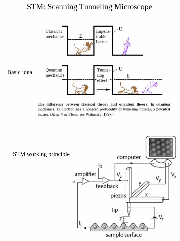
STM: Scanning Tunneling Microscope Basic idea STM working principle
Transcript of STM: Scanning Tunneling Microscope · approximately half the probing wavelength. For optical...
STM: Scanning Tunneling Microscope
Basic idea
STM working principle
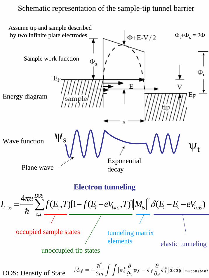
Schematic representation of the sample-tip tunnel barrier
ψs
Energy diagram
Electron tunneling2
,
4 ( , )[1 ( , )] ( )DOS
t s s t bias ts t s biast s
eI f E T f E eV T M E E eVπ δ→ = − + − −∑
occupied sample states
unoccupied tip states
tunneling matrixelements elastic tunneling
DOS: Density of State
Assume tip and sample describedby two infinite plate electrodes
Sample work function
ψtWave function
Plane waveExponential decay
Φs
Φt
Φt+Φs = 2Φ

2
,
4 [ ( , ) ( , )] ( )
t s s t
t s bias ts t s biast s
I I Ie f E T f E eV T M E E eVπ δ
→ →= − =
− + − −∑
( ) , ( )t st s
dE E dE Eρ ρ→ →∑ ∑∫ ∫
[ ] 24 ( ) ( ) ( ) ( ) ( )F F S F t FeI f E f E eV E eV E M dπ ε ε ρ ε ρ ε ε ε∞
−∞
= + − + + + + +∫sample and tip DOS
For small kT, f(E) step function
2
0
4 ( ) ( ) ( )eV
S F t FeI E eV E M dπ ρ ε ρ ε ε ε= + + +∫
And for small Vbias
224 ( ) ( )S F T F
eI V E E Mπ ρ ρ=
224 ( ) ( )S F T F
dI e E eV E MdV
π ρ ρ= +
Electron tunneling
Moving to the continuous
The tunneling current is a function of the tip and sample density of state close to the Fermi level

( ) ( ) ( )20 ,
t t
z m eVz e κψ ψ κ− Φ −= =
( ) ( ) ( )0s
d zs z e κψ ψ − −=
Assuming the electron wave functions for tip and sample described by plane waves, the quantum mechanics predicts an exponential decay in the vacuum gap following
2( ) ( ) zS F T FI V E E e κρ ρ −∝
STM vertical resolution
For small T and V
Φ in [eV] d in [Å]
1.025 1 100dI eI
ΦΔΔ≈ − ≈
1.025( ) ( ) dS F T FI V E E eρ ρ − Φ∝
N.B.: if the tip (sample) is an insulator -> ρt(EF) (ρs(EF)) = 0 implying I = 0
The STM is useless in this case
Typically Φ = 5 eV
Easy to measure ΔI/I = 0.1 -> Δd = Φ-0.5 ΔI/I = 0.05 Å
Atomic step Δd = 2 Å
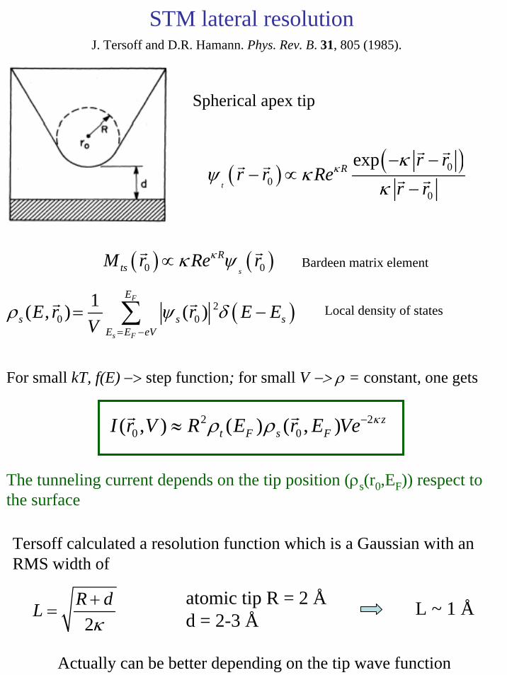
J. Tersoff and D.R. Hamann. Phys. Rev. B. 31, 805 (1985).
For small kT, f(E) −> step function; for small V −> ρ = constant, one gets
( ) ( )00
0
expt
R r rr r Re
r rκ κ
ψ κκ− −
− ∝−
( )20 0
1( , ) ( )F
s F
E
s s sE E eV
E r r E EV
ρ ψ δ= −
= −∑
( ) ( )0 0s
RtsM r Re rκκ ψ∝ Bardeen matrix element
Local density of states
Spherical apex tip
STM lateral resolution
2 20 0( , ) ( ) ( , ) z
t F s FI r V R E r E Ve κρ ρ −≈
The tunneling current depends on the tip position (ρs(r0,EF)) respect to the surface
Tersoff calculated a resolution function which is a Gaussian with an RMS width of
2R dLκ+
=atomic tip R = 2 Åd = 2-3 Å L ~ 1 Å
Actually can be better depending on the tip wave function
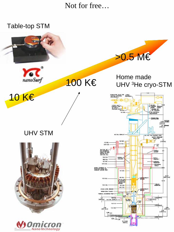
>0.5 M€
10 K€
Table-top STM
Home made UHV 3He cryo-STM100 K€
UHV STM
Not for free…
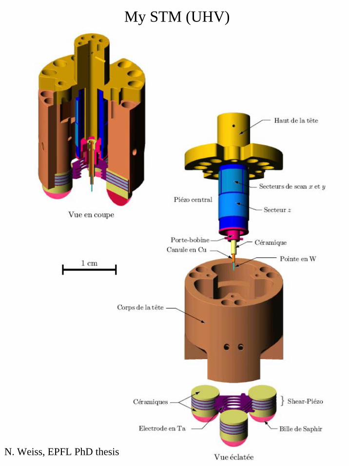
My STM (UHV)
N. Weiss, EPFL PhD thesis
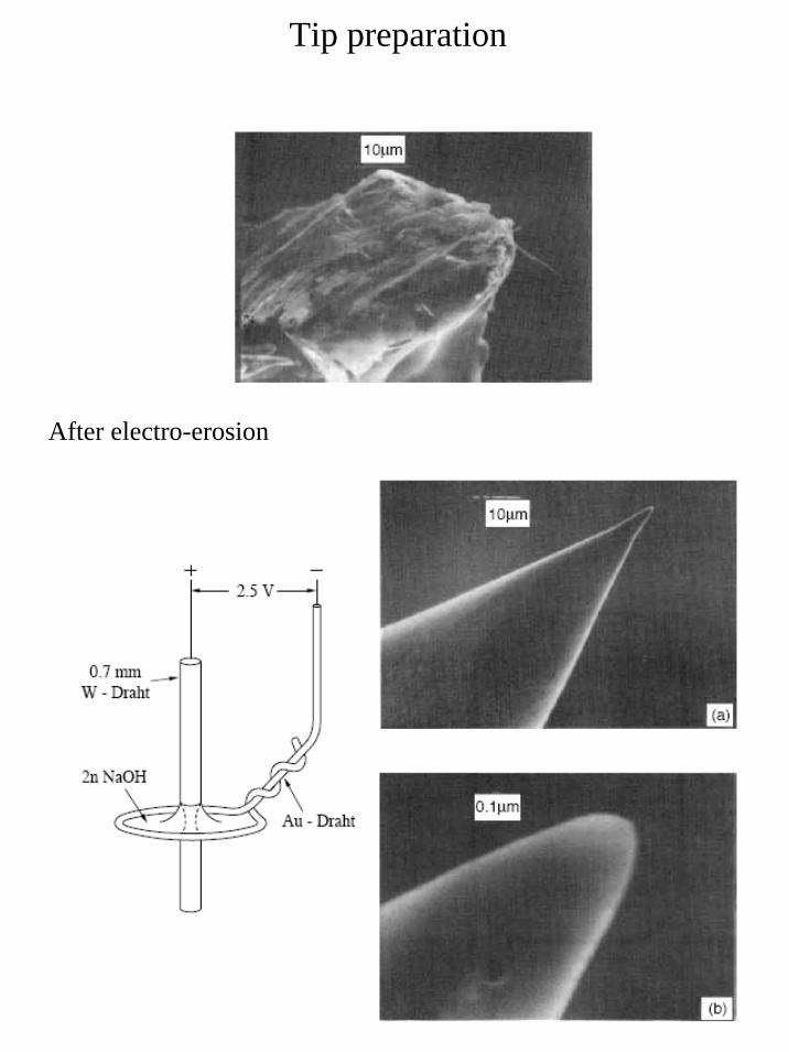
Tip preparation
After electro-erosion
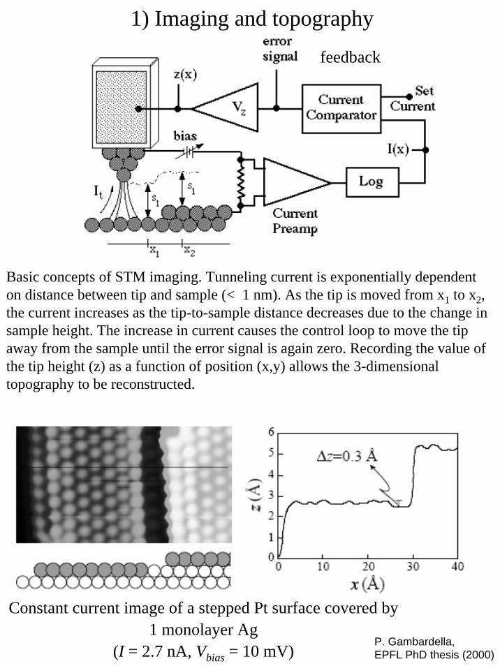
1) Imaging and topography
Constant current image of a stepped Pt surface covered by 1 monolayer Ag
(I = 2.7 nA, Vbias = 10 mV)P. Gambardella, EPFL PhD thesis (2000)
Basic concepts of STM imaging. Tunneling current is exponentially dependent on distance between tip and sample (< 1 nm). As the tip is moved from x1 to x2, the current increases as the tip-to-sample distance decreases due to the change in sample height. The increase in current causes the control loop to move the tip away from the sample until the error signal is again zero. Recording the value of the tip height (z) as a function of position (x,y) allows the 3-dimensional topography to be reconstructed.
feedback
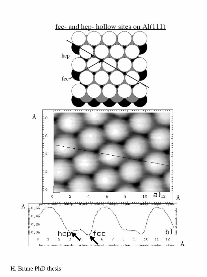
H. Brune PhD thesis
Å
Å
Å
Å

Warning !!!
1.025( ) ( ) dS F T FI V E E eρ ρ − Φ∝
Remember: the tunneling current is a measure of the Local Density of States (at the Fermi level) of tip and sample
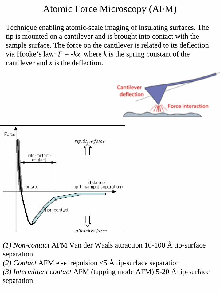
Technique enabling atomic-scale imaging of insulating surfaces. The tip is mounted on a cantilever and is brought into contact with the sample surface. The force on the cantilever is related to its deflection via Hooke’s law: F = -kx, where k is the spring constant of the cantilever and x is the deflection.
Atomic Force Microscopy (AFM)
(1) Non-contact AFM Van der Waals attraction 10-100 Å tip-surface separation(2) Contact AFM e--e- repulsion <5 Å tip-surface separation(3) Intermittent contact AFM (tapping mode AFM) 5-20 Å tip-surfaceseparation
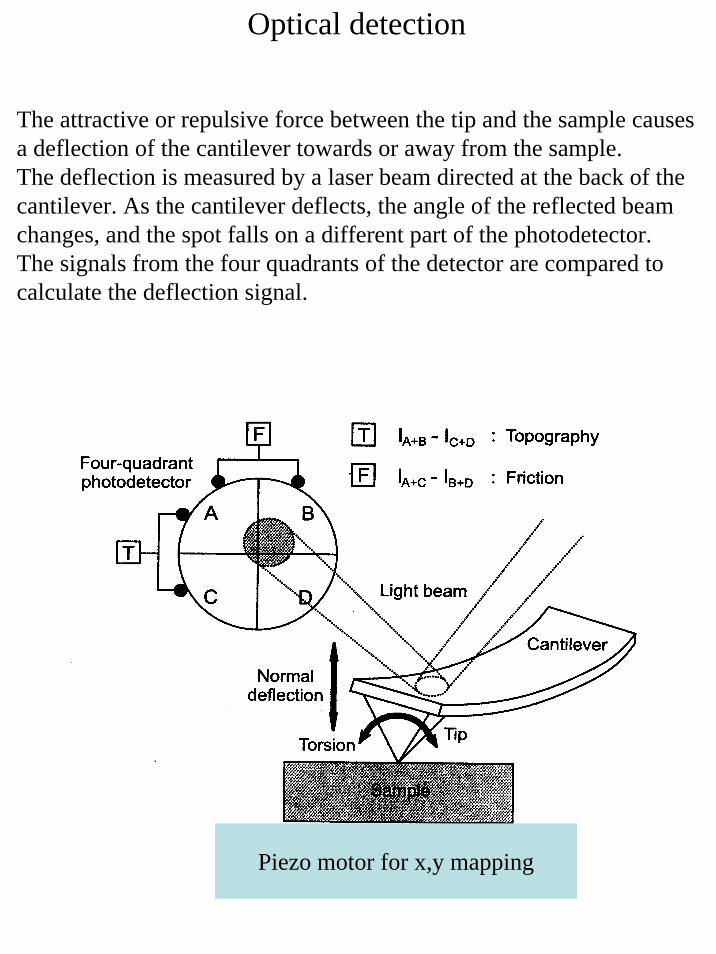
The attractive or repulsive force between the tip and the sample causes a deflection of the cantilever towards or away from the sample.The deflection is measured by a laser beam directed at the back of the cantilever. As the cantilever deflects, the angle of the reflected beam changes, and the spot falls on a different part of the photodetector.The signals from the four quadrants of the detector are compared to calculate the deflection signal.
Piezo motor for x,y mapping
Optical detection

(1) In contact mode:F(x) = -k × x Hooke's LawSpring constant of cantilever is less than surface, cantilever bends. Typical atom-atom k ~ 10 N·m-1, typical cantilever k 0.1-1 N·m-1
Total force on sample 10-6 to 10-8 NIf spring constant of cantilever is greater than surface, surface deformed.This mode can be used for very high resolution imaging, such as atomic resolution
(3) In intermittent contact (tapping) mode:Similar to non-contact AFM using vibrating cantilever except at one extent tip "taps" into contact modeUseful for soft surfaces - less prone to external vibration/noise than non-contactLess destructive than contact AFM and can image rougher samples
DNA acquired in tapping mode

(2) In non-contact mode:Very small force on surface (~ 10-12 N)- tip-surface distance 10-100 Å- best for soft or elastic surfaces- least contamination- least destructive- long tip lifeIn non-contact mode the cantilever oscillates close to the sample surface, but without making contact with the surface : AC drivenoscillating cantilever (100-1000 Hz frequency, 10-100 Å amplitude)- resonant frequency ν =1/(2 π) sqrt(k/m)- k varies with external force gradient (dF(x)/dx) so frequency changes with external force- electronics adjust tip-surface distance to keep resonant frequencyconstant -> constant tip forceContact and non-contact show similar topography except for soft/deformable materials
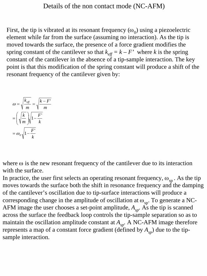
First, the tip is vibrated at its resonant frequency (ω0) using a piezoelectric element while far from the surface (assuming no interaction). As the tip is moved towards the surface, the presence of a force gradient modifies the spring constant of the cantilever so that keff = k – F’ where k is the spring constant of the cantilever in the absence of a tip-sample interaction. The key point is that this modification of the spring constant will produce a shift of the resonant frequency of the cantilever given by:
kF
kF
mk
mFk
mkeff
'1
'1
'
0 −=
−⎟⎟⎠
⎞⎜⎜⎝
⎛=
−==
ω
ω
where ω is the new resonant frequency of the cantilever due to its interaction with the surface.In practice, the user first selects an operating resonant frequency, ωsp . As the tip moves towards the surface both the shift in resonance frequency and the damping of the cantilever’s oscillation due to tip-surface interactions will produce a corresponding change in the amplitude of oscillation at ωsp. To generate a NC-AFM image the user chooses a set-point amplitude, Asp. As the tip is scanned across the surface the feedback loop controls the tip-sample separation so as to maintain the oscillation amplitude constant at Asp. A NC-AFM image therefore represents a map of a constant force gradient (defined by Asp) due to the tip-sample interaction.
Details of the non contact mode (NC-AFM)

The method in theory:
Contact mode topography (left) and non contact mode image (right) of a two-phase block copolymer.
The result in image:

5 μm
Mechanical characteristics of the AFM cantilever
SEM images Dimensions

Magnetic Force Microscopy (MFM)
Topography
Magnetism
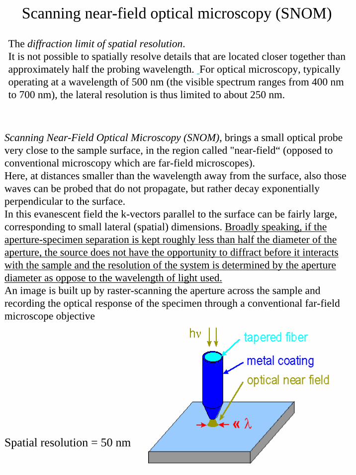
Scanning near-field optical microscopy (SNOM)
Spatial resolution = 50 nm
The diffraction limit of spatial resolution. It is not possible to spatially resolve details that are located closer together than approximately half the probing wavelength. For optical microscopy, typically operating at a wavelength of 500 nm (the visible spectrum ranges from 400 nm to 700 nm), the lateral resolution is thus limited to about 250 nm.
Scanning Near-Field Optical Microscopy (SNOM), brings a small optical probe very close to the sample surface, in the region called "near-field“ (opposed to conventional microscopy which are far-field microscopes). Here, at distances smaller than the wavelength away from the surface, also those waves can be probed that do not propagate, but rather decay exponentially perpendicular to the surface. In this evanescent field the k-vectors parallel to the surface can be fairly large, corresponding to small lateral (spatial) dimensions. Broadly speaking, if the aperture-specimen separation is kept roughly less than half the diameter of the aperture, the source does not have the opportunity to diffract before it interacts with the sample and the resolution of the system is determined by the aperture diameter as oppose to the wavelength of light used.An image is built up by raster-scanning the aperture across the sample and recording the optical response of the specimen through a conventional far-field microscope objective

SNOM is a technique based on the STM. In a SNOM experiment, a fiber tip is scanned in close proximity across a sample, and optical information like reflectivity, fluorescence, luminescence or polarization can be derived with sub-wavelength resolution. In addition, topographical information can usually be obtained, since a local interaction (e.g. the lateral force between tip and sample surface) is used for control of the tip-sample distance, in a similar way as in an atomic force microscope (AFM)
A typical instrument consists illumination (laser, fiber coupler) and collection optics (objectives, filters, photomultipliers for moderate light levels or photon counters of very low intensities), fiber tip holder with shear force feedback (oscillator and lock-in amplifier), an approach scheme (mechanical or motorized), and a scanner (piezo tubes or stacks, it is often advantageous to scan the sample rather than the probe). Digital data acquisition and anti-vibration damping (optical tables, actively or passively dampened) completes the equipment. The microscope shown here sits on a conventional (inverted) light microscope, which allows to localize the sample with low resolution prior to SNOM operation.
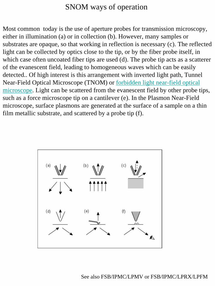
Most common today is the use of aperture probes for transmission microscopy,either in illumination (a) or in collection (b). However, many samples or substrates are opaque, so that working in reflection is necessary (c). The reflected light can be collected by optics close to the tip, or by the fiber probe itself, in which case often uncoated fiber tips are used (d). The probe tip acts as a scattererof the evanescent field, leading to homogeneous waves which can be easily detected.. Of high interest is this arrangement with inverted light path, Tunnel Near-Field Optical Microscope (TNOM) or forbidden light near-field optical microscope. Light can be scattered from the evanescent field by other probe tips, such as a force microscope tip on a cantilever (e). In the Plasmon Near-Field microscope, surface plasmons are generated at the surface of a sample on a thin film metallic substrate, and scattered by a probe tip (f).
See also FSB/IPMC/LPMV or FSB/IPMC/LPRX/LPFM
SNOM ways of operation