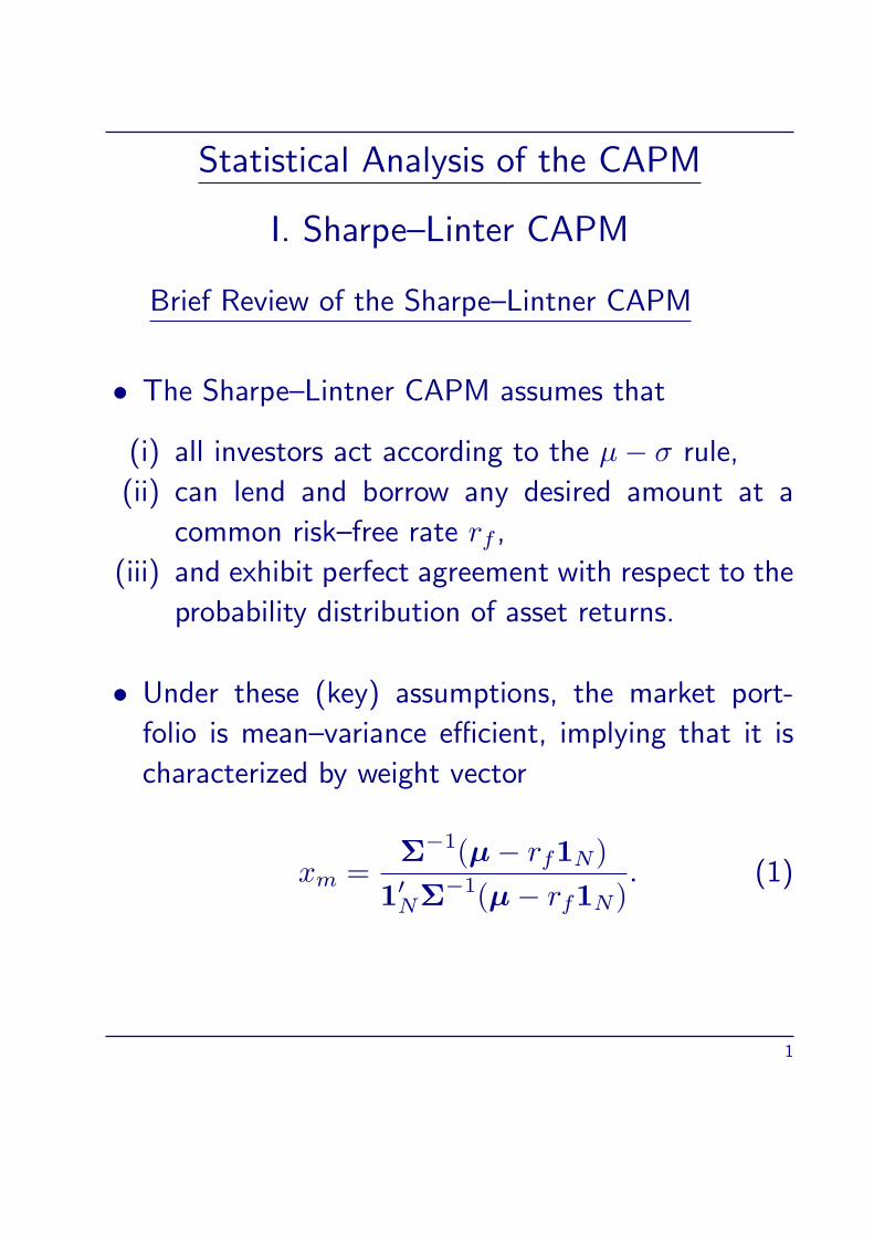
Statistical Analysis of the CAPM

I. Sharpe–Linter CAPM

Brief Review of the Sharpe–Lintner CAPM

• The Sharpe–Lintner CAPM assumes that

(i) all investors act according to the µ− σ rule,

(ii) can lend and borrow any desired amount at a

common risk–free rate rf ,

(iii) and exhibit perfect agreement with respect to the

probability distribution of asset returns.

• Under these (key) assumptions, the market port-

folio is mean–variance efficient, implying that it is

characterized by weight vector

xm =Σ−1(µ− rf1N)

1′NΣ−1(µ− rf1N)

. (1)

1

• The central equation of the Sharpe–Lintner CAPM

is a direct consequence of (1) and is given by

µi − rf = βi(µm − rf), i = 1, . . . , N, (2)

where

– rf is the risk–free rate,

– µm is the expected return of the market portfolio,

and

– βi = COV (Ri, Rm)/σ2m, where

– Ri is the return of asset i and Rm is the return

of the market portfolio.

• Equation (2) states that there is a linear relation

between the excess return of asset i (over the

risk–free) rate and the excess return of the market

portfolio, with zero intercept.

• Equation (2) also implies efficiency.

2

Framework for Estimation and Testing

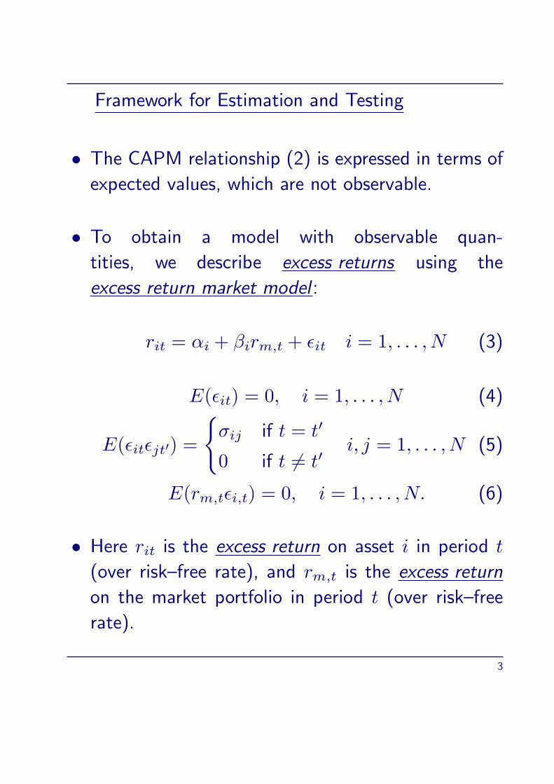
• The CAPM relationship (2) is expressed in terms of

expected values, which are not observable.

• To obtain a model with observable quan-

tities, we describe excess returns using the

excess return market model :

rit = αi + βirm,t + ϵit i = 1, . . . , N (3)

E(ϵit) = 0, i = 1, . . . , N (4)

E(ϵitϵjt′) =

σij if t = t′

0 if t = t′i, j = 1, . . . , N (5)

E(rm,tϵi,t) = 0, i = 1, . . . , N. (6)

• Here rit is the excess return on asset i in period t

(over risk–free rate), and rm,t is the excess return

on the market portfolio in period t (over risk–free

rate).

3

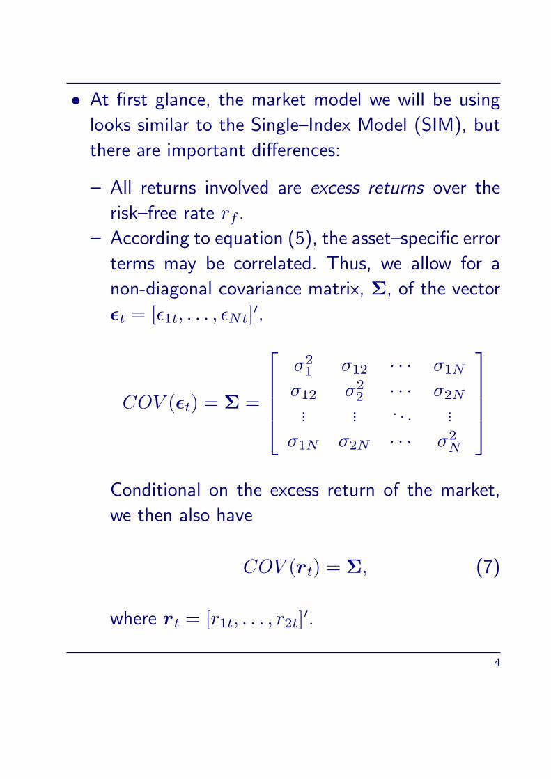
• At first glance, the market model we will be using

looks similar to the Single–Index Model (SIM), but

there are important differences:

– All returns involved are excess returns over the

risk–free rate rf .

– According to equation (5), the asset–specific error

terms may be correlated. Thus, we allow for a

non-diagonal covariance matrix, Σ, of the vector

ϵt = [ϵ1t, . . . , ϵNt]′,

COV (ϵt) = Σ =

σ21 σ12 · · · σ1N

σ12 σ22 · · · σ2N

... ... . . . ...

σ1N σ2N · · · σ2N

Conditional on the excess return of the market,

we then also have

COV (rt) = Σ, (7)

where rt = [r1t, . . . , r2t]′.

4

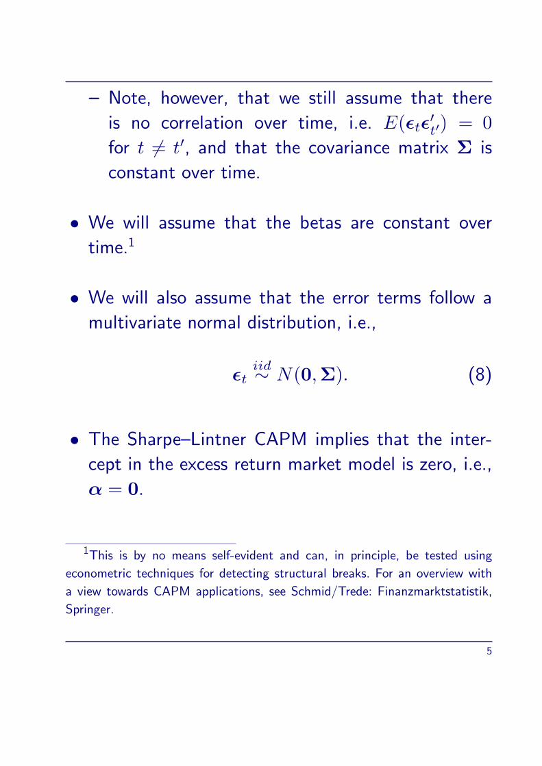
– Note, however, that we still assume that there

is no correlation over time, i.e. E(ϵtϵ′t′) = 0

for t = t′, and that the covariance matrix Σ is

constant over time.

• We will assume that the betas are constant over

time.1

• We will also assume that the error terms follow a

multivariate normal distribution, i.e.,

ϵtiid∼ N(0,Σ). (8)

• The Sharpe–Lintner CAPM implies that the inter-

cept in the excess return market model is zero, i.e.,

α = 0.

1This is by no means self-evident and can, in principle, be tested using

econometric techniques for detecting structural breaks. For an overview with

a view towards CAPM applications, see Schmid/Trede: Finanzmarktstatistik,

Springer.

5

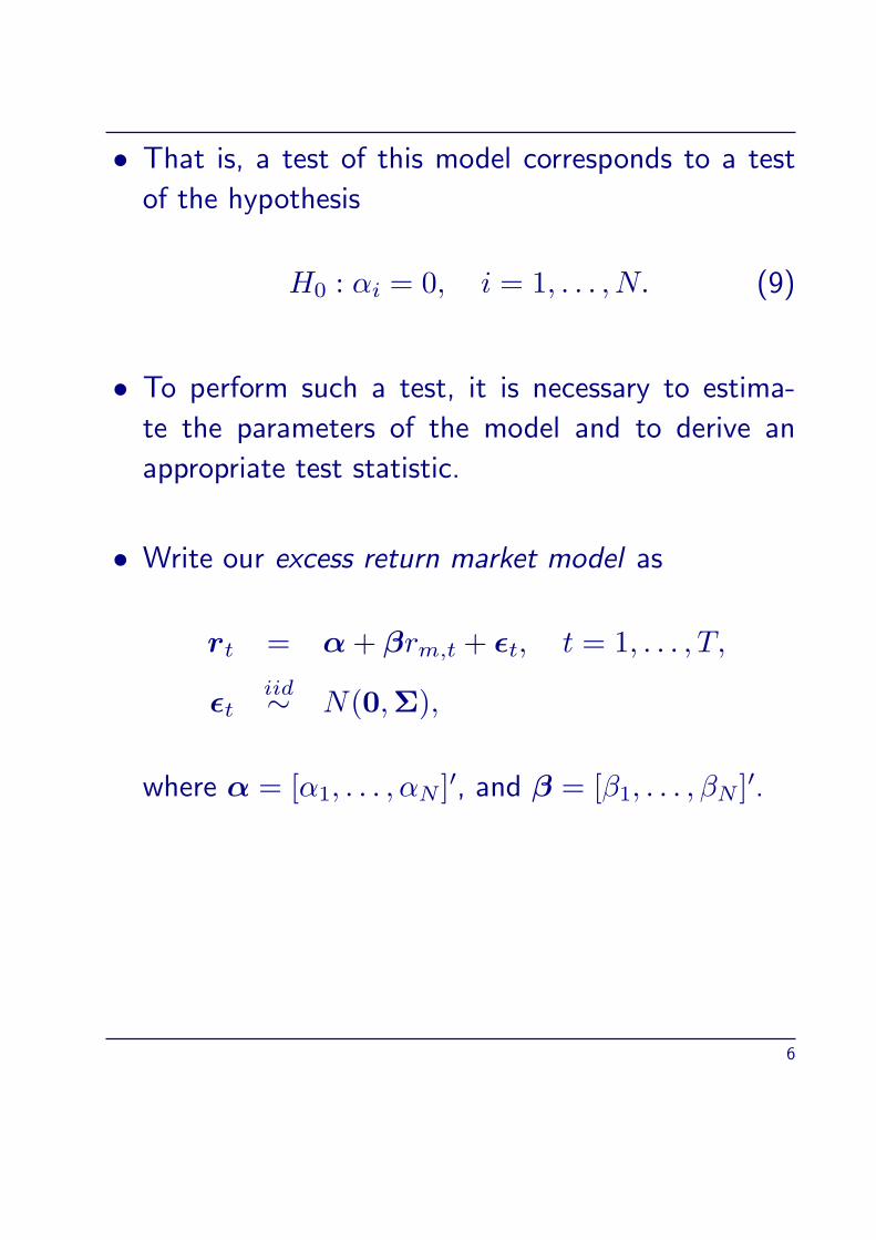
• That is, a test of this model corresponds to a test

of the hypothesis

H0 : αi = 0, i = 1, . . . , N. (9)

• To perform such a test, it is necessary to estima-

te the parameters of the model and to derive an

appropriate test statistic.

• Write our excess return market model as

rt = α+ βrm,t + ϵt, t = 1, . . . , T,

ϵtiid∼ N(0,Σ),

where α = [α1, . . . , αN ]′, and β = [β1, . . . , βN ]′.

6

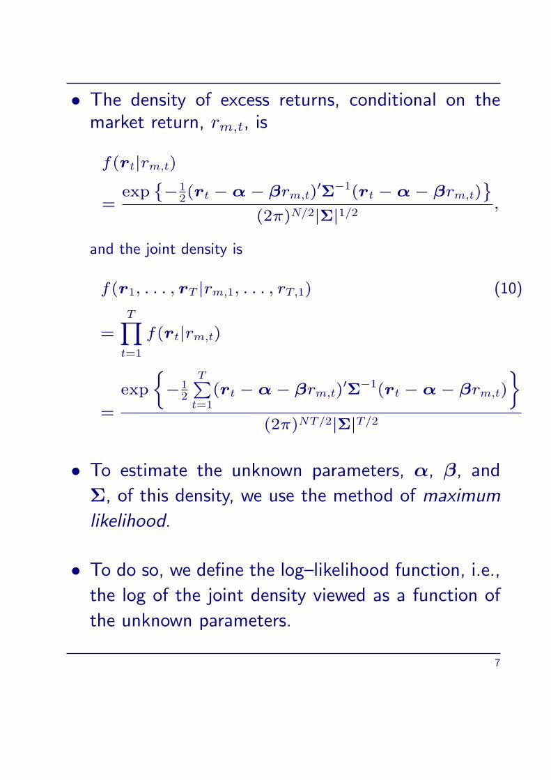
• The density of excess returns, conditional on themarket return, rm,t, is

f(rt|rm,t)

=exp

−1

2(rt − α − βrm,t)′Σ−1(rt − α − βrm,t)

(2π)N/2|Σ|1/2

,

and the joint density is

f(r1, . . . , rT |rm,1, . . . , rT,1) (10)

=T∏

t=1

f(rt|rm,t)

=

exp

−1

2

T∑t=1

(rt − α − βrm,t)′Σ−1(rt − α − βrm,t)

(2π)NT/2|Σ|T/2

• To estimate the unknown parameters, α, β, and

Σ, of this density, we use the method of maximum

likelihood.

• To do so, we define the log–likelihood function, i.e.,

the log of the joint density viewed as a function of

the unknown parameters.

7

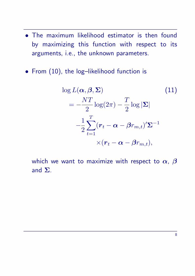
• The maximum likelihood estimator is then found

by maximizing this function with respect to its

arguments, i.e., the unknown parameters.

• From (10), the log–likelihood function is

logL(α,β,Σ) (11)

= −NT

2log(2π)− T

2log |Σ|

−1

2

T∑t=1

(rt −α− βrm,t)′Σ−1

×(rt −α− βrm,t),

which we want to maximize with respect to α, β

and Σ.

8

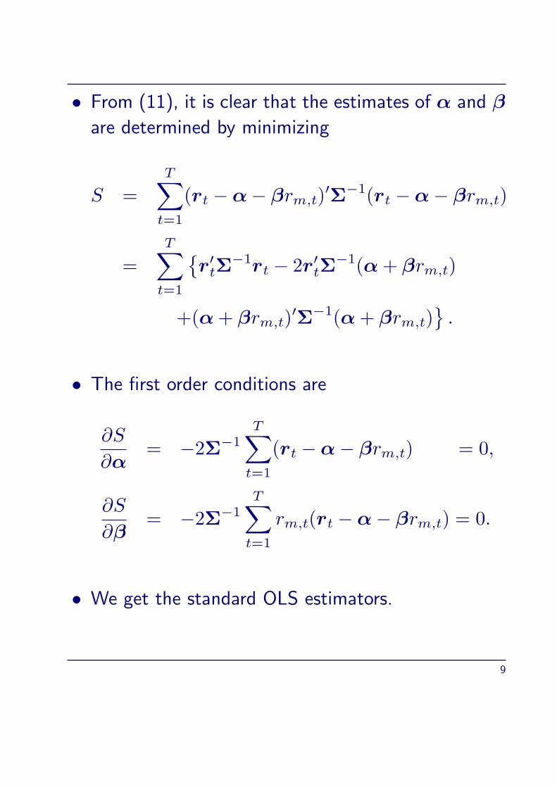
• From (11), it is clear that the estimates of α and β

are determined by minimizing

S =

T∑t=1

(rt −α− βrm,t)′Σ−1(rt −α− βrm,t)

=

T∑t=1

r′tΣ

−1rt − 2r′tΣ−1(α+ βrm,t)

+(α+ βrm,t)′Σ−1(α+ βrm,t)

.

• The first order conditions are

∂S

∂α= −2Σ−1

T∑t=1

(rt −α− βrm,t) = 0,

∂S

∂β= −2Σ−1

T∑t=1

rm,t(rt −α− βrm,t) = 0.

• We get the standard OLS estimators.

9

• That is,

α = r − βrm

and

β =

∑Tt=1(rt − r)(rm,t − rm)∑T

t=1(rm,t − rm)2

=

∑Tt=1(rt − r)(rm,t − rm)

T σ2m

=

∑Tt=1(rm,t − rm)rt

T σ2m

where

r =1

T

T∑t=1

rt, rm =1

T

T∑t=1

rm,t,

σ2m =

1

T

T∑t=1

(rm,t − rm)2.

10

• To find the MLE of Σ, we make use of the following

differentiation rules:

(i) Let X and A be n× n matrices, so that

tr(XA) =n∑

i=1

n∑j=1

xijaji. (12)

For symmetric X (xij = xji), we therefore have

∂tr(XA)

∂xij=

aii i = j

aij + aji i = j.(13)

Hence

∂tr(XA)

∂X= A+A′ − diag(A),

and∂tr(XA)

∂X= 2A− diag(A), (14)

if A is also symmetric.

11

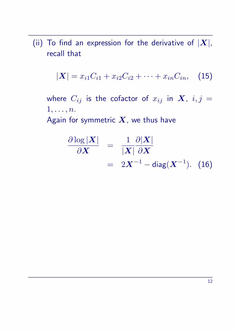
(ii) To find an expression for the derivative of |X|,recall that

|X| = xi1Ci1 + xi2Ci2 + · · ·+ xinCin, (15)

where Cij is the cofactor of xij in X, i, j =

1, . . . , n.

Again for symmetric X, we thus have

∂ log |X|∂X

=1

|X|∂|X|∂X

= 2X−1 − diag(X−1). (16)

12

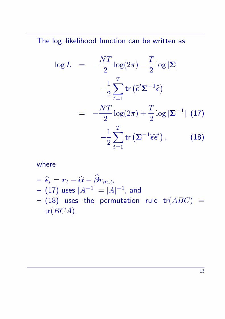
The log–likelihood function can be written as

logL = −NT

2log(2π)− T

2log |Σ|

−1

2

T∑t=1

tr(ϵ′Σ−1ϵ

)= −NT

2log(2π) +

T

2log |Σ−1| (17)

−1

2

T∑t=1

tr(Σ−1ϵϵ′

), (18)

where

– ϵt = rt − α− βrm,t,

– (17) uses |A−1| = |A|−1, and

– (18) uses the permutation rule tr(ABC) =

tr(BCA).

13

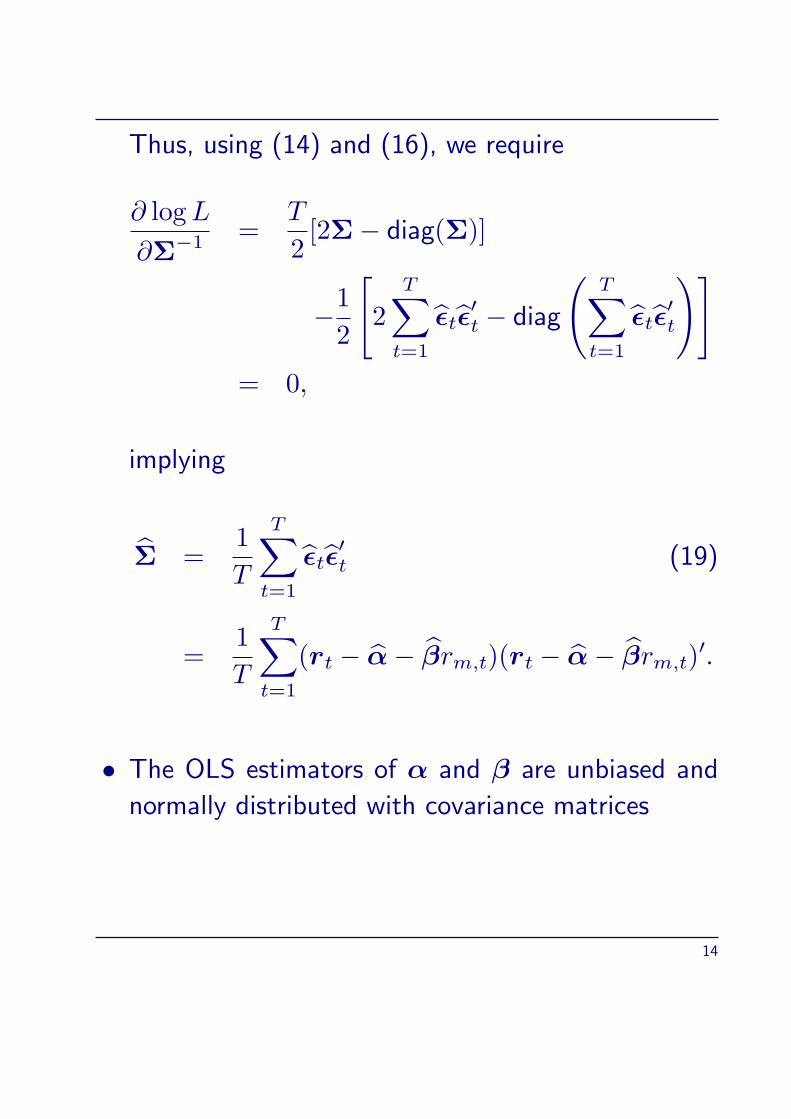
Thus, using (14) and (16), we require

∂ logL

∂Σ−1 =T

2[2Σ− diag(Σ)]

−1

2

[2

T∑t=1

ϵtϵ′t − diag

(T∑

t=1

ϵtϵ′t

)]= 0,

implying

Σ =1

T

T∑t=1

ϵtϵ′t (19)

=1

T

T∑t=1

(rt − α− βrm,t)(rt − α− βrm,t)′.

• The OLS estimators of α and β are unbiased and

normally distributed with covariance matrices

14

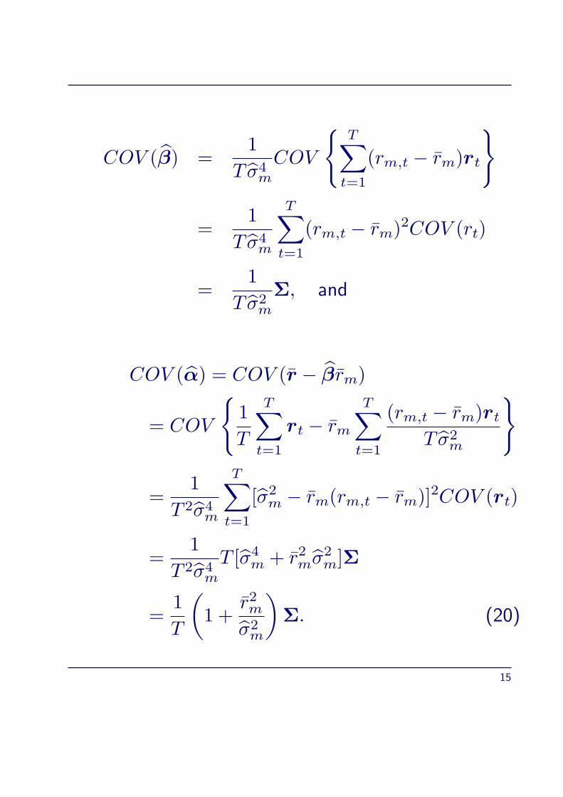
COV (β) =1

T σ4m

COV

T∑

t=1

(rm,t − rm)rt

=1

T σ4m

T∑t=1

(rm,t − rm)2COV (rt)

=1

T σ2m

Σ, and

COV (α) = COV (r − βrm)

= COV

1

T

T∑t=1

rt − rm

T∑t=1

(rm,t − rm)rtT σ2

m

=1

T 2σ4m

T∑t=1

[σ2m − rm(rm,t − rm)]2COV (rt)

=1

T 2σ4m

T [σ4m + r2mσ2

m]Σ

=1

T

(1 +

r2mσ2m

)Σ. (20)

15

• It can be shown that T Σ has a Wishart distribution,

WN(T − 2,Σ), which is a matrix generalization of

the χ2 distribution.2

Moreover, Σ is independent of both α and β.

2See, for example, Zellner (1971).

16

Testing for mean–variance efficiency (α = 0)

• We discuss two tests of the null hypothesis α = 0,

in historical order.

• The first is a likelihood ratio (LR) test relying on

asymptotic arguments,

• The second is an exact finite–sample F-test. Sub-

sequently, the relation between the tests will be

considered.

Likelihood Ratio (LR) Test

• To conduct the likelihood ratio test, we first com-

pute the Maximum Likelihood Estimator under the

null hypothesis that α = 0, which is a regressi-

on through the origin. Denote the corresponding

estimators by β0 and Σ0. They are given by

β0 =

∑Tt=1 rtrm,t∑Tt=1 r

2m,t

, (21)

17

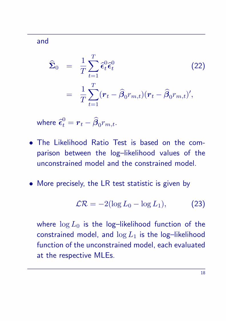
and

Σ0 =1

T

T∑t=1

ϵ0t ϵ0t (22)

=1

T

T∑t=1

(rt − β0rm,t)(rt − β0rm,t)′,

where ϵ0t = rt − β0rm,t.

• The Likelihood Ratio Test is based on the com-

parison between the log–likelihood values of the

unconstrained model and the constrained model.

• More precisely, the LR test statistic is given by

LR = −2(logL0 − logL1), (23)

where logL0 is the log–likelihood function of the

constrained model, and logL1 is the log–likelihood

function of the unconstrained model, each evaluated

at the respective MLEs.

18

• The asymptotic distribution of LR defined in (23)

is χ2 with degrees of freedom equal to the num-

ber of parameter restrictions implied by the null

hypothesis.

• In our situation, this corresponds to N degrees of

freedom (N is the number of assets), because the

CAPM implies that αi = 0 for i = 1, . . . , N .

19

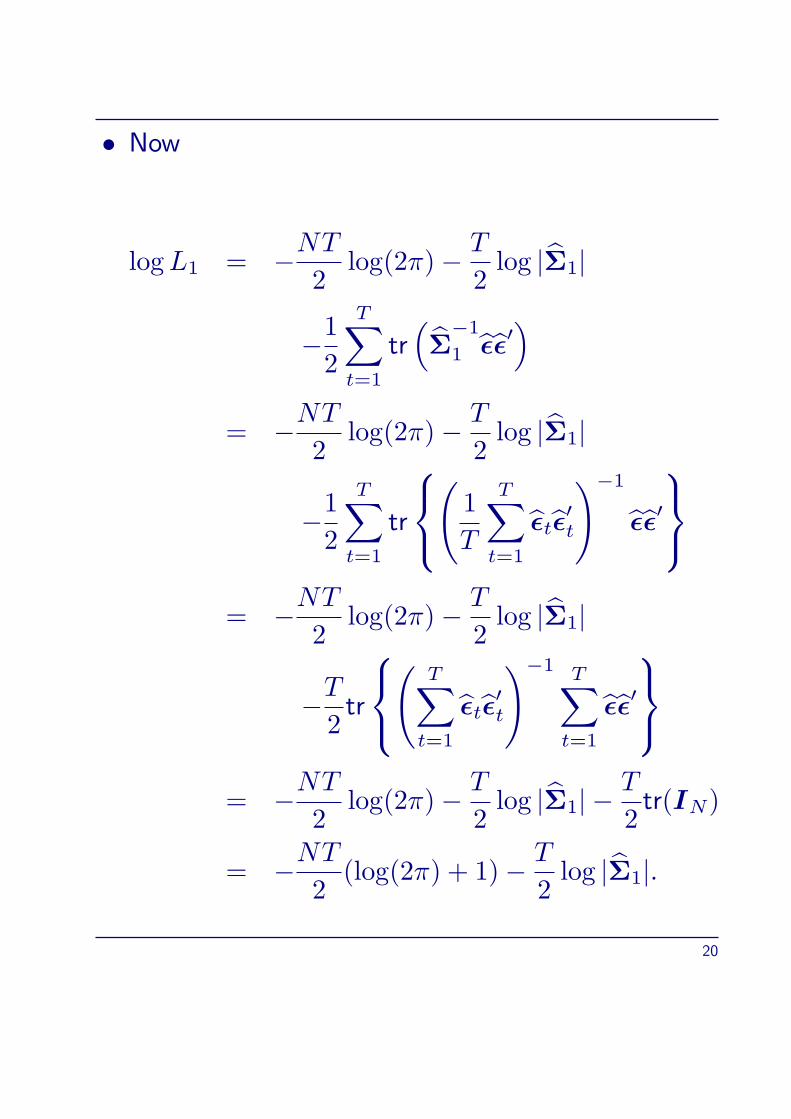
• Now

logL1 = −NT

2log(2π)− T

2log |Σ1|

−1

2

T∑t=1

tr(Σ

−1

1 ϵϵ′)

= −NT

2log(2π)− T

2log |Σ1|

−1

2

T∑t=1

tr

(1

T

T∑t=1

ϵtϵ′t

)−1

ϵϵ′

= −NT

2log(2π)− T

2log |Σ1|

−T

2tr

(

T∑t=1

ϵtϵ′t

)−1 T∑t=1

ϵϵ′

= −NT

2log(2π)− T

2log |Σ1| −

T

2tr(IN)

= −NT

2(log(2π) + 1)− T

2log |Σ1|.

20

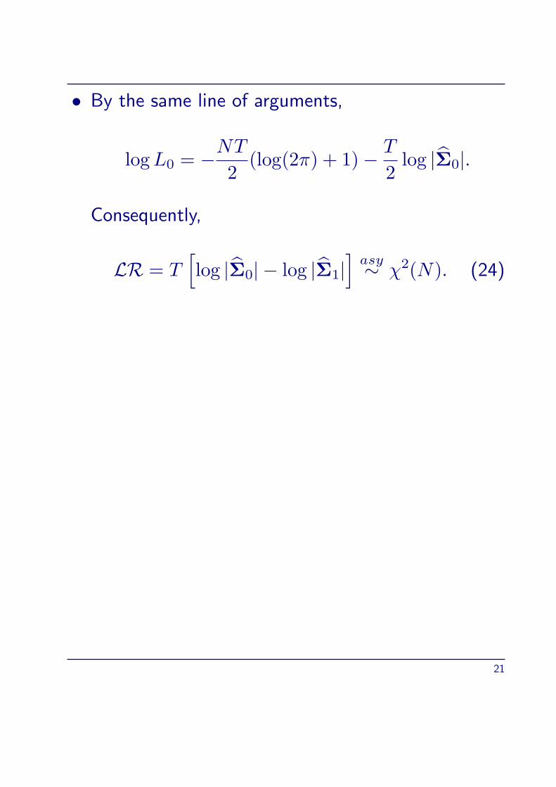
• By the same line of arguments,

logL0 = −NT

2(log(2π) + 1)− T

2log |Σ0|.

Consequently,

LR = T[log |Σ0| − log |Σ1|

]asy∼ χ2(N). (24)

21

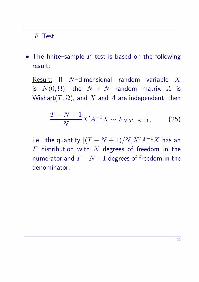
F Test

• The finite–sample F test is based on the following

result:

Result: If N–dimensional random variable X

is N(0,Ω), the N × N random matrix A is

Wishart(T,Ω), and X and A are independent, then

T −N + 1

NX ′A−1X ∼ FN,T−N+1, (25)

i.e., the quantity [(T −N + 1)/N ]X ′A−1X has an

F distribution with N degrees of freedom in the

numerator and T −N +1 degrees of freedom in the

denominator.

22

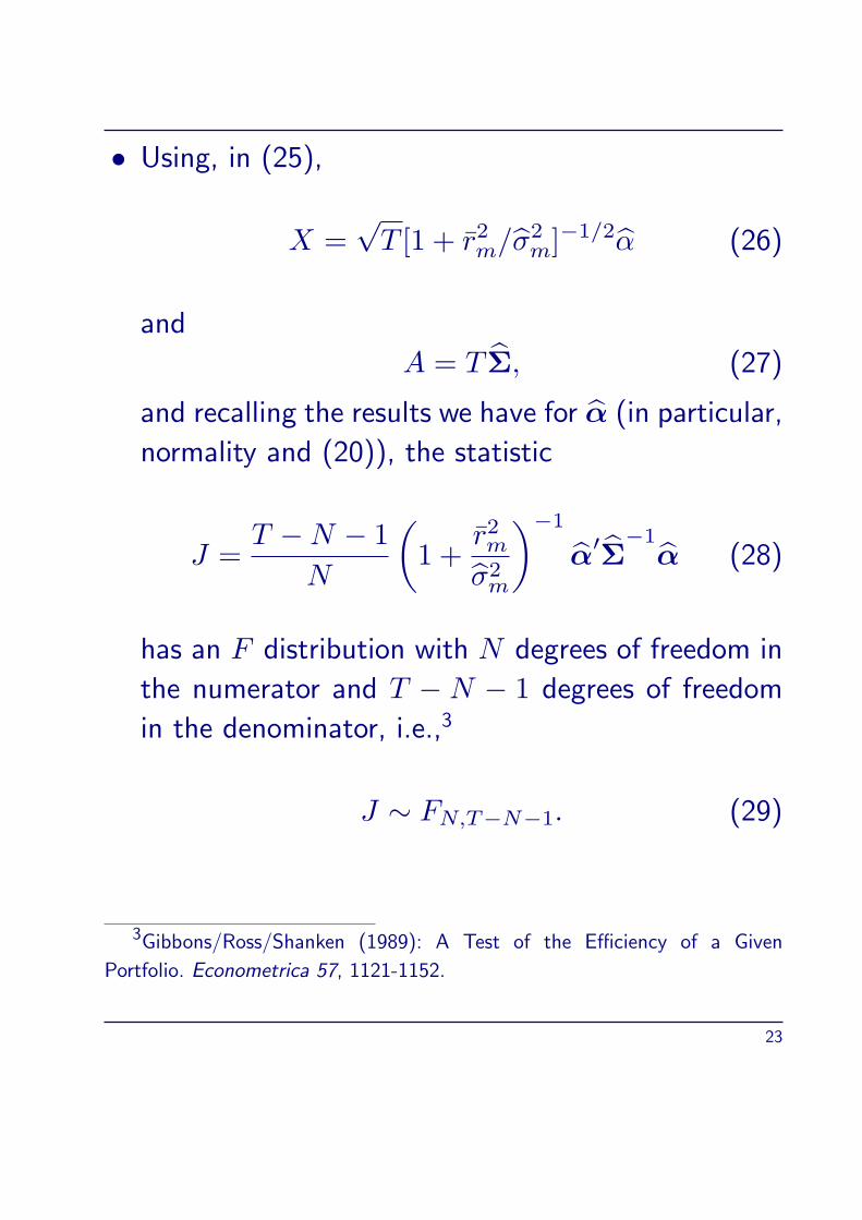
• Using, in (25),

X =√T [1 + r2m/σ2

m]−1/2α (26)

and

A = T Σ, (27)

and recalling the results we have for α (in particular,

normality and (20)), the statistic

J =T −N − 1

N

(1 +

r2mσ2m

)−1

α′Σ−1

α (28)

has an F distribution with N degrees of freedom in

the numerator and T − N − 1 degrees of freedom

in the denominator, i.e.,3

J ∼ FN,T−N−1. (29)

3Gibbons/Ross/Shanken (1989): A Test of the Efficiency of a Given

Portfolio. Econometrica 57, 1121-1152.

23

Economic Interpretation of the CAPM F Test

• Apart from following a known finite–sample distri-

bution, the test statistic J defined in (28) also has

economic interpretation.

• Recall that the key testable implication of the CAPM

is that the market portfolio is a µ − σ efficient

portfolio.

• In the presence of a risk–free rate, this means that

the market portfolio is the tangency portfolio.

24

• It can be shown that4

J =

(T −N − 1

N

)θ⋆2 − θ2m

1 + θ2m, (30)

where θ⋆ is the Sharpe ratio of the ex post (i.e.,

using the sample mean vector and the sample co-

variance matrix) efficient portfolio formed from the

risky assets under study (including our market proxy)

and θm is the Sharpe ratio of the portfolio used as

a market proxy in our analysis.

• Equation (30) is particularly interesting because it

uncovers what we are actually testing: We test

whether our market proxy is so far away from the

ex post efficient portfolio that we are not willing to

believe that it is the population tangency portfolio,

where the distance is measured in terms of the

Sharpe Ratio.

4Gibbons/Ross/Shanken (1989): A Test of the Efficiency of a Given

Portfolio. Econometrica 57, 1121-1152.

25

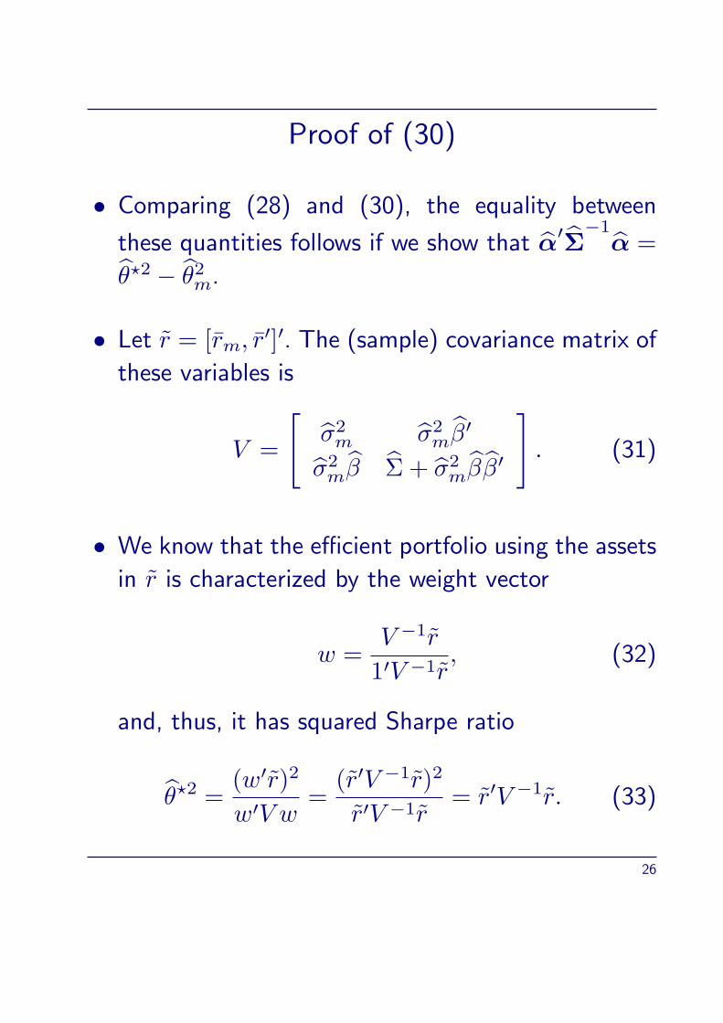
Proof of (30)

• Comparing (28) and (30), the equality between

these quantities follows if we show that α′Σ−1

α =

θ⋆2 − θ2m.

• Let r = [rm, r′]′. The (sample) covariance matrix of

these variables is

V =

[σ2m σ2

mβ′

σ2mβ Σ + σ2

mββ′

]. (31)

• We know that the efficient portfolio using the assets

in r is characterized by the weight vector

w =V −1r

1′V −1r, (32)

and, thus, it has squared Sharpe ratio

θ⋆2 =(w′r)2

w′V w=

(r′V −1r)2

r′V −1r= r′V −1r. (33)

26

• Next, it is easily checked that the inverse of (31) is

V −1 =

[σ−2m + β′Σ−1β −β′Σ−1

−Σ−1β Σ−1

](34)

• Using (34), we get by straightforward computation,

and using (33),

θ⋆2 = r′V −1r = [rm, r′]V −1[rm, r′]′

=r2mσ2m

+ (r − βrm)′Σ−1(r − βrm)

= θ2m + α′Σ−1α,

recalling that α = r − βrm.

27

Relation between F and LR tests

• The finite–sample F test can also be interpreted as

a likelihood ratio test.

• To see this, first note that for the unconstrained

MLE of β, denoted by β1,

β1 =

∑t(rm,t − rm)rt

T σ2m

=

∑t rm,trt − rm

∑t rt

T σ2m

=r2mσ2m

β0 −rmr

σ2m

=r2mσ2m

β0 −rmσ2m

(r − β1rm)− r2mσ2m

β1

=r2mσ2m

β0 −rmσ2m

α− r2mσ2m

β1.

Rearranging and using the basic identity

σ2m = r2m − r2m =

1

T

T∑t=1

r2m,t − r2m,

28

shows that

β0 = β1 +rm

σ2m + r2m

α. (35)

Inserting (35) into Σ0 (see equation (22)) and

noting that the normal equations (12) and (12)

imply

T∑t=1

(rt − α− β1rm,t)′(1− rmrm,t

r2m + σ2m

)α = 0,

we arrive at

Σ0 = Σ1 +

(σ2m

r2m + σ2m

)αα′. (36)

• The Sherman–Morrison formula for the determinant

is as follows: For nonsingular A and conformable

vectors u and v

|A+ uv′| = |A|(1 + v′A−1u). (37)

29

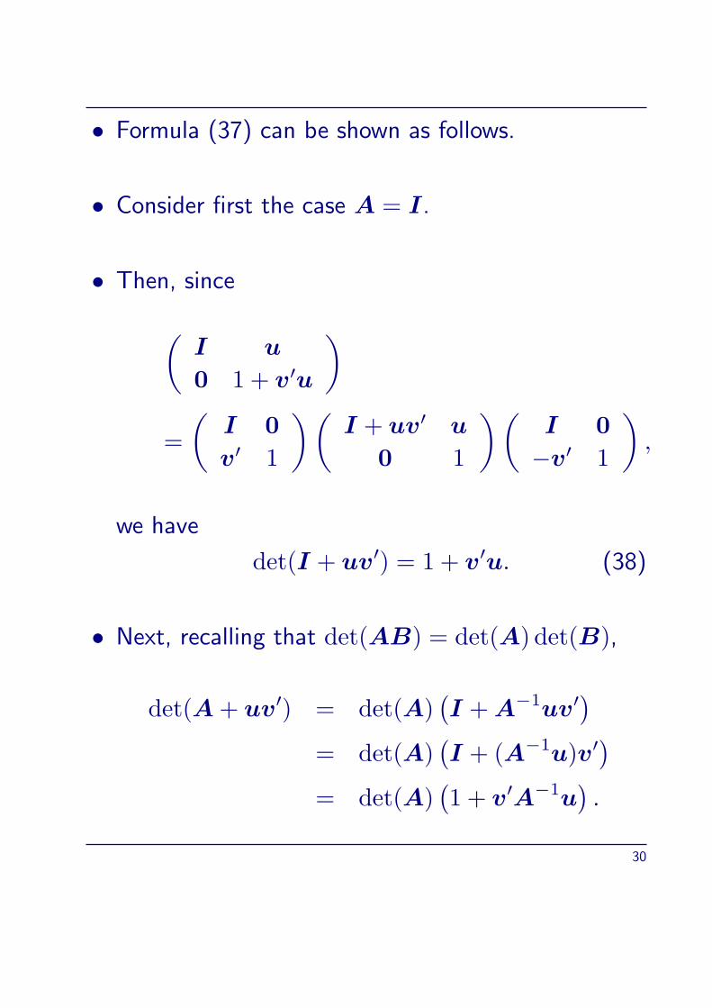
• Formula (37) can be shown as follows.

• Consider first the case A = I.

• Then, since

(I u

0 1 + v′u

)=

(I 0

v′ 1

)(I + uv′ u

0 1

)(I 0

−v′ 1

),

we have

det(I + uv′) = 1 + v′u. (38)

• Next, recalling that det(AB) = det(A) det(B),

det(A+ uv′) = det(A)(I +A−1uv′)

= det(A)(I + (A−1u)v′)

= det(A)(1 + v′A−1u

).

30

When this formula is applied to (36), we obtain

|Σ0| = |Σ1|[1 +

σ2m

r2m + σ2m

α′Σ−1

1 α

]Thus, (24) may be written as

LR = T log|Σ0||Σ1|

= T log

[1 +

σ2m

r2m + σ2m

α′Σ−1

1 α

]= T log

[N

T −N − 1J + 1

],

where J is the F–statistic given by (28), or, equi-

valently,

J =T −N − 1

N

[exp

LRT

− 1

], (39)

which, as (39) is a monotonic transformation of

LR, shows that J may also be interpreted as a

likelihood ratio test.

31

• As the F–test based on (28) is exact, it is, for

realistic sample sizes, clearly preferable compared

to the likelihood ratio test relying on asymptotic

arguments.

• However, for the zero–beta version, an exact test is

much more difficult to obtain, and it may be useful

to consider what is lost when relying on asymptotic

arguments.

32

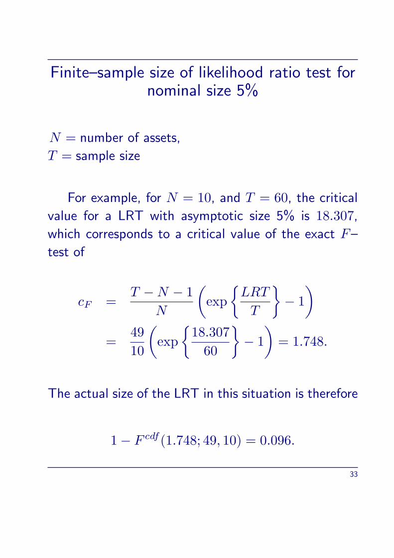
Finite–sample size of likelihood ratio test fornominal size 5%

N = number of assets,

T = sample size

For example, for N = 10, and T = 60, the critical

value for a LRT with asymptotic size 5% is 18.307,

which corresponds to a critical value of the exact F–

test of

cF =T −N − 1

N

(exp

LRT

T

− 1

)=

49

10

(exp

18.307

60

− 1

)= 1.748.

The actual size of the LRT in this situation is therefore

1− F cdf(1.748; 49, 10) = 0.096.

33

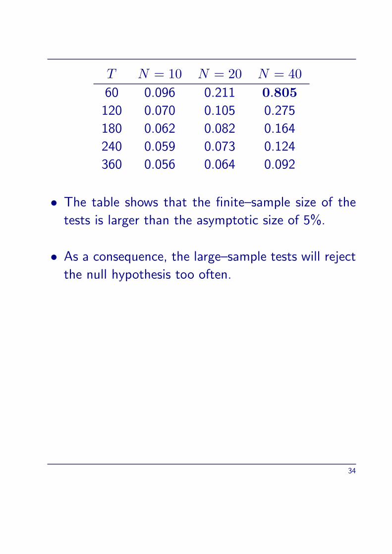
T N = 10 N = 20 N = 40

60 0.096 0.211 0.805

120 0.070 0.105 0.275

180 0.062 0.082 0.164

240 0.059 0.073 0.124

360 0.056 0.064 0.092

• The table shows that the finite–sample size of the

tests is larger than the asymptotic size of 5%.

• As a consequence, the large–sample tests will reject

the null hypothesis too often.

34

Roll’s Critique

• Roll (1977)5 emphasizes that tests of the CAPM

really only reject the mean–variance efficiency of

the market proxy we use in the test (recall equation

(30)).

• This implies that the CAPM is essentially untesta-

ble, because “the theory is not testable unless the

exact composition of the true market portfolio is

known and used in the tests. This implies that the

theory is not testable unless all individual assets are

included in the sample”.

5R. Roll (1977). A Critique of the Asset Pricing Theory’s Tests. Part I: On

Past and Potential Testability of the Theory. Journal of Financial Economics

4, 129-176.

35

• Roll argues that using a proxy for the market port-

folio is subject to two difficulties: “First, the proxy

itself might be mean–variance efficient even when

the true market portfolio is not. This is a real dan-

ger since every sample will display efficient portfolios

that satisfy perfectly all of the theory’s implicati-

ons. (...) On the other hand, the chosen proxy may

turn out to be inefficient; but obviously, this alone

implies nothing about the true market portfolio’s

efficiency”.

• Thus, what we essentially test is a joint hypothesis:

The CAPM and the hypothsis that the portfolio

used in the tests as the market proxy is the true

market portfolio.

• Clearly, it is extremely difficult to measure the “mar-

ket portfolio”, because this entity can, in principle,

include not just traded financial assets, but also

consumer durables, real estate, and human capital.

36

• On the other hand, often our interest is not to test

the CAPM (i.e., efficiency of the market portfolio)

but simply whether a specific portfolio is mean–

variance efficient within a given universe of assets.

37

References

• Campbell/Lo/MacKinlay (1997). The Econometrics

of Financial Markets. Princeton University Press:

Princeton.

• E. F. Fama and K. R. French (2004). The Capital

Asset Pricing Model: Theory and Evidence. Journal

of Economic Perspectives, 18, 25–46.

• F. Schmid and M. Trede (2006(?)). Finanzmarkt-

statistik, Springer, Kapitel 7.

• Zellner, A. (1971). Introduction to Bayesain Infe-

rence in Econometrics. New York: John Wiley &

Sons.

38