
Stationary performance evaluation measures in multi …skapodis/phdthesis_eng.pdf · 2009-09-09 ·...
141
University of Athens Department of Mathematics Section of Statistics and Operations Research Stationary performance evaluation measures in multi-dimensional Markov chains and applications in Queueing Theory Stella Kapodistria 0 1 2 ··· n - 2 n - 1 n ( n j )p n-j q j ×ν Athens 2009
Transcript of Stationary performance evaluation measures in multi …skapodis/phdthesis_eng.pdf · 2009-09-09 ·...
University of Athens
Department of Mathematics
Section of Statistics and Operations Research
Stationary performance evaluationmeasures in multi-dimensional Markov
chains and applications in Queueing Theory
Stella Kapodistria
0 1 2 · · · n ! 2 n ! 1 n!!""!!""
(nj)p
n!jqj!!
""
Athens
2009
Stationary performance evaluation measures inmulti-dimensional Markov chains and applications in
Queueing Theory
Stella Kapodistria
PhD Thesis
g
To Antonis, Vaso,
Espi
and Apostolos

With the completion of my PhD thesis, I would like to express my gratitude to
my supervisor A. Economou for his continuous guidance, his fruitful criticism, his
encouragement and support. His ideas, his intuition and his unique way of treating
mathematical problems has given me inspiration and guidance throughout my stud-
ies.
To continue, I also take great pleasure in thanking professor Ivo Adan of Eind-
hoven University of Technology for his support and contribution in our joint work
covered in [3], which led to chapters 4 and 5 of the thesis. He worked with us with
eagerness opening new horizons to the problem we were studying.
I would also like to thank the juries of the committee who have honored me with
their participation and remarks. Moreover, I would like to thank the department of
Mathematics, and particularly all professors of the section of Statistics and O.R. for
the education they have provided me during my studies.
I wish to thank the State Scholarships Foundation (I.K.Y.) for the financial sup-
port during my PhD studies.
I thank my family for their love and constant support. Finally, I owe a great
debt of thanks to Alex, Panos, Stav and George for their friendship and for their
companionship during my endless hours of studying in o!ce 118.
Contents
1 Introduction 1
1.1 Background and motivation . . . . . . . . . . . . . . . . . . . . . . . 1
1.2 Basic Hypergeometric series . . . . . . . . . . . . . . . . . . . . . . . 8
1.2.1 The q–binomial theorem . . . . . . . . . . . . . . . . . . . . . 9
1.2.2 Transformation formulas for 2!1 series . . . . . . . . . . . . . 10
1.2.3 The q–integral . . . . . . . . . . . . . . . . . . . . . . . . . . 10
1.2.4 Limiting regimes as q " 0+ . . . . . . . . . . . . . . . . . . . 11
1.3 Overview of the thesis . . . . . . . . . . . . . . . . . . . . . . . . . . 11
2 Synchronized services in a single server vacation queue 15
2.1 Introduction . . . . . . . . . . . . . . . . . . . . . . . . . . . . . . . . 16
2.2 Model description and notation . . . . . . . . . . . . . . . . . . . . . 18
2.3 The equilibrium state distribution . . . . . . . . . . . . . . . . . . . 19
2.4 Busy period and sojourn time distributions . . . . . . . . . . . . . . 30
2.5 Numerical results . . . . . . . . . . . . . . . . . . . . . . . . . . . . . 34
3 Synchronized abandonments in a single server unreliable queue 39
3.1 Introduction . . . . . . . . . . . . . . . . . . . . . . . . . . . . . . . . 39
3.2 Model description and notation . . . . . . . . . . . . . . . . . . . . . 42
3.3 The equilibrium state distribution . . . . . . . . . . . . . . . . . . . 43
3.4 Sojourn times . . . . . . . . . . . . . . . . . . . . . . . . . . . . . . . 54
3.5 System busy period . . . . . . . . . . . . . . . . . . . . . . . . . . . . 59
4 Synchronized reneging in single server vacation queues – Part I 65
4.1 Introduction . . . . . . . . . . . . . . . . . . . . . . . . . . . . . . . . 65
4.2 Model description . . . . . . . . . . . . . . . . . . . . . . . . . . . . . 67
4.3 Mean value analysis . . . . . . . . . . . . . . . . . . . . . . . . . . . 69
4.3.1 Mean value analysis of the UAE model . . . . . . . . . . . . . 69
4.3.2 Mean value analysis of the MAE model . . . . . . . . . . . . 70
4.4 Equilibrium distribution . . . . . . . . . . . . . . . . . . . . . . . . . 72
4.4.1 Equilibrium distribution of the UAE model . . . . . . . . . . 73
4.4.2 Equilibrium distribution of the MAE model . . . . . . . . . . 76
4.4.3 Fluid limit of the UAE model . . . . . . . . . . . . . . . . . . 79
4.4.4 Fluid limit of the MAE model . . . . . . . . . . . . . . . . . 83
4.4.5 Limiting regimes of synchronization in the MAE model . . . 88
5 Synchronized reneging in single server vacation queues – Part II 93
5.1 Introduction . . . . . . . . . . . . . . . . . . . . . . . . . . . . . . . . 93
5.2 Model description . . . . . . . . . . . . . . . . . . . . . . . . . . . . . 94
5.3 Mean value analysis . . . . . . . . . . . . . . . . . . . . . . . . . . . 96
5.3.1 Mean value analysis of the UAE model . . . . . . . . . . . . . 97
5.3.2 Mean value analysis of the MAE model . . . . . . . . . . . . 98
5.4 Equilibrium distribution . . . . . . . . . . . . . . . . . . . . . . . . . 99
5.4.1 Equilibrium distribution of the UAE model . . . . . . . . . . 107
5.4.2 Equilibrium distribution of the MAE model . . . . . . . . . . 108
5.5 Numerical results . . . . . . . . . . . . . . . . . . . . . . . . . . . . . 113
5.5.1 Numerical results for the UAE model . . . . . . . . . . . . . 114
5.5.2 Numerical results for the MAE model . . . . . . . . . . . . . 115
Appendix 117
Bibliography 126
Chapter 1
Introduction
1.1 Background and motivation
This dissertation deals with the modeling and analysis of certain queueing systems
with a kind of synchronization and their applications. Queueing theory provides
an e!cient mathematical framework for the study of several congestion phenomena
arising in diverse application areas such as telecommunications, production lines, etc.
For the accurate description of a queueing system, we need to provide its following
basic elements:
The input process. It refers to the arrivals to the system. It describes the distri-
bution and dependencies of the interarrival times. The most common input
process is the Poisson process.
The service mechanism. The basic characteristics of the service mechanism include
the number of parallel servers, their identity (homogeneous or heterogeneous,
their service speed etc.) and the distribution and dependencies of the service
times.
The system capacity. It concerns the number of customers that can wait at any
given time in a queueing system.
The queueing discipline. It is the rule followed by the server(s) for choosing cus-
2 Introduction
tomers for service. The most common queue disciplines are the “first-come,
first-served” (FCFS), the “last-come, first-served” (LCFS), and the “service in
random order” (SIRO). There are many other queueing disciplines which have
been introduced for the e!cient operation of computers and communication
systems.
Also, there are other factors of customer behavior such as balking, reneging and
jockeying, that should be exactly specified for the accurate mathematical description
of a model. The shorthand notation of these elements facilitates the classification
and reference to queueing systems with a variety of system characteristics. The basic
classification-notation that is currently used in queueing theory was introduced by
Kendall. According to Kendall’s notation, a queue is described by a sequence of five
letter combinations - numbers A/B/s/c ( ): input process/service times/number of
servers/capacity (discipline). For instance, M is used for exponential (memoryless-
Markovian), D for constant (deterministic), Ek for Erlang-k and G or GI for general
(independent) interarrival-service times in the positions A and B of Kendall’s nota-
tion. For example,
M/G/1: Poisson arrival process, general service times, single server
Ek/M/1: Renewal arrival process with Erlang-k interarrival times, exponential
service times, single server
M/D/s: Poisson arrival process, constant service times, s servers.
These symbolic representations are modified when other factors are involved.
The ultimate objective of the analysis of queueing systems is the understanding
and quantification of their underlying processes. In the context of a queueing sys-
tem, the most important process concerns the number of customers in system. If
Q(t) denotes the number of customers in system at time t, t > 0, then the process
{Q(t)} is a continuous-time stochastic process with discrete state-space {0, 1, 2, . . .}.This process is referred also as the queue length process.
1.1 Background and motivation 3
Two other important processes from the viewpoint of customers are the sojourn
time and waiting time processes. For a given customer we define his sojourn time to
be the time from his arrival till his departure, while the waiting time is the time from
his arrival till the beginning of service. The sojourn time and waiting time processes
which record the corresponding times for the sequence of customers are discrete-time
stochastic processes with continuous state-space [0,#]. Other important processes
are related with the busy period of the system which is defined as the time from
the arrival at an empty system till the next time that the system is empty again.
Since time is an important factor, the analysis has to make a distinction between
the time dependent, also known as transient, and the limiting behavior of a process
of interest. Under certain conditions a stochastic process may settle down to what
is commonly called steady state or state of equilibrium, in which its distribution
properties are independent of time.
One of the first models that have been studied is the M/M/1 queue (Poisson
arrival process, exponential service times, single server, infinite waiting room). It
has been shown that under statistical equilibrium, the state balance equations are
very simple and the limiting distribution of the queue length is obtained by recur-
sive arguments. Introducing probability generating function techniques in several
variants of the M/M/1 queue has been shown to be a very powerful method for
studying the limiting behavior of the models. In general, the probability generating
functions of the number of customers in system is such models satisfy certain linear
algebraic equations that can be e!ciently solved. An integrated theory has been
developed for this class of models.
On the other hand, the application of generating function methods to Markovian
models with infinite servers - variants of the M/M/# queue (Poisson arrival process,
exponential service times, infinite servers) yields linear di"erential equations for the
corresponding probability generating functions. This occurs because of the transition
rates out of states n to the states n! 1, n $ 1, which are proportional to n. Models
with transition rates dependent on the state of the system are referred to as state-
inhomogeneous.
4 Introduction
In the queueing literature, there exists a significant number of papers dealing
with state-inhomogeneous Markovian models, i.e. when there are transitions out
of a state n to a state n" with rates proportional to n. This phenomenon usually
appears due to features such as retrials, reneging or infinite number of servers. This
is also the rule in stochastic models in Mathematical Biology, since every individual
is associated with births and deaths.
For Markovian models, this type of state-inhomogeneous transition rates com-
plicates the computation of the performance measures. For non-Markovian models,
the basic idea is to use the methodology from the study of the M/G/# queue. In
both cases, however, it seems fair to say that most of the models are analytically in-
tractable. To overcome this di!culty a variety of methods has been developed. Gen-
erating function techniques (see e.g. Gail et al. (2000), Grassmann(2002) and Mi-
trani and Chakka (1995)) that have been proved very e!cient for state-homogeneous
models have been extended to deal with state-inhomogeneous models. Indeed, such
systems can be solved in certain cases by applying results from the theory of hyper-
geometric series (see e.g. Altman and Yechiali (2006), Artalejo and Gomez-Corral
(1997), Baykal-Gursoy and Xiao (2004), Krishnamoorthy et al. (2005), Keilson and
Servi (1993)), Perel and Yechiali (2009) and Yechiali (2007)).
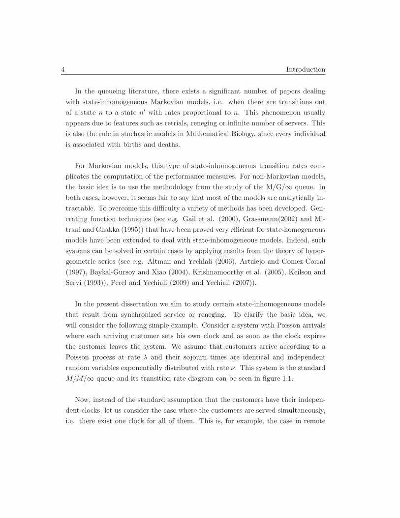
In the present dissertation we aim to study certain state-inhomogeneous models
that result from synchronized service or reneging. To clarify the basic idea, we
will consider the following simple example. Consider a system with Poisson arrivals
where each arriving customer sets his own clock and as soon as the clock expires
the customer leaves the system. We assume that customers arrive according to a
Poisson process at rate " and their sojourn times are identical and independent
random variables exponentially distributed with rate #. This system is the standard
M/M/# queue and its transition rate diagram can be seen in figure 1.1.
Now, instead of the standard assumption that the customers have their indepen-
dent clocks, let us consider the case where the customers are served simultaneously,
i.e. there exist one clock for all of them. This is, for example, the case in remote
1.1 Background and motivation 5
0"
## 1
!
$$
"## 2
2!
$$
"## 3
3!
$$
"## · · ·
4!
%%
Fig. 1.1: Transition rate diagram for the M/M/# queue
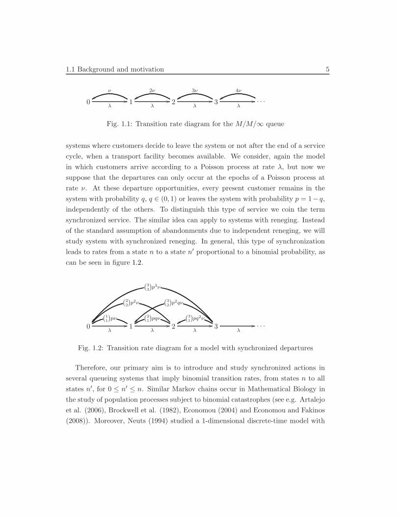
systems where customers decide to leave the system or not after the end of a service
cycle, when a transport facility becomes available. We consider, again the model
in which customers arrive according to a Poisson process at rate ", but now we
suppose that the departures can only occur at the epochs of a Poisson process at
rate #. At these departure opportunities, every present customer remains in the
system with probability q, q % (0, 1) or leaves the system with probability p = 1! q,
independently of the others. To distinguish this type of service we coin the term
synchronized service. The similar idea can apply to systems with reneging. Instead
of the standard assumption of abandonments due to independent reneging, we will
study system with synchronized reneging. In general, this type of synchronization
leads to rates from a state n to a state n" proportional to a binomial probability, as
can be seen in figure 1.2.
0"
## 1(11)p!$$
"## 2
(21)pq!
$$
(22)p
2!
&&
"## 3
(31)pq2!
$$
(32)p
2q!
&&
(33)p
3!
''
"## · · ·
Fig. 1.2: Transition rate diagram for a model with synchronized departures
Therefore, our primary aim is to introduce and study synchronized actions in
several queueing systems that imply binomial transition rates, from states n to all
states n", for 0 & n" & n. Similar Markov chains occur in Mathematical Biology in
the study of population processes subject to binomial catastrophes (see e.g. Artalejo
et al. (2006), Brockwell et al. (1982), Economou (2004) and Economou and Fakinos
(2008)). Moreover, Neuts (1994) studied a 1-dimensional discrete-time model with
6 Introduction
similar dynamics.
We will concentrate on 2-dimensional queueing systems with synchronized ser-
vices and synchronized abandonments. We first study systems with synchronized
services as a variation/extension of the model with infinite servers. However, the
synchronization increases the complexity for obtaining the stationary distribution
of the system as well as the other performance measures, such as the distribution of
the sojourn time and the busy period analysis.
We then proceed to the modeling and analysis of queueing systems with syn-
chronized reneging. The idea of customers independent reneging goes back to the
pioneering work of Palm (1953, 1957) who was the first to study the M/M/c queue
with exponential patience times. Another important researcher was Daley (1965),
who did some important work on the GI/G/1 queue with independent reneging.
Takacs (1974) considered the M/G/1 queue with a threshold waiting time, where
the customers leave the system as soon as this threshold is exceeded. Later on,
Boxma and de Waal (1994) studied the M/M/c queue with generally distributed
patience times.
Recently, several authors studied the case of queueing systems where customers
reneging is associated with the temporal absence of the server. We refer to mod-
els in which the server becomes temporarily unavailable as server vacation models.
Typically a vacation of the server starts as soon as the system remains empty after
the end of a busy period. We refer to the time interval during which the server
is unavailable as a vacation period. A vacation period is usually terminated by a
condition that depends on the arrival process during that vacation period. For ex-
ample, in some situations it is reasonable to assume that the server takes multiple
vacations as long as the system remain empty, while in other situations it seems
better to assume that the server takes only a single vacation and then stays in the
system ready to serve, even when there are no waiting customers. In other sys-
tems, the vacations happen because of random failures of the server (servers with
on-o" periods, unreliable servers, servers with failures and repairs). Models based
1.1 Background and motivation 7
on the M/G/1 queue with vacations were studied by Altiok (1987), Cooper (1970),
Fuhrmann (1984), Harris and Marshal (1988), Levy and Yechiali (1975), Shaked
and Shanthikumar (1986), Yadin and Naor (1963), and many others. If we add
the feature of independent reneging to a vacation model, we have a model that is
referred to as a server vacation model with independent reneging. These models
reflect human behavior in certain real life situations and were initially introduced
by Altman and Yechiali (2006). In this thesis, we aim to extend their framework by
introducing and analyzing server vacation models with synchronized abandonments.
Another source for customer impatience is the possible failures of the system.
Cases in which the service of the customers is interrupted by some random mech-
anism were initially studied for single server systems, (see e.g. Gaver (1962) and
Keilson (1962)) and then extended to the multiple servers case (see e.g. Mitrany
and Avi-Itzhab (1968)).
Introducing the e"ect of synchronization and using generating function tech-
niques to obtain the probability generating function of the number of customers in
the system usually leads to systems that can be solved by applying the theory of
q–hypergeometric series, known also as basic hypergeometric series (see Gasper and
Rahman (2004)). However, in the queueing theory literature, there exists only few
papers where this theory has been applied (see e.g. Ismail (1985), Kemp (1990,
1992, 1998, 2005)).
We will show that models with synchronized actions represent more realistically
some service systems and that the framework of q–hypergeometric series enables us
to express in closed form the main performance measures of such a system. In gen-
eral, the theory of q–hypergeometric series can facilitate the computations regarding
systems with this kind of binomial transitions arising from synchronization.
There exists a rich theory for the class of q–hypergeometric series and their q–
calculus which enables fast calculations and simplifications. For this reason and
for the sake of self-completeness we will briefly summarize the basic definitions and
8 Introduction
results of this theory in the next section. The interested reader can find more details
on the definitions and the results below (with proofs and extensions) in Gasper and
Rahman (2004), Chapters 1-3 and Appendices I-III.
1.2 Basic Hypergeometric series
Basic hypergeometric series are series of the form!#
n=0 un where u0 = 1 and un+1
un
a rational function of qn for a deformation parameter q, which is usually taken to
satisfy |q| < 1. They were initially introduced by Heine who developed their basic
theory, following Gauss’ fundamental paper on hypergeometric series.
Observing that the ratio un+1/un, being rational in qn, can be written in the form
un+1
un=
(1 ! a1qn)(1 ! a2qn) · · · (1 ! arqn)
(1 ! qn+1)(1 ! b1qn) · · · (1 ! bsqn)(!qn)1+s$rz, (1.1)
we have that every such series assumes the form
r!s
"
a1, a2, . . . , ar
b1, . . . , bs; q, z
#
' r!s(a1, a2, . . . , ar; b1, b2, . . . , bs; q; z)
=#$
n=0
(a1; q)n(a2; q)n · · · (ar; q)n(q; q)n(b1; q)n · · · (bs; q)n
%
(!1)nq(n2)&1+s$r
zn ,
(1.2)
where (a; q)n is referred as the q–shifted factorial and is given as
(a; q)n =
'
(
)
1, n = 0
(1 ! a)(1 ! aq)(1 ! aq2) · · · (1 ! aqn$1), n = 1, 2, . . . .
It is assumed in the definition of the r!s series, equation (1.2), that bi (= q$m for
m = 0, 1, . . . and for every i = 1, 2, . . . , s. Using the ratio test, for 0 < |q| < 1,
we can easily see that the r!s series converges for all z if r & s and for |z| < 1 if
r = s + 1. In what follows it is assumed that 0 < q < 1.
We also define
(a; q)# =#*
i=0
(1 ! aqi).
1.2 Basic Hypergeometric series 9
The following easily derived identities will be frequently used in this manuscript:
(a; q)n =(a; q)#
(aqn; q)#(1.3)
(a$1q1$n; q)n = (a; q)n(!a$1)nq$(n2). (1.4)
Since products of q–shifted factorials occur so often, to simplify them we shall fre-
quently use the more compact notations
(a1, a2, . . . , am; q)n = (a1; q)n(a2; q)n · · · (am; q)n
(a1, a2, . . . , am; q)# = (a1; q)#(a2; q)# · · · (am; q)#.
1.2.1 The q–binomial theorem
A q–calculus has been developed that parallels the theory of hypergeometric func-
tions. The most important summation formula for the q–hypergeometric series is
given by the q–binomial theorem
1!0(a;!; q; z) =#$
n=0
(a; q)n(q; q)n
zn =(az; q)#(z; q)#
, |z| < 1. (1.5)
Of particular importance are the two q–analogues of the exponential function ez .
They are the functions eq(z) = 1(z;q)"
and Eq(z) = (!z; q)#. The q–binomial
theorem enables to express the q–exponential functions in the form of q–series. If
we set a = 0 in (1.5) we get
eq(z) = 1!0(0;!; q; z) =#$
n=0
zn
(q; q)n=
1
(z; q)#, |z| < 1. (1.6)
If we replace z by ! za in (1.5) and then let a " # to get
Eq(z) = 0!0(!;!; q; z) =#$
n=0
q(n2)
(q; q)nzn = (!z; q)#. (1.7)
10 Introduction
We observe that, as q " 1$ the q–analogues reduce to their standard counterparts.
In particular we have the relationships
limq%1!
eq(z(1 ! q)) = ez (1.8)
limq%1!
Eq(z(1 ! q)) = ez (1.9)
limq%1!
(qaz; q)#(z; q)#
= (1 ! z)$a. (1.10)
1.2.2 Transformation formulas for 2!1 series
Heine (1847,1878) showed that
2!1(a, b; c; q, z) =(b, az; q)#(c, z; q)#
2!1(c/b, z; az; q, b) (1.11)
=(c/b, bz; q)#
(c, z; q)#2!1(abz/c, b; bz; q, c/b) (1.12)
=(abz/c; q)#
(z; q)#2!1(c/a, c/b; c; q, abz/c). (1.13)
Jackson (1910) proved that
2!1(a, b; c; q, z) =(az; q)#(z; q)#
2!2(a, c/b; c, az; q, bz). (1.14)
1.2.3 The q–integral
Finally Thomae (1869,1870) and Jackson (1910,1951) introduced the q–integral
+ 1
0f(t)dqt = (1 ! q)
#$
n=0
f(qn)qn (1.15)
and Jackson gave the most general definition+ b
af(t)dqt =
+ b
of(t)dqt !
+ a
0f(t)dqt, (1.16)
where+ a
0f(t)dqt = a(1 ! q)
#$
n=0
f(aqn)qn. (1.17)
1.3 Overview of the thesis 11
If f is continuous on [0, a], then it is easily seen that
limq%1!
+ a
0f(t)dqt =
+ a
0f(t)dt. (1.18)
We will use the q–integral convergence to the ordinary integral to prove limiting
results in the case when q " 1$, since a r+1!r series can be expressed as a q–
integral through the relation
r+1!r
"
a1, . . . , ar+1
b1, . . . , br; q, qz
#
=(a1, . . . , ar+1; q)#
(1 ! q)(q, b1, . . . , br; q)#
)+ 1
0tz$1 (qt, b1t, . . . , brt; q)#
(a1t, . . . , ar+1t; q)#dqt, (1.19)
when Rez > 0, and the series on the left side does not terminate.
1.2.4 Limiting regimes as q " 0+
As q " 0+ we can easily see that
limq%0+
eq(z) =1
1 ! z(1.20)
limq%0+
Eq(z) = 1 + z. (1.21)
We can also prove the limiting relation
limq%0+
r+1!r
"
a1, · · · , ar+1
b1, · · · , br; q, q
#
= 1. (1.22)
1.3 Overview of the thesis
This thesis is organized according to the specific models that we study. More con-
cretely, in every chapter we first motivate the model under consideration and then
describe the previous contributions reported in the literature. Subsequently, we
provide a mathematical description of the model and begin to study several perfor-
mance measures such as the stationary distribution of the system state, the sojourn
time and the busy period distributions. Several mean performance measures are
12 Introduction
also considered and studied. We also report results concerning the behavior of the
model under several limiting regimes.
In chapter 2, we consider a single server Markovian queue with synchronized
services and setup times. Customers arrive according to a Poisson process and are
served simultaneously. At a service completion epoch, every customer remains sat-
isfied with probability p (independently of the others) and departs from the system;
otherwise he stays for a new service. Moreover, the server takes multiple vacations
whenever the system is empty. To study the model we introduce a 2-dimensional
Markov chain and observe that the transition rates of the underlying Markov chain
are state-inhomogeneous, because the number of customers n is reduced according
to a binomial (n, p) distribution at each service completion epoch. We show that
the model can be e!ciently studied using the framework of q-hypergeometric series
and we carry out an extensive analysis including the stationary, the busy period and
the sojourn time distributions. Exact formulas and numerical results show the e"ect
of the level of synchronization to the performance of the system. More concretely,
chapter 2 is organized as follows: In section 2.2 we describe the model and introduce
the appropriate notation. In section 2.3 we carry out the equilibrium analysis of the
system state with the use of partial probability generating functions and we derive
several exact formulas and iterative algorithmic schemes. Some limiting regimes are
discussed in more detail. The busy period and sojourn time distributions are studied
in section 2.4. Finally, in section 2.5, we provide several numerical studies and we
discuss the e"ect of the level of synchronization on the system performance.
In chapter 3 we consider a single server unreliable queue represented by a 2-
dimensional continuous time Markov chain. Customers arrive according to a Poisson
process and find the server in one of two modes: on or o". The server is subject
to failures that remove all present customers from the system. Moreover, as long
as the server is down, we assume that the arrivals continue to come, but the cus-
tomers become impatient and perform synchronized abandonments. This model was
motivated by remote systems where customers have to wait for a certain transport
facility to abandon the system. Then, whenever the facility visits the system, the
1.3 Overview of the thesis 13
present customers can decide whether to leave the system or not. More specifically,
we assume that the abandonment opportunities occur according to a Poisson pro-
cess, whenever the server is down (so we can think that the transportation facility’s
arrivals occur according to this process). Then, at an abandonment opportunity
epoch, every customer decides to abandon the system with probability p or remains
in the system waiting for service with probability q = 1 ! p, independently of the
others. In section 3.2 we describe the model and introduce the appropriate notation.
In section 3.3 we carry out the equilibrium analysis of the system state and derive
several exact formulas and iterative algorithmic schemes. Some limiting regimes
with a particular interest are discussed in more detail. In section 3.4 we study the
conditional mean sojourn times of a customer, while in section 3.5 we treat the sys-
tem busy period distribution of the model.
In chapters 4 and 5 we present a detailed analysis of two fundamental queueing
models with vacations and impatient customers, where the source of the impatience
is the absence of the server. Instead of the standard assumption that customers
perform independent abandonments, we consider situations where customers aban-
don the system simultaneously. In chapter 4 we study the Markovian case, while in
chapter 5 we study the non-Markovian counterparts. In both chapters we study two
models. The first model is the single-server queue with multiple vacations, where
customers decide whether to abandon the system or not when the vacation periods
finish. In the second model, we suppose that the abandonments opportunities oc-
cur according to a Poisson process during vacation periods. At the abandonment
opportunities, every present customer remains in the system with probability q or
abandons the system with probability p = 1! q, independently of the others. Chap-
ter 4 is organized as follows: In section 4.2, we describe the dynamics of the models.
In section 4.3 we carry out a mean value analysis of the two Markovian models. In
section 4.4 we present, separately, the stationary analysis of the two models. We
also obtain more explicit results under various limiting regimes concerning the pa-
rameters of the models. Along the same lines, chapter 5 is organized as follows: In
section 5.2, we describe the dynamics of the models. In section 5.3 we carry out a
mean value analysis of the two models, while in section 5.4 we study their station-
14 Introduction
ary distributions by using a generating function approach. In section 5.5 we present
several numerical results that illustrate the e"ect of the various parameters on the
performance measures of the model.
Chapter 2
Synchronized services in a
single server vacation queue
We consider a single server Markovian queue with synchronized services and setup
times. Customers arrive according to a Poisson process and are served simultane-
ously. At a service completion epoch, every customer remains satisfied with prob-
ability p (independently of the others) and departs from the system; otherwise he
stays for a new service. Moreover, the server takes multiple vacations whenever the
system is empty.
The transition rates of the underlying 2-dimensional Markov chain are state - in-
homogeneous, because the number of customers n is reduced according to a binomial
(n, p) distribution at each service completion epoch. We show that the model can
be e!ciently studied using the framework of q-hypergeometric series and we carry
out an extensive analysis including the stationary, the busy period and the sojourn
time distributions. Exact formulas and numerical results show the e"ect of the level
of synchronization to the performance of such systems.
16 Synchronized services in a single server vacation queue
2.1 Introduction
In the queueing literature, there exists a significant number of papers dealing with
2-dimensional Markovian models. In this kind of queueing models, the state of the
system is represented by a vector (n, i), where n records the number of customers,
while i gives information about some special feature of the system (e.g. state of the
server(s), number of priority customers, phase of the arrival or the service process
etc.). These models have received considerable attention, because on the one hand
they can easily represent various queueing characteristics and on the other hand
many of them are analytically tractable, thus providing e"ective computations of
performance measures.
However, most of the analytically tractable models have two limitations: First,
only one of the two variables is unlimited (usually the number of customers), while
the other is assumed to take only a finite number of values. Second, the underlying
Markov chain exhibits -at least to a certain degree- spatial homogeneity. A variety
of methods has been developed for such models. Matrix analytic methods (see e.g.
Bini et al. (2005), Latouche and Ramaswami (1999) and Neuts (1981, 1989)) and
generating function techniques (see e.g. Gail et al. (2000), Grassmann(2002) and
Mitrani and Chakka (1995)) have been proved very e!cient.
In systems that do not satisfy the above constraints the analysis is much more
complicate. When only the first constraint is violated, that is both variables are
unlimited but the Markov chain is space-homogeneous, the matrix analytic methods
still apply, although there exist serious di!culties (see e.g. Kroese et al. (2004)).
An alternative is to use analytic tools. One widely used approach is the reduction
to a Riemann-Hilbert boundary value problem (see e.g. Cohen and Boxma (1983)).
The compensation method (Adan(1991)) has also been used for the e!cient solution
of a number of models.
The second constraint, that is the spatial homogeneity, is usually violated due
to features such as retrials, reneging or infinite number of servers. Indeed, in these
2.1 Introduction 17
situations, there are transitions out of a state (n, i) to a state (n ! 1, i") with rates
proportional to n. This is also the rule in stochastic models in Mathematical Bi-
ology, since every individual is associated with births and deaths. There are only
few works trying to extend matrix analytic methods within this framework. In most
cases the authors use truncation or generalized truncation ideas to study the sys-
tems (see e.g. Artalejo and Pozo (2002) and the references therein) or they apply
generating function methods. However, we have to note that in this case the partial
generating functions of the number of individuals in system satisfy a system of linear
di"erential equations in contrast with the state homogeneous case where they satisfy
linear algebraic equations. Such systems are usually intractable or can be solved in
terms of hypergeometric series (see e.g. Altman and Yechiali (2006), Artalejo and
Gomez-Corral (1997), Baykal-Gursoy and Xiao (2004), Keilson and Servi (1993) and
Krishnamoorthy et al. (2005) ).
The primary aim of this chapter is the study of a synchronization characteristic
that also leads to spatially inhomogeneous Markov chains. Indeed, suppose that
all the n present customers of a given system are served concurrently, according to
an exponential distribution with parameter µ. If at the service completion epoch
every customer is satisfied and departs with probability p or repeats his service with
probability q, independently of the others, then there are binomial transition rates
of the form µ,nn#
-
pn$n#qn#
, from a state (n, i) to states (n", i), for 0 & n" & n. Similar
Markov chains occur in Mathematical Biology in the study of population processes
subject to binomial catastrophes (see e.g. Artalejo et al. (2006), Brockwell et al.
(1982), Economou (2004) and Economou and Fakinos (2009) ). Moreover, Neuts
(1994) studied a 1-dimensional discrete-time model with similar dynamics.
The model of this chapter is a queueing system with synchronized services and
setup times (also known as multiple server’s vacations). The literature on queueing
systems with vacations is vast (see e.g. Takagi (1991), Tian and Zhang (2006) and
the references therein). However, to the best of our knowledge, there are no papers
dealing with vacation queueing systems with some kind of synchronization. A po-
tential application of this type of models is the representation of distance-learning
18 Synchronized services in a single server vacation queue
service systems (e.g. webseminars), where all customers are served concurrently and
then decide independently whether to repeat their service or not.
The chapter is organized as follows. In section 2.2 we describe the model and
introduce the appropriate notation. In section 2.3 we carry out the equilibrium
analysis of the system state and we derive several exact formulas and iterative al-
gorithmic schemes. Some limiting regimes are discussed in more detail. The busy
period and sojourn time distributions are studied in section 2.4. Finally, in section
2.5, we provide several numerical studies and we discuss the e"ect of the level of
synchronization to the system performance.
2.2 Model description and notation
We consider a queueing system in which customers arrive according to a Poisson
process at rate ". The service is provided by a single server, who serves simultane-
ously all present customers. The successive service times of the server are assumed
to be exponential random variables with rate µ. At a service completion epoch,
each customer is satisfied and departs with probability p or repeats his service with
probability q = 1 ! p, independently of the others. Whenever the system becomes
empty, the server is deactivated immediately. As soon as an arrival enters to an
empty system, the server begins a setup time to reactivate. The setup times are
exponentially distributed at rate $. An alternative interpretation is that the server
takes exponentially distributed multiple vacations with parameter $ as long as the
system remains empty.
The system is represented by a continuous-time Markov chain {(N(t), I(t)) : t $0}, where N(t) is the number of customers in the system at time t and I(t) denotes
the state of the server at time t (0=o" and 1=on), t $ 0. The corresponding
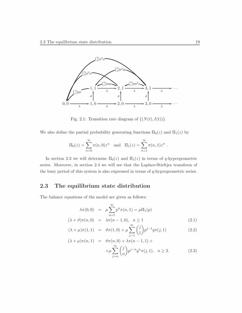
transition diagram is given in Figure 2.1.
Let (%(n, i) : i = 0, 1 and n $ i) denote the stationary distribution of {(N(t), I(t))}.
2.3 The equilibrium state distribution 19
1, 1(11)pµ
((
"## 2, 1
(21)pqµ))
(22)p2µ
**
"## 3, 1
(31)pq2µ))
(32)p
2qµ
++
(33)p3µ
,,
"## · · ·
0, 0"
## 1, 0
#
--
"## 2, 0
#
--
"## 3, 0
#
--
"## · · ·
Fig. 2.1: Transition rate diagram of {(N(t), I(t))}.
We also define the partial probability generating functions #0(z) and #1(z) by
#0(z) =#$
n=0
%(n, 0)zn and #1(z) =#$
n=1
%(n, 1)zn .
In section 2.3 we will determine #0(z) and #1(z) in terms of q-hypergeometric
series. Moreover, in section 2.4 we will see that the Laplace-Stieltjes transform of
the busy period of this system is also expressed in terms of q-hypergeometric series.
2.3 The equilibrium state distribution
The balance equations of the model are given as follows:
"%(0, 0) = µ#$
n=1
pn%(n, 1) = µ#1(p)
(" + $)%(n, 0) = "%(n ! 1, 0), n $ 1 (2.1)
(" + µ)%(1, 1) = $%(1, 0) + µ#$
j=1
.
j
1
/
pj$1q%(j, 1) (2.2)
(" + µ)%(n, 1) = $%(n, 0) + "%(n ! 1, 1) +
+µ#$
j=n
.
j
n
/
pj$nqn%(j, 1), n $ 2. (2.3)
20 Synchronized services in a single server vacation queue
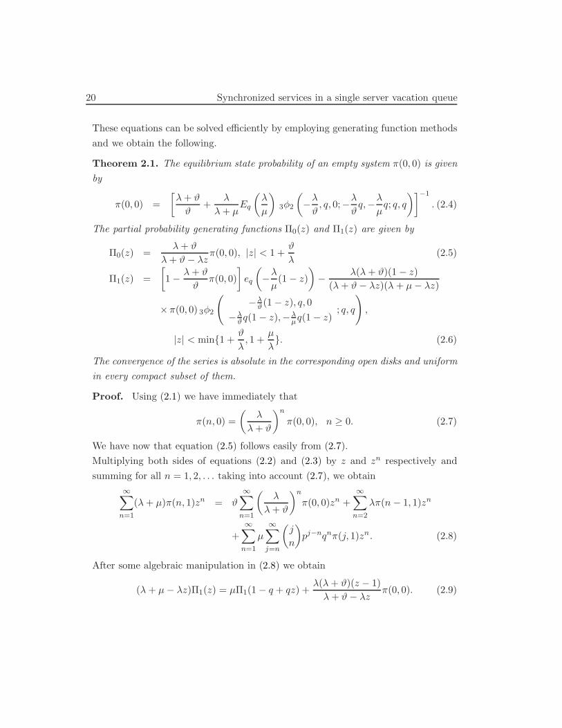
These equations can be solved e!ciently by employing generating function methods
and we obtain the following.
Theorem 2.1. The equilibrium state probability of an empty system %(0, 0) is given
by
%(0, 0) =
0
" + $
$+
"
" + µEq
.
"
µ
/
3!2
.
!"
$, q, 0;!
"
$q,!
"
µq; q, q
/1$1
. (2.4)
The partial probability generating functions #0(z) and #1(z) are given by
#0(z) =" + $
" + $! "z%(0, 0), |z| < 1 +
$
"(2.5)
#1(z) =
0
1 !" + $
$%(0, 0)
1
eq
.
!"
µ(1 ! z)
/
!"(" + $)(1 ! z)
(" + $! "z)(" + µ ! "z)
)%(0, 0) 3!2
"
!"#(1 ! z), q, 0
!"#q(1 ! z),!"µq(1 ! z); q, q
#
,
|z| < min{1 +$
", 1 +
µ
"}. (2.6)
The convergence of the series is absolute in the corresponding open disks and uniform
in every compact subset of them.
Proof. Using (2.1) we have immediately that
%(n, 0) =
.
"
" + $
/n
%(0, 0), n $ 0. (2.7)
We have now that equation (2.5) follows easily from (2.7).
Multiplying both sides of equations (2.2) and (2.3) by z and zn respectively and
summing for all n = 1, 2, . . . taking into account (2.7), we obtain
#$
n=1
(" + µ)%(n, 1)zn = $#$
n=1
.
"
" + $
/n
%(0, 0)zn +#$
n=2
"%(n ! 1, 1)zn
+#$
n=1
µ#$
j=n
.
j
n
/
pj$nqn%(j, 1)zn. (2.8)
After some algebraic manipulation in (2.8) we obtain
(" + µ ! "z)#1(z) = µ#1(1 ! q + qz) +"(" + $)(z ! 1)
" + $! "z%(0, 0). (2.9)
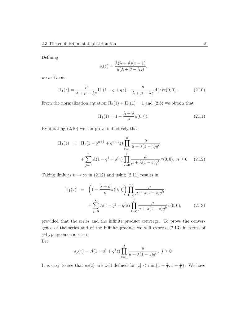
2.3 The equilibrium state distribution 21
Defining
A(z) ="(" + $)(z ! 1)
µ(" + $! "z),
we arrive at
#1(z) =µ
" + µ ! "z#1(1 ! q + qz) +
µ
" + µ ! "zA(z)%(0, 0). (2.10)
From the normalization equation #0(1) + #1(1) = 1 and (2.5) we obtain that
#1(1) = 1 !" + $
$%(0, 0). (2.11)
By iterating (2.10) we can prove inductively that
#1(z) = #1(1 ! qn+1 + qn+1z)n*
k=0
µ
µ + "(1 ! z)qk
+n$
j=0
A(1 ! qj + qjz)j*
k=0
µ
µ + "(1 ! z)qk%(0, 0), n $ 0. (2.12)
Taking limit as n " # in (2.12) and using (2.11) results in
#1(z) =
.
1 !" + $
$%(0, 0)
/ #*
k=0
µ
µ + "(1 ! z)qk
+#$
j=0
A(1 ! qj + qjz)j*
k=0
µ
µ + "(1 ! z)qk%(0, 0), (2.13)
provided that the series and the infinite product converge. To prove the conver-
gence of the series and of the infinite product we will express (2.13) in terms of
q–hypergeometric series.
Let
aj(z) = A(1 ! qj + qjz)j*
k=0
µ
µ + "(1 ! z)qk, j $ 0.
It is easy to see that aj(z) are well defined for |z| < min{1 + #" , 1 + µ
"}. We have
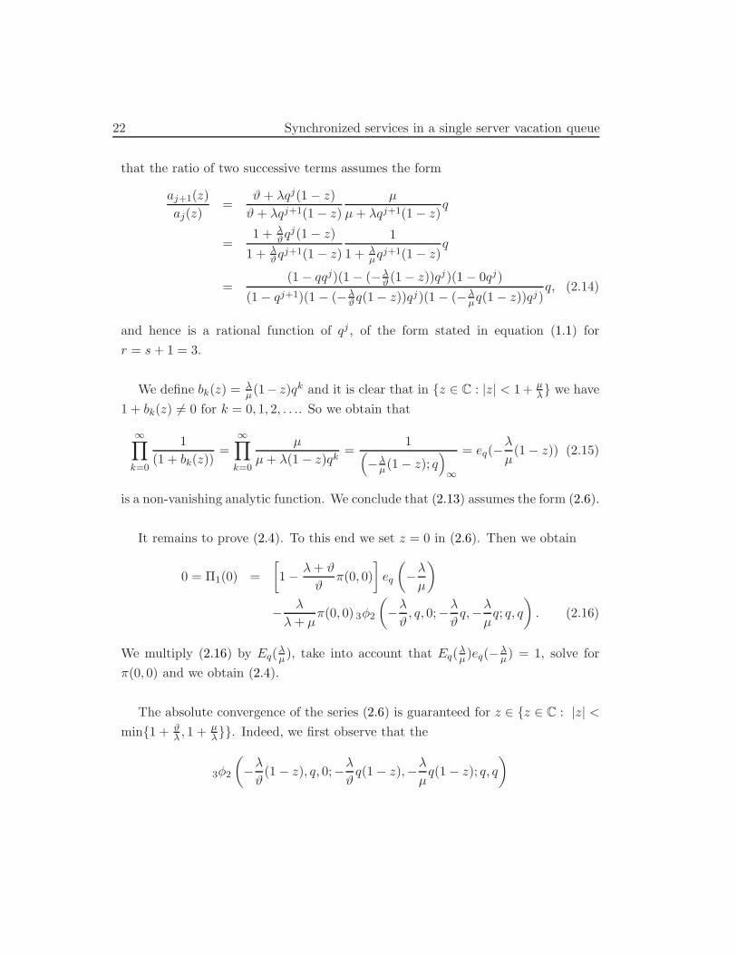
22 Synchronized services in a single server vacation queue
that the ratio of two successive terms assumes the form
aj+1(z)
aj(z)=
$ + "qj(1 ! z)
$ + "qj+1(1 ! z)
µ
µ + "qj+1(1 ! z)q
=1 + "
#qj(1 ! z)
1 + "#q
j+1(1 ! z)
1
1 + "µqj+1(1 ! z)
q
=(1 ! qqj)(1 ! (!"#(1 ! z))qj)(1 ! 0qj)
(1 ! qj+1)(1 ! (!"#q(1 ! z))qj)(1 ! (!"µq(1 ! z))qj)q, (2.14)
and hence is a rational function of qj , of the form stated in equation (1.1) for
r = s + 1 = 3.
We define bk(z) = "µ(1! z)qk and it is clear that in {z % C : |z| < 1+ µ
"} we have
1 + bk(z) (= 0 for k = 0, 1, 2, . . .. So we obtain that
#*
k=0
1
(1 + bk(z))=
#*
k=0
µ
µ + "(1 ! z)qk=
12
!"µ(1 ! z); q3
#
= eq(!"
µ(1 ! z)) (2.15)
is a non-vanishing analytic function. We conclude that (2.13) assumes the form (2.6).
It remains to prove (2.4). To this end we set z = 0 in (2.6). Then we obtain
0 = #1(0) =
0
1 !" + $
$%(0, 0)
1
eq
.
!"
µ
/
!"
" + µ%(0, 0) 3!2
.
!"
$, q, 0;!
"
$q,!
"
µq; q, q
/
. (2.16)
We multiply (2.16) by Eq("µ), take into account that Eq(
"µ)eq(!"µ) = 1, solve for
%(0, 0) and we obtain (2.4).
The absolute convergence of the series (2.6) is guaranteed for z % {z % C : |z| <
min{1 + #" , 1 + µ
"}}. Indeed, we first observe that the
3!2
.
!"
$(1 ! z), q, 0;!
"
$q(1 ! z),!
"
µq(1 ! z); q, q
/
2.3 The equilibrium state distribution 23
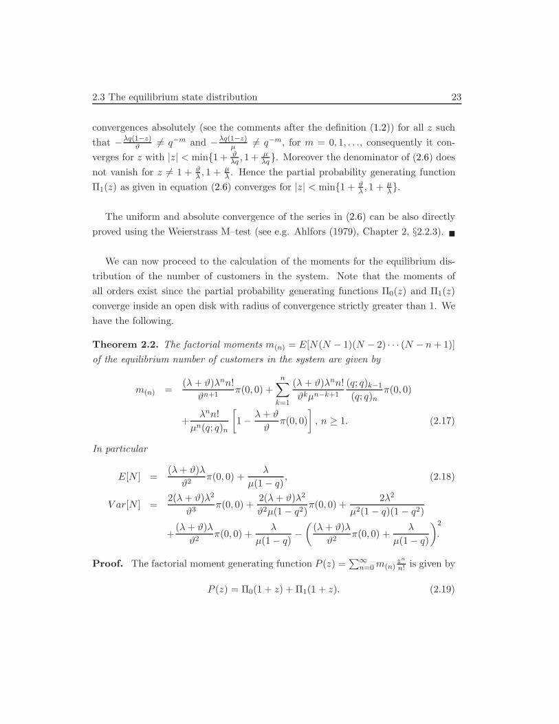
convergences absolutely (see the comments after the definition (1.2)) for all z such
that !"q(1$z)# (= q$m and !"q(1$z)
µ (= q$m, for m = 0, 1, . . ., consequently it con-
verges for z with |z| < min{1 + #"q , 1 + µ
"q}. Moreover the denominator of (2.6) does
not vanish for z (= 1 + #" , 1 + µ
" . Hence the partial probability generating function
#1(z) as given in equation (2.6) converges for |z| < min{1 + #" , 1 + µ
"}.
The uniform and absolute convergence of the series in (2.6) can be also directly
proved using the Weierstrass M–test (see e.g. Ahlfors (1979), Chapter 2, §2.2.3). !
We can now proceed to the calculation of the moments for the equilibrium dis-
tribution of the number of customers in the system. Note that the moments of
all orders exist since the partial probability generating functions #0(z) and #1(z)
converge inside an open disk with radius of convergence strictly greater than 1. We
have the following.
Theorem 2.2. The factorial moments m(n) = E[N(N ! 1)(N ! 2) · · · (N ! n + 1)]
of the equilibrium number of customers in the system are given by
m(n) =(" + $)"nn!
$n+1%(0, 0) +
n$
k=1
(" + $)"nn!
$kµn$k+1
(q; q)k$1
(q; q)n%(0, 0)
+"nn!
µn(q; q)n
0
1 !" + $
$%(0, 0)
1
, n $ 1. (2.17)
In particular
E[N ] =(" + $)"
$2%(0, 0) +
"
µ(1 ! q), (2.18)
V ar[N ] =2(" + $)"2
$3%(0, 0) +
2(" + $)"2
$2µ(1 ! q2)%(0, 0) +
2"2
µ2(1 ! q)(1 ! q2)
+(" + $)"
$2%(0, 0) +
"
µ(1 ! q)!.
(" + $)"
$2%(0, 0) +
"
µ(1 ! q)
/2
.
Proof. The factorial moment generating function P (z) =!#
n=0 m(n)zn
n! is given by
P (z) = #0(1 + z) + #1(1 + z). (2.19)
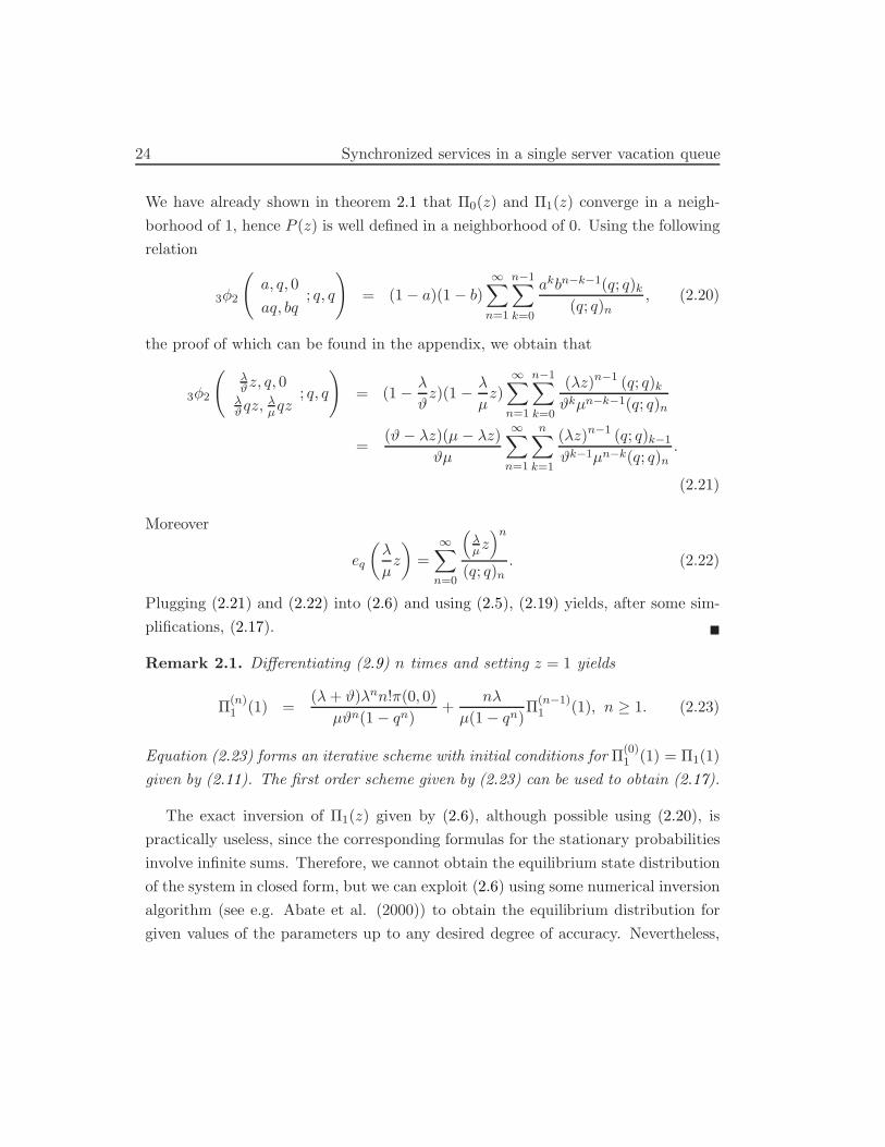
24 Synchronized services in a single server vacation queue
We have already shown in theorem 2.1 that #0(z) and #1(z) converge in a neigh-
borhood of 1, hence P (z) is well defined in a neighborhood of 0. Using the following
relation
3!2
"
a, q, 0
aq, bq; q, q
#
= (1 ! a)(1 ! b)#$
n=1
n$1$
k=0
akbn$k$1(q; q)k(q; q)n
, (2.20)
the proof of which can be found in the appendix, we obtain that
3!2
"
"#z, q, 0"#qz, "µqz
; q, q
#
= (1 !"
$z)(1 !
"
µz)
#$
n=1
n$1$
k=0
("z)n$1 (q; q)k$kµn$k$1(q; q)n
=($! "z)(µ ! "z)
$µ
#$
n=1
n$
k=1
("z)n$1 (q; q)k$1
$k$1µn$k(q; q)n.
(2.21)
Moreover
eq
.
"
µz
/
=#$
n=0
2
"µz3n
(q; q)n. (2.22)
Plugging (2.21) and (2.22) into (2.6) and using (2.5), (2.19) yields, after some sim-
plifications, (2.17). !
Remark 2.1. Di!erentiating (2.9) n times and setting z = 1 yields
#(n)1 (1) =
(" + $)"nn!%(0, 0)
µ$n(1 ! qn)+
n"
µ(1 ! qn)#(n$1)
1 (1), n $ 1. (2.23)
Equation (2.23) forms an iterative scheme with initial conditions for #(0)1 (1) = #1(1)
given by (2.11). The first order scheme given by (2.23) can be used to obtain (2.17).
The exact inversion of #1(z) given by (2.6), although possible using (2.20), is
practically useless, since the corresponding formulas for the stationary probabilities
involve infinite sums. Therefore, we cannot obtain the equilibrium state distribution
of the system in closed form, but we can exploit (2.6) using some numerical inversion
algorithm (see e.g. Abate et al. (2000)) to obtain the equilibrium distribution for
given values of the parameters up to any desired degree of accuracy. Nevertheless,
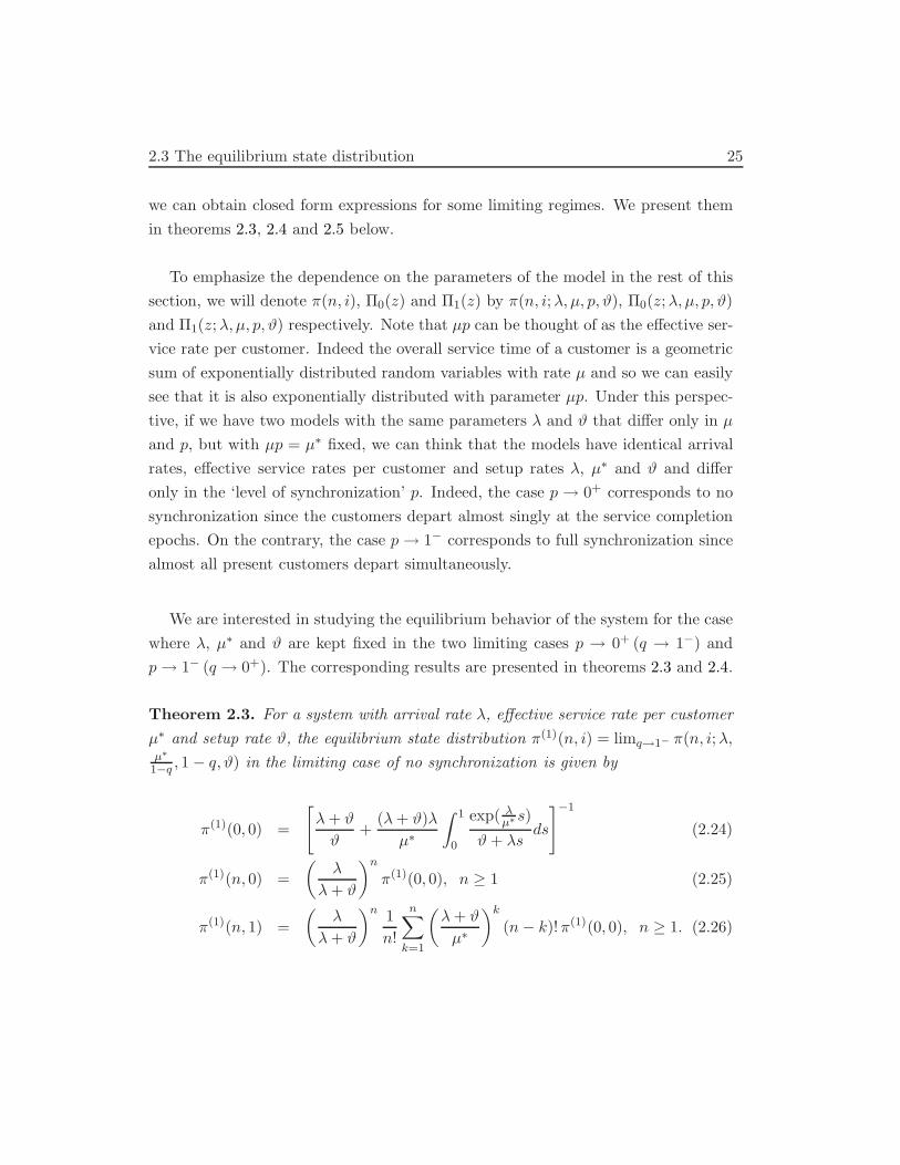
2.3 The equilibrium state distribution 25
we can obtain closed form expressions for some limiting regimes. We present them
in theorems 2.3, 2.4 and 2.5 below.
To emphasize the dependence on the parameters of the model in the rest of this
section, we will denote %(n, i), #0(z) and #1(z) by %(n, i;", µ, p,$), #0(z;", µ, p,$)
and #1(z;", µ, p,$) respectively. Note that µp can be thought of as the e"ective ser-
vice rate per customer. Indeed the overall service time of a customer is a geometric
sum of exponentially distributed random variables with rate µ and so we can easily
see that it is also exponentially distributed with parameter µp. Under this perspec-
tive, if we have two models with the same parameters " and $ that di"er only in µ
and p, but with µp = µ& fixed, we can think that the models have identical arrival
rates, e"ective service rates per customer and setup rates ", µ& and $ and di"er
only in the ‘level of synchronization’ p. Indeed, the case p " 0+ corresponds to no
synchronization since the customers depart almost singly at the service completion
epochs. On the contrary, the case p " 1$ corresponds to full synchronization since
almost all present customers depart simultaneously.
We are interested in studying the equilibrium behavior of the system for the case
where ", µ& and $ are kept fixed in the two limiting cases p " 0+ (q " 1$) and
p " 1$ (q " 0+). The corresponding results are presented in theorems 2.3 and 2.4.
Theorem 2.3. For a system with arrival rate ", e!ective service rate per customer
µ& and setup rate $, the equilibrium state distribution %(1)(n, i) = limq%1! %(n, i;",µ$
1$q , 1 ! q,$) in the limiting case of no synchronization is given by
%(1)(0, 0) =
4
" + $
$+
(" + $)"
µ&
+ 1
0
exp( "µ$ s)
$ + "sds
5$1
(2.24)
%(1)(n, 0) =
.
"
" + $
/n
%(1)(0, 0), n $ 1 (2.25)
%(1)(n, 1) =
.
"
" + $
/n 1
n!
n$
k=1
.
" + $
µ&
/k
(n ! k)!%(1)(0, 0), n $ 1. (2.26)
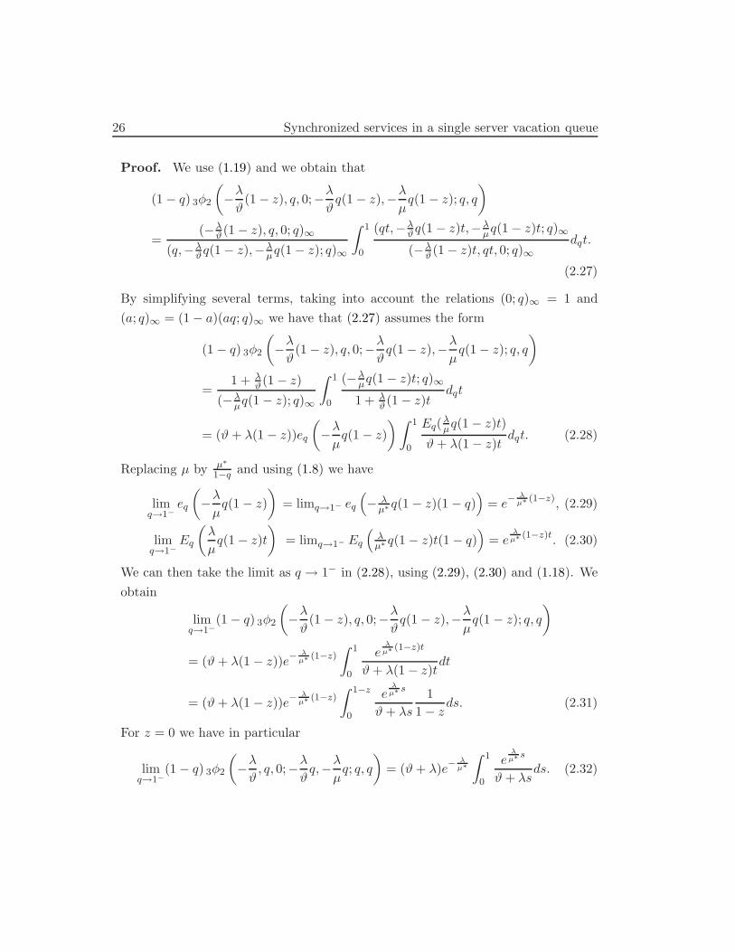
26 Synchronized services in a single server vacation queue
Proof. We use (1.19) and we obtain that
(1 ! q) 3!2
.
!"
$(1 ! z), q, 0;!
"
$q(1 ! z),!
"
µq(1 ! z); q, q
/
=(!"#(1 ! z), q, 0; q)#
(q,!"#q(1 ! z),!"µq(1 ! z); q)#
+ 1
0
(qt,!"#q(1 ! z)t,!"µq(1 ! z)t; q)#
(!"#(1 ! z)t, qt, 0; q)#dqt.
(2.27)
By simplifying several terms, taking into account the relations (0; q)# = 1 and
(a; q)# = (1 ! a)(aq; q)# we have that (2.27) assumes the form
(1 ! q) 3!2
.
!"
$(1 ! z), q, 0;!
"
$q(1 ! z),!
"
µq(1 ! z); q, q
/
=1 + "
#(1 ! z)
(!"µq(1 ! z); q)#
+ 1
0
(!"µq(1 ! z)t; q)#
1 + "#(1 ! z)t
dqt
= ($ + "(1 ! z))eq
.
!"
µq(1 ! z)
/+ 1
0
Eq("µq(1 ! z)t)
$ + "(1 ! z)tdqt. (2.28)
Replacing µ by µ$
1$q and using (1.8) we have
limq%1!
eq
.
!"
µq(1 ! z)
/
= limq%1! eq
2
! "µ$ q(1 ! z)(1 ! q)
3
= e$!
µ$ (1$z), (2.29)
limq%1!
Eq
.
"
µq(1 ! z)t
/
= limq%1! Eq
2
"µ$ q(1 ! z)t(1 ! q)
3
= e!
µ$ (1$z)t. (2.30)
We can then take the limit as q " 1$ in (2.28), using (2.29), (2.30) and (1.18). We
obtain
limq%1!
(1 ! q) 3!2
.
!"
$(1 ! z), q, 0;!
"
$q(1 ! z),!
"
µq(1 ! z); q, q
/
= ($ + "(1 ! z))e$!
µ$ (1$z)+ 1
0
e!
µ$ (1$z)t
$ + "(1 ! z)tdt
= ($ + "(1 ! z))e$!
µ$ (1$z)+ 1$z
0
e!
µ$ s
$ + "s
1
1 ! zds. (2.31)
For z = 0 we have in particular
limq%1!
(1 ! q) 3!2
.
!"
$, q, 0;!
"
$q,!
"
µq; q, q
/
= ($ + ")e$!
µ$
+ 1
0
e!
µ$ s
$ + "sds. (2.32)
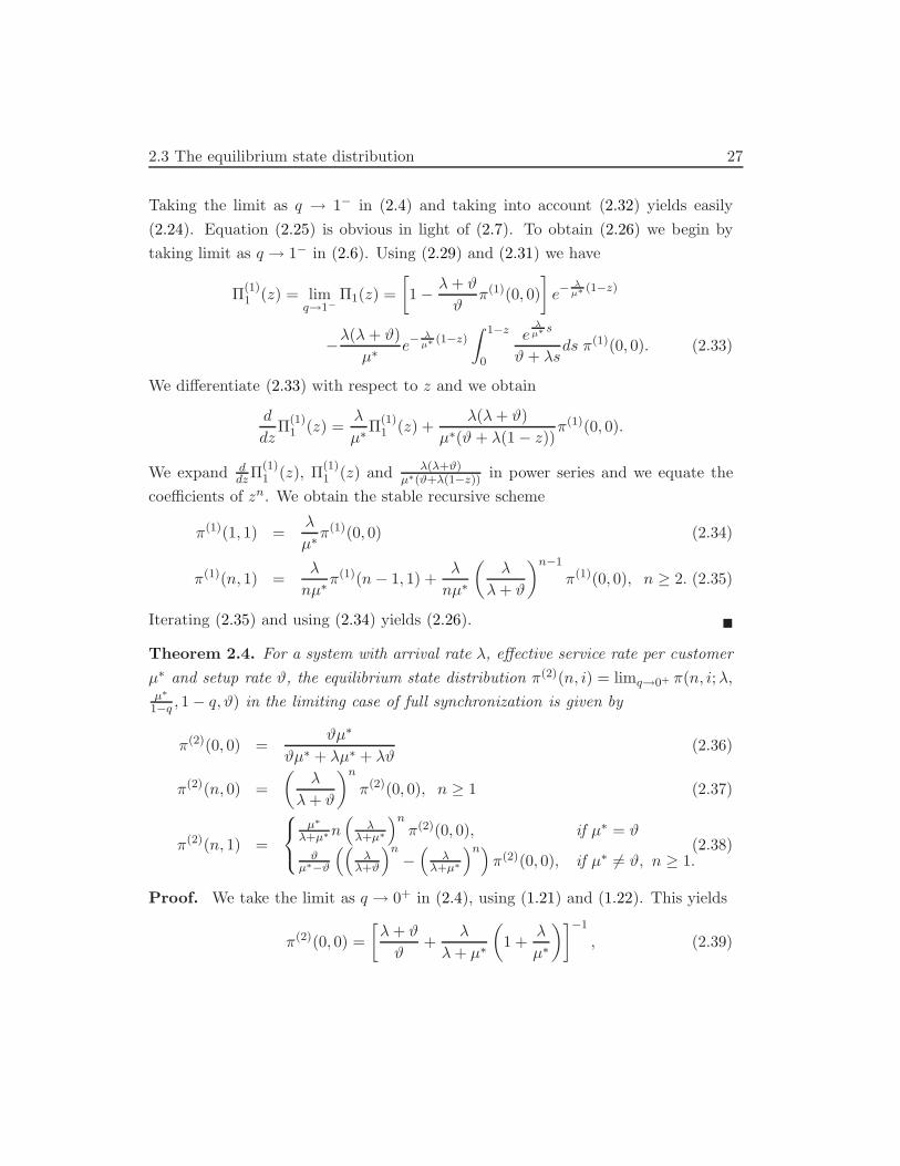
2.3 The equilibrium state distribution 27
Taking the limit as q " 1$ in (2.4) and taking into account (2.32) yields easily
(2.24). Equation (2.25) is obvious in light of (2.7). To obtain (2.26) we begin by
taking limit as q " 1$ in (2.6). Using (2.29) and (2.31) we have
#(1)1 (z) = lim
q%1!#1(z) =
0
1 !" + $
$%(1)(0, 0)
1
e$!
µ$ (1$z)
!"(" + $)
µ&e$
!µ$ (1$z)
+ 1$z
0
e!
µ$ s
$ + "sds %(1)(0, 0). (2.33)
We di"erentiate (2.33) with respect to z and we obtain
d
dz#(1)
1 (z) ="
µ&#(1)
1 (z) +"(" + $)
µ&($ + "(1 ! z))%(1)(0, 0).
We expand ddz#
(1)1 (z), #(1)
1 (z) and "("+#)µ$(#+"(1$z)) in power series and we equate the
coe!cients of zn. We obtain the stable recursive scheme
%(1)(1, 1) ="
µ&%(1)(0, 0) (2.34)
%(1)(n, 1) ="
nµ&%(1)(n ! 1, 1) +
"
nµ&
.
"
" + $
/n$1
%(1)(0, 0), n $ 2. (2.35)
Iterating (2.35) and using (2.34) yields (2.26). !
Theorem 2.4. For a system with arrival rate ", e!ective service rate per customer
µ& and setup rate $, the equilibrium state distribution %(2)(n, i) = limq%0+ %(n, i;",µ$
1$q , 1 ! q,$) in the limiting case of full synchronization is given by
%(2)(0, 0) =$µ&
$µ& + "µ& + "$(2.36)
%(2)(n, 0) =
.
"
" + $
/n
%(2)(0, 0), n $ 1 (2.37)
%(2)(n, 1) =
'
(
)
µ$
"+µ$ n2
""+µ$
3n%(2)(0, 0), if µ& = $
#µ$$#
22
""+#
3n!2
""+µ$
3n3
%(2)(0, 0), if µ& (= $, n $ 1..(2.38)
Proof. We take the limit as q " 0+ in (2.4), using (1.21) and (1.22). This yields
%(2)(0, 0) =
0
" + $
$+
"
" + µ&
.
1 +"
µ&
/1$1
, (2.39)
28 Synchronized services in a single server vacation queue
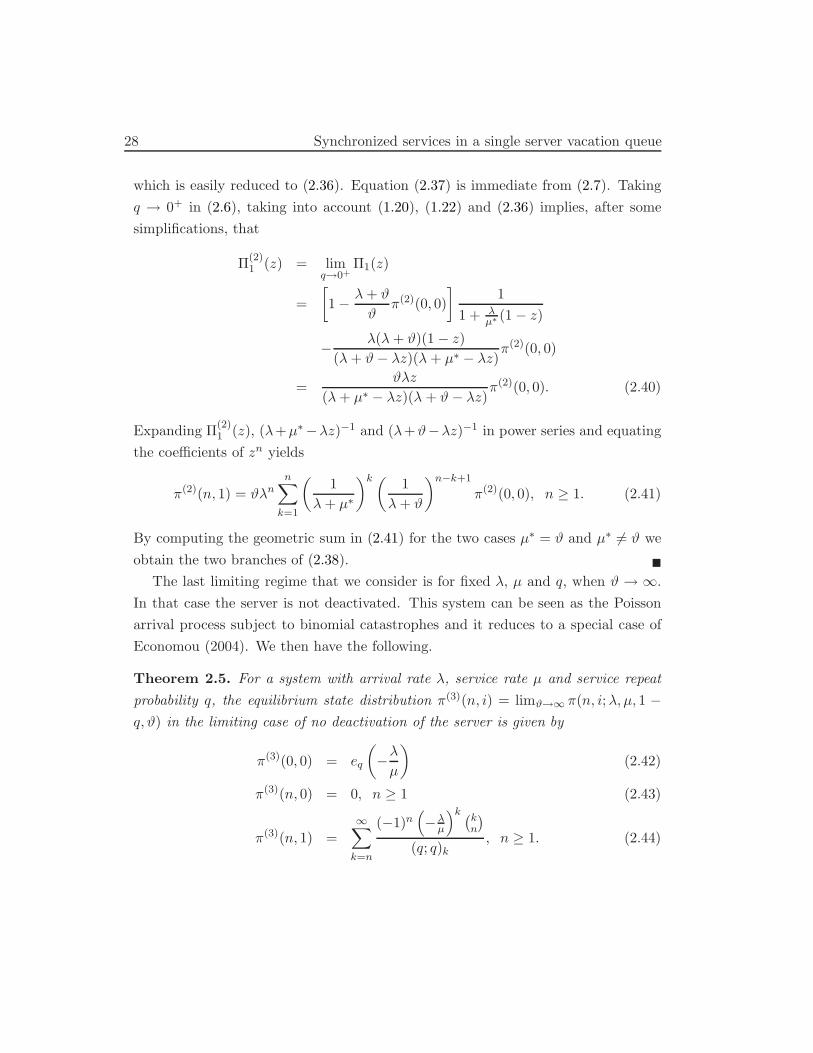
which is easily reduced to (2.36). Equation (2.37) is immediate from (2.7). Taking
q " 0+ in (2.6), taking into account (1.20), (1.22) and (2.36) implies, after some
simplifications, that
#(2)1 (z) = lim
q%0+#1(z)
=
0
1 !" + $
$%(2)(0, 0)
1
1
1 + "µ$ (1 ! z)
!"(" + $)(1 ! z)
(" + $! "z)(" + µ& ! "z)%(2)(0, 0)
=$"z
(" + µ& ! "z)(" + $! "z)%(2)(0, 0). (2.40)
Expanding #(2)1 (z), ("+µ&!"z)$1 and ("+$!"z)$1 in power series and equating
the coe!cients of zn yields
%(2)(n, 1) = $"nn$
k=1
.
1
" + µ&
/k . 1
" + $
/n$k+1
%(2)(0, 0), n $ 1. (2.41)
By computing the geometric sum in (2.41) for the two cases µ& = $ and µ& (= $ we
obtain the two branches of (2.38). !
The last limiting regime that we consider is for fixed ", µ and q, when $ " #.
In that case the server is not deactivated. This system can be seen as the Poisson
arrival process subject to binomial catastrophes and it reduces to a special case of
Economou (2004). We then have the following.
Theorem 2.5. For a system with arrival rate ", service rate µ and service repeat
probability q, the equilibrium state distribution %(3)(n, i) = lim#%# %(n, i;", µ, 1 !q,$) in the limiting case of no deactivation of the server is given by
%(3)(0, 0) = eq
.
!"
µ
/
(2.42)
%(3)(n, 0) = 0, n $ 1 (2.43)
%(3)(n, 1) =#$
k=n
(!1)n2
!"µ3k,kn
-
(q; q)k, n $ 1. (2.44)
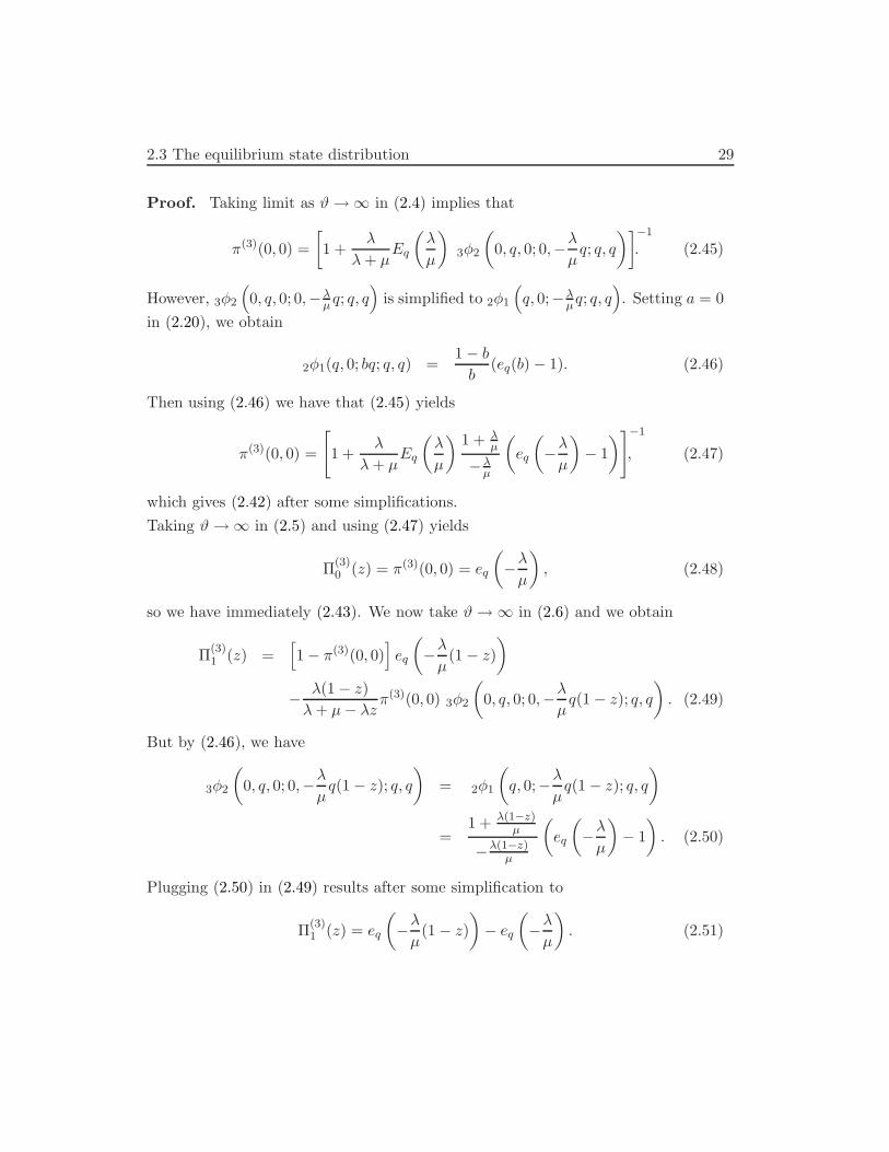
2.3 The equilibrium state distribution 29
Proof. Taking limit as $ " # in (2.4) implies that
%(3)(0, 0) =
0
1 +"
" + µEq
.
"
µ
/
3!2
.
0, q, 0; 0,!"
µq; q, q
/1$1
. (2.45)
However, 3!2
2
0, q, 0; 0,!"µ q; q, q3
is simplified to 2!1
2
q, 0;!"µq; q, q3
. Setting a = 0
in (2.20), we obtain
2!1(q, 0; bq; q, q) =1 ! b
b(eq(b) ! 1). (2.46)
Then using (2.46) we have that (2.45) yields
%(3)(0, 0) =
4
1 +"
" + µEq
.
"
µ
/
1 + "µ
!"µ
.
eq
.
!"
µ
/
! 1
/
5$1
, (2.47)
which gives (2.42) after some simplifications.
Taking $ " # in (2.5) and using (2.47) yields
#(3)0 (z) = %(3)(0, 0) = eq
.
!"
µ
/
, (2.48)
so we have immediately (2.43). We now take $ " # in (2.6) and we obtain
#(3)1 (z) =
%
1 ! %(3)(0, 0)&
eq
.
!"
µ(1 ! z)
/
!"(1 ! z)
" + µ ! "z%(3)(0, 0) 3!2
.
0, q, 0; 0,!"
µq(1 ! z); q, q
/
. (2.49)
But by (2.46), we have
3!2
.
0, q, 0; 0,!"
µq(1 ! z); q, q
/
= 2!1
.
q, 0;!"
µq(1 ! z); q, q
/
=1 + "(1$z)
µ
!"(1$z)µ
.
eq
.
!"
µ
/
! 1
/
. (2.50)
Plugging (2.50) in (2.49) results after some simplification to
#(3)1 (z) = eq
.
!"
µ(1 ! z)
/
! eq
.
!"
µ
/
. (2.51)
30 Synchronized services in a single server vacation queue
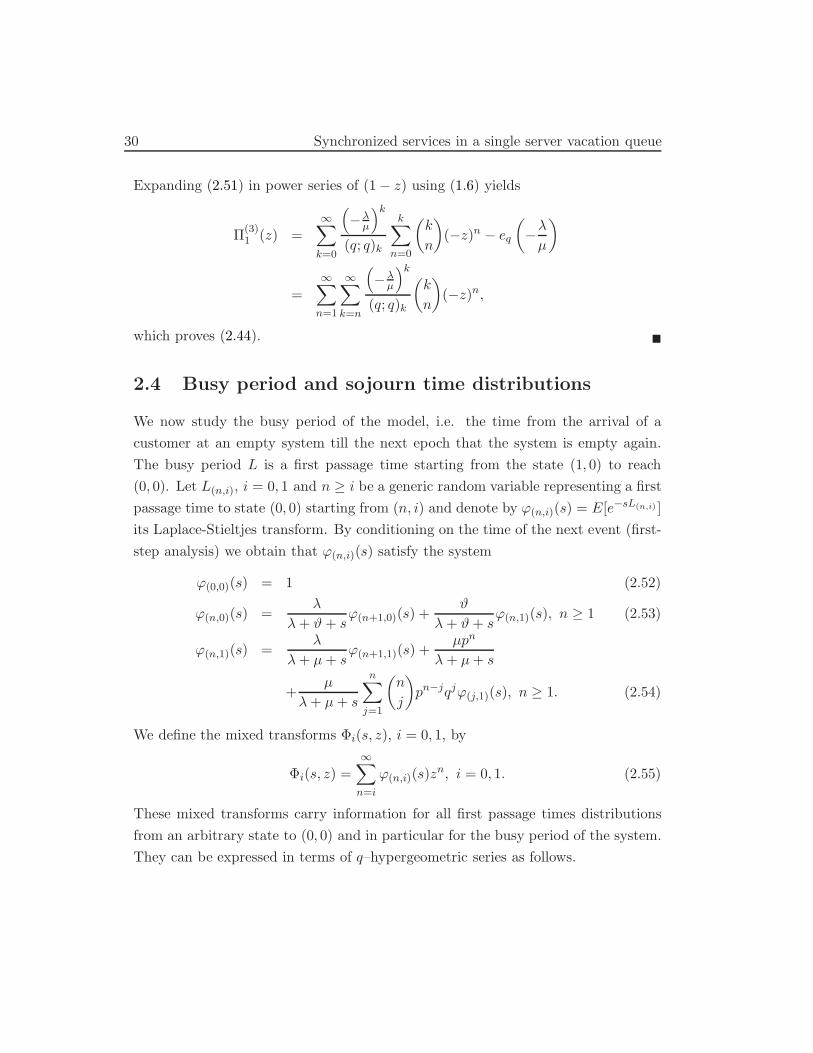
Expanding (2.51) in power series of (1 ! z) using (1.6) yields
#(3)1 (z) =
#$
k=0
2
!"µ3k
(q; q)k
k$
n=0
.
k
n
/
(!z)n ! eq
.
!"
µ
/
=#$
n=1
#$
k=n
2
!"µ3k
(q; q)k
.
k
n
/
(!z)n,
which proves (2.44). !
2.4 Busy period and sojourn time distributions
We now study the busy period of the model, i.e. the time from the arrival of a
customer at an empty system till the next epoch that the system is empty again.
The busy period L is a first passage time starting from the state (1, 0) to reach
(0, 0). Let L(n,i), i = 0, 1 and n $ i be a generic random variable representing a first
passage time to state (0, 0) starting from (n, i) and denote by &(n,i)(s) = E[e$sL(n,i) ]
its Laplace-Stieltjes transform. By conditioning on the time of the next event (first-
step analysis) we obtain that &(n,i)(s) satisfy the system
&(0,0)(s) = 1 (2.52)
&(n,0)(s) ="
" + $ + s&(n+1,0)(s) +
$
" + $ + s&(n,1)(s), n $ 1 (2.53)
&(n,1)(s) ="
" + µ + s&(n+1,1)(s) +
µpn
" + µ + s
+µ
" + µ + s
n$
j=1
.
n
j
/
pn$jqj&(j,1)(s), n $ 1. (2.54)
We define the mixed transforms $i(s, z), i = 0, 1, by
$i(s, z) =#$
n=i
&(n,i)(s)zn, i = 0, 1. (2.55)
These mixed transforms carry information for all first passage times distributions
from an arbitrary state to (0, 0) and in particular for the busy period of the system.
They can be expressed in terms of q–hypergeometric series as follows.
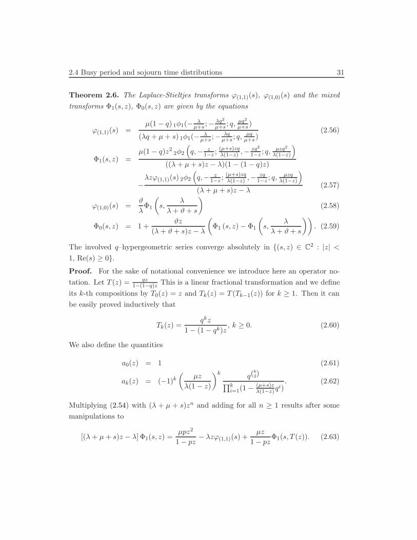
2.4 Busy period and sojourn time distributions 31
Theorem 2.6. The Laplace-Stieltjes transforms &(1,1)(s), &(1,0)(s) and the mixed
transforms $1(s, z), $0(s, z) are given by the equations
&(1,1)(s) =µ(1 ! q) 1!1(! "
µ+s ;!"q2
µ+s ; q,µq2
µ+s)
("q + µ + s) 1!1(! "µ+s ;!
"qµ+s ; q,
µqµ+s)
(2.56)
$1(s, z) =µ(1 ! q)z2
2!2
2
q,! z1$z ; (µ+s)zq
"(1$z) ,! zq2
1$z ; q, µzq2
"(1$z)
3
((" + µ + s)z ! ")(1 ! (1 ! q)z)
!"z&(1,1)(s) 2!2
2
q,! z1$z ; (µ+s)zq
"(1$z) ,! zq1$z ; q, µzq
"(1$z)
3
(" + µ + s)z ! "(2.57)
&(1,0)(s) =$
"$1
.
s,"
" + $ + s
/
(2.58)
$0(s, z) = 1 +$z
(" + $ + s)z ! "
.
$1 (s, z) ! $1
.
s,"
" + $ + s
//
. (2.59)
The involved q–hypergeometric series converge absolutely in {(s, z) % C2 : |z| <
1, Re(s) $ 0}.
Proof. For the sake of notational convenience we introduce here an operator no-
tation. Let T (z) = qz1$(1$q)z This is a linear fractional transformation and we define
its k-th compositions by T0(z) = z and Tk(z) = T (Tk$1(z)) for k $ 1. Then it can
be easily proved inductively that
Tk(z) =qkz
1 ! (1 ! qk)z, k $ 0. (2.60)
We also define the quantities
a0(z) = 1 (2.61)
ak(z) = (!1)k.
µz
"(1 ! z)
/k q(k2)
6ki=1(1 ! (µ+s)z
"(1$z)qi)
. (2.62)
Multiplying (2.54) with (" + µ + s)zn and adding for all n $ 1 results after some
manipulations to
[(" + µ + s)z ! "]$1(s, z) =µpz2
1 ! pz! "z&(1,1)(s) +
µz
1 ! pz$1(s, T (z)). (2.63)
32 Synchronized services in a single server vacation queue
By iterating (2.63) we obtain
[(" + µ + s)z ! "]$1(s, z) =µpz2
1 ! pz! "z&(1,1)(s)
+n$
k=1
4
k*
i=1
µTi(z)
q[(" + µ + s)Ti(z) ! "]
5
0
µpT 2k (z)
1 ! pTk(z)
1
!n$
k=1
4
k*
i=1
µTi(z)
q[(" + µ + s)Ti(z) ! "]
5
"Tk(z)&(1,1)(s)
+n+1*
i=1
µTi(z)
q[(" + µ + s)Ti(z) ! "][(" + µ + s)z ! "]$1(s, Tn+1(z)) (2.64)
and taking limits as the number of iterations n goes to infinity results similarly with
the derivation of (2.13) from (2.12) to
[(" + µ + s)z ! "]$1(s, z) =µpz2
1 ! pz! "z&(1,1)(s)
+#$
k=1
4
k*
i=1
µTi(z)
q[(" + µ + s)Ti(z) ! "]
5
0
µpT 2k (z)
1 ! pTk(z)
1
!#$
k=1
4
k*
i=1
µTi(z)
q[(" + µ + s)Ti(z) ! "]
5
"Tk(z)&(1,1)(s). (2.65)
The absolute convergence of the series can be proved straightforward by applying
the ratio test. We can now easily verify that
Ti(z)
(" + µ + s)Ti(s) ! "=
(!1)qiz
"(1 ! z)(1 ! (µ+s)z"(1$z)q
i), i $ 1
sok*
i=1
µTi(z)
q[(" + µ + s)Ti(s) ! "]= ak(z). (2.66)
We plug (2.66) into (2.65) and we obtain
[(" + µ + s)z ! "]$1(s, z) =#$
k=0
ak(z)
0
µpT 2k (z)
1 ! pTk(z)
1
!#$
k=0
ak(z)"Tk(z)&(1,1)(s). (2.67)
2.4 Busy period and sojourn time distributions 33
By setting z = ""+µ+s in equation (2.67) we obtain
&(1,1)(s) =
!#k=0 ak
2
""+µ+s
3
4
µpT 2k
“
!!+µ+s
”
1$pTk
“
!!+µ+s
”
5
!#k=0 ak
2
""+µ+s
3
"Tk
2
""+µ+s
3 . (2.68)
By writing the ratio of two consecutive terms of the sums in (2.68) as in (1.1), we
can express the sums in !-notation. Then (2.68) yields (2.56).
We then solve (2.67) for $1(s, z) and express the sums involved in the standard
manner to put them in !-notation. This yields (2.57).
We now multiply the equations (2.52) and (2.53) with z0 and zn respectively and
add for all n $ 0. After some algebraic manipulations we obtain that
[(" + $ + s)z ! "]$0(s, z) = (" + $ + s)z ! "! z"&(1,0)(s) + $z$1(s, z). (2.69)
We set z = ""+#+s in (2.69) and solve for &(1,0)(s) so we obtain (2.58). Solving (2.69)
for $0(s, z), taking into account (2.58) results in (2.59). !
We now consider a tagged customer and let S denote its sojourn time in the
system. The following theorem shows that the distribution of S is either a mixture
of exponential distributions with parameters µ(1 ! q) and $ (in the case where
µ(1!q) (= $) or a mixture of an exponential distribution and an Erlang-2 distribution
with parameter $ (in the case where µ(1 ! q) = $). More specifically we have the
following.
Theorem 2.7. The distribution of the sojourn time of a customer in the system is
given by
FS(x) =
7
(1 ! p1)(1 ! e$µ(1$q)x) + p1(1 ! e$#x), if $ (= µ(1 ! q)
(1 ! p2)(1 ! e$#x) + p2(1 ! e$#x ! xe$#x), if $ = µ(1 ! q), x $ 0,(2.70)
where
p1 =(" + $)µ(1 ! q)
$(µ(1 ! q) ! $)%(0, 0), p2 =
" + $
$%(0, 0). (2.71)
34 Synchronized services in a single server vacation queue
Proof. The sojourn time of a customer in the system depends on whether the
server is active or not at the time of his arrival. Because of the PASTA property
we have that the probability that the server is active at an arrival instant is #1(1)
given by (2.11) while the probability that the server is deactivated is #0(1). Then
the sojourn time S has the representation
S =
7
Y +!J
j=1 Xj , with probability "+## %(0, 0)
!Jj=1 Xj, with probability 1! "+#
# %(0, 0),(2.72)
where Y and X1,X2, . . . are independent exponentially distributed random variables
with rates $ and µ respectively and J is independent of them, representing the
number of services that will be required until the customer leaves the system. We
have that J is geometrically distributed with P (J = j) = (1 ! q)qj$1, j = 1, 2, . . ..
Because of (2.72) the Laplace-Stieltjes transform of S assumes the form
FS(s) =" + $
$%(0, 0)
$
$ + s
µ(1 ! q)
µ(1 ! q) + s+
.
1 !" + $
$%(0, 0)
/
µ(1 ! q)
µ(1 ! q) + s. (2.73)
The partial fraction expansion of (2.73) yields
FS(s) =
'
(
)
(1 ! p1)µ(1$q)
µ(1$q)+s + p1##+s , if $ (= µ(1 ! q)
(1 ! p2)##+s + p2
2
##+s
32, if $ = µ(1 ! q)
where p1, p2 are given by (2.71) and we invert to obtain (2.70). !
2.5 Numerical results
In this section we present some numerical results that shed further light in the be-
havior of the model. We begin by illustrating the e"ect of each single parameter
p, $ and " in the mean number of customers in the system, E[N ], when the other
parameters are kept fixed. In all numerical scenarios we assume that the time unit
has been re-scaled to agree with the mean service time, i.e. we set µ = 1. Our results
are based on the computation of the mean number of customers given from equation
(2.18) of theorem 2.2. In figure 2.2 we present the graph of E[N ] with respect to p
for " = 3.5 and $ = 1.5. The function is decreasing convex as p varies from 0 to 1.

2.5 Numerical results 35
0 0.2 0 .4 0 .6 0 .8 10
5
10
15
20
25
30
35
40
45
50
p
E[N
;p]
λ=3.5
θ=1.5
µ=1
Fig. 2.2: E[N ;", µ, p,$] versus p.
0 2 4 6 8 10 123.5
3 .55
3.6
3 .65
3.7
3 .75
3.8
θ
E[N
;θ]
λ=3.5
µ=1
p=0.5
Fig. 2.3: E[N ;", µ, p,$] versus $.
0 0.5 1 1.5 20
0.2
0 .4
0 .6
0 .8
1
1.2
1 .4
1 .6
1 .8
2
λ
E[N
;λ]
θ=1.5
µ=1
p=0.5
Fig. 2.4: E[N ;", µ, p,$] versus ".
Figure 2.3 shows the influence of the setup rate $ in the mean number of customers
in the system, when " = 3.5 and p = 0.5. The function is decreasing convex with
a horizontal asymptote as $ " #. This agrees with our intuitive expectation and
the result of theorem 2.5. Figure 2.4 shows the behavior of E[N ] as the arrival rate
" varies, when $ = 1.5 and p = 0.5. As expected, the mean number of customers in
the system increases when " increases.
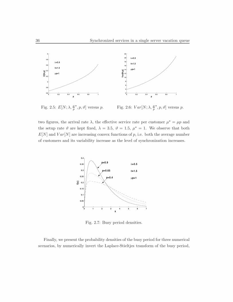
The next figures 2.5 and 2.6 demonstrate the e"ect of the level of synchronization
in the mean and the variance of the number of customers in the system. In these
36 Synchronized services in a single server vacation queue
0 0.2 0 .4 0 .6 0 .8 13.6
3 .8
4
4.2
4 .4
4 .6
4 .8
5
p
E[N
;p]
λ=3.5
θ=1.5
µp=1
Fig. 2.5: E[N ;", µp$, p,$] versus p.
0 0.2 0 .4 0 .6 0 .8 12
4
6
8
10
12
14
16
18
20
22
p
Var
[N;p
]
λ=3.5
θ=1.5
µp=1
Fig. 2.6: V ar[N ;", µp$, p,$] versus p.
two figures, the arrival rate ", the e"ective service rate per customer µ$ = µp and
the setup rate $ are kept fixed, " = 3.5, $ = 1.5, µ$ = 1. We observe that both
E[N ] and V ar[N ] are increasing convex functions of p, i.e. both the average number
of customers and its variability increase as the level of synchronization increases.
0 1 2 3 4 5 6 70
0.05
0.1
0 .15
0.2
0 .25
0.3
0 .35
0.4
x
f(x)
λ=3.5
θ=1.5
µp=1
p=0.9
p=0.65
p=0.4
Fig. 2.7: Busy period densities.
Finally, we present the probability densities of the busy period for three numerical
scenarios, by numerically invert the Laplace-Stieltjes transform of the busy period,
2.5 Numerical results 37
&(1,0)(s), given in theorem 2.6. Although there is no symbolic inversion of &(1,0)(s),
the use of the r!s notation enables us to compute the numerical inversion very easily,
by exploiting the available procedures and algorithms that support the computation
of q–hypergeometric series in all standard mathematical software packages. In these
scenarios we assume that " = 3.5, $ = 1.5, µp = 1 and we consider three cases
for p: 0.4, 0.65 and 0.9. Again, the numerical findings in figure 2.7 are in absolute
accordance with the fact that the mean number of customers increases as the level
of synchronization increases.

38 Synchronized services in a single server vacation queue
Chapter 3
Synchronized abandonments in
a single server unreliable
queue
We consider a single server unreliable queue represented by a 2-dimensional contin-
uous time Markov chain. At failure times, all present customers leave the system.
Moreover, customers become impatient and perform synchronized abandonments, as
long as the server is down. We analyze this model and derive the main performance
measures using results from the basic q–hypergeometric series.
3.1 Introduction
In the queueing literature, there exists a significant number of papers dealing with
queueing systems with abandonments. In the majority of the papers, the source
of the impatience has been taken to be either a long wait already experienced at a
queue, or a long wait anticipated by the customers. Recently, Altman and Yechiali
(2006, 2008), Perel and Yechiali (2009) and Yechiali (2007) considered systems with
server(s) alternating between on and o" periods, where customers’ impatience is due
to the absence of the server(s). Such systems can model satisfactorily the reneging
40 Synchronized abandonments in a single server unreliable queue
behavior of waiting customers in real systems with servers that are temporarily un-
available due to either scheduled vacations or failures.
Models with servers alternating between on and o" periods and customers’ aban-
donments are generally hard to analyze. In a Markovian framework, the state of
such a system is typically represented by a vector (n, i), where n records the num-
ber of customers and i the state of the server(s). However, the abandonments that
the customers perform independently lead to transitions out of a state (n, 0) to a
state (n ! 1, 0) with rates proportional to n. In this sense, the independent aban-
donments of the customers give rise to ‘spatially inhomogeneous’ continuous time
Markov chains. This is also the distinctive feature in queueing models with an in-
finite number of servers, retrial queueing models and population growth models in
Mathematical Biology, since every individual is associated with births and deaths.
In most cases these models are mathematically intractable and it is not possible to
conclude with closed form results.
There are only a few research works trying to extend matrix analytic methods or
other analytic tools for models with this type of spatial inhomogeneity. In general,
the authors use truncation or generalized truncation ideas to study the systems (see
e.g. Artalejo and Pozo (2002) and the references therein) or they apply generating
function methods. However, we have to note that in this case the partial generating
functions of the number of individuals in system satisfy a system of linear di"erential
equations in contrast with the ‘spatially homogeneous’ case where they satisfy linear
algebraic equations. Such systems are usually intractable or can be solved in terms
of hypergeometric series (see e.g. Altman and Yechiali (2006, 2008), Artalejo and
Gomez-Corral (1997), Baykal-Gursoy and Xiao (2004), Keilson and Servi (1993),
Krishnamoorthy et al. (2005), Perel and Yechiali (2009) and Yechiali (2007)).
The aim of this chapter is to extend the study of queues with disasters and im-
patient customers when the system is down that was introduced by Yechiali (2007).
Yechiali (2007) considered Markovian queues subject to disasters that remove all
the customers from the system and turn the server down. As long as the server is
3.1 Introduction 41
down, he assumed that the arrivals continue to come, but the customers become
impatient and perform independent abandonments, that is, every customer sets on
his own exponential patience clock and leaves the system when his patience time
expires. We assume that the customers are impatient but they perform synchronized
abandonments. Such a model is motivated by remote systems where customers have
to wait for a certain transport facility to abandon the system. Then, whenever the
facility visits the system, the present customers can decide whether to leave the sys-
tem or not. Therefore, we have synchronized departures for some of the customers.
More specifically, we assume that the abandonment opportunities occur according
to a Poisson process at rate ', whenever the server is down (so we can think that the
transportation facility’s arrivals occur according to this process). Then, at an aban-
donment opportunity epoch, every customer decides to abandon the system with
probability p or remains in the system waiting for service with probability q = 1!p,
independently of the others. This implies that there exist binomial transition rates
of the form ',nn#
-
pn$n#qn#
, from a state (n, 0) to states (n", 0), for 0 & n" & n. Similar
Markov chains occur in Mathematical Biology in the study of population processes
subject to binomial catastrophes (see e.g. Artalejo et al. (2007), Brockwell et al.
(1982), Economou (2004) and Economou and Fakinos (2008)). Moreover, Neuts
(1994) studied a 1-dimensional discrete-time model with similar dynamics.
We show that the framework of basic q–hypergeometric series enables us to ex-
press in closed form the main performance measures of this system. In general, the
theory of q–hypergeometric series can facilitate the computations regarding systems
with this kind of binomial transitions arising from synchronization.
The chapter is organized as follows. In section 3.2 we describe the model and
introduce the appropriate notation. In section 3.3 we carry out the equilibrium anal-
ysis of the system state and derive several exact formulas and iterative algorithmic
schemes. Some limiting regimes with a particular interest are discussed in more
detail. In section 3.4 we study the sojourn time of a customer, while in section 3.5
we treat the system busy period distribution of the model.
42 Synchronized abandonments in a single server unreliable queue
3.2 Model description and notation
We consider an M/M/1 queueing system in which customers arrive according to a
Poisson process at rate ". The service is provided by a single server, who serves the
customers on a FCFS basis. The successive service times are independent exponen-
tially distributed random variables with rate µ. The system is subject to failures
that occur when the server is at a functioning state, according to a Poisson process
at rate (. At a failure epoch, the server is turned o" and all present customers are
forced to leave the system. Then, the repair process starts immediately. The repair
times are exponentially distributed random variables with rate ). While the server
is o", the stream of new arrivals continues. However, since the server is down, these
new customers become impatient and perform synchronized abandonments in the
following way: A transportation facility is set on and it arrives at the system accord-
ing to a Poisson process at rate '. Every arrival epoch of the transportation facility
constitutes an abandonment opportunity for the present customers. We suppose
that each one of them decides to abandon the system with probability p or remains
in the system with probability q, independently of the others.
The system is represented by a continuous-time Markov chain {(N(t), I(t)) : t $0}, where N(t) is the number of customers in the system at time t and I(t) denotes
the state of the server at time t (0=o" (under repair) and 1=on (functioning)), t $ 0.
The corresponding transition rate diagram is given in figure 3.1.
Let (%(n, i) : n $ 0 and i = 0, 1) denote the equilibrium distribution of
{(N(t), I(t))}. We also define the partial probability generating functions #0(z)
and #1(z) by
#0(z) =#$
n=0
%(n, 0)zn and #1(z) =#$
n=0
%(n, 1)zn .
In section 3.3 we will determine #0(z) and #1(z) in terms of q–hypergeometric
series. Moreover, in sections 3.4 and 3.5 we will also see that the study of the sojourn
times and the busy period distribution of this system is also facilitated using the
theory of q–hypergeometric series.
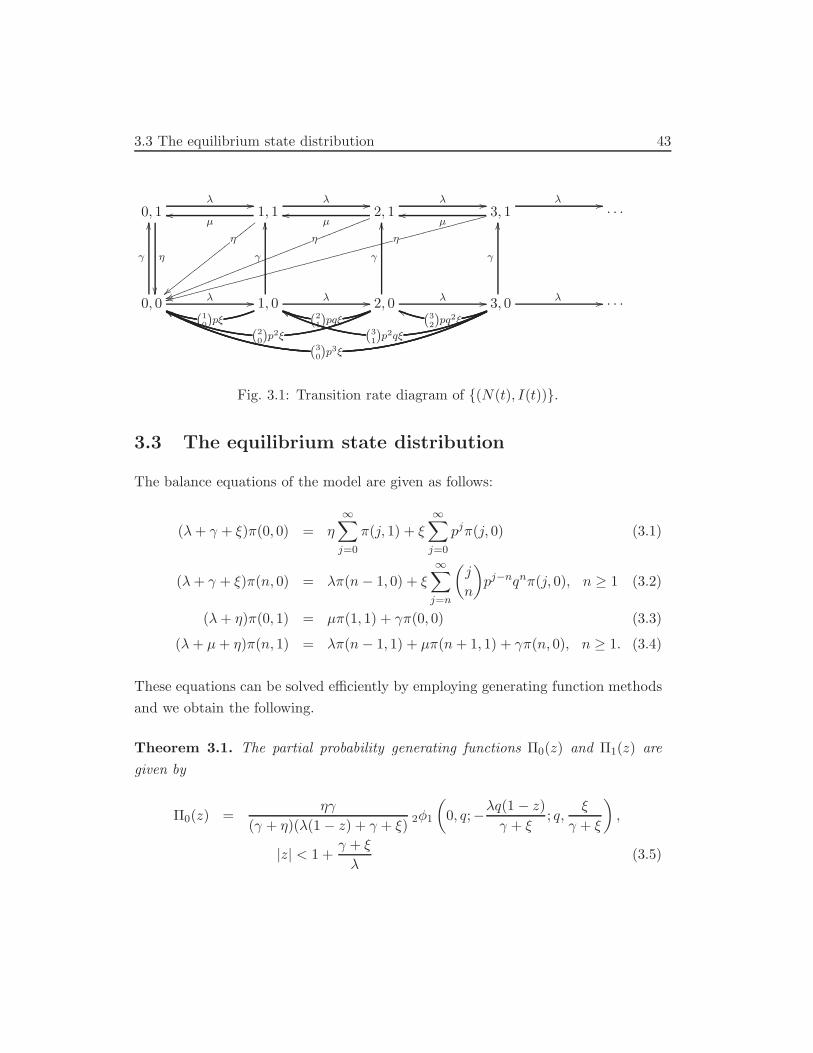
3.3 The equilibrium state distribution 43
0, 1" ##
%
..
1, 1
%!!!
!
//!!!!!!!
!!!!!!
µ00
" ##2, 1
%"""""""""
11""""""""""""""""""""""""
" ##
µ00 3, 1
%##############
22####################################
" ##
µ00 · · ·
0, 0
&
--
" ## 1, 0
&
--
(10)p'
""" ## 2, 0
&
--
(21)pq'
""
(20)p
2'
33" ## 3, 0
&
--
(32)pq2'
""
(31)p
2q'
33
(30)p3'
33" ## · · ·
Fig. 3.1: Transition rate diagram of {(N(t), I(t))}.
3.3 The equilibrium state distribution
The balance equations of the model are given as follows:
(" + ) + ')%(0, 0) = (#$
j=0
%(j, 1) + '#$
j=0
pj%(j, 0) (3.1)
(" + ) + ')%(n, 0) = "%(n ! 1, 0) + '#$
j=n
.
j
n
/
pj$nqn%(j, 0), n $ 1 (3.2)
(" + ()%(0, 1) = µ%(1, 1) + )%(0, 0) (3.3)
(" + µ + ()%(n, 1) = "%(n ! 1, 1) + µ%(n + 1, 1) + )%(n, 0), n $ 1. (3.4)
These equations can be solved e!ciently by employing generating function methods
and we obtain the following.
Theorem 3.1. The partial probability generating functions #0(z) and #1(z) are
given by
#0(z) =()
() + ()("(1 ! z) + ) + ')2!1
.
0, q;!"q(1 ! z)
) + '; q,
'
) + '
/
,
|z| < 1 +) + '
"(3.5)
44 Synchronized abandonments in a single server unreliable queue
#1(z) =)(1 ! z0)z#0(z) ! )(1 ! z)z0#0(z0)
((" + µ + ()z ! "z2 ! µ)(1 ! z0),
|z| < min
.
1 +) + '
", z1
/
, (3.6)
where
z0 =" + µ + ( !
8
(" + µ + ()2 ! 4"µ
2"% (0, 1), (3.7)
z1 =" + µ + ( +
8
(" + µ + ()2 ! 4"µ
2"% (1,#). (3.8)
The convergence of the series is absolute in the corresponding open disks and uniform
in every compact subset of them.
Proof. Summing equations (3.1) and (3.2) over all n = 0, 1, . . . we obtain that
)#0(1) = (#1(1). (3.9)
Equation (3.9) together with the normalization equation #0(1) + #1(1) = 1 yields
that
#0(1) =(
) + (, #1(1) =
)
) + (. (3.10)
Multiplying equations (3.1) and (3.2) by z0 and zn respectively and summing for all
n = 0, 1, . . ., we obtain that
(" + ) + ')#0(z) = "z#0(z) + '#$
n=0
#$
j=n
.
j
n
/
pj$nqn%(j, 0)zn + (#$
j=0
%(j, 1)
= "z#0(z) + '#$
j=0
%(j, 0)(p + qz)j + (#1(1)
= "z#0(z) + '#0(p + qz) + (#1(1).
Hence
#0(z) ='
"(1 ! z) + ) + '#0(1 ! q + qz) +
(#1(1)
"(1 ! z) + ) + '. (3.11)
3.3 The equilibrium state distribution 45
Iterating equation (3.11) yields
#0(z) = #0(1 ! qn+1 + qn+1z)n*
i=0
'
"qi(1 ! z) + ) + '
+(#1(1)n$
k=0
1
"qk(1 ! z) + ) + '
k$1*
i=0
'
"qi(1 ! z) + ) + ', (3.12)
where we assume that for k = 0 the empty product6k$1
i=0 is by definition equal to
1. Taking the limit as n " # in (3.12) we obtain
#0(z) = (#1(1)#$
k=0
1
"qk(1 ! z) + ) + '
k$1*
i=0
'
"qi(1 ! z) + ) + ', (3.13)
whenever the series converges.
Expressing equation (3.13) in terms of the canonical form of q–series we obtain that
#0(z) =(
"(1 ! z) + ) + '#1(1) 2!1
.
0, q;!"q(1 ! z)
) + '; q,
'
) + '
/
. (3.14)
Then by substituting #1(1) from (3.10) yields equation (3.5). The absolute conver-
gence of the series (3.5) is guaranteed for z % {z % C : |z| < 1 + &+'" }. Indeed,
we first observe that the 2!1
2
0, q;!"q(1$z)&+' ; q, '
&+'
3
series converges absolutely (see
the comments after the definition (1.2)) for all z such that !"q(1$z)&+' (= q$m, for
m = 0, 1, 2, . . ., consequently it converges for z with |z| < 1 + &+'"q . Moreover, the
denominator in (3.5) does not vanish for z (= 1 + &+'" . Hence the partial probability
generating function #0(z) as given in equation (3.5) converges for |z| < 1 + &+'" .
Multiplying equations (3.3) and (3.4) by z0 and zn respectively and summing for
all n = 0, 1, . . . we obtain
(" + µ + ()#1(z) ! µ%(0, 1) = "z#1(z) +µ
z(#1(z) ! %(0, 1)) + )#0(z),
or equivalently
((" + µ + ()z ! "z2 ! µ)#1(z) = !µ(1 ! z)%(0, 1) + )z#0(z). (3.15)
46 Synchronized abandonments in a single server unreliable queue
Equation (3.15) is identical to Yechiali (2007) equation (2.6). We observe that the
quadratic polynomial
f(z) = (" + µ + ()z ! "z2 ! µ (3.16)
has two real roots z0 and z1 given by (3.7) and (3.8). Setting z = z0 in equation
(3.15) (note that #1(z0) converges since z0 < 1) yields
%(0, 1) =)z0#0(z0)
µ(1 ! z0). (3.17)
Substituting (3.17) into (3.15) and solving for #1(z) yields (3.6). Having established
the radius of convergence for #0(z), it can be easily checked that the partial prob-
ability generating function #1(z) given by (3.6) converges for z % {z % C : |z| <
min(1 + &+'" , z1)}. !
We can now use (3.5)-(3.6) to derive explicit expressions for some important
performance measures of the system. More specifically, we will derive the factorial
moments of the number of customers in the system and the stationary probabilities
in some limiting regimes.
We can now proceed to the calculation of the moments for the distribution of
the number of customers in the system. Note that the moments of all orders exist
since the partial probability generating functions #0(z) and #1(z) converge inside
an open disk with radius of convergence strictly greater than 1.
Remark 3.1. Di!erentiating (3.11) n times and setting z = 1 yields
#(n)0 (1) =
n"
) + '(1 ! qn)#(n$1)
0 (1), n $ 1. (3.18)
Di!erentiating (3.15) n times and setting z = 1 yields
)#(1)0 (1) + )#(0)
0 (1) + µ%(0, 1) = (#(1)1 (1) + (µ + ( ! ")#(0)
1 (1)
)#(n)0 (1) + n)#(n$1)
0 (1) = (#(n)1 (1) + n(µ + ( ! ")#(n$1)
1 (1)
!n(n ! 1)"#(n$2)1 (1), n $ 2. (3.19)
3.3 The equilibrium state distribution 47
Equations (3.18) and (3.19) form an iterative scheme with initial conditions for
#(0)0 (1) = #0(1) and #(0)
1 (1) = #1(1) given by (3.10). The first order scheme given
by (3.18) gives easily #(n)0 (1) in product closed form for any desired n. However, the
second order scheme given by (3.19) has coe"cients and constant term that depend
on n, so its direct solution seems impossible. Nevertheless, a closed form for #(n)1 (1)
can be obtained by applying results from the theory of q–series, in particular using
Heine’s transformation formulas (1.11)-(1.13).
We have the following theorem.
Theorem 3.2. The factorial moments m(n) = E[N(N ! 1)(N ! 2) · · · (N ! n + 1)]
of the equilibrium number of customers in the system are given by
m(n) =)
) + (
n!
z1 ! z0
n$
k=0
"n
(k6n$k
i=1 () + '(1 ! qi))
%
z1(1 ! z0)k+1 ! z0(1 ! z1)
k+1&
+)z0#0(z0)
1 ! z0
n!("/()n$1
((z1 ! z0)[(1 ! z0)
n ! (1 ! z1)n]
+(
) + (
n!"n
6ni=1() + '(1 ! qi))
, n $ 1, (3.20)
where z0 and z1 are given in equations (3.7) and (3.8) respectively. In particular
E[N ] =)
(
z0#0(z0)
1 ! z0+
)
) + (
"! µ
(+
"
) + '(1 ! q). (3.21)
Proof. The factorial moments exponential generating function P (z) is given by
P (z) =#$
n=0
m(n)zn
n!= E
4
#$
n=0
.
N
n
/
zn
5
= E[(1+z)N ] = #0(1+z)+#1(1+z). (3.22)
We have already shown in theorem 3.1 that #0(z) and #1(z) converge in a neigh-
borhood of 1, hence P (z) is well defined in a neighborhood of 0. Using Heine’s
transformation formula (1.12), equation (3.5) assumes the form
#0(z) =(
) + ( 2!1
.
0, q;'q
) + '; q,!
"(1 ! z)
) + '
/
=(
) + (
#$
n=0
"n
6ni=1() + '(1 ! qi))
(z ! 1)n,
48 Synchronized abandonments in a single server unreliable queue
that gives
#0(1 + z) =(
) + (
#$
n=0
"n
6ni=1() + '(1 ! qi))
zn. (3.23)
Moreover from equation (3.6) we obtain that
#1(1 + z) = )(1 + z)#0(1 + z)
f(1 + z)+ )
z0#0(z0)
1 ! z0
z
f(1 + z), (3.24)
where f(z) = !"(z0 ! z)(z1 ! z) is given in equation (3.16). By partial fraction
expansion and elementary algebra we obtain that
1
f(1 + z)=
1
"(z1 ! z0)(1 ! z0)
1
1 + z1$z0
+1
"(z1 ! z0)(z1 ! 1)
1
1 ! zz1$1
=#$
n=0
1
"(z1 ! z0)
0
(!1)n
(1 ! z0)n+1+
1
(z1 ! 1)n+1
1
zn
=#$
n=0
("/()n
((z1 ! z0)
9
(!1)n(z1 ! 1)n+1 + (1 ! z0)n+1:
zn, (3.25)
and then easily
1 + z
f(1 + z)=
#$
n=0
("/()n
((z1 ! z0)
9
(!1)nz0(z1 ! 1)n+1 + z1(1 ! z0)n+1:
zn. (3.26)
Now (3.23) and (3.26) imply easily that
(1 + z)#0(1 + z)
f(1 + z)=
1
() + ()(z1 ! z0)
#$
n=0
n$
k=0
"n
(k6n$k
i=1 () + '(1 ! qi))
)%
(!1)kz0(z1 ! 1)k+1 + z1(1 ! z0)k+1&
zn , (3.27)
where z0 and z1 are given in equations (3.7) and (3.8), respectively. Plugging (3.25)
and (3.27) into (3.24) and using (3.23), we can expand (3.22) in powers of z. After
some straightforward algebra we obtain (3.20) and in particular, for n = 1, we de-
duce (3.21). !
In the model we have two types of lost customers, those that abandon the system
due to impatience during the repair phase of the server and those that are forced
3.3 The equilibrium state distribution 49
to leave the system at the failure epochs of the server. We will now calculate the
proportion of customers who leave the system at the failure epochs, the proportion
of customers who abandon the system because of impatience and the proportion of
served customers. We begin by computing the corresponding rates.
When the system is in state (n, 1), n $ 0, the failure rate of the server is ( and
when a failure occurs all present customers leave the system, therefore the rate of
lost customers due to failures, Rfailures, is given by
Rfailures =#$
n=0
(n%(n, 1) = (#"1(1). (3.28)
Similarly, the rate of served customers, Rserved, is given by
Rserved =#$
n=1
µ%(n, 1) = µ(#1(1) ! %(0, 1)). (3.29)
Finally, the rate of abandonments due to impatience when the server is down,
Rabandonments, is given by
Rabandonments = "! Rfailures ! Rserved = '(1 ! q)#"0(1). (3.30)
Clearly, #"0(1) can be directly obtained from equation (3.18), that is #"
0(1) =%&+%
"&+'(1$q) , while #"
1(1) can be obtained as #"1(1) = E[N ] ! #"
0(1) = &z0!0(z0)%(1$z0) +
"$µ%
&&+% + &
&+%"
&+'(1$q) , since the mean number of customers in the system, E[N ], is
given in equation (3.21). The fractions of lost customers due to failures, served cus-
tomers and lost customers due to abandonments are readily computed by dividing
(3.28)-(3.30) by the overall rate ".
We now turn our attention to the behavior of the model under certain limiting
regimes. To emphasize the dependence on the parameters of the model in the rest
of this section, we will denote %(n, i), #0(z) and #1(z) by %(n, i;", µ, ', p, ), (),
#0(z;", µ, ', p, ), () and #1(z;", µ, ', p, ), (), respectively. Note that 'p can be
thought of as the e"ective abandonment rate per customer. Indeed the overall
abandonment time of a customer is a geometric sum of exponentially distributed
50 Synchronized abandonments in a single server unreliable queue
random variables with rate ' and so we can easily see that it is also exponentially
distributed with parameter 'p. Under this perspective, if we have two models with
the same parameters ", µ, ) and ( that di"er only in ' and p, but with 'p = '& fixed,
we can think that the models have identical arrival rates ", service rates µ, e"ec-
tive abandonment rates per customer '&, setup rates ) and catastrophe rates ( and
di"er only in the ‘level of synchronization’ p. Indeed, the case p " 0+ corresponds
to no synchronization since the customers depart almost singly at the abandonment
epochs. On the contrary, the case p " 1$ corresponds to full synchronization since
almost all present customers depart simultaneously from the system when an aban-
donment opportunity occurs.
We are interested in studying the equilibrium behavior of the system for the case
where ", µ, '&, ) and ( are kept fixed in the two limiting cases p " 0+ (q " 1$)
and p " 1$ (q " 0+). The case p " 0+ corresponds exactly to the model studied
by Yechiali (2007) where the customers perform independent abandonments. In
theorem 3.3 we derive the equilibrium state probability generating functions while
in theorem 3.4 we obtain the factorial moments of the state distribution.
Theorem 3.3. For a system with arrival rate ", service rate µ, e!ective aban-
donment rate per customer '&, setup rate ) and catastrophe rate (, the generating
functions
#(1)i (z) = lim
q%1!#i(n, i;", µ,
'&
1 ! q, 1 ! q, ), (), i = 0, 1,
in the limiting case of no synchronization are given by
#(1)0 (z) =
()
( + )
1
'&
+ 1
z
(1 ! t)"#$$1
(1 ! z)"#$
e$!#$
(t$z)dt (3.31)
#(1)1 (z) =
)(1 ! z0)z#(1)0 (z) ! )(1 ! z)z0#
(1)0 (z0)
((" + µ + ()z ! "z2 ! µ)(1 ! z0), (3.32)
where z0 ="+µ+%$
*("+µ+%)2$4"µ2" .
Proof. Using Heine’s transformation formula (1.11), equation (3.5) assumes the
3.3 The equilibrium state distribution 51
following form
#0(z) =(
) + (
)
) + '
(q; q)#
(!"(1$z)&+' , '
&+' ; q)#2!1
.
!"(1 ! z)
) + ',
'
) + '; 0; q, q
/
.
(3.33)
We use (1.19) and we obtain that
(1 ! q) 2!1
.
!"(1 ! z)
) + ',
'
) + '; 0; q, q
/
=(!"(1$z)
&+' , '&+' ; q)#
(q; q)#
+ 1
0
(qt; q)#
(!"(1$z)t&+' , 't&+' ; q)#
dqt. (3.34)
Plugging (3.34) into (3.33) and simplifying several terms we have that (3.33) assumes
the form
#0(z) =(
) + (
)
)(1 ! q) + '&
+ 1
0
(qt; q)#
(!"(1$z)t&+' , 't&+' ; q)#
dqt
=(
) + (
)
)(1 ! q) + '&
+ 1
0
(qt; q)#
( 't&+' ; q)#eq(!
"(1 ! z)t
) + ')dqt. (3.35)
Replacing ' by '$
1$q and using (1.8) and (1.10) we have
limq%1!
eq
.
!"(1 ! z)t
) + '
/
= limq%1! eq
2
! "(1$z)t&(1$q)+'$ (1 ! q)
3
= e$!#$ (1$z)t. (3.36)
limq%1!
(qt; q)#
( 't&+' ; q)#= limq%1!
(q(1+ "(1!q)#$ ) #$t
"(1!q)+#$ ;q)"
( #$t"(1!q)+#$ ;q)"
= (1 ! t)"#$ $1. (3.37)
Taking the limit as q " 1$ in (3.35), taking into account equations (3.36) and (3.37)
and setting t = s$z1$z yields (3.31), which is Yechiali (2007) formula (2.7). Equation
(3.32) results immediately from (3.6). !
Theorem 3.4. The factorial moments m(1)(n) = E[N(N ! 1)(N ! 2) · · · (N ! n + 1)]
52 Synchronized abandonments in a single server unreliable queue
of the equilibrium number of customers in the system are given by
m(1)(n) =
)
) + (
n!
z1 ! z0
n$
k=0
"n
(k6n$k
i=1 () + '&i)
%
z1(1 ! z0)k+1 ! z0(1 ! z1)
k+1&
+)z0#
(1)0 (z0)
1 ! z0
n!("/()n$1
((z1 ! z0)[(1 ! z0)
n ! (1 ! z1)n]
+(
) + (
n!"n
6ni=1() + '&i)
, n $ 1, (3.38)
where z0 and z1 are given in equations (3.7) and (3.8) respectively and #(1)0 (z0) is
given by (3.31). In particular
E(1)[N ] =)
(
z0#(1)0 (z0)
1 ! z0+
)
) + (
"! µ
(+
"
) + '&. (3.39)
Proof. We replace ' by '&/(1 ! q) in (3.20) and (3.21) and we take the limit as
q " 1$. We obtain (3.38) and (3.39) respectively. !
The expression (3.39) gives the mean number of customers in Yechiali (2007)
model. Indeed, Yechiali (2007) equations (2.10) and (2.13) can be used to derive
independently our equation (3.39).
We now derive the corresponding results for the other extreme case of full syn-
chronization, i.e. when p " 1$. In theorem 3.5 we derive the equilibrium state
probability generating functions while in theorem 3.6 we obtain the factorial mo-
ments of the state distribution.
Theorem 3.5. For a system with arrival rate ", service rate µ, e!ective abandon-
ment rate per customer '&, setup rate ) and catastrophe rate (, the equilibrium state
distribution %(2)(n, i) = limq%0+ %(n, i;", µ, '$
1$q , 1 ! q, ), () in the limiting case of
full synchronization is given by
%(2)(n, 0) = c1
.
"
) + '& + "
/n
, n $ 0 (3.40)
%(2)(n, 1) =
'
(
)
c2[n(1 ! z0) + 1]2
""+&+'$
3n, when z1 = "+&+'$
"
c2
%
c3
2
1z1
3n+ c4
2
""+&+'$
3n&
, when z1 (= "+&+'$
" , n $ 0,(3.41)
3.3 The equilibrium state distribution 53
where
c1 =(
) + (
) + '&
) + '& + ",
c2 =()
) + (
z0
µ(1 ! z0)
) + '&
"(1 ! z0) + ) + '&,
c3 =" + ) + '& ! µ
" + ) + '& ! "z1,
c4 =µ(1 ! z0)
µ ! z0(" + ) + '&),
and z0, z1 are given in equations (3.7) and (3.8), respectively.
Proof. We take the limit as q " 0+ in (3.33), using (1.20) and (1.22). This yields
#(2)0 (z) = lim
q%0+
(
) + (
)
) + '
(q; q)#
(!"(1$z)&+' , '
&+' ; q)#2!1
.
!"(1 ! z)
) + ',
'
) + '; 0; q, q
/
=(
) + (
)
) + '&1
(1 + "(1$z)&+'$ )(1 ! '$
&+'$ )
=(
) + (
) + '&
) + '& + "! "z. (3.42)
Expanding () + '& + " ! "z)$1 in power series and equating the coe!cients of zn
yields (3.40). Taking the limit as q " 0$ in equation (3.6) and plugging equation
(3.42) yields after some calculations
#(2)1 (z) =
()
) + (
) + '&
" + ) + '&z0
µ(1 ! z0)(1 ! ""+&+'$ z0)
1 ! "z0"+&+'$ z
(1 ! 1z1
z)(1 ! ""+&+'$ z)
.
(3.43)
Using partial fraction expansion, we express #(2)1 (z) in power series and equating
the coe!cients of zn for the two cases z1 = "+&+'$
" and z1 (= "+&+'$
" we obtain the
two branches of (3.41). !
Theorem 3.6. The factorial moments m(2)(n) = E[N(N ! 1)(N ! 2) · · · (N ! n + 1)]
54 Synchronized abandonments in a single server unreliable queue
of the equilibrium number of customers in the system are given by
m(2)(n) =
)
) + (
n!
z1 ! z0
n$
k=0
"n
(k() + '&)n$k
%
z1(1 ! z0)k+1 ! z0(1 ! z1)
k+1&
+)z0#
(2)0 (z0)
1 ! z0
n!("/()n$1
((z1 ! z0)[(1 ! z0)
n ! (1 ! z1)n]
+(
) + (
n!"n
() + '&)n, n $ 1, (3.44)
where z0 and z1 are given in equations (3.7) and (3.8) respectively and #(2)0 (z0) is
given by (3.42). In particular
E(2)[N ] =)
(
z0#(2)0 (z0)
1 ! z0+
)
) + (
"! µ
(+
"
) + '&. (3.45)
Proof. We replace ' by '&/(1 ! q) in (3.20) and (3.21) and we take the limit as
q " 0+. We obtain (3.44) and (3.45) respectively. !
3.4 Sojourn times
Let S denote the unconditional total sojourn time of an arbitrary customer in the
system, regardless of whether he completes service or not. Moreover, let S(n,i) de-
note the conditional total sojourn time of a tagged customer in the system, given
that upon arrival he finds the system in state (n, i).
We employ first-step analysis excluding arrivals, because future arrivals do not in-
fluence the tagged customer. Indeed, by conditioning on whether the next transition
is a service completion or a failure when the system is up we obtain the equations
E[S(0,1)] =1
µ + ((3.46)
E[S(n,1)] =1
µ + (+
µ
µ + (E[S(n$1,1)], n $ 1. (3.47)
Similarly, by conditioning on whether the next transition corresponds to a repair
3.4 Sojourn times 55
completion or to an abandonment opportunity, we obtain the equations
E[S(n,0)] =1
) + '+
)
) + 'E[S(n,1)] +
'q
) + '
n$
i=0
.
n
i
/
pn$iqiE[S(i,0)], n $ 0. (3.48)
The system of recursive relations (3.46)-(3.48) can be solved explicitly employing
a generating function approach and using the theory of q–hypergeometric series.
The solution is summarized in the following theorem.
Theorem 3.7. The conditional expected total sojourn time of a tagged customer in
the system S(n,i), given that upon his arrival he finds the system in state (n, i), is
given as follows
E[S(n,0)] =1
() + '(1 ! q))
) + (
(!
)µ
((µ + ()
n$
k=0
.
n
k
/
2
! %%+µ
3k
) + '(1 ! qk+1)(3.49)
E[S(n,1)] =1
(
"
1 !.
µ
µ + (
/n+1#
, n $ 0. (3.50)
Proof. Iterating equation (3.47), using (3.46), yields immediately (3.50). We now
define the generating functions of the mean conditional expected total sojourn times
Si(z), i = 0, 1, given as
Si(z) =#$
n=0
E[S(n,i)]zn, |z| < 1, i = 0, 1. (3.51)
The convergence of these series in the open unit disk will be proved below, as they
appear in the calculations. Indeed, multiplying equation (3.50) with zn and adding
for all n $ 0 results to
S1(z) =1
(
.
1
1 ! z!
µ
µ(1 ! z) + (
/
, (3.52)
which is readily seen to converge in the open unit disk. Regarding the series S0(z),
multiplying equations (3.48) with () + ')zn and adding for all n $ 0 yields
() + ')S0(z) =1
1 ! z+ )S1(z) + 'q
#$
n=0
n$
i=0
.
n
i
/
pn$iqiE[S(i,0)]zn
=1
1 ! z+ )S1(z) + 'q
#$
i=0
E[S(i,0)]
.
q
p
/i #$
n=i
.
n
i
/
(pz)n.(3.53)
56 Synchronized abandonments in a single server unreliable queue
Using now the ‘upper’ binomial coe!cients generating function
#$
n=i
.
n
i
/
xn =xi
(1 ! x)i+1, |x| < 1, (3.54)
we have that (3.53) assumes the form
() + ')S0(z) =1
1 ! z+ )S1(z) +
'q
1 ! (1 ! q)zS0(
qz
1 ! pz). (3.55)
We observe that equation (3.55) can be put in the form
S0(z) =H(z)
G(z)S0(T (z)) +
K(z)
G(z), (3.56)
where
T (z) =qz
1 ! (1 ! q)z(3.57)
and
G(z) = ) + ', H(z) = ' T (z)z , K(z) =
1
1 ! z+ )S1(z). (3.58)
The solution of (3.56) can be done by iteration. To this end it seems convenient
to introduce here an operator notation: The transformation T (z) defined by (3.57)
is a linear fractional transformation and therefore its k-th compositions defined by
T0(z) = z and Tk(z) = T (Tk$1(z)), k $ 1, can be computed in closed form. Indeed,
it can be proved inductively that
Tk(z) =qkz
1 ! (1 ! qk)z, k $ 0. (3.59)
By iterating (3.56) n times we obtain
S0(z) =n$
k=0
K(Tk(z))
H(Tk(z))
k*
i=0
H(Ti(z))
G(Ti(z))+ S0(Tn+1(z))
n*
i=0
H(Ti(z))
G(Ti(z)). (3.60)
However, note thatH(Ti(z))
G(Ti(z))=
'Ti+1(z)
() + ')Ti(z)
3.4 Sojourn times 57
andK(Tk(z))
H(Tk(z))=
.
1
1 ! Tk(z)+ )S1(Tk(z))
/
Tk(z)
'Tk+1(z)
so (3.60) assumes the form
S0(z) =n$
k=0
0
1
1 ! Tk(z)+ )S1(Tk(z))
1
Tk(z)
'Tk+1(z)
.
'
) + '
/k+1 Tk+1(z)
z
+S0(Tn+1(z))
.
'
) + '
/n+1 Tn+1(z)
z, (3.61)
and by taking the limit as n " # we obtain
S0(z) =#$
k=0
0
1
1 ! Tk(z)+ )S1(Tk(z))
1
Tk(z)
'Tk+1(z)
.
'
) + '
/k+1 Tk+1(z)
z. (3.62)
Observing that
1
1 ! Tk(z)=
1 ! (1 ! qk)z
1 ! z
S1(Tk(z)) =1 ! (1 ! qk)z
(
.
1
1 ! z!
µ
((1 ! (1 ! qk)z) + µ(1 ! z)
/
,
we have that (3.62) is written in the form
S0(z) =1
) + '
#$
k=0
0
1
1 ! z+
)
(
.
1
1 ! z!
µ
µ(1 ! z) + ((1 ! (1 ! qk)z)
/1.
'q
) + '
/k
=1
() + ')(1 ! z)
#$
k=0
4
) + (
(!
)µ
((µ + ()
1
1 + %%+µ
z1$z qk
5
.
'q
) + '
/k
=1
() + '(1 ! q))(1 ! z)
) + (
(!
1
() + ')(1 ! z)
)µ
((µ + ()
#$
k=0
2
'q&+'
3k
1 + %%+µ
z1$z qk
,
which can be put in the standard q–series notation as
S0(z) =1
() + '(1 ! q))(1 ! z)
) + (
(
!)µ
(() + ')(µ(1 ! z) + ()2!1
"
q,! %%+µ
z1$z
! %q%+µ
z1$z
; q,'q
) + '
#
, (3.63)
58 Synchronized abandonments in a single server unreliable queue
which is easily seen to converge in the open unit disk (indeed the values of z where the
denominators vanish are z = 1 and z = µ+%µ that lie outside the open unit disk while
the singularities of the 2!1 series for z such that ! %q%+µ
z1$z = q$m, m = 0, 1, 2, . . . lie
also outside the open unit disk). Using Heine’s transformation formula (1.12) yields
S0(z) =1
() + '(1 ! q))(1 ! z)
) + (
(
!)µ
(() + '(1 ! q))(µ + ()(1 ! z)2!1
"
q, 'q&+''q2
&+'
; q,!(
( + µ
z
1 ! z
#
and by expanding the q–series we obtain
S0(z) =1
() + '(1 ! q))(1 ! z)
) + (
(
!)µ
((µ + ()(1 ! z)
#$
k=0
2
! %%+µ
3k
) + '(1 ! qk+1)
.
z
1 ! z
/k
. (3.64)
Using (3.54) to expand the term zk
(1$z)k+1 in the right side of (3.64) in powers of z
yields
S0(z) =1
() + '(1 ! q))
) + (
(
#$
n=0
zn
!)µ
((µ + ()
#$
k=0
2
! %%+µ
3k
) + '(1 ! qk+1)
#$
n=k
.
n
k
/
zn
=#$
n=0
;
<
=
1
() + '(1 ! q))
) + (
(!
)µ
((µ + ()
n$
k=0
.
n
k
/
2
! %%+µ
3k
) + '(1 ! qk+1)
>
?
@zn.
(3.65)
Now (3.65) implies readily (3.49). !
In the two limiting regimes that we have considered in the previous section, where
", µ, ), ( and '& are kept fixed, we can proceed a bit further and give the results
for the conditional expected total sojourn times in the case of no synchronization
3.5 System busy period 59
(p " 0+) and full synchronization (p " 1$). The results are immediate by taking
the appropriate limits in (3.49). More specifically we have the following theorems.
Theorem 3.8. Consider a system with arrival rate ", service rate µ, e!ective aban-
donment rate per customer '&, setup rate ) and catastrophe rate (. In the limiting
case of no synchronization (' = '&/(1 ! q), q " 1$), the conditional expected total
sojourn time of a tagged customer in the system S(1)(n,i), given that upon his arrival
he finds the system in state (n, i), is given as follows
E[S(1)(n,0)] =
1
() + '&)
) + (
(!
)µ
((µ + ()
n$
k=0
.
n
k
/
2
! %%+µ
3k
) + '&(k + 1), n $ 0, (3.66)
E[S(1)(n,1)] =
1
(
"
1 !.
µ
µ + (
/n+1#
, n $ 0. (3.67)
Theorem 3.9. Consider a system with arrival rate ", service rate µ, e!ective aban-
donment rate per customer '&, setup rate ) and catastrophe rate (. In the limiting
case of full synchronization (' = '&/(1 ! q), q " 0+), the conditional expected total
sojourn time of a tagged customer in the system S(2)(n,i), given that upon his arrival
he finds the system in state (n, i), is given as follows
E[S(2)(n,0)] =
) + (
() + '&)(
"
1 !)
) + (
.
µ
( + µ
/n+1#
, n $ 0, (3.68)
E[S(2)(n,1)] =
1
(
"
1 !.
µ
µ + (
/n+1#
, n $ 0. (3.69)
3.5 System busy period
We now study the busy period of the model, i.e. the time from the arrival of a
customer at an empty system till the next epoch that the system is empty again.
Let L(n,i), i = 0, 1 and n $ 0 be a generic random variable representing a first
passage time to one of the states in {(0, 0), (0, 1)} starting from (n, i) and denote by
&(n,i)(s) = E[e$sL(n,i) ] its Laplace Stieltjes transform. The busy period L is equal to
60 Synchronized abandonments in a single server unreliable queue
L(1,0) with probability ((0,0)((0,0)+((0,1) and equal to L(1,1) with probability ((0,1)
((0,0)+((0,1) .
Therefore the Laplace Stieltjes transform of the busy period &L(s) is given by
&L(s) =%(0, 0)
%(0, 0) + %(0, 1)&(1,0) +
%(0, 1)
%(0, 0) + %(0, 1)&(1,1).
The probabilities of an empty system %(0, 0) and %(0, 1) are calculated by setting
z = 0 in equations (3.5) and (3.6), respectively. Moreover, by conditioning on the
time of the next event (first-step analysis) we obtain that &(n,i)(s) satisfy the system
&(0,0)(s) = &(0,1)(s) = 1 (3.70)
&(n,0)(s) ="
" + ) + ' + s&(n+1,0)(s) +
)
" + ) + ' + s&(n,1)(s)
+'
" + ) + ' + s
n$
j=0
.
n
j
/
pn$jqj&(j,0)(s), n $ 1 (3.71)
&(n,1)(s) ="
" + µ + ( + s&(n+1,1)(s) +
µ
" + µ + ( + s&(n$1,1)(s)
+(
" + µ + ( + s, n $ 1. (3.72)
We define the mixed transforms $i(s, z), i = 0, 1, by
$i(s, z) =#$
n=0
&(n,i)(s)zn, i = 0, 1, s $ 0, |z| < 1. (3.73)
These mixed transforms $i(s, z) =!#
n=0 &(n,i)(s)zn, i = 0, 1 do converge for s $ 0
and |z| < 1. Indeed the LST &(n,i)(s) = E[e$sL(n,i) ] are well-defined for s $ 0.
Moreover, for s $ 0 we have that &(n,i)(s) = E[e$sL(n,i) ] & 1, hence |$i(s, z)| &!#
n=0 |&(n,i)(s)||z|n &!#
n=0 |z|n < #.
The mixed transforms $i(s, z) carry information for all first passage times distri-
butions from an arbitrary state to one of the states in {(0, 0), (0, 1)} and in particular
for the busy period of the system. We use the $i(s, z) transforms, i = 0, 1 to calcu-
late &(1,i)(s), i = 0, 1.
3.5 System busy period 61
Multiplying (3.72) with (" + µ + ( + s)zn and adding for all n $ 1 results after
some manipulations to
9
(" + µ + ( + s)z ! "! µz2:
$1(s, z) = (" + µ + ( + s)z ! "
!"z&(1,1)(s) + (z2
1 ! z. (3.74)
We observe that the quadratic polynomial
g(s, z) = (" + µ + ( + s)z ! µz2 ! " (3.75)
has two roots
z0(s) =" + µ + ( + s !
8
(" + µ + ( + s)2 ! 4"µ
2µ% (0, 1), (3.76)
z"0(s) =" + µ + ( + s +
8
(" + µ + ( + s)2 ! 4"µ
2µ% (1,#). (3.77)
Setting z = z0(s) in equation (3.74) (note that $1(s, z0(s)) converges since z0(s) %(0, 1)) we obtain
&(1,1)(s) =z0(s) [µ + ( ! µz0(s)]
"(1 ! z0(s)). (3.78)
Substituting (3.78) into (3.74) and taking into account (3.75)–(3.77) we obtain
µ(z ! z0(s))(z"0(s) ! z)$1(s, z) = (z ! z0(s))
0
µz"0(s) + (z
(1 ! z)(1 ! z0(s))
1
(3.79)
which gives that
$1(s, z) =1 ! µz#0(s)(1$z0(s))$%
µz#0(s)(1$z0(s)) z
(1 ! z)(1 ! 1z#0(s)
z)=
1 ! s+µ(1$z0(s))%+s+µ(1$z0(s))z
(1 ! z)(1 ! µz0(s)" z)
. (3.80)
Multiplying now (3.71) with ("+ ) + ' + s)zn and adding for all n $ 1 results after
some manipulations to
[(" + ) + ' + s)z ! "]$0(s, z) = (" + s)z ! "! "z&(1,0)(s)
+)z$1(s, z) +'z
1 ! pz$0(s, T (z)), (3.81)
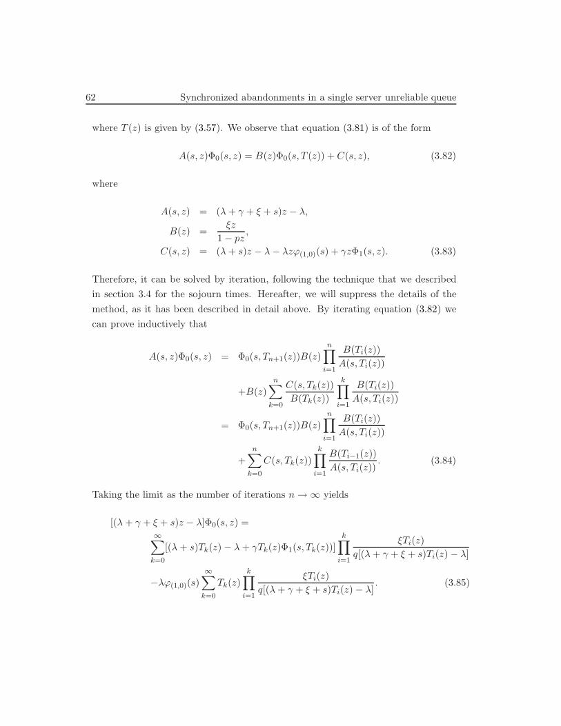
62 Synchronized abandonments in a single server unreliable queue
where T (z) is given by (3.57). We observe that equation (3.81) is of the form
A(s, z)$0(s, z) = B(z)$0(s, T (z)) + C(s, z), (3.82)
where
A(s, z) = (" + ) + ' + s)z ! ",
B(z) ='z
1 ! pz,
C(s, z) = (" + s)z ! "! "z&(1,0)(s) + )z$1(s, z). (3.83)
Therefore, it can be solved by iteration, following the technique that we described
in section 3.4 for the sojourn times. Hereafter, we will suppress the details of the
method, as it has been described in detail above. By iterating equation (3.82) we
can prove inductively that
A(s, z)$0(s, z) = $0(s, Tn+1(z))B(z)n*
i=1
B(Ti(z))
A(s, Ti(z))
+B(z)n$
k=0
C(s, Tk(z))
B(Tk(z))
k*
i=1
B(Ti(z))
A(s, Ti(z))
= $0(s, Tn+1(z))B(z)n*
i=1
B(Ti(z))
A(s, Ti(z))
+n$
k=0
C(s, Tk(z))k*
i=1
B(Ti$1(z))
A(s, Ti(z)). (3.84)
Taking the limit as the number of iterations n " # yields
[(" + ) + ' + s)z ! "]$0(s, z) =#$
k=0
[(" + s)Tk(z) ! " + )Tk(z)$1(s, Tk(z))]k*
i=1
'Ti(z)
q[(" + ) + ' + s)Ti(z) ! "]
!"&(1,0)(s)#$
k=0
Tk(z)k*
i=1
'Ti(z)
q[(" + ) + ' + s)Ti(z) ! "]. (3.85)
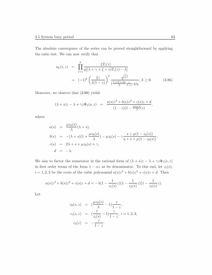
3.5 System busy period 63
The absolute convergence of the series can be proved straightforward by applying
the ratio test. We can now verify that
ak(s, z) =k*
i=1
'Ti(z)
q[(" + ) + ' + s)Ti(z) ! "]
= (!1)k.
'z
"(1 ! z)
/k q(k2)
( (&+'+s)q"
z1$z ; q)k
, k $ 0. (3.86)
Moreover, we observe that (3.80) yields
(" + s)z ! " + )z$1(s, z) =a(s)z3 + b(s)z2 + c(s)z + d
(1 ! z)(1 ! µz0(s)" z)
,
where
a(s) =µz0(s)
"(" + s),
b(s) = !(" + s)(1 +µz0(s)
") ! µz0(s) ! )
s + µ(1 ! z0(s))
( + s + µ(1 ! z0(s)),
c(s) = 2" + s + µz0(s) + ),
d = !".
We aim to factor the numerator in the rational form of (" + s)z ! " + )z$1(s, z)
in first order terms of the form 1 ! *z as its denominator. To this end, let zi(s),
i = 1, 2, 3 be the roots of the cubic polynomial a(s)z3 + b(s)z2 + c(s)z + d. Then
a(s)z3 + b(s)z2 + c(s)z + d = !"(1 !1
z1(s)z)(1 !
1
z2(s)z)(1 !
1
z3(s)z).
Let
c0(s, z) = (µz0(s)
"! 1)
z
1 ! z,
ci(s, z) = (1
zi(s)! 1)
z
1 ! z, i = 1, 2, 3,
c4(z) = !z
1 ! z.

64 Synchronized abandonments in a single server unreliable queue
We then have that
(" + s)Tk(z) ! " + )Tk(z)$1(s, Tk(z)) =
!"(1 ! c1(s, z)qk)(1 ! c2(s, z)qk)(1 ! c3(s, z)qk)
(1 ! c0(s, z)qk)(1 ! c4(z)qk),
a rational function of qk. Then, we can easily see that
(" + s)Tk(z) ! " + )Tk(z)$1(s, Tk(z))
can be expressed using q–factorials in the form
(" + s)Tk(z) ! " + )Tk(z)$1(s, Tk(z)) =
!"(1 ! c1(s, z))(1 ! c2(s, z))(1 ! c3(s, z))
(1 ! c0(s, z))(1 ! c4(z))bk(s, z), (3.87)
where bk(s, z) are given by
bk(s, z) =(c0(s, z), c1(s, z)q, c2(s, z)q, c3(s, z)q, c4(z); q)k(c0(s, z)q, c1(s, z), c2(s, z), c3(s, z), c4(z)q; q)k
, k $ 0. (3.88)
Then equation (3.85) can be written as
[(" + ) + ' + s)z ! "]$0(s, z) =
!"(1 ! c1(s, z))(1 ! c2(s, z))(1 ! c3(s, z))
(1 ! c0(s, z))(1 ! c4(z))
#$
k=0
ak(s, z)bk(s, z)
!"&(1,0)(s)#$
k=0
ak(s, z)Tk(z). (3.89)
We set z = ""+&+'+s in (3.89) and define ci(s) = ci(s,
""+&+'+s), i = 0, 1, 2, 3 and
c4(s) = c4("
"+&+'+s). Then, after reducing the sums in the canonical form of the
q–series, (3.89) yields
&(1,0)(s) = !() + ' + s + ")(1 ! c1(s))(1 ! c2(s))(1 ! c3(s))
"(1 ! c0(s))(1 ! c4(s)) 1!1(c4(s); c4(s)q; q,'q
&+'+s)
) 5!5
"
c0(s), c1(s)q, c2(s)q, c3(s)q, c4(s)
c0(s)q, c1(s), c2(s), c3(s), c4(s)q; q,
'
) + ' + s
#
. (3.90)
3.5 System busy period 65
We can now use (3.78) and (3.90) to obtain &L(s). Although the symbolic inversion
of &L(s) is not possible, one can perform numerical inversion to obtain the distri-
bution of the busy period L or other associated measures (see e.g. Abate et al.
(2000)).

66 Synchronized abandonments in a single server unreliable queue
Chapter 4
Synchronized reneging in
single server vacation queues
Part I
In chapters 4 and 5 we present a detailed analysis of two fundamental queueing
models with vacations and impatient customers, where the source of impatience is
the absence of the server. Instead of the standard assumption that customers per-
form independent abandonments, we consider situations where customers abandon
the system simultaneously. This is, for example, the case in remote systems where
customers may decide to abandon the system, when a transport facility becomes
available. In chapter 4 we study the Markovian case, while in chapter 5 we study
the non-Markovian counterparts.
4.1 Introduction
Queueing systems with reneging (i.e., impatient customers) have been studied exten-
sively. The main assumption in the literature is that customers perform independent
abandonments, that is, each one of them sets an impatience clock and abandons the
system as soon as the clock expires. For Markovian models, this type of abandon-
68 Synchronized reneging in single server vacation queues – Part I
ments introduces state-inhomogeneous transition rate matrices, a fact that compli-
cates the computation of the performance measures. For non-Markovian models,
the basic idea is to use the methodology from the study of the M/G/# queue. In
both cases, however, it seems fair to say that most of the models are analytically
intractable.
The study of queueing systems with impatient customers goes back at least to
the pioneering papers of Palm (1953, 1957) who studied the M/M/c queue, where
the customers have independent exponentially distributed impatience times. Subse-
quently, Daley (1965), Takacs (1974) and Baccelli et al. (1984) considered various
queueing models with general service and/or inter-arrival times and more involved
abandonment schemes.
More recently, Boxma and de Waal (1994) studied the M/M/c queue with gen-
erally distributed impatience times, while Altman and Borovkov (1997) investigated
the stability issue in a retrial queue with impatient customers. In all the afore-
mentioned works, customers become impatient due to the long waiting time already
experienced, although the server provides continuously service. The study of reneg-
ing within the class of queueing systems with vacations is a new endeavor. Although,
there exists a significant number of papers and books on vacation queueing systems
(see, e.g., Takagi (1991) and Tian and Zhang (2006)), the reneging feature has not
yet received much attention. Only recently, Altman and Yechiali (2006) and Yechiali
(2007) considered systems with vacations, where the cause of the impatience is the
absence of the server. The authors assume that the customers perform independent
abandonments, whenever the server is unavailable.
In chapters 4 and 5, we study two models with vacations, where the customers
are impatient but they perform synchronized abandonments. These models are mo-
tivated by remote systems where customers have to wait for a certain transport
facility to abandon the system. Then, whenever the facility visits the system, the
present customers decide whether to leave the system or not. Therefore, we have
synchronized departures for some of the customers. In chapter 4 we deal with the

4.2 Model description 69
Markovian cases, while in chapter 5 we treat the general times cases.
The first model is the single-server queue with multiple vacations, where cus-
tomers decide whether to abandon the system or not when the vacation periods
finish. In the second model, we suppose that the abandonments opportunities occur
according to a Poisson process during vacation periods. At the abandonment oppor-
tunities, every present customer remains in the system with probability q or aban-
dons the system with probability p = 1!q, independently of the others. The analysis
of this model extends the analysis of Altman and Yechiali (2006), in the framework of
synchronized abandonments. The new feature of these models with synchronization
is the presence of binomial type jumps at the abandonment epochs. Similar models
with binomial type transitions have been recently studied by Economou (2004), Ar-
talejo et al. (2007), Economou and Fakinos (2008).
Chapter 4 is organized as follows. In Section 4.2, we describe the dynamics of
the models. In Section 4.3 we carry out a mean value analysis of the two models.
In Section 4.4 we present, separately, the stationary analysis of the two models.
We also obtain more explicit results under various limiting regimes concerning the
parameters of the models.
4.2 Model description
We consider a queueing system where customers arrive one by one according to a
Poisson process at rate ". Service is provided by a single server who can be in one
of two modes: on (active) or o" (non-active - on vacation). Customers are served
singly when the server is on, while no service is provided when the server is o".
The service times, B, are exponentially distributed with rate µ, where the random
variable B represents the service time. There is infinite waiting room. Whenever the
system becomes empty, the server begins a vacation, V , where the random variable
V represents the vacation time. We assume multiple vacations, i.e., if the system
is still empty at the end of a vacation, the server takes another one. If, on the
contrary, there is at least one waiting customer at the end of a vacation, the server
70 Synchronized reneging in single server vacation queues – Part I
starts again to provide service. The vacation times are exponentially distributed
with rate ). Regarding the abandonments we consider two models:
• Unique Abandonment Epoch (UAE) : Every time the server finishes a vacation,
every present customer decides whether to stay in the system with probability
q or to abandon it with probability p = 1 ! q, independently of the others.
• Multiple Abandonment Epochs (MAE) : During server vacations, abandon-
ment opportunities occur according to a Poisson process with rate +. At these
epochs, every present customer remains in the system with probability q or
abandons the system with probability p = 1 ! q, independently of the others.
Hence, in either model, the number of customers is reduced according to a bino-
mial distribution at every abandonment epoch. However, the analysis of the UAE
model turns out to be much easier than the one of the MAE model. For this reason,
in what follows, we describe briefly the results for the UAE model and we provide
more details for the analysis of the MAE model.
We are interested in the equilibrium behavior of the model, so we need to establish
first the stability condition. For the pure vacation model (p = 0) the stability
condition is (see, e.g., Takagi (1991))
, ="
µ< 1. (4.1)
Hence, the above condition is su!cient for the stability of the UAE and MAE models.
It is also necessary, since the system behaves as a standard M/M/1 queue while the
server is active. Clearly, the only exception is the degenerate case p = 1 for the UAE
model. Then condition (4.1) is not required for stability. Throughout the chapter
we assume the validity of condition (4.1).
4.3 Mean value analysis 71
4.3 Mean value analysis
4.3.1 Mean value analysis of the UAE model
We suppose that the system is in equilibrium and we define the random variable
L to be the number of customers in the system and S to be the sojourn time of a
customer. Let also Li be the conditional number of customers in the system, given
that the server is in state i, i = 0, 1. Further we denote by pi the probability (or
fraction of time) that the server is in state i, i = 0, 1.
Let us consider a tagged arriving customer. Then, by PASTA property, the
probability that this customer finds the server in state i is pi. If he finds the server
providing service, then his mean sojourn time is E(L1)1µ + 1
µ . If he finds the server on
vacation, then he first has to wait for the vacation time to expire; the mean residual
vacation time is 1& . Then, with probability p, he will abandon and, with probability
q, he will remain for service, in which case the mean number of customers that he
will find in front of him is qE(L0). Indeed, by PASTA, he sees at his arrival epoch on
average E(L0) customers in the system and each of them will remain for service with
probability q. So, in this case, his mean sojourn time is 1& + p · 0+ q · (qE(L0)
1µ + 1
µ).
Hence,
E(S) = p1
.
E(L1)1
µ+
1
µ
/
+ p0
.
1
)+ q2E(L0)
1
µ+ q
1
µ
/
. (4.2)
Further, Little’s law states that
E(L) = "E(S), (4.3)
where the unconditional E(L) is related to the conditional ones as
E(L) = p0E(L0) + p1E(L1). (4.4)
Conservation of work gives the relation
p1 = ("p0q + "p1)1
µ, (4.5)
and clearly,
p0 + p1 = 1. (4.6)
72 Synchronized reneging in single server vacation queues – Part I
Finally, by gluing the periods during which the server is on vacation, we observe that
the vacation completion epochs constitute a Poisson process. Hence, by PASTA, we
have that E(L0) coincides with the mean number of customers in the system just
before a vacation time finishes, which is equal to the mean number of Poisson (")
arrivals in a vacation time. Thus,
E(L0) = "1
). (4.7)
Now we have su!ciently many equations for the unknown mean values. Solution of
(4.2)-(4.7) yields the following result.
Theorem 4.1. The mean sojourn time is given by
E(S) =1
1 ! ,p
.
1
)+ (q2 ! 1)
,
)
/
+q
1 ! ,p·
1
µ(1 ! ,), (4.8)
and the fraction of time the server is inactive and active, respectively,
p0 =1 ! ,
1 ! ,p, p1 =
,q
1 ! ,p. (4.9)
4.3.2 Mean value analysis of the MAE model
Let us, again, consider a tagged arriving customer. Then, by PASTA, the probability
that this customer finds the server in state i is pi. If he finds the server providing
service, then his mean sojourn time is E(L1)1µ + 1
µ . If he finds the server on vacation,
then he first has to wait for the vacation time to expire before servicing starts and,
while waiting, he may decide to abandon at one of the abandonment opportunities.
Let E(V &) be his mean time in the system till the end of the vacation; note that
E(V &) will be less than the mean residual vacation time 1& . If the tagged customer
decides to stay till the end of the vacation, then his sojourn time after return of
the server depends on the number of customers (still) in front of him. Define %
as the probability that the tagged customer stays in the system till the end of the
vacation period and define %& as the probability that the tagged customer and a
customer, who was already present at his arrival, both stay in the system. Then
4.3 Mean value analysis 73
%&E(L0)1µ + % 1
µ is his mean sojourn time, from the moment the server returns from
vacation. Hence,
E(S) = p1
.
E(L1)1
µ+
1
µ
/
+ p0
.
E(V &) + %&E(L0)1
µ+ %
1
µ
/
, (4.10)
and Little’s law yields
E(L) = "E(S), (4.11)
where the unconditional E(L) is related to the conditional ones as
E(L) = p0E(L0) + p1E(L1). (4.12)
Also, if we would act as if the customers arriving during a vacation are waiting in
a “vacation area” and transferred to the queue as soon as the server returns, then
application of Little’s law to the vacation area yields
E(L0) = "E(V &). (4.13)
Analogous to (4.5), conservation of work gives the relation
p1 = ("p0% + "p1)1
µ, (4.14)
and clearly,
p0 + p1 = 1. (4.15)
Now we need additional relations for the quantities %, %& and E(V &). By condi-
tioning on the next event after the arrival of the tagged customer, whether it is the
end of the vacation (with probability &)+& ) or an opportunity of abandonment (with
probability ))+& ), we have that
% =)
+ + )· 1 +
+
+ + )q%.
Hence
% =)
+p + ). (4.16)
Along the same lines,
%& =)
+ + )· 1 +
+
+ + )q2%&,
74 Synchronized reneging in single server vacation queues – Part I
so
%& =)
+(1 ! q2) + ). (4.17)
Finally, again conditioning on the next event after the arrival of the tagged customer,
we obtain
E(V &) =1
+ + )+
)
+ + )· 0 +
+
+ + )qE(V &) +
+
+ + )p · 0,
yielding
E(V &) =1
+p + ). (4.18)
This completes the formulation of the mean value relations. By solving (4.10)-(4.15),
taking into account (4.16)-(4.18) we get the following result.
Theorem 4.2. The mean sojourn time is given by
E(S) =1
1 ! , + ,%
.
1
+p + )+ (q2 ! 1)
+%
+(1 ! q2) + )·,
)
/
+%
1 ! , + ,%·
1
µ(1 ! ,)(4.19)
and the fraction of time the server is inactive and active, respectively,
p0 =1 ! ,
1 ! , + ,%, p1 =
,%
1 ! , + ,%. (4.20)
4.4 Equilibrium distribution
We consider the two models described in Section 4.2. Then, each system can be
described by a continuous-time Markov chain {(L(t), I(t)), t $ 0}, with state space
{(0, 0)} + {(n, i) : i = 0, 1, n = 1, 2, . . .}, where L(t) is the number of customers
in the system at time t and I(t) expresses the mode of the server at time t (more
explicitly, it is equal to 1 if the server is on at that time t and 0 otherwise). Below,
we focus on the determination of the equilibrium distribution of the Markov chain
{(L(t), I(t)), t $ 0}. The two models are treated separately.
To this end, let (%(n, i) : i = 0, 1 and n $ i), denote the equilibrium distribution.
We define the (partial) probability generating functions (PGFs) #0(z) and #1(z) of
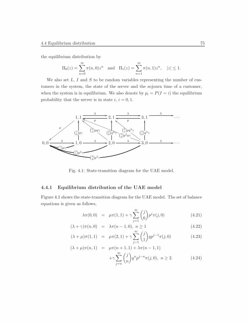
4.4 Equilibrium distribution 75
the equilibrium distribution by
#0(z) =#$
n=0
%(n, 0)zn and #1(z) =#$
n=1
%(n, 1)zn, |z| & 1.
We also set L, I and S to be random variables representing the number of cus-
tomers in the system, the state of the server and the sojourn time of a customer,
when the system is in equilibrium. We also denote by pi = P (I = i) the equilibrium
probability that the server is in state i, i = 0, 1.
1, 1
µ
44!!!!!!!!!!!
!!!!!
" ##2, 1
" ##
µ00 3, 1
" ##
µ00 · · ·
0, 0 " ## 1, 0
(10)q&
--
(11)p&
""" ## 2, 0
(20)q
2&
--
(21)pq&
$$$$$$$
55$$$$$$$
(22)p
2&
33" ## 3, 0
(30)q
3&
--
(31)pq2&
$$$$$$$
55$$$$$$$
(32)p
2q&%%%%%%
!!%%%%%%%%%%%%%%%%%%%%
(33)p3&
66" ## · · ·
Fig. 4.1: State-transition diagram for the UAE model.
4.4.1 Equilibrium distribution of the UAE model
Figure 4.1 shows the state-transition diagram for the UAE model. The set of balance
equations is given as follows,
"%(0, 0) = µ%(1, 1) + )#$
j=1
.
j
0
/
pj%(j, 0) (4.21)
(" + ))%(n, 0) = "%(n ! 1, 0), n $ 1 (4.22)
(" + µ)%(1, 1) = µ%(2, 1) + )#$
j=1
.
j
1
/
qpj$1%(j, 0) (4.23)
(" + µ)%(n, 1) = µ%(n + 1, 1) + "%(n ! 1, 1)
+)#$
j=n
.
j
n
/
qnpj$n%(j, 0), n $ 2. (4.24)
76 Synchronized reneging in single server vacation queues – Part I
Provided (4.1), this set of equations, together with the normalization equation
%(0, 0) +#$
n=1
(%(n, 0) + %(n, 1)) = 1,
has a unique solution. This solution is presented in the next theorem.
Theorem 4.3. Provided (4.1), the equilibrium state distribution %(n, i) is given by
%(0, 0) =)
) + "·
1 ! ,
1 ! ,p(4.25)
%(n, 0) = %(0, 0)
.
"
" + )
/n
, n $ 0 (4.26)
%(n, 1) =
'
(
)
%(0, 0) ("+&)q&+("$µ)q
2
,n !2
"q&+"q
3n3
, if ) (= (µ ! ")q
%(0, 0)(,p + q)n,n, if ) = (µ ! ")q, n $ 1.(4.27)
Proof. By iterating (4.22) we obtain (4.26) yielding
#0(z) =" + )
" + ) ! "z%(0, 0). (4.28)
By multiplying (4.23) by z and (4.24) by zn and adding for all n = 1, 2, . . . we obtain
(" + µ)#1(z) = "z#1(z) +µ
z(#1(z) ! z%(1, 1)) + )#0(p + qz) ! )#0(p). (4.29)
Solving (4.29) for #1(z) and plugging (4.28), while using (4.21), yields
#1(z) =q,z() + ")
() + "q(1 ! z))(1 ! ,z)%(0, 0). (4.30)
Expanding (4.30), for the case ) (= (µ ! ")q, in partial fractions and using the
geometric series leads to the upper branch of (4.27). For the case ) = (µ ! ")q,
expanding (1 ! ,z)$2 in power series and equating the coe!cients of zn yields the
other branch of (4.27). Finally, (4.25) follows from the normalization equation. !
4.4 Equilibrium distribution 77
Remark 4.1. From equations (4.28) and (4.30) we obtain the equilibrium mean
number of customers in the system given as
E(L) =#$
n=1
n(%(n, 0) + %(n, 1))
= #"0(1) + #"
1(1)
= %(0, 0)" + )
)·"
)+ %(0, 0)
(" + ))q,
)(1 ! ,)·)(1 ! ,) + ,) + "q(1 ! ,)
)(1 ! ,)
= p0"
)+ p1
) + "q(1 ! ,)
)(1 ! ,).
This result can be alternatively derived using the mean value approach, as showed
in Section 4.3.
Remark 4.2. Let X(*) denote an exponential random variable with rate * and
Y (j,*) denote an Erlang random variable consisting of j phases with rate *. Let
us consider a tagged arriving customer. Then, by the PASTA property, he finds the
system in state (n, i) with probability %(n, i). If he finds the system in state (n, 1),
then his sojourn time is Y (n + 1, µ). If he finds the system in state (n, 0), then with
probability p his sojourn time will be X()), since the tagged customer abandons the
system, and with probability,n
j
-
pn$jqj+1 his sojourn time will be X())+Y (j+1, µ),
for j = 0, 1, . . . , n, where the random variables X()) and Y (j+1, µ) are independent.
Hence, by using the geometric form of the equilibrium distribution (4.25)-(4.27), we
have that the LST of the sojourn time S(s) = E(e$sS) can be represented as
S(s) = p0p)
) + s+ p0q
)
) + s·
)µ
)µ + () + q")s+ p1
µ ! "
µ ! " + s·
)µ
)µ + () + q")s.
This shows that the sojourn time S is a mixture of X()), X()) + X( &µ&+q" ), X(µ !
") + X( &µ&+q" ) with mixing probabilities p0p, p0q and p1, respectively.
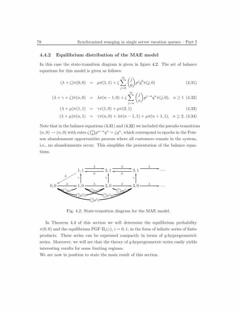
78 Synchronized reneging in single server vacation queues – Part I
4.4.2 Equilibrium distribution of the MAE model
In this case the state-transition diagram is given in figure 4.2. The set of balance
equations for this model is given as follows:
(" + +)%(0, 0) = µ%(1, 1) + +#$
j=0
.
j
0
/
pjq0%(j, 0) (4.31)
(" + ) + +)%(n, 0) = "%(n ! 1, 0) + +#$
j=n
.
j
n
/
pj$nqn%(j, 0), n $ 1 (4.32)
(" + µ)%(1, 1) = )%(1, 0) + µ%(2, 1) (4.33)
(" + µ)%(n, 1) = )%(n, 0) + "%(n ! 1, 1) + µ%(n + 1, 1), n $ 2. (4.34)
Note that in the balance equations (4.31) and (4.32) we included the pseudo-transitions
(n, 0) " (n, 0) with rates +,n0
-
pn$nqn = +qn, which correspond to epochs in the Pois-
son abandonment opportunities process where all customers remain in the system,
i.e., no abandonments occur. This simplifies the presentation of the balance equa-
tions.
1, 1µ
%%&&&&&&&&&&&&
" ##2, 1
" ##
µ00 3, 1
" ##
µ00 · · ·
0, 0 " ## 1, 0
&
--
(11)p)
33" ## 2, 0
&
--
(21)pq)
33
(22)p
2)
66" ## 3, 0
&
--
(31)pq2)
33
(32)p
2q)
66
(33)p
3)
77" ## · · ·
Fig. 4.2: State-transition diagram for the MAE model.
In Theorem 4.4 of this section we will determine the equilibrium probability
%(0, 0) and the equilibrium PGF #i(z), i = 0, 1, in the form of infinite series of finite
products. These series can be expressed compactly in terms of q-hypergeometric
series. Moreover, we will see that the theory of q-hypergeometric series easily yields
interesting results for some limiting regimes.
We are now in position to state the main result of this section.
4.4 Equilibrium distribution 79
Theorem 4.4. Provided (4.1), the equilibrium state probability of an empty system
%(0, 0) is given by
%(0, 0) =A
+
#$
j=0
j*
k=0
+
) + + + "qk
=A
) + +
(q; q)#
(! "&+) ,
)&+) ; q)#
2!1
.
!"
) + +,
+
) + +; 0; q, q
/
. (4.35)
The partial PGFs #0(z) and #1(z) are given by
#0(z) =A
+
#$
j=0
j*
k=0
+
) + + + "qk(1 ! z)(4.36)
=A
) + +
(q; q)#
(!"(1$z)&+) , )
&+) ; q)#2!1
.
!"(1 ! z)
) + +,
+
) + +; 0; q, q
/
(4.37)
#1(z) = !Az
"z + µz ! "z2 ! µ+
)z
"z + µz ! "z2 ! µ#0(z), (4.38)
where
A =)(µ ! ")() + +(1 ! q))
µ) + (µ ! ")+(1 ! q). (4.39)
The convergence of the series is absolute in {z % C : |z| & 1} and uniform in every
compact subset of {z % C : |z| < 1}.
Proof. Multiplying both sides of equations (4.31) and (4.32) by z0 and zn, respec-
tively, and summing them for all n = 0, 1, 2, . . . we obtain
(" + ) + +)#0(z) ! )%(0, 0) = µ%(1, 1) + "z#0(z) + +#$
n=0
#$
j=n
.
j
n
/
pj$nqn%(j, 0)zn
or
(" + ) + + ! "z)#0(z) = )%(0, 0) + µ%(1, 1) + +#0(1 ! q + qz), (4.40)
which leads to
#0(z) =)%(0, 0) + µ%(1, 1)
) + + + "(1 ! z)+
+
) + + + "(1 ! z)#0(1 ! q + qz). (4.41)
80 Synchronized reneging in single server vacation queues – Part I
Furthermore, by multiplying both sides of equations (4.33) and (4.34) by z and
zn, respectively, and summing them for all n = 1, 2, 3, . . . we obtain after some
rearrangements that
#1(z) = !()%(0, 0) + µ%(1, 1))z
"z + µz ! "z2 ! µ+
)z
"z + µz ! "z2 ! µ#0(z). (4.42)
By iterating equation (4.41) and setting
A = )%(0, 0) + µ%(1, 1) (4.43)
we obtain
#0(z) =A
+
n$
j=0
j*
k=0
+
) + + + "qk(1 ! z)
+#0(1 ! qn+1 + qn+1z)n*
k=0
+
) + + + "qk(1 ! z), n $ 0. (4.44)
By letting n " # we get
#0(z) =A
+
#$
j=0
j*
k=0
+
) + + + "qk(1 ! z), (4.45)
which is expressed as a q-hypergeometric series in the form (4.37). This shows also
that the infinite series does converge. We set z = 0 in (4.45), yielding
%(0, 0) =A
+
#$
j=0
j*
k=0
+
) + + + "qk, (4.46)
which can be put in the form (4.35). We set z = 1 in (4.45), which leads to
#0(1) =A
+
#$
j=0
j*
k=0
+
) + +=
A
). (4.47)
Note also that by (4.42), (4.43) and (4.47) we obtain
#1(1) =)
µ ! "#"
0(1). (4.48)
4.4 Equilibrium distribution 81
To obtain #"0(1) multiply (4.41) by ) + + + "(1 ! z), di"erentiate and take z " 1.
We then have
#"0(1) =
"A
)() + +(1 ! q)). (4.49)
Equations (4.48) and (4.49) yield
#1(1) ="A
(µ ! ")() + +(1 ! q)). (4.50)
We have now expressed the various quantities of interest and the PGFs #0(z) and
#1(z) in terms of the parameters of the model and the parameter A. Using (4.47) and
(4.50) and the normalization equation we obtain (4.39) which concludes the proof. !
Remark 4.3. By di"erentiating twice (4.42) and once (4.41) and taking z " 1
we obtain, after some long calculations, the mean number of customers in system.
However, as we have showed in Section 4.3, the mean value approach gives the result
much more easily.
4.4.3 Fluid limit of the UAE model
In this section we study the scaled queue length process in the UAE model as both
the arrival rate " and service rate µ tend to infinity, while keeping the tra!c intensity
, = "µ fixed. That is, we consider the sequence of queue length processes Lm(t) with
arrival rates "m = m", service rates µm = mµ and constant vacation rate )m = ),
and then we are interested in obtaining the equilibrium distribution of the fluid
scaled limit
L(t) = limm%#
Lm(t)
m.
The fluid scaled sample path of Lm(t) is shown in figure 4.3. Clearly, a cycle first
starts with an exponential vacation V , at the start of which there is no fluid and
during which the amount of fluid increases with rate ". At the end of the vacation
an exponential amount X = "V has been accumulated in the queue; a fraction p
of X will then immediately abandon and the remainder qX will be drained at rate
µ! ", which takes an exponential time P = qX/(µ ! "). When the queue is empty
again, the cycle repeats.
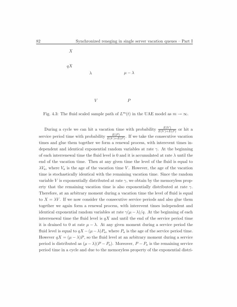
82 Synchronized reneging in single server vacation queues – Part I
V P
" µ ! "
X
qX
Fig. 4.3: The fluid scaled sample path of Lm(t) in the UAE model as m " #.
During a cycle we can hit a vacation time with probability E(V )E(V )+E(P ) or hit a
service period time with probability E(P )E(V )+E(P ) . If we take the consecutive vacation
times and glue them together we form a renewal process, with interevent times in-
dependent and identical exponential random variables at rate ). At the beginning
of each interrenewal time the fluid level is 0 and it is accumulated at rate " until the
end of the vacation time. Then at any given time the level of the fluid is equal to
"Va, where Va is the age of the vacation time V . However, the age of the vacation
time is stochastically identical with the remaining vacation time. Since the random
variable V is exponentially distributed at rate ), we obtain by the memoryless prop-
erty that the remaining vacation time is also exponentially distributed at rate ).
Therefore, at an arbitrary moment during a vacation time the level of fluid is equal
to X = "V . If we now consider the consecutive service periods and also glue them
together we again form a renewal process, with interevent times independent and
identical exponential random variables at rate )(µ!")/q. At the beginning of each
interrenewal time the fluid level is qX and until the end of the service period time
it is drained to 0 at rate µ ! ". At any given moment during a service period the
fluid level is equal to qX ! (µ!")Pa, where Pa is the age of the service period time.
However qX = (µ ! ")P , so the fluid level at an arbitrary moment during a service
period is distributed as (µ! ")(P !Pa). Moreover, P !Pa is the remaining service
period time in a cycle and due to the memoryless property of the exponential distri-
4.4 Equilibrium distribution 83
bution is stochastically identical to P , therefore the amount of fluid at an arbitrary
time of the service period is equal to (µ ! ")P = qX.
Let the random variable L denote the amount of fluid in the queue, when the
system is in equilibrium. From the memoryless property of exponentials, we imme-
diately obtain
Ld=
7
X w.p. E(V )E(V )+E(P ) ,
qX w.p. E(P )E(V )+E(P ) ,
(4.51)
where
E(V ) =1
), E(P ) =
q
µ ! ""E(V ) =
q,
1 ! ,
1
).
In addition to the above intuitive derivation of equation (4.51), we prove the follow-
ing theorem by directly employing (4.25), (4.28) and (4.30).
Theorem 4.5. The LST of L is given by
E(e$sL) =1 ! ,
1 ! , + q,
&"
&" + s
+q,
1 ! , + q,
&q"&q" + s
.
Proof . We can determine the LST of L as the limit of E(e$sLm/m) as m " #,
E(e$sL) = limm%#
E(e$sLm/m)
= limm%#
[#(m)0 (e$s/m) + #(m)
1 (e$s/m)]
= limm%#
0
m" + )
m" + ) ! m"e$s/m
)
) + m"
1 ! ,
1 ! p,
+q,e$s/m() + m")
() + m"q(1 ! e$s/m))(1 ! ,e$s/m)
)
) + m"
1 ! ,
1 ! p,
5
= limm%#
0
)
) + m"(1 ! e$s/m)
1 ! ,
1 ! p,
+q,e$s/m)
() + m"q(1 ! e$s/m))(1 ! ,e$s/m)
1 ! ,
1 ! p,
5
.
Since
limm%#
m(1 ! e$s/m) = s, (4.52)
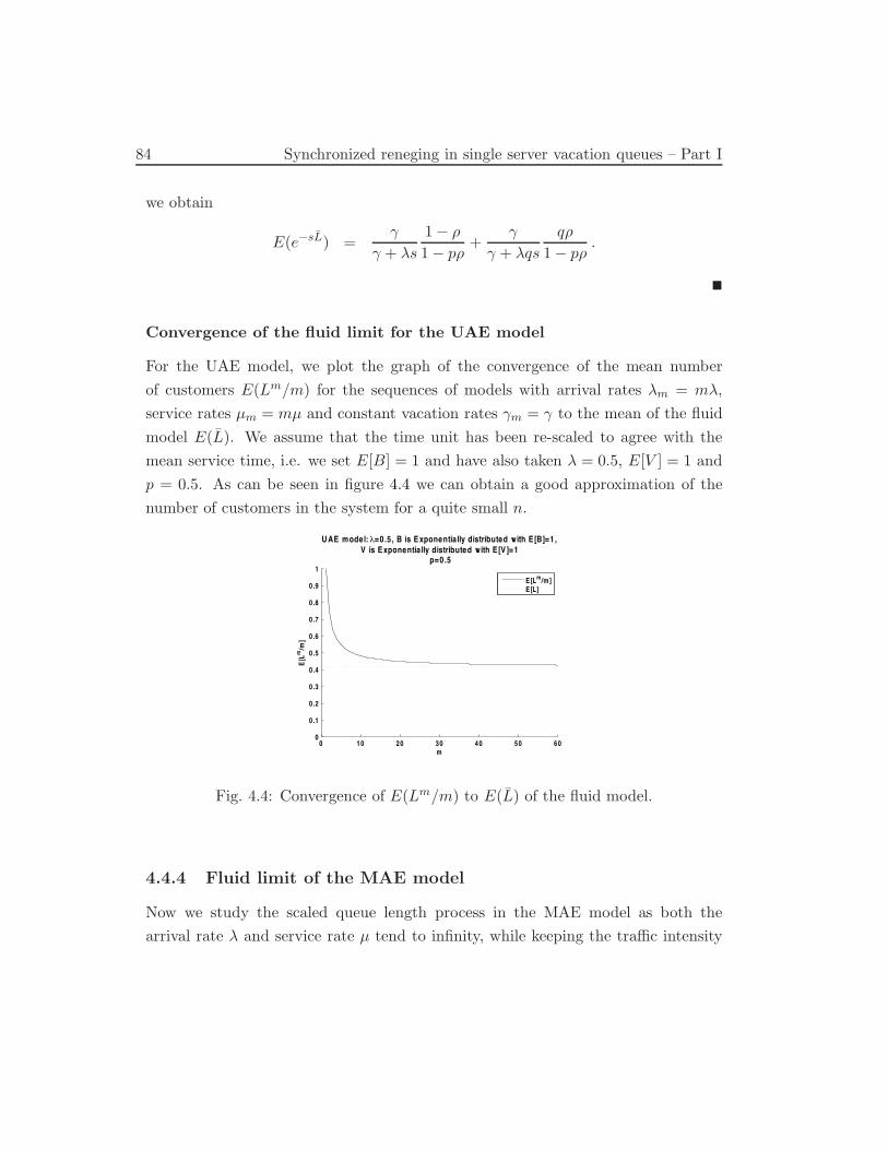
84 Synchronized reneging in single server vacation queues – Part I
we obtain
E(e$sL) =)
) + "s
1 ! ,
1 ! p,+
)
) + "qs
q,
1 ! p,.
!
Convergence of the fluid limit for the UAE model
For the UAE model, we plot the graph of the convergence of the mean number
of customers E(Lm/m) for the sequences of models with arrival rates "m = m",
service rates µm = mµ and constant vacation rates )m = ) to the mean of the fluid
model E(L). We assume that the time unit has been re-scaled to agree with the
mean service time, i.e. we set E[B] = 1 and have also taken " = 0.5, E[V ] = 1 and
p = 0.5. As can be seen in figure 4.4 we can obtain a good approximation of the
number of customers in the system for a quite small n.
0 10 20 30 40 50 600
0.1
0 .2
0 .3
0 .4
0 .5
0 .6
0 .7
0 .8
0 .9
1
m
E[L
m/m
]
U AE model: λ=0.5 , B is E xponentia lly distributed with E [B]=1,V is E xponentia lly distributed with E [V ]=1
p=0.5
E [Lm/m]E [L]
Fig. 4.4: Convergence of E(Lm/m) to E(L) of the fluid model.
4.4.4 Fluid limit of the MAE model
Now we study the scaled queue length process in the MAE model as both the
arrival rate " and service rate µ tend to infinity, while keeping the tra!c intensity
4.4 Equilibrium distribution 85
, = "µ fixed. So we consider the sequence of queue length processes Lm(t) with
arrival rates "m = m", service rates µm = mµ and constant vacation rates )m = )
and abandonment rates +m = +. We are interested in obtaining the equilibrium
distribution of the fluid scaled limit
L(t) = limm%#
Lm(t)
m.
The fluid scaled sample path of Lm(t) is shown in figure 4.5. The cycle starts
with an empty queue and a random number of exponential vacations V1, . . . , VN ,
each with mean 1&+) and during which the amount of fluid increases with rate ".
The amount of fluid that is added during Vn is Xn = "Vn. The number of vacations
is geometrically distributed with success probability &)+& ,
P (N = n) =
.
+
+ + )
/n$1 )
+ + ), n = 1, 2, . . . .
At the end of each vacation Vn, a fraction p of the total amount of fluid in the queue
will instantly abandon. The only exception is the last vacation VN . At the end of
VN no fluid is removed, since this is not an abandonment epoch, but the end of the
vacation period. The total amount of fluid in the queue at the end of VN is denoted
by the random variable Z; so
Z =N$
n=1
qN$nXn.
Subsequently the service period starts, during which the queue is drained at rate
µ ! ". The time required to empty the queue is P = Z/(µ ! "). Finally, when the
queue is empty, the cycle repeats.
As before, let the random variable L denote the amount of fluid in the queue, when
the system is in equilibrium. Further, let Li be the amount of fluid in the queue,
given that the server is in state i, i = 0, 1. During a cycle we can hit a vacation
period V , where V =!N
i=1 Vi, with probability E(V )E(V )+E(P ) or hit a service period
time with probability E(P )E(V )+E(P ) . We observe that V is exponentially distributed
at rate ), since Viiid, Exp() + +) and N is independent of Vi and is geometrically
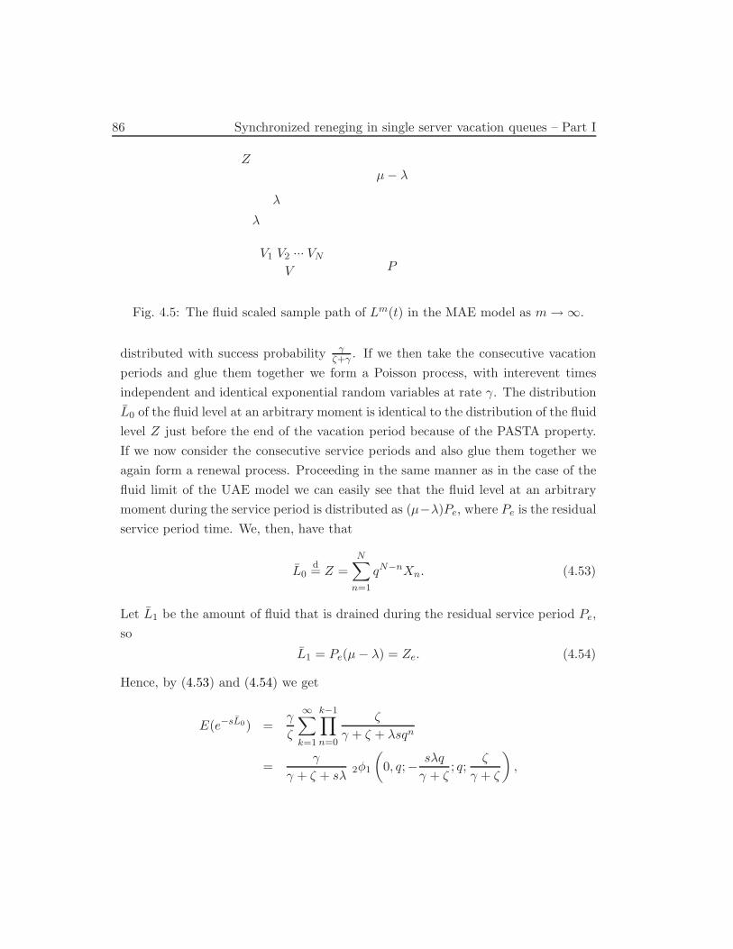
86 Synchronized reneging in single server vacation queues – Part I
V
V1 V2 ... VNP
"
"
µ ! "Z
Fig. 4.5: The fluid scaled sample path of Lm(t) in the MAE model as m " #.
distributed with success probability &)+& . If we then take the consecutive vacation
periods and glue them together we form a Poisson process, with interevent times
independent and identical exponential random variables at rate ). The distribution
L0 of the fluid level at an arbitrary moment is identical to the distribution of the fluid
level Z just before the end of the vacation period because of the PASTA property.
If we now consider the consecutive service periods and also glue them together we
again form a renewal process. Proceeding in the same manner as in the case of the
fluid limit of the UAE model we can easily see that the fluid level at an arbitrary
moment during the service period is distributed as (µ!")Pe, where Pe is the residual
service period time. We, then, have that
L0d= Z =
N$
n=1
qN$nXn. (4.53)
Let L1 be the amount of fluid that is drained during the residual service period Pe,
so
L1 = Pe(µ ! ") = Ze. (4.54)
Hence, by (4.53) and (4.54) we get
E(e$sL0) =)
+
#$
k=1
k$1*
n=0
+
) + + + "sqn
=)
) + + + s"2!1
.
0, q;!s"q
) + +; q;
+
) + +
/
,
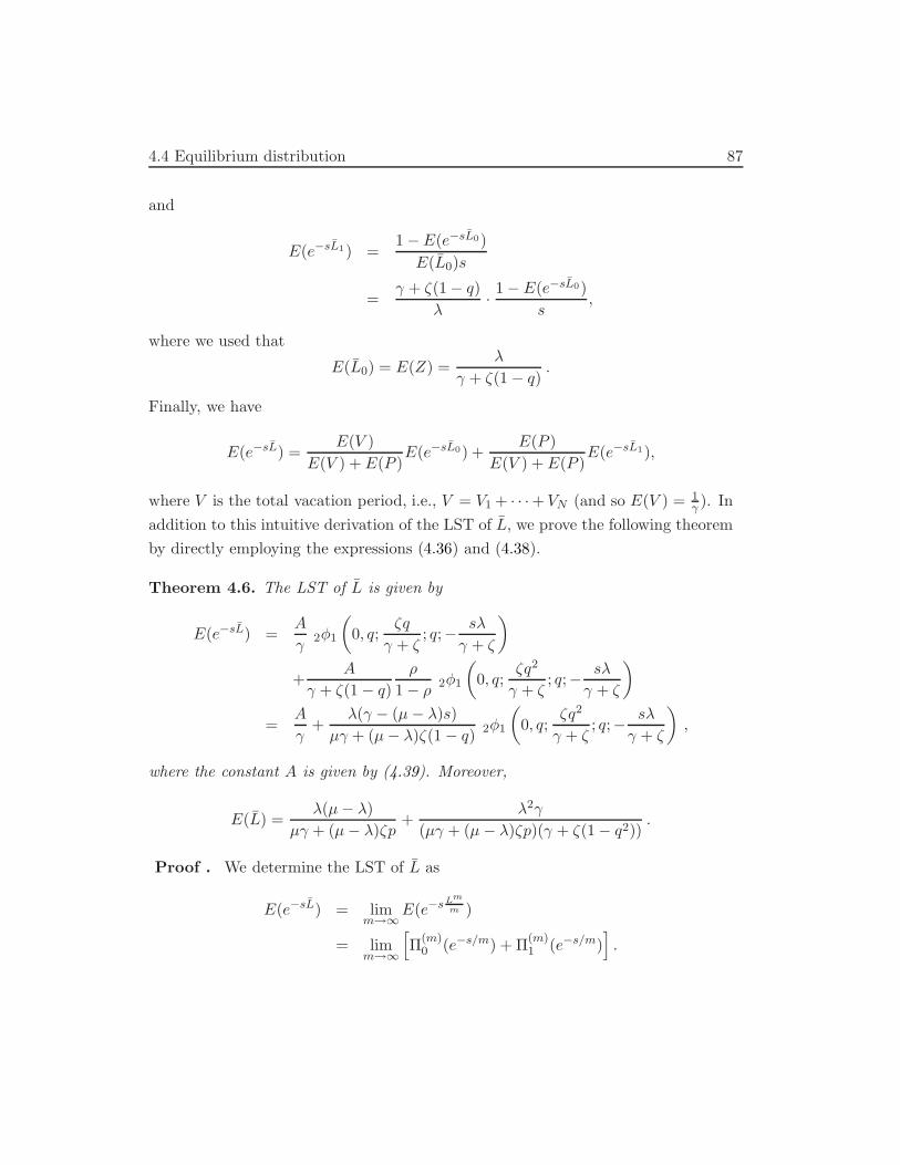
4.4 Equilibrium distribution 87
and
E(e$sL1) =1 ! E(e$sL0)
E(L0)s
=) + +(1 ! q)
"·1 ! E(e$sL0)
s,
where we used that
E(L0) = E(Z) ="
) + +(1 ! q).
Finally, we have
E(e$sL) =E(V )
E(V ) + E(P )E(e$sL0) +
E(P )
E(V ) + E(P )E(e$sL1),
where V is the total vacation period, i.e., V = V1 + · · ·+ VN (and so E(V ) = 1& ). In
addition to this intuitive derivation of the LST of L, we prove the following theorem
by directly employing the expressions (4.36) and (4.38).
Theorem 4.6. The LST of L is given by
E(e$sL) =A
)2!1
.
0, q;+q
) + +; q;!
s"
) + +
/
+A
) + +(1 ! q)
,
1 ! , 2!1
.
0, q;+q2
) + +; q;!
s"
) + +
/
=A
)+
"() ! (µ ! ")s)
µ) + (µ ! ")+(1 ! q) 2!1
.
0, q;+q2
) + +; q;!
s"
) + +
/
,
where the constant A is given by (4.39). Moreover,
E(L) ="(µ ! ")
µ) + (µ ! ")+p+
"2)
(µ) + (µ ! ")+p)() + +(1 ! q2)).
Proof . We determine the LST of L as
E(e$sL) = limm%#
E(e$s Lm
m )
= limm%#
%
#(m)0 (e$s/m) + #(m)
1 (e$s/m)&
.
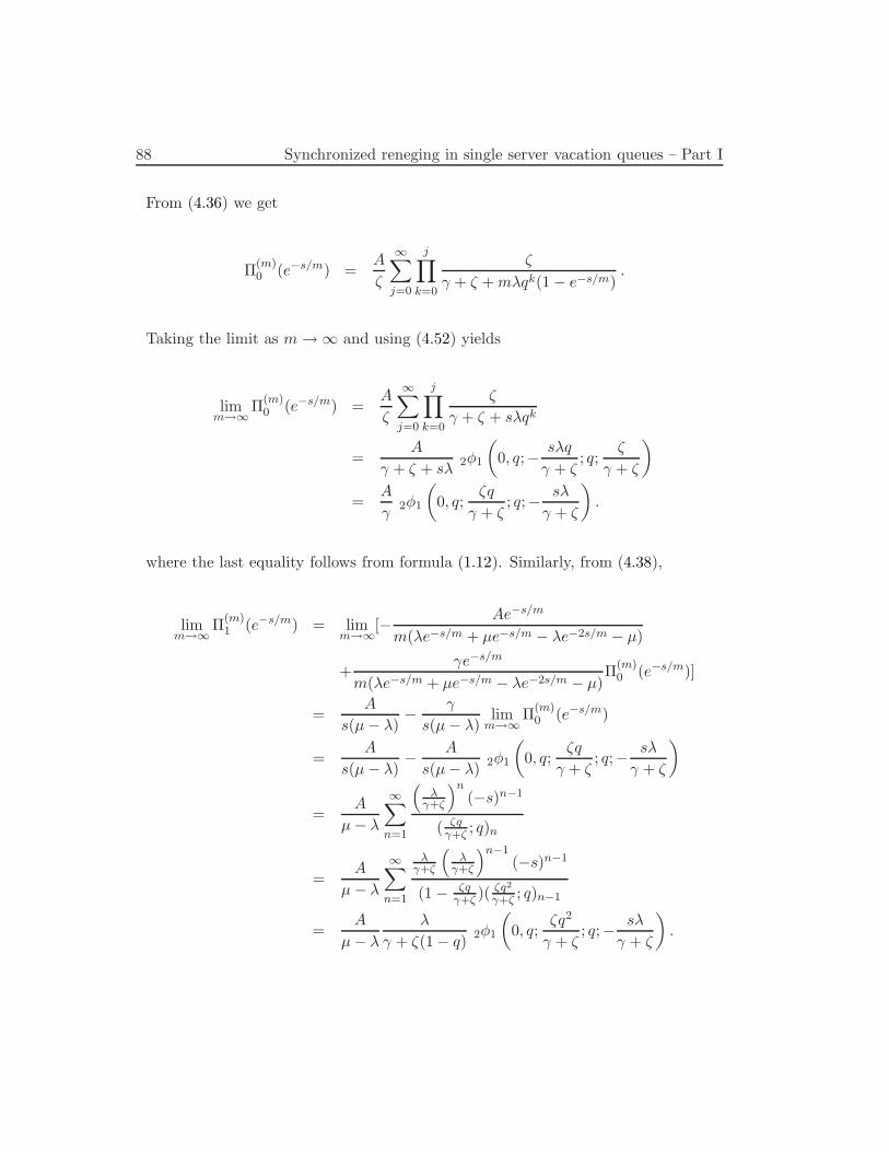
88 Synchronized reneging in single server vacation queues – Part I
From (4.36) we get
#(m)0 (e$s/m) =
A
+
#$
j=0
j*
k=0
+
) + + + m"qk(1 ! e$s/m).
Taking the limit as m " # and using (4.52) yields
limm%#
#(m)0 (e$s/m) =
A
+
#$
j=0
j*
k=0
+
) + + + s"qk
=A
) + + + s" 2!1
.
0, q;!s"q
) + +; q;
+
) + +
/
=A
)2!1
.
0, q;+q
) + +; q;!
s"
) + +
/
.
where the last equality follows from formula (1.12). Similarly, from (4.38),
limm%#
#(m)1 (e$s/m) = lim
m%#[!
Ae$s/m
m("e$s/m + µe$s/m ! "e$2s/m ! µ)
+)e$s/m
m("e$s/m + µe$s/m ! "e$2s/m ! µ)#(m)
0 (e$s/m)]
=A
s(µ ! ")!
)
s(µ ! ")lim
m%##(m)
0 (e$s/m)
=A
s(µ ! ")!
A
s(µ ! ")2!1
.
0, q;+q
) + +; q;!
s"
) + +
/
=A
µ ! "
#$
n=1
2
"&+)
3n(!s)n$1
( )q&+) ; q)n
=A
µ ! "
#$
n=1
"&+)
2
"&+)
3n$1(!s)n$1
(1 ! )q&+) )(
)q2
&+) ; q)n$1
=A
µ ! "
"
) + +(1 ! q)2!1
.
0, q;+q2
) + +; q;!
s"
) + +
/
.
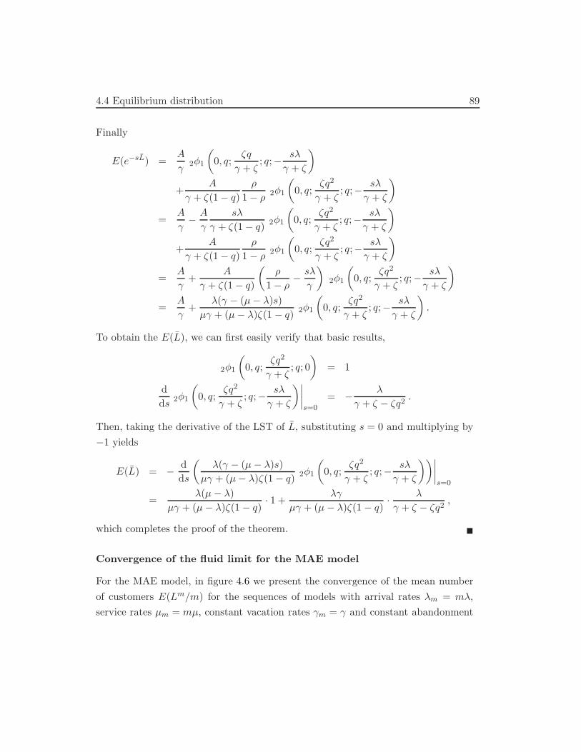
4.4 Equilibrium distribution 89
Finally
E(e$sL) =A
) 2!1
.
0, q;+q
) + +; q;!
s"
) + +
/
+A
) + +(1 ! q)
,
1 ! , 2!1
.
0, q;+q2
) + +; q;!
s"
) + +
/
=A
)!
A
)
s"
) + +(1 ! q) 2!1
.
0, q;+q2
) + +; q;!
s"
) + +
/
+A
) + +(1 ! q)
,
1 ! , 2!1
.
0, q;+q2
) + +; q;!
s"
) + +
/
=A
)+
A
) + +(1 ! q)
.
,
1 ! ,!
s"
)
/
2!1
.
0, q;+q2
) + +; q;!
s"
) + +
/
=A
)+
"() ! (µ ! ")s)
µ) + (µ ! ")+(1 ! q)2!1
.
0, q;+q2
) + +; q;!
s"
) + +
/
.
To obtain the E(L), we can first easily verify that basic results,
2!1
.
0, q;+q2
) + +; q; 0
/
= 1
d
ds 2!1
.
0, q;+q2
) + +; q;!
s"
) + +
/A
A
A
A
s=0
= !"
) + + ! +q2.
Then, taking the derivative of the LST of L, substituting s = 0 and multiplying by
!1 yields
E(L) = !d
ds
.
"() ! (µ ! ")s)
µ) + (µ ! ")+(1 ! q) 2!1
.
0, q;+q2
) + +; q;!
s"
) + +
//A
A
A
A
s=0
="(µ ! ")
µ) + (µ ! ")+(1 ! q)· 1 +
")
µ) + (µ ! ")+(1 ! q)·
"
) + + ! +q2,
which completes the proof of the theorem. !
Convergence of the fluid limit for the MAE model
For the MAE model, in figure 4.6 we present the convergence of the mean number
of customers E(Lm/m) for the sequences of models with arrival rates "m = m",
service rates µm = mµ, constant vacation rates )m = ) and constant abandonment
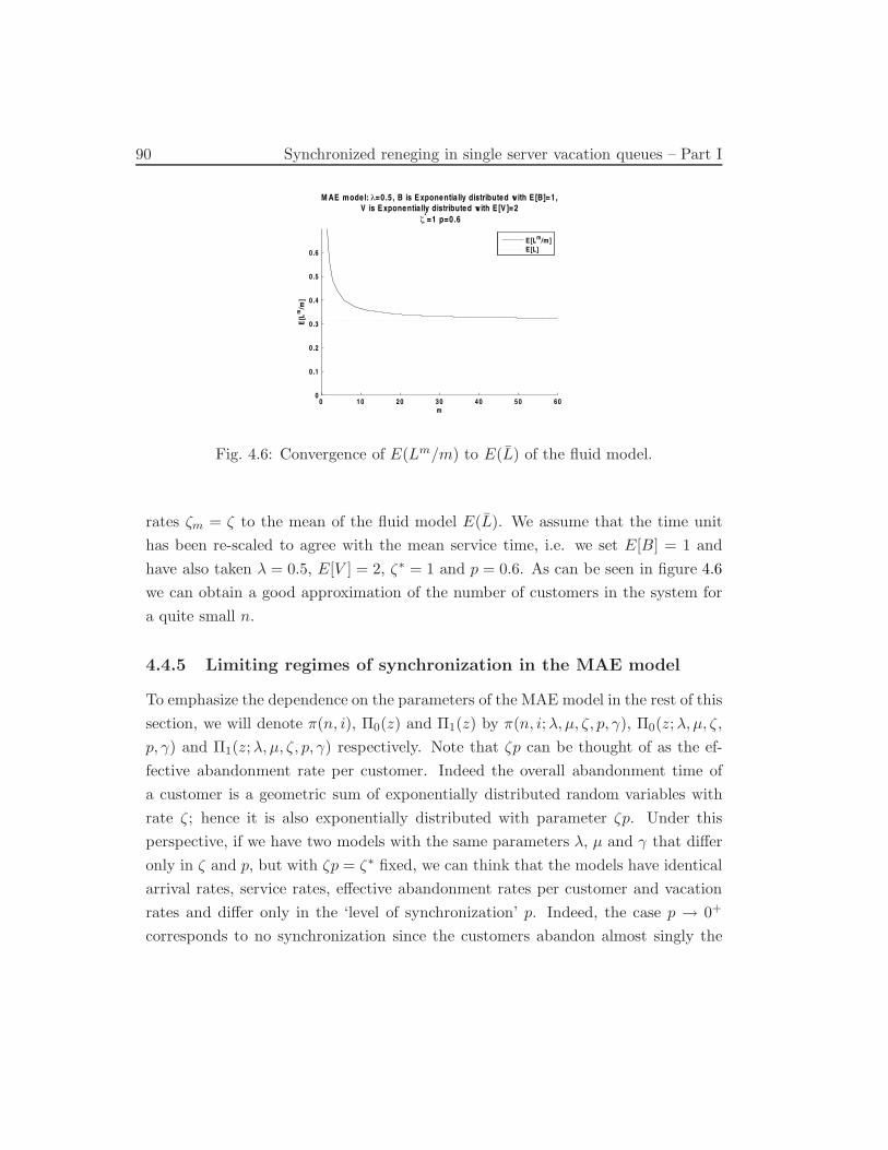
90 Synchronized reneging in single server vacation queues – Part I
0 10 20 30 40 50 600
0.1
0 .2
0 .3
0 .4
0 .5
0 .6
m
E[L
m/m
]
M AE model: λ=0.5 , B is E xponentia lly distributed with E [B]=1,V is E xponentia lly distributed with E [V ]=2
ζ*=1 p=0.6
E [Lm/m]E [L]
Fig. 4.6: Convergence of E(Lm/m) to E(L) of the fluid model.
rates +m = + to the mean of the fluid model E(L). We assume that the time unit
has been re-scaled to agree with the mean service time, i.e. we set E[B] = 1 and
have also taken " = 0.5, E[V ] = 2, +& = 1 and p = 0.6. As can be seen in figure 4.6
we can obtain a good approximation of the number of customers in the system for
a quite small n.
4.4.5 Limiting regimes of synchronization in the MAE model
To emphasize the dependence on the parameters of the MAE model in the rest of this
section, we will denote %(n, i), #0(z) and #1(z) by %(n, i;", µ, +, p, )), #0(z;", µ, +,
p, )) and #1(z;", µ, +, p, )) respectively. Note that +p can be thought of as the ef-
fective abandonment rate per customer. Indeed the overall abandonment time of
a customer is a geometric sum of exponentially distributed random variables with
rate +; hence it is also exponentially distributed with parameter +p. Under this
perspective, if we have two models with the same parameters ", µ and ) that di"er
only in + and p, but with +p = +& fixed, we can think that the models have identical
arrival rates, service rates, e"ective abandonment rates per customer and vacation
rates and di"er only in the ‘level of synchronization’ p. Indeed, the case p " 0+
corresponds to no synchronization since the customers abandon almost singly the
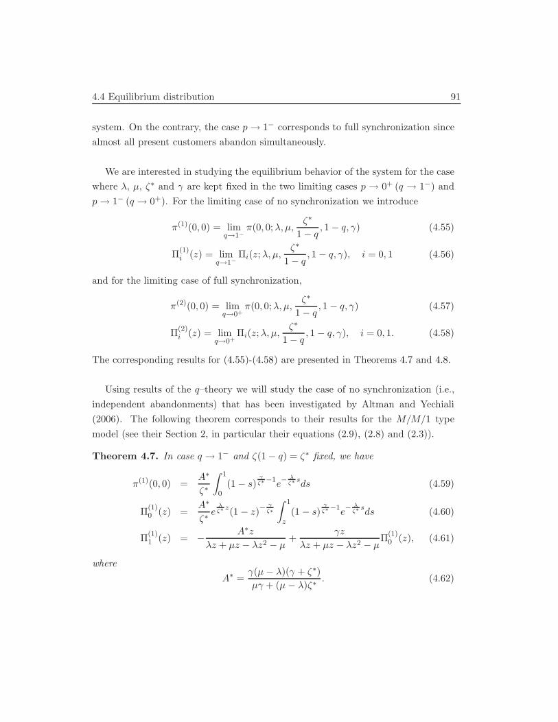
4.4 Equilibrium distribution 91
system. On the contrary, the case p " 1$ corresponds to full synchronization since
almost all present customers abandon simultaneously.
We are interested in studying the equilibrium behavior of the system for the case
where ", µ, +& and ) are kept fixed in the two limiting cases p " 0+ (q " 1$) and
p " 1$ (q " 0+). For the limiting case of no synchronization we introduce
%(1)(0, 0) = limq%1!
%(0, 0;", µ,+&
1 ! q, 1 ! q, )) (4.55)
#(1)i (z) = lim
q%1!#i(z;", µ,
+&
1 ! q, 1 ! q, )), i = 0, 1 (4.56)
and for the limiting case of full synchronization,
%(2)(0, 0) = limq%0+
%(0, 0;", µ,+&
1 ! q, 1 ! q, )) (4.57)
#(2)i (z) = lim
q%0+#i(z;", µ,
+&
1 ! q, 1 ! q, )), i = 0, 1. (4.58)
The corresponding results for (4.55)-(4.58) are presented in Theorems 4.7 and 4.8.
Using results of the q–theory we will study the case of no synchronization (i.e.,
independent abandonments) that has been investigated by Altman and Yechiali
(2006). The following theorem corresponds to their results for the M/M/1 type
model (see their Section 2, in particular their equations (2.9), (2.8) and (2.3)).
Theorem 4.7. In case q " 1$ and +(1 ! q) = +& fixed, we have
%(1)(0, 0) =A&
+&
+ 1
0(1 ! s)
"$$
$1e$!$$
sds (4.59)
#(1)0 (z) =
A&
+&e
!$$ z(1 ! z)$
"$$
+ 1
z(1 ! s)
"$$ $1e$
!$$ sds (4.60)
#(1)1 (z) = !
A&z
"z + µz ! "z2 ! µ+
)z
"z + µz ! "z2 ! µ#(1)
0 (z), (4.61)
where
A& =)(µ ! ")() + +&)
µ) + (µ ! ")+&. (4.62)
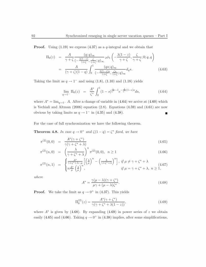
92 Synchronized reneging in single server vacation queues – Part I
Proof. Using (1.19) we express (4.37) as a q-integral and we obtain that
#0(z) =A
) + +
(q; q)#
(!"(1$z)&+) , )
&+) ; q)#2!1
.
!"(1 ! z)
) + +,
+
) + +; 0; q, q
/
=A
() + +)(1 ! q)
+ 1
0
(qs; q)#
(!"(1$z)s&+) , )s&+) ; q)#
dqs. (4.63)
Taking the limit as q " 1$ and using (1.8), (1.10) and (1.18) yields
limq%1!
#0(z) =A&
+&
+ 1
0(1 ! s)
"$$
$1e$!$$
(1$z)sds, (4.64)
where A& = limq%1! A. After a change of variable in (4.64) we arrive at (4.60) which
is Yechiali and Altman (2006) equation (2.8). Equations (4.59) and (4.61) are now
obvious by taking limits as q " 1$ in (4.35) and (4.38). !
For the case of full synchronization we have the following theorem.
Theorem 4.8. In case q " 0+ and +(1 ! q) = +& fixed, we have
%(2)(0, 0) =A&() + +&)
)() + +& + ")(4.65)
%(2)(n, 0) =
.
"
) + +& + "
/n
%(2)(0, 0), n $ 1 (4.66)
%(2)(n, 1) =
'
(
)
A$
&+)$+"$µ
%2
"µ
3n!2
"&+)$+"
3n&
, if µ (= ) + +& + "
nA$
µ
2
"µ
3n, if µ = ) + +& + ", n $ 1,
(4.67)
where
A& =)(µ ! ")() + +&)
µ) + (µ ! ")+&. (4.68)
Proof. We take the limit as q " 0+ in (4.37). This yields
#(2)0 (z) =
A&() + +&)
)() + +& + "(1 ! z)), (4.69)
where A& is given by (4.68). By expanding (4.69) in power series of z we obtain
easily (4.65) and (4.66). Taking q " 0+ in (4.38) implies, after some simplifications,
4.4 Equilibrium distribution 93
that
#(2)1 (z) =
A&"z
µ() + +& + ")(1 ! "µz)(1 ! "
&+)$+"z). (4.70)
By analyzing2
(1 ! "µz)(1 ! "
&+)$+"z)3$1
in partial fractions for the two cases µ (=) + +& + " and µ = ) + +& + ", and expanding in power series of z we obtain (4.67).
!

94 Synchronized reneging in single server vacation queues – Part I
Chapter 5
Synchronized reneging in
single server vacation queues
Part II
In this chapter we extend the analysis of the two queueing models with vacations and
impatient customers introduced in chapter 4, in a framework with general service
and vacation times.
5.1 Introduction
In this chapter, we study two models with vacations, where the customers are im-
patient but they perform synchronized abandonments. These models are motivated
by remote systems where customers have to wait for a certain transport facility to
abandon the system. Then, whenever the facility visits the system, the present cus-
tomers decide whether to leave the system or not. Therefore, we have synchronized
departures for some of the customers.
The first model is the single-server queue with multiple vacations, where cus-
tomers decide whether to abandon the system or not when the vacation periods
96 Synchronized reneging in single server vacation queues – Part II
finish. In the second model, we suppose that the abandonments epochs occur ac-
cording to a Poisson process during vacation periods. At the abandonment epochs,
every present customer remains in the system with probability q or abandons the
system with probability p = 1 ! q, independently of the others.
Chapter 5 is organized as follows. In Section 5.2, we describe the dynamics of
the models. In Section 5.3 we carry out a mean value analysis of the two models,
while in Section 5.4 we study their stationary distributions by using a generating
function approach. In Section 5.5 we present several numerical results that illustrate
the e"ect of the various parameters on the performance measures of the model.
5.2 Model description
We consider a queueing system where customers arrive one by one according to a
Poisson process at rate ". Service is provided by a single server who can be in
one of two modes: on (active) or o" (non-active - on vacation). Customers are
served singly when the server is on, while no service is provided when the server
is o". The service times are generally distributed according to a distribution B(t),
having Laplace-Stieltjes transform (LST) B(s) = E(e$sB) and finite first and second
moments E(B) and E(B2), where the random variable B represents the service time.
The residual (or equilibrium) service time is denoted by Be, the distribution Be(t)
of which is given by
Be(t) =
B t0 (1 ! B(u))du
E(B).
There is infinite waiting room. Whenever the system becomes empty, the server
begins a vacation. We assume multiple vacations, i.e., if the system is still empty
at the end of a vacation, the server takes another one. If, on the contrary, there
is at least one waiting customer at the end of a vacation, the server starts again
to provide service. The vacation times are generally distributed according to a
distribution V (t), having LST V (s) = E(e$sV ) and finite first and second moments
E(V ) and E(V 2), where the random variable V represents the vacation time. The

5.2 Model description 97
residual vacation time is denoted by Ve with distribution
Ve(t) =
B t0 (1 ! V (u))du
E(V ),
and LST
Ve(s) =1 ! V (s)
E(V )s. (5.1)
Regarding the abandonments we consider the two models that we defined in chapter
4, i.e.:
• Unique Abandonment Epoch (UAE) : Every time the server finishes a vacation,
every present customer decides whether to stay in the system with probability
q or to abandon it with probability p = 1 ! q, independently of the others.
• Multiple Abandonment Epochs (MAE) : During server vacations, abandon-
ment opportunities occur according to a Poisson process with rate +. At these
epochs, every present customer remains in the system with probability q or
abandons the system with probability p = 1 ! q, independently of the others.
Hence, in either model, the number of customers is reduced according to a bino-
mial distribution at every abandonment epoch. However, the analysis of the UAE
model turns out to be much easier than the one of the MAE model. For this reason,
in what follows, we describe briefly the results for the UAE model and we provide
more details for the analysis of the MAE model.
We are interested in the equilibrium behavior of the model, so we need to establish
first the stability condition. For the pure vacation model (p = 0) the stability
condition is (see, e.g., Takagi (1991))
, = "E(B) < 1. (5.2)
Hence, the above condition is su!cient for the stability of the UAE and MAE models.
It is also necessary, since the system behaves as a standard M/G/1 queue while the
server is active. Clearly, the only exception is the degenerate case p = 1 for the case
of the UAE model. Then condition (5.2) is not required for stability. Throughout
the paper we assume the validity of condition (5.2).
98 Synchronized reneging in single server vacation queues – Part II
5.3 Mean value analysis
We now assume the general framework introduced in Section 5.2, i.e., the service
and vacation times are both generally distributed. The analysis is similar for the two
models, so we treat them simultaneously up to the point where the abandonment
mechanism enters.
We suppose that the system is in equilibrium and we consider as before the
random variables L representing the number of customers in the system and S rep-
resenting the sojourn time of a customer. Let also Li be the conditional number of
customers in the system, given that the server is in state i, i = 0, 1. Further we
denote by pi the probability (or fraction of time) that the server is in state i, i = 0, 1.
Let us consider a tagged arriving customer. Then, by PASTA, the probability that
this customer finds the server in state i is pi and in this case, he finds on average
E(Li) customers in front of him.
If he finds the server providing service, then his mean sojourn time is equal to
the residual service time of the customer in service plus the service times of all cus-
tomers waiting in the queue plus his own service time. Hence, his mean sojourn
time is E(Be) + (E(L1) ! 1)E(B) + E(B).
If he finds the server on vacation, then he has to wait for the vacation time to
expire before servicing starts and he may decide to abandon at one of the abandon-
ment opportunities (there is just one in case of the UAE model, but possibly many
in case of the MAE model). Let E(V &) be his mean time in the system till the end
of the vacation. If the tagged customer is still in the system just after the end of
the vacation, then his sojourn time after the return of the server depends on the
number of customers (still) in front of him. Define % as the probability that the
tagged customer stays in the system at the end of the vacation period and define
%& as the probability that the tagged customer and a customer, who was already
present at his arrival, both stay in the system. Then, we have that the mean number
5.3 Mean value analysis 99
of customers in front of him at the end of the vacation period is %&E(L0). Hence
E(S) = p1 (E(Be) + E(L1)E(B)) + p0 (E(V &) + %&E(L0)E(B) + %E(B)) . (5.3)
Further, Little’s law states that
E(L) = "E(S). (5.4)
Also, if we would act as if the customers arriving during a vacation are waiting in
a “vacation area” and transferred to the queue as soon as the server returns, then
application of Little’s law to the vacation area yields
E(L0) = "E(V &). (5.5)
The unconditional E(L) is related to the conditional ones as
E(L) = p0E(L0) + p1E(L1). (5.6)
Conservation of work gives
p1 = ("p0% + "p1)E(B), (5.7)
and,
p0 + p1 = 1. (5.8)
If we determine %, then the equations (5.7)-(5.8) yield immediately the probabilities
p0 and p1. If we also determine %& and E(V &), then the equations (5.3)-(5.6) su!ce
for the computation of the unknown mean values E(L), E(L0), E(L1) and E(S). The
computations of %, %& and E(V &) depend on the specific abandonment mechanism,
so we treat the UAE and the MAE models separately.
5.3.1 Mean value analysis of the UAE model
In the UAE model a customer that arrives when the server is on vacation has a
unique opportunity to abandon the system at the end of the vacation. Therefore
he will stay in the system for the residual vacation time and then he will decide
100 Synchronized reneging in single server vacation queues – Part II
whether to leave or not, so E(V &) = E(Ve). The probability % is clearly equal to q,
while %& is equal to q2. Solution of (5.3)-(5.8) yields:
Theorem 5.1. The mean sojourn time is given by
E(S) =1
1 ! ,p
,
E(Ve) + (q2 ! 1),E(Ve)-
+q
1 ! ,p
.
,E(Be)
1 ! ,+ E(B)
/
,
and the fraction of time the server is inactive and active, respectively,
p0 =1 ! ,
1 ! ,p, p1 =
,q
1 ! ,p. (5.9)
5.3.2 Mean value analysis of the MAE model
In the MAE model a customer that arrives when the server is on vacation may
have several opportunities to abandon the system. The computation of %, %& and
E(V &) is not immediate as in case of the UAE model. However, we observe that,
if the tagged customer arrives during a vacation, then the time till abandonment
is exponential with rate +p. By denoting the time till abandonment by T , we can
write
V & = min(Ve, T ) and % = P (Ve < T ).
Hence, by conditioning on the length of Ve,
% =
+ #
0P (t < T )dVe(t)
=
+ #
0e$)ptdVe(t)
= Ve(+p), (5.10)
and
E(V &) = E(Ve + T ) ! E(max(Ve, T ))
= E(Ve) +1
+p!.
E(Ve) + %1
+p
/
= (1 ! %)1
+p. (5.11)
5.4 Equilibrium distribution 101
To compute %& we condition on the length of Ve and on the number of abandonment
epochs during Ve,
%& =
+ #
0
#$
n=0
e$)t(+t)n
n!(q2)ndP (Ve & t)
=
+ #
0e$)te)tq
2dVe(t)
=
+ #
0e$)(1$q2)tdVe(t)
= Ve(+(1 ! q2)). (5.12)
By solving (5.3)-(5.8), and taking into account (5.10)-(5.12), we finally get:
Theorem 5.2. The mean sojourn time is equal to
E(S) =1
1 ! , + ,%(E(V &) + (%& ! 1),E(V &)) +
%
1 ! , + ,%
.
,E(Be)
1 ! ,+ E(B)
/
,
where %, %& and E(V &) are given by (5.10), (5.12) and (5.11), respectively, and
p0 =1 ! ,
1 ! , + ,%, p1 =
,%
1 ! , + ,%. (5.13)
5.4 Equilibrium distribution
The aim of this section is to determine the PGF of the number of customers in the
system. By conditioning on the state of the server, we obtain
E(zL) = p0E(zL0) + p1E(zL1). (5.14)
On what the PGF of L1 is concerned we have the following theorem.
Theorem 5.3. The PGF of L1 can be obtained as
E(zL1) =(1 ! ,)
,·z(1 ! B("(1 ! z)))
B("(1 ! z)) ! z·
1 ! E(zLv )
E(Lv)(1 ! z), (5.15)
where Lv denotes the number of customers in the system just after the end of the
vacation.
102 Synchronized reneging in single server vacation queues – Part II
We will provide three separate proofs for theorem 5.3 because each one of them
reveals a new probabilistic viewpoint for studying the system under consideration.
The first one is more intuitive while the other two use strict probabilistic arguments
from the theory of regenerative processes.
Proof I. To find the PGF of L1 we first need the number of customers in the system
just after the end of a vacation which we have denoted by Lv. We now proceed as in
Fuhrmann (1984). Define the primary customers to be the ones just after the start
of the busy period and the secondary customers to be the ones who arrive during
the busy period. Further, we change the service discipline to non-preemptive LCFS;
this does not a"ect the number of customers in the system. So, after servicing a
primary customer, the server will serve any secondary customer until there is none
present. Each primary customer generates a standard M/G/1 busy period, at the
end of which the server either begins servicing the next primary customer or, if the
system is empty, takes a vacation. Let Qp be the number of primary customers
waiting for service in the queue (excluding the one possibly in service). If we remove
server vacations from the time axis and glue together the service periods, then we
readily obtain from the renewal reward theorem (see, e.g., Ross (2003)) that the
fraction of time the queue contains n primary customers is equal to
P (Qp = n) =P (Lv > n)
E(Lv), n $ 0.
Hence,
E(zQp) =1
E(Lv)
#$
n=0
P (Lv > n)zn =1 ! E(zLv )
E(Lv)(1 ! z). (5.16)
Let L1|M/G/1 denote the conditional number of customers in the corresponding stan-
dard M/G/1 with arrival rate " and service time distribution B(t), given that the
server is in state 1 (i.e., active); so, according to the Pollaczek-Khinchin formula,
E(zL1|M/G/1) =(1 ! ,)
,·z(1 ! B("(1 ! z)))
B("(1 ! z)) ! z. (5.17)
Since L1 = L1|M/G/1 + Qp, where L1|M/G/1 and Qp are independent, we obtain, by
(5.16) and (5.17),
E(zL1) = E(zL1|M/G/1)E(zQp), (5.18)

5.4 Equilibrium distribution 103
which concludes the proof of theorem 5.3. !
Proof II. Let %j be the fraction of time spent in state j during a busy period.
Then %j = E["j]E["] , where %j denotes the time spent in state j during a busy period
and % the length of the busy period. The r.v. Lv denotes the number of customers
just after the end of the vacation time, with corresponding PGF E[zLv ]. The server
starts to serve when Lv customers have been accumulated in the system. Therefore
the mean length of the busy period for this system is equal to E[Lv ] ·E[&], where &
is the duration of the busy period for the M/G/1 queue. More explicitly
E[%] = E[Lv ]E[&] = E[Lv]E[B]
1 ! ,
= E[Lv ]1
"
,
1 ! ,. (5.19)
Let &j denote the time spent in state j during a busy period for the M/G/1 queue.
Given Lv = n, we can easily obtain that
E[%j |Lv = n] =j$
k=1
E[&k] , j < n, (5.20)
since the time spent in state j given that Lv = n > j is equal to the time spent in
j starting from state j until the first time that the system visits j ! 1 + the time
spent in j from j ! 1 to j ! 2 + · · · + the time spent in j from 1 to 0 which is equal
to the time spent in state 1 in the M/G/1 queue in one cycle + the time spent in
state 2 in the M/G/1 queue in one cycle + · · · + the time spent in state j in the
M/G/1 queue in one cycle. Similarly, when Lv = n & j we obtain,
E[%j |Lv = n] =n$
k=1
E[&j$n+k] , j $ n. (5.21)
Therefore
E[%j |Lv = n] = 1{j<n}
j$
k=1
E[&k] + 1{j'n}
n$
k=1
E[&j$n+k] . (5.22)
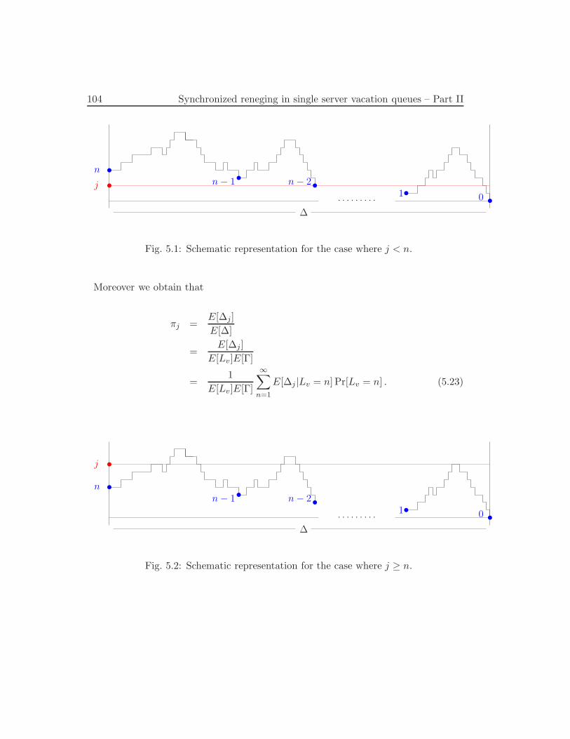
104 Synchronized reneging in single server vacation queues – Part II
. . . . . . . . .
!
!n
!j!
n ! 1 !n ! 2!1
!0
Fig. 5.1: Schematic representation for the case where j < n.
Moreover we obtain that
%j =E[%j]
E[%]
=E[%j]
E[Lv]E[&]
=1
E[Lv]E[&]
#$
n=1
E[%j |Lv = n] Pr[Lv = n] . (5.23)
. . . . . . . . .
!
!n
!j
!
n ! 1 !n ! 2!1
!0
Fig. 5.2: Schematic representation for the case where j $ n.
5.4 Equilibrium distribution 105
By plugging (5.22) in (5.23) we obtain
%j =1
E[Lv]
#$
n=1
j$
k=1
E[&k]
E[&]Pr[Lv = n]1{j<n}
+1
E[Lv]
#$
n=1
n$
k=1
E[&j$n+k]
E[&]Pr[Lv = n]1{j'n} . (5.24)
We define pk to be the steady state probabilities of the M/G/1 queue and E[zLM/G/1 ]
the corresponding PGF. But E[#j ]E[#] = pj
1$p0- E[&j ] = pj
E[#]* . Equation (5.24),
then, assumes the form
%j =1
,E[Lv ]
#$
n=1
j$
k=1
pk Pr[Lv = n]1{j<n}+1
,E[Lv]
#$
n=1
n$
k=1
pj$n+k Pr[Lv = n]1{j'n} .
(5.25)
Then the PGF E[zL1 ] takes the following form
E[zL1 ] =#$
j=1
%jzj
(5.25)=
1
,E[Lv]
#$
j=1
zj#$
n=1
j$
k=1
pk Pr[Lv = n]1{j<n}
+1
,E[Lv]
#$
j=1
zj#$
n=1
n$
k=1
pj$n+k Pr[Lv = n]1{j'n}
=1
,E[Lv]
#$
n=1
n$1$
j=1
zjj$
k=1
pk Pr[Lv = n]
+1
,E[Lv]
#$
n=1
#$
j=n
zjn$
k=1
pj$n+k Pr[Lv = n]
=1
,E[Lv]
#$
n=1
;
=
#$
j=1
zjj$
k=1
pk !#$
j=n
zjj$
k=1
pk
+#$
j=n
zjj$
k=j$n+1
pk
>
@Pr[Lv = n]
106 Synchronized reneging in single server vacation queues – Part II
=1
,E[Lv]
#$
n=1
;
=
#$
j=1
zjj$
k=1
pk !#$
j=n
zjj$n$
k=1
pk
>
@Pr[Lv = n]
=1
,E[Lv]
#$
n=1
;
=
#$
j=1
zjj$
k=1
pk ! zn#$
j=1
zjj$
k=1
pk
>
@Pr[Lv = n]
=1
,E[Lv]
#$
n=1
Pr[Lv = n](1 ! zn)#$
k=1
pk
#$
j=k
zj
=1
,E[Lv]
#$
n=1
Pr[Lv = n](1 ! zn)#$
k=1
pkzk
1 ! z
=1
,E[Lv]
#$
n=1
Pr[Lv = n]1 ! zn
1 ! z(E[zLM/G/1 ] ! p0)
=(E[zLM/G/1 ] ! p0)
,E[Lv ]
1 ! E[zLv ]
1 ! z. (5.26)
Using that E[zLM/G/1 ] = p0(1$z)B("(1$z))
B("(1$z))$zand p0 = 1 ! , in equation (5.26) yields
(5.15). !
Proof III. Following the notation that was introduced in proof II we will now
divide a cycle into a random number of disjoint intervals separated by the service
completion epochs and calculate E[%j ] as the sum of the contributions from the
disjoint intervals to the expected sojourn time in state j. Thus we define the random
variables Nj by
Nj = the number of service completion epochs in one cycle at which j cus-
tomers are left behind, j = 0, 1, . . ..
Moreover, using the lack of memory of the Poisson arrival process, we define the
quantity Akj by
Akj = the expected amount of time that j customers are present during a
service time starting when k customers are present.
Then, given that Lv = n, we note that the first service in a cycle starts with n
5.4 Equilibrium distribution 107
customers, it follows that
E[%j |Lv = n] = Anj +j$
k=1
E[Nk|Lv = n]Akj , j = n, n + 1, . . . (5.27)
while for all states j < n we observe that they can’t be reached during the first
service and so
E[%j |Lv = n] =j$
k=1
E[Nk|Lv = n]Akj , j = 1, 2, . . . , n ! 1 . (5.28)
In general
E[%j |Lv = n] = Anj1{j'n} +j$
k=1
E[Nk|Lv = n]Akj , j = 1, 2, . . . . (5.29)
We can obtain a relation between E[%j |Lv = n] and E[Nj |Lv = n], using a simple
observation that given Lv = n
the number of downcrossings from state j + 1 to j in one cycle
= the number of upcrossings from state j to j + 1 in one cycle, for all j =
n, n + 1, . . . ,
the number of downcrossings from state j + 1 to j in one cycle
= the number of upcrossings from state j to j + 1 in one cycle + 1, for all
j = 1, 2, . . . , n ! 1 .
The expected number of downcrossings from state j +1 to j in one cycle, given that
Lv = n, is by definition equal to E[Nj |Lv = n]. On the other hand, since the arrival
process is a Poisson process, we have that the expected number of upcrossing from
state j to j + 1 in one cycle, given that Lv = n, is equal to "E[%j |Lv = n]. Thus
we find
E[Nj |Lv = n] = 1{j<n} + "E[%j|Lv = n], j = 1, 2, . . . . (5.30)
Substituting equation (5.30) into equation (5.29) we obtain that
E[%j |Lv = n] = Anj1{j'n}+j$
k=1
Akj1{k<n}+"j$
k=1
E[%k|Lv = n]Akj , j = 1, 2, . . . .
(5.31)
108 Synchronized reneging in single server vacation queues – Part II
Then
E[%j ] =#$
n=1
E[%j |Lv = n] Pr[Lv = n]
=#$
n=1
Anj1{j'n} Pr[Lv = n] +#$
n=1
j$
k=1
Akj1{k<n} Pr[Lv = n]
+"#$
n=1
j$
k=1
E[%k|Lv = n]Akj Pr[Lv = n]
=#$
n=1
Anj1{j'n} Pr[Lv = n] +#$
n=1
j$
k=1
Akj1{k<n} Pr[Lv = n]
+"j$
k=1
E[%k]Akj . (5.32)
Dividing both sides of equation (5.32) by E[%] we obtain
%j =1
E[%]
#$
n=1
Anj1{j'n} Pr[Lv = n] +1
E[%]
#$
n=1
j$
k=1
Akj1{k<n} Pr[Lv = n]
+"j$
k=1
%kAkj . (5.33)
To specify the constants Akj, suppose that at epoch 0 a service starts when k
customers are present. Define the random variable Ij(t) = 1 if at time t the service
is still in progress and j customers are present and let Ij(t) = 0 otherwise. Then for
j $ k,
Akj = E[
+ #
0Ij(t)dt]
=
+ #
0Pr[Ij(t) = 1]dt]
=
+ #
0Pr[B $ t]e$"t
("t)j$k
(j ! k)!dt
=
+ #
0(1 ! B(t))e$"t
("t)j$k
(j ! k)!dt . (5.34)
5.4 Equilibrium distribution 109
Let Akj = aj$k and let A(z) =!#
n=0 anzn be the corresponding PGF, then
A(z) =#$
n=0
zn+ #
0(1 ! B(t))e$"t
("t)n
n!dt
=
+ #
0(1 ! B(t))e$"t
#$
n=0
("tz)n
n!dt
=
+ #
0(1 ! B(t))e$"(1$z)tdt
=1 ! B("(1 ! z))
"(1 ! z). (5.35)
We define the generating function E[zL1 ] by
E[zL1 ] =#$
j=1
%jzj , |z| & 1 .
Multiplying both sides of (5.33) by zj and summing over j we derive that
E[zL1 ] =1
E[%]
,
A(z)E[zLv ] + A(z)z1 ! E[zLv ]1z
1 ! z
-
+ "E[zL1 ]A(z) . (5.36)
Solving for E[zL1 ] and substituting equations (5.19) and (5.35) yields (5.15). !
It is now clear that the determination of the PGF of the number of customers
in the system reduces to the computation of E(zL0), E(zLv ) and E(Lv). These
computations depend on the specific abandonment mechanism, so we treat the UAE
and the MAE model separately.
5.4.1 Equilibrium distribution of the UAE model
In this case the probabilities p0 and p1 are given by (5.9). The number of customers
during a vacation, L0, are exactly the ones who arrived during the age of the va-
cation, and the age is in distribution the same as the residual vacation. Hence, by
conditioning on Ve = t, the number of arrivals is Poisson with parameter "t, and
110 Synchronized reneging in single server vacation queues – Part II
thus we get
E(zL0) =
+ #
0e$"t(1$z)dVe(t)
= Ve("(1 ! z)). (5.37)
The number of arrivals during a vacation of length t, who decide to stay at the end
of the vacation, is Poisson with parameter q"t. Hence, the PGF of the number of
customers in the system, just after the end of the vacation, is
E(zLv ) = V (q"(1 ! z)). (5.38)
We can now combine (5.14), (5.15), (5.37), (5.38) and (5.1) to obtain the PGF
of the number of customers in the system. We have the following theorem.
Theorem 5.4. The PGF of the number of customers in the system is given by
E(zL) =1 ! ,
1 ! ,pVe("(1 ! z)) +
q(1 ! ,)
1 ! ,p
z(1 ! B("(1 ! z)))
B("(1 ! z)) ! zVe(q"(1 ! z)).
Remark 5.1. In case q = 1 ! p = 1, the equation above reduces to the well-known
Fuhrmann-Cooper decomposition for the number of customers in the M/G/1 with
server vacations (and no abandonments),
E(zL) = Ve("(1 ! z))E(zLM/G/1), (5.39)
where LM/G/1 is the (unconditional) number of customers in the corresponding
standard M/G/1.
5.4.2 Equilibrium distribution of the MAE model
In this case the probabilities p0 and p1 are given by (5.13). We need also to ob-
tain E(zL0), E(zLv ) and E(Lv). We start with the latter. Conditioning on the
event that V = t, the number of abandonment epochs is Poisson with parameter +t.
Given the number of abandonment epochs is n(> 0), the event times (s1, s2, . . . , sn)
of these epochs will be distributed as the order statistics (U1:n, U2:n, . . . , Un:n) of a
random sample (U1, U2, . . . , Un) from the uniform distribution in (0, t]. The number
5.4 Equilibrium distribution 111
of arrivals in each of the intervals (0, s1], (s1, s2], . . ., (sn$1, sn], (sn, t] are Poisson
with parameters "s1, "(s2 ! s1), . . ., "(sn ! sn$1), "(t! sn) respectively. Moreover,
the individuals that arrive during these intervals with remain till time t with prob-
abilities qn, qn$1, . . ., q, 1 respectively. Since the sum of Poisson random variables
is again Poisson, we can conclude that the number of customers at the end of the
vacation is Poisson with parameter
'(t, n, s1, . . . , sn) = "s1qn + "(s2 ! s1)q
n$1 + · · · + "(sn ! sn$1)q + "(t ! sn)
= !"qn$1(1 ! q)s1 ! "qn$2(1 ! q)s2 ! · · ·! "(1 ! q)sn + "t,
valid for n > 0, and if n = 0, this number is Poisson with parameter "t. Hence,
E(zLv |V = t) = e$)te$"t(1$z)
+#$
n=1
+ t
0
+ t
s1
· · ·+ t
sn!1
e$)t(+t)n
n!e$$(t,n,s1,...,sn)(1$z) n!
tndsn · · · ds1 .
(5.40)
To put E(zLv |V = t) in a more compact form, we use the auxiliary identity
In(t, n,*1,*2, . . . ,*n) =
+ t
0
+ t
s1
· · ·+ t
sn!1
e+1s1++2s2+···++nsndsn · · · ds2ds1
=n+1$
k=1
(!1)k+1etPn
i=k +i
6n$ki=0
!k+ij=k *j ·
6k$1i=1
!k$1j=k$i *j
, (5.41)
which can be easily established by induction. In order to use (5.41) to simplify (5.40)
we substitute
*j = "(1 ! q)(1 ! z)qn$j , j = 1, 2, . . . , n (5.42)
112 Synchronized reneging in single server vacation queues – Part II
andn$
i=k
*i = "(1 ! z)(1 ! qn$k+1) (5.43)
k+i$
j=k
*j = "(1 ! z)(1 ! qi+1)qn$k$i (5.44)
k$1$
j=k$i
*j = "(1 ! z)qn$k+1(1 ! qi) (5.45)
n$k*
i=0
k+i$
j=k
*j = ["(1 ! z)]n$k+1q(n!k+1
2 )(q; q)n$k+1 (5.46)
k$1*
i=1
k$1$
j=k$i
*j = ["(1 ! z)]k$1q(n$k+1)(k$1)(q; q)k$1. (5.47)
in (5.41), yielding (after some algebra)
In(t, n,*1,*2, . . . ,*n) =et"(1$z)
["(1 ! z)]n
n$
k=0
(!1)ke$t"(1$z)qn!k
(q; q)k(q; q)n$kq(n!k
2 )+(n$k)k. (5.48)
Using (5.40), (5.41) and (5.48) we obtain
E(zLv |V = t) = e$()+"(1$z))t#$
n=0
+nn$
k=0
et"(1$z)(1$qn!k)
("(1 ! z))n(!1)kq$(n+k$1)(n$k)/2
(q; q)k(q; q)n$k
= e$)t#$
n=0
.
+
"(1 ! z)
/n n$
k=0
(!1)kq$(n+k$1)(n$k)/2
(q; q)k(q; q)n$ke$t"(1$z)qn!k
= e$)t#$
k=0
(!1)k
(q; q)k
#$
n=k
.
+
"(1 ! z)
/n q$(n+k$1)(n$k)/2
(q; q)n$ke$t"(1$z)qn!k
= e$)t#$
k=0
(!1)k
(q; q)k
#$
n=0
.
+
"(1 ! z)
/n+k q$(n+2k$1)n/2
(q; q)ne$t"(1$z)qn
= e$)t#$
n=0
.
+
"(1 ! z)
/n q$(n2)
(q; q)ne$t"(1$z)qn
#$
k=0
1
(q; q)k
.
!+q$n
"(1 ! z)
/k
= e$)t#$
n=0
.
+
"(1 ! z)
/n q$(n2)
(q; q)ne$t"(1$z)qn 1
(! )q!n
"(1$z) ; q)#
5.4 Equilibrium distribution 113
= e$)t#$
n=0
.
+
"(1 ! z)
/n q$(n2)
(q; q)ne$t"(1$z)qn
)1
2
)"(1$z)
3nq$(n
2)$n(!"(1$z)q) ; q)n(! )
"(1$z) ; q)#
=e$)t
(! )"(1$z) ; q)#
#$
n=0
qne$t"(1$z)qn
(q; q)n(!"(1$z)q) ; q)n
. (5.49)
Hence, after unconditioning, we conclude that the PGF of Lv assumes the form
E(zLv ) =
+ #
0E(zLv |V = t)dV (t)
=
+ #
0
e$)t
(! )"(1$z) ; q)#
#$
n=0
qn
(q; q)ne$t"(1$z)qn 1
(!"(1$z)q) ; q)n
dV (t)
=1
(! )"(1$z) ; q)#
#$
n=0
qnV (+ + "(1 ! z)qn)
(q; q)n(!"(1$z)q) ; q)n
. (5.50)
Moreover,
E(Lv|V = t) = e$)t"t
+#$
n=1
+ t
0
+ t
s1
· · ·+ t
sn!1
e$)t(+t)n
n!'(t, n, s1, . . . , sn)
n!
tndsn · · · ds1.
(5.51)
To put E(Lv |V = t) in a more compact form we use the auxiliary identity
Jn(t, n,*1,*2, . . . ,*n) =
+ t
0
+ t
s1
· · ·+ t
sn!1
[*0 + *1s1 + · · · + *nsn] dsn · · · ds2ds1
= *0tn
n!+
n$
k=1
*kk tn+1
(n + 1)!, (5.52)
which can be easily established by induction. In order to use (5.52) to simplify (5.51)
we substitute
*0 = "t
*j = !"(1 ! q)qn$j, j = 1, 2, . . . , n
114 Synchronized reneging in single server vacation queues – Part II
in (5.52), yielding
Jn(t, n,*1,*2, . . . ,*n) = "tn+1
(n + 1)!
1 ! qn+1
1 ! q. (5.53)
Using (5.51) and (5.53) we obtain
E(Lv|V = t) ="
+p(1 ! e$)pt). (5.54)
Note that, after unconditioning, the mean value of Lv assumes the form
E(Lv) ="
+p(1 ! V (+p)). (5.55)
To determine the PGF of the number of customers during a vacation, we can copy
the approach above, where the vacation V should be replaced by its age Ve. This
leads to
E(zL0) =
+ #
0E(zL0 |Ve = t)dVe(t)
=
+ #
0
e$)t
(! )"(1$z) ; q)#
#$
n=0
qn
(q; q)ne$t"(1$z)qn 1
(!"(1$z)q) ; q)n
dVe(t)
=1
(! )"(1$z) ; q)#
#$
n=0
qnVe(+ + "(1 ! z)qn)
(q; q)n(!"(1$z)q) ; q)n
. (5.56)
Based on the PGFs of L0, Lv and the mean value E(Lv) we can now use (5.14),
(5.15), (5.56) and (5.50) to obtain the PGF of the number of customers in the
system. Therefore, we immediately obtain the following result.
Theorem 5.5. The PGF of the number of customers in the system is given by
E(zL) =1 ! ,
1 ! , + ,%E(zL0)+
%(1 ! ,)
1 ! , + ,%
z(1 ! B("(1 ! z)))
B("(1 ! z)) ! z
1 ! E(zLv )
E(Lv)(1 ! z), (5.57)
where %, E(zL0), E(zLv ) and E(Lv) are given by (5.10), (5.56), (5.50) and (5.55),
respectively.
5.5 Numerical results 115
Remark 5.2. As the rate + of the abandonment epochs tends to zero (i.e., no
abandonments), then equation (5.57) again reduces to the standard decomposition
(5.39). To show this, we first use the identity
(a; q)n = (a$1q1$n; q)n(!a)nq(n2)
to rewrite (5.50) in the form
E(zLv ) =#$
n=0
+n
("(1 ! z))nV (+ + "(1 ! z)qn)
(q; q)n(! )q!n
"(1$z) ; q)#q(n2)
.
For + = 0 this equation reduces to E(zLv ) = V ("(1! z)). Similarly, it can be shown
that E(zL0) = Ve("(1 ! z)) for + = 0. Substitution of these expressions into (5.57)
yields (5.39).
5.5 Numerical results
This section is devoted to several numerical results that shed further light on the
e"ect of the various model parameters and distributions on the system performance.
To this end we perform several numerical experiments by keeping all but one pa-
rameter fixed and study the mean number of customers in the system as a function
of the varying parameter. The e"ect of ", E(B) or E(V ) on the mean number
of customers in the system, E(L), appears to be what is normally expected, i.e.,
E(L) is increasing in ", E(B) and E(V ). Much more interesting is the e"ect of the
abandonment probability p on E(L). In the numerical scenarios presented below
we assume that B is exponentially distributed with E(B) = 1, and to show the
e"ect of the dispersion of the vacation times, we consider Erlang, exponential and
Hyper-exponential vacation time distributions.
We present the results for the UAE and the MAE model separately, as they are
qualitatively di"erent.
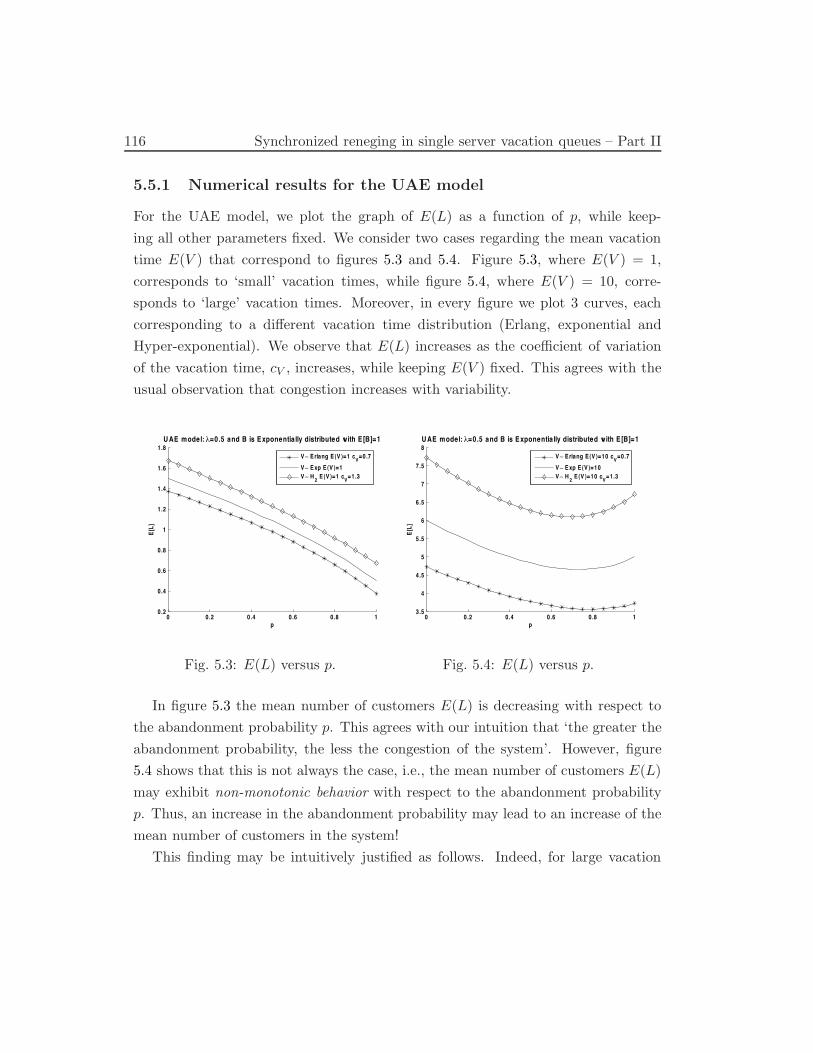
116 Synchronized reneging in single server vacation queues – Part II
5.5.1 Numerical results for the UAE model
For the UAE model, we plot the graph of E(L) as a function of p, while keep-
ing all other parameters fixed. We consider two cases regarding the mean vacation
time E(V ) that correspond to figures 5.3 and 5.4. Figure 5.3, where E(V ) = 1,
corresponds to ‘small’ vacation times, while figure 5.4, where E(V ) = 10, corre-
sponds to ‘large’ vacation times. Moreover, in every figure we plot 3 curves, each
corresponding to a di"erent vacation time distribution (Erlang, exponential and
Hyper-exponential). We observe that E(L) increases as the coe!cient of variation
of the vacation time, cV , increases, while keeping E(V ) fixed. This agrees with the
usual observation that congestion increases with variability.
0 0.2 0 .4 0 .6 0 .8 10.2
0 .4
0 .6
0 .8
1
1.2
1 .4
1 .6
1 .8
p
E[L
]
U AE model: λ=0.5 and B is E xponentia lly distributed with E [B]=1
V∼ E rlang E (V )=1 c
V=0.7
V∼ E xp E (V )=1V∼ H
2 E (V )=1 c
V=1.3
Fig. 5.3: E(L) versus p.
0 0.2 0 .4 0 .6 0 .8 13.5
4
4.5
5
5.5
6
6.5
7
7.5
8
p
E[L
]
U AE model: λ=0.5 and B is E xponentia lly distributed with E [B]=1
V∼ E rlang E (V )=10 c
V=0.7
V∼ E xp E (V )=10V∼ H
2 E (V )=10 c
V=1.3
Fig. 5.4: E(L) versus p.
In figure 5.3 the mean number of customers E(L) is decreasing with respect to
the abandonment probability p. This agrees with our intuition that ‘the greater the
abandonment probability, the less the congestion of the system’. However, figure
5.4 shows that this is not always the case, i.e., the mean number of customers E(L)
may exhibit non-monotonic behavior with respect to the abandonment probability
p. Thus, an increase in the abandonment probability may lead to an increase of the
mean number of customers in the system!
This finding may be intuitively justified as follows. Indeed, for large vacation
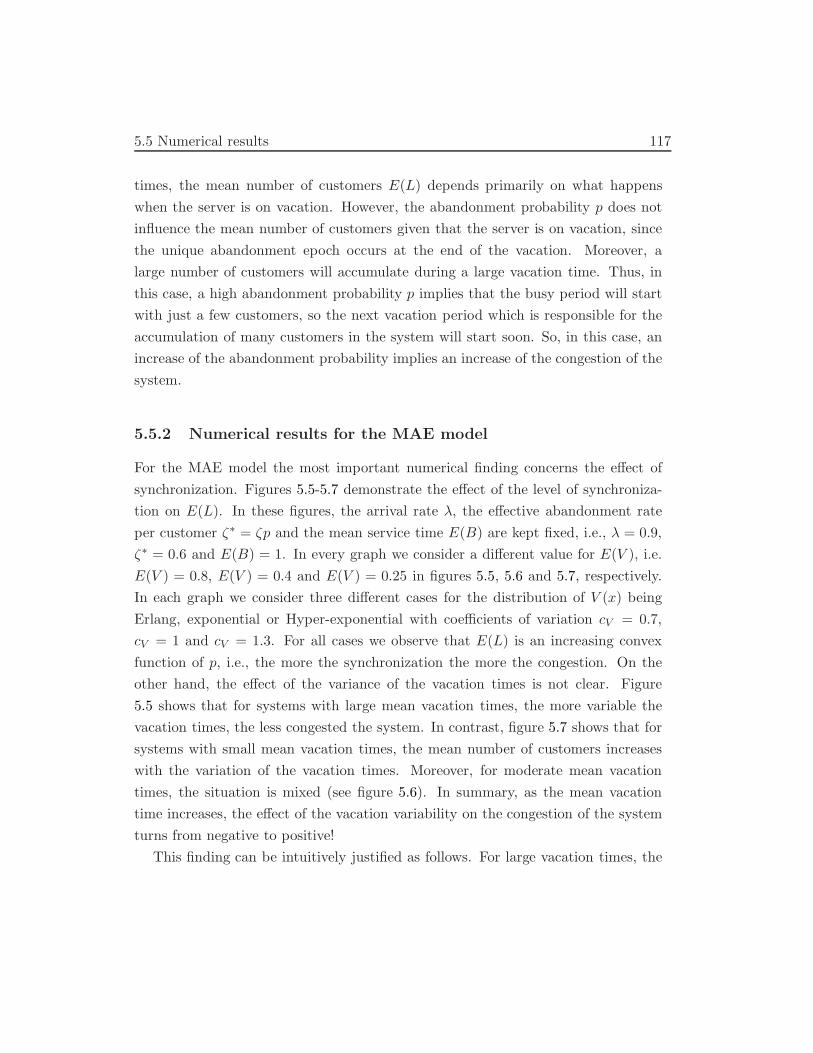
5.5 Numerical results 117
times, the mean number of customers E(L) depends primarily on what happens
when the server is on vacation. However, the abandonment probability p does not
influence the mean number of customers given that the server is on vacation, since
the unique abandonment epoch occurs at the end of the vacation. Moreover, a
large number of customers will accumulate during a large vacation time. Thus, in
this case, a high abandonment probability p implies that the busy period will start
with just a few customers, so the next vacation period which is responsible for the
accumulation of many customers in the system will start soon. So, in this case, an
increase of the abandonment probability implies an increase of the congestion of the
system.
5.5.2 Numerical results for the MAE model
For the MAE model the most important numerical finding concerns the e"ect of
synchronization. Figures 5.5-5.7 demonstrate the e"ect of the level of synchroniza-
tion on E(L). In these figures, the arrival rate ", the e"ective abandonment rate
per customer +& = +p and the mean service time E(B) are kept fixed, i.e., " = 0.9,
+& = 0.6 and E(B) = 1. In every graph we consider a di"erent value for E(V ), i.e.
E(V ) = 0.8, E(V ) = 0.4 and E(V ) = 0.25 in figures 5.5, 5.6 and 5.7, respectively.
In each graph we consider three di"erent cases for the distribution of V (x) being
Erlang, exponential or Hyper-exponential with coe!cients of variation cV = 0.7,
cV = 1 and cV = 1.3. For all cases we observe that E(L) is an increasing convex
function of p, i.e., the more the synchronization the more the congestion. On the
other hand, the e"ect of the variance of the vacation times is not clear. Figure
5.5 shows that for systems with large mean vacation times, the more variable the
vacation times, the less congested the system. In contrast, figure 5.7 shows that for
systems with small mean vacation times, the mean number of customers increases
with the variation of the vacation times. Moreover, for moderate mean vacation
times, the situation is mixed (see figure 5.6). In summary, as the mean vacation
time increases, the e"ect of the vacation variability on the congestion of the system
turns from negative to positive!
This finding can be intuitively justified as follows. For large vacation times, the

118 Synchronized reneging in single server vacation queues – Part II
0 0.1 0 .2 0 .3 0 .4 0 .5 0 .6 0 .7 0 .8 0 .9 18.92
8.94
8.96
8.98
9
9.02
9.04
9.06
9.08
9.1
p
E[L
]
M AE model: λ=0.9 , ζ*=0 .6 , B is E xponentia lly distributed with E [B]=1
V∼ E rlang E (V )=0 .8 cV
=0.7
V∼ E xp E (V )=0 .8V∼ H
2 E (V )=0 .8 c
V=1.3
Fig. 5.5: E(L) versus p, +& fixed.
0 0.1 0 .2 0 .3 0 .4 0 .5 0 .6 0 .7 0 .8 0 .9 19.02
9.03
9.04
9.05
9.06
9.07
9.08
9.09
pE
[L]
M AE model: λ=0.9 , ζ*=0 .6 , B is E xponentia lly distributed with E [B]=1
V∼ E rlang E (V )=0 .4 cV
=0.7
V∼ E xp E (V )=0 .4V∼ H
2 E (V )=0 .4 c
V=1.3
Fig. 5.6: E(L) versus p, +& fixed.
0 0.1 0 .2 0 .3 0 .4 0 .5 0 .6 0 .7 0 .8 0 .9 19.035
9.04
9.045
9.05
9.055
9.06
9.065
9.07
9.075
p
E[L
]
M AE model: λ=0.9 , ζ*=0 .6 , B is E xponentia lly distributed with E [B]=1
V∼ E rlang E (V )=0 .25 cV
=0.7
V∼ E xp E (V )=0 .25V∼ H
2 E (V )=0 .25 c
V=1.3
Fig. 5.7: E(L) versus p, +& fixed.
0 0.1 0 .2 0 .3 0 .4 0 .5 0 .6 0 .7 0 .8 0 .9 10.8
0 .9
1
1.1
1 .2
1 .3
1 .4
1 .5
p
E[L
]
M AE model: λ=0.5 , ζ=1.5 and B is E xponentia lly distributed with E [B]=1
V∼ E rlang E (V )=0 .7 c
V=0.7
V∼ E xponentia l E (V )=0 .7V∼ H
2 E (V )=0 .7 c
V=1.3
Fig. 5.8: E(L) versus p, + fixed.
5.5 Numerical results 119
number of customers at the end of a vacation period tends to a fixed number (see
the formula for E(Lv)). Hence big and very big vacation times are then followed
by busy periods that start from practically the same mean number of customers.
So a more irregular (more variable) distribution for the vacation times leaves the
possibility for some small vacation times and then the subsequent busy periods will
start with significantly fewer customers. Thus the more variable the vacation time
distribution, the more likely there exist busy periods starting with few customers.
In contrast, vacation times with a large mean but a small variance imply that al-
most all busy periods start with the same big number of customers. Hence, for large
mean vacation times, the variability of the vacation time has a positive e"ect on the
performance of the system, in the sense that it reduces congestion. For small mean
vacation times this e"ect is reversed.
In figure 5.8 we present the graph of E(L) with respect to p. In this figure, the
arrival rate ", the mean vacation time E(V ), the abandonment rate + and the mean
service time E(B) are kept fixed, " = 0.5, E(V ) = 1, + = 1.5 and E(B) = 1. The
function is decreasing convex as p varies from 0 to 1. In this case, the e"ect of the
variance of vacation time is that the more regular the distribution the milder the
e"ect of the abandonment probability p on the mean number of customers in the
system.

120 Synchronized reneging in single server vacation queues – Part II
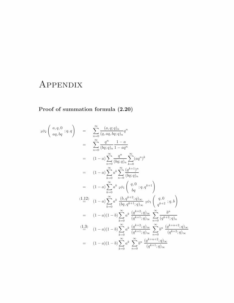
Appendix
Proof of summation formula (2.20)
3!2
"
a, q, 0
aq, bq; q, q
#
=#$
n=0
(a, q; q)n(q, aq, bq; q)n
qn
=#$
n=0
qn
(bq; q)n
1 ! a
1 ! aqn
= (1 ! a)#$
n=0
qn
(bq; q)n
#$
k=0
(aqn)k
= (1 ! a)#$
k=0
ak#$
n=0
(qk+1)n
(bq; q)n
= (1 ! a)#$
k=0
ak2!1
"
q, 0
bq; q, qk+1
#
(1.12)= (1 ! a)
#$
k=0
ak (b, qk+2; q)#(bq, qk+1; q)#
2!1
"
q, 0
qk+2; q, b
#
= (1 ! a)(1 ! b)#$
k=0
ak (qk+2; q)#(qk+1; q)#
#$
n=0
bn
(qk+2; q)n
(1.3)= (1 ! a)(1 ! b)
#$
k=0
ak (qk+2; q)#(qk+1; q)#
#$
n=0
bn (qk+n+2; q)#(qk+2; q)#
= (1 ! a)(1 ! b)#$
k=0
ak#$
n=0
bn (qk+n+2; q)#(qk+1; q)#
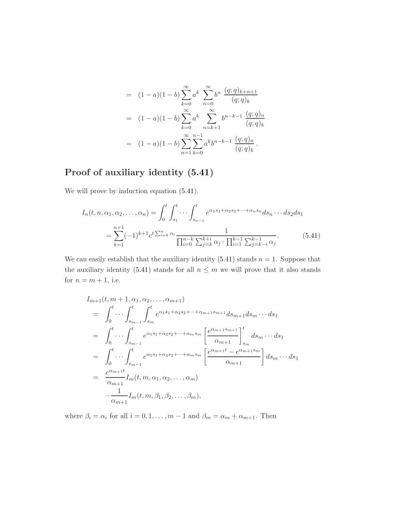
= (1 ! a)(1 ! b)#$
k=0
ak#$
n=0
bn (q; q)k+n+1
(q; q)k
= (1 ! a)(1 ! b)#$
k=0
ak#$
n=k+1
bn$k$1 (q; q)n(q; q)k
= (1 ! a)(1 ! b)#$
n=1
n$1$
k=0
akbn$k$1 (q; q)n(q; q)k
.
Proof of auxiliary identity (5.41)
We will prove by induction equation (5.41).
In(t, n,*1,*2, . . . ,*n) =
+ t
0
+ t
s1
· · ·+ t
sn!1
e+1s1++2s2+···++nsndsn · · · ds2ds1
=n+1$
k=1
(!1)k+1etPn
i=k +i1
6n$ki=0
!k+ij=k *j ·
6k$1i=1
!k$1j=k$i *j
. (5.41)
We can easily establish that the auxiliary identity (5.41) stands n = 1. Suppose that
the auxiliary identity (5.41) stands for all n & m we will prove that it also stands
for n = m + 1, i.e.
Im+1(t,m + 1,*1,*2, . . . ,*m+1)
=
+ t
0· · ·+ t
sm!1
+ t
sm
e+1s1++2s2+···++m+1sm+1dsm+1dsm · · · ds1
=
+ t
0· · ·+ t
sm!1
e+1s1++2s2+···++msm
0
e+m+1sm+1
*m+1
1t
sm
dsm · · · ds1
=
+ t
0· · ·+ t
sm!1
e+1s1++2s2+···++msm
0
e+m+1t ! e+m+1sm
*m+1
1
dsm · · · ds1
=e+m+1t
*m+1Im(t,m,*1,*2, . . . ,*m)
!1
*m+1Im(t,m,-1,-2, . . . ,-m),
where -i = *i for all i = 0, 1, . . . ,m ! 1 and -m = *m + *m+1. Then
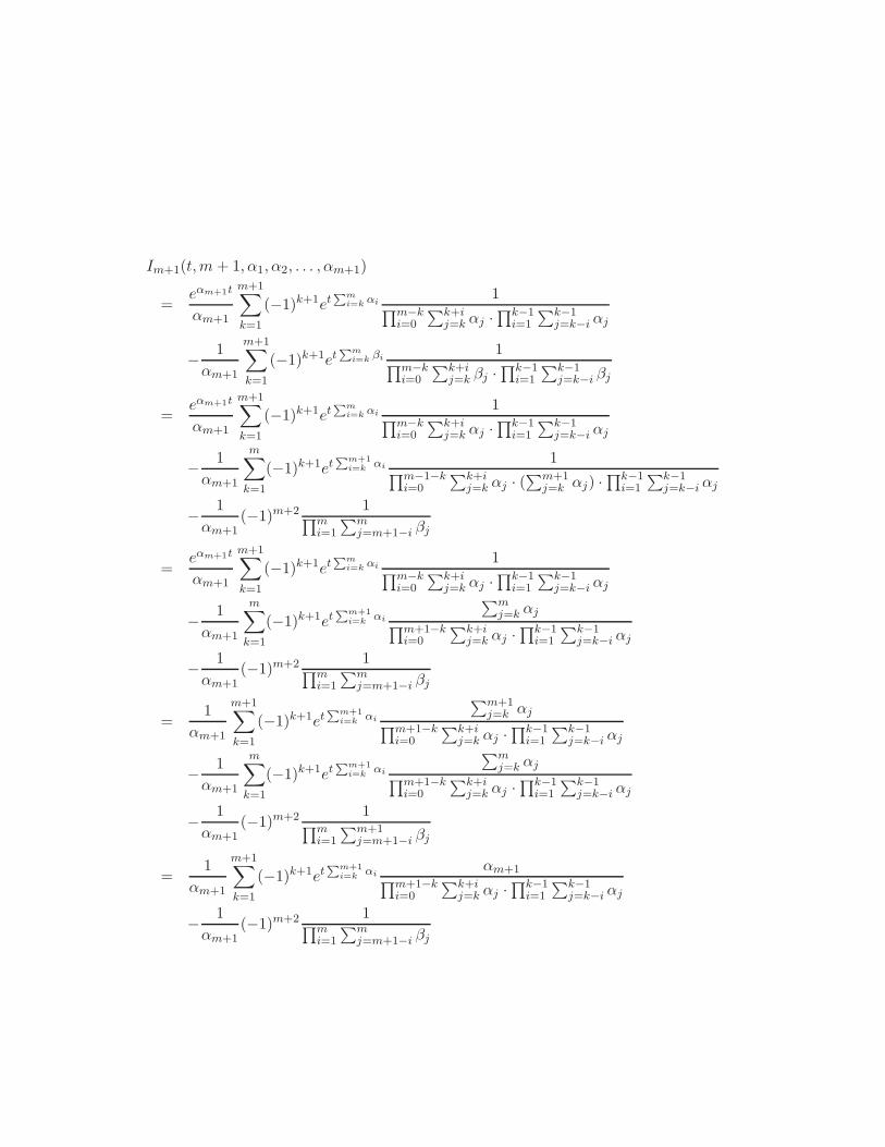
Im+1(t,m + 1,*1,*2, . . . ,*m+1)
=e+m+1t
*m+1
m+1$
k=1
(!1)k+1etPm
i=k +i1
6m$ki=0
!k+ij=k *j ·
6k$1i=1
!k$1j=k$i *j
!1
*m+1
m+1$
k=1
(!1)k+1etPm
i=k ,i1
6m$ki=0
!k+ij=k -j ·
6k$1i=1
!k$1j=k$i -j
=e+m+1t
*m+1
m+1$
k=1
(!1)k+1etPm
i=k +i1
6m$ki=0
!k+ij=k *j ·
6k$1i=1
!k$1j=k$i *j
!1
*m+1
m$
k=1
(!1)k+1etPm+1
i=k +i1
6m$1$ki=0
!k+ij=k *j · (
!m+1j=k *j) ·
6k$1i=1
!k$1j=k$i *j
!1
*m+1(!1)m+2 1
6mi=1
!mj=m+1$i -j
=e+m+1t
*m+1
m+1$
k=1
(!1)k+1etPm
i=k +i1
6m$ki=0
!k+ij=k *j ·
6k$1i=1
!k$1j=k$i *j
!1
*m+1
m$
k=1
(!1)k+1etPm+1
i=k +i
!mj=k *j
6m+1$ki=0
!k+ij=k *j ·
6k$1i=1
!k$1j=k$i *j
!1
*m+1(!1)m+2 1
6mi=1
!mj=m+1$i -j
=1
*m+1
m+1$
k=1
(!1)k+1etPm+1
i=k +i
!m+1j=k *j
6m+1$ki=0
!k+ij=k *j ·
6k$1i=1
!k$1j=k$i *j
!1
*m+1
m$
k=1
(!1)k+1etPm+1
i=k +i
!mj=k *j
6m+1$ki=0
!k+ij=k *j ·
6k$1i=1
!k$1j=k$i *j
!1
*m+1(!1)m+2 1
6mi=1
!m+1j=m+1$i -j
=1
*m+1
m+1$
k=1
(!1)k+1etPm+1
i=k +i*m+1
6m+1$ki=0
!k+ij=k *j ·
6k$1i=1
!k$1j=k$i *j
!1
*m+1(!1)m+2 1
6mi=1
!mj=m+1$i -j
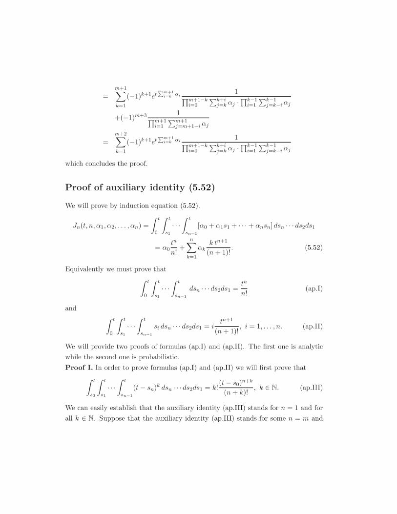
=m+1$
k=1
(!1)k+1etPm+1
i=k +i1
6m+1$ki=0
!k+ij=k *j ·
6k$1i=1
!k$1j=k$i *j
+(!1)m+3 16m+1
i=1
!m+1j=m+1$i *j
=m+2$
k=1
(!1)k+1etPm+1
i=k +i1
6m+1$ki=0
!k+ij=k *j ·
6k$1i=1
!k$1j=k$i *j
which concludes the proof.
Proof of auxiliary identity (5.52)
We will prove by induction equation (5.52).
Jn(t, n,*1,*2, . . . ,*n) =
+ t
0
+ t
s1
· · ·+ t
sn!1
[*0 + *1s1 + · · · + *nsn] dsn · · · ds2ds1
= *0tn
n!+
n$
k=1
*kk tn+1
(n + 1)!. (5.52)
Equivalently we must prove that
+ t
0
+ t
s1
· · ·+ t
sn!1
dsn · · · ds2ds1 =tn
n!(ap.I)
and+ t
0
+ t
s1
· · ·+ t
sn!1
si dsn · · · ds2ds1 = itn+1
(n + 1)!, i = 1, . . . , n. (ap.II)
We will provide two proofs of formulas (ap.I) and (ap.II). The first one is analytic
while the second one is probabilistic.
Proof I. In order to prove formulas (ap.I) and (ap.II) we will first prove that
+ t
s0
+ t
s1
· · ·+ t
sn!1
(t ! sn)k dsn · · · ds2ds1 = k!(t ! s0)n+k
(n + k)!, k % N. (ap.III)
We can easily establish that the auxiliary identity (ap.III) stands for n = 1 and for
all k % N. Suppose that the auxiliary identity (ap.III) stands for some n = m and
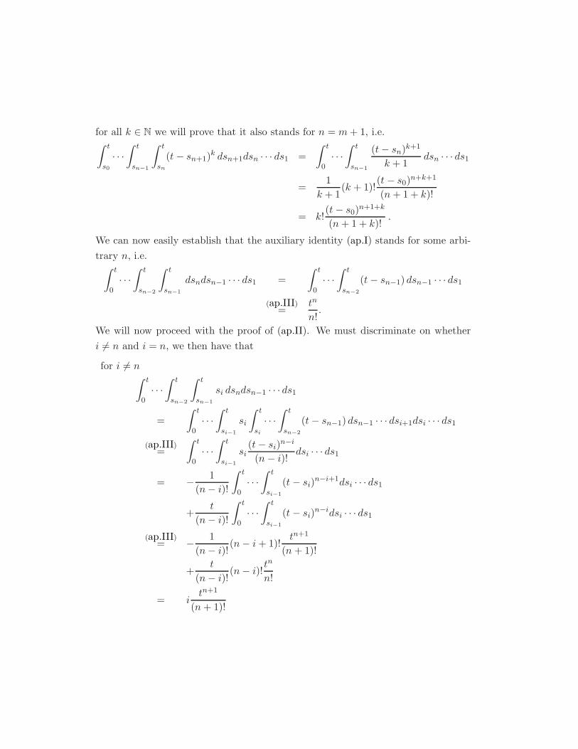
for all k % N we will prove that it also stands for n = m + 1, i.e.+ t
s0
· · ·+ t
sn!1
+ t
sn
(t ! sn+1)k dsn+1dsn · · · ds1 =
+ t
0· · ·+ t
sn!1
(t ! sn)k+1
k + 1dsn · · · ds1
=1
k + 1(k + 1)!
(t ! s0)n+k+1
(n + 1 + k)!
= k!(t ! s0)n+1+k
(n + 1 + k)!.
We can now easily establish that the auxiliary identity (ap.I) stands for some arbi-
trary n, i.e.+ t
0· · ·+ t
sn!2
+ t
sn!1
dsndsn$1 · · · ds1 =
+ t
0· · ·+ t
sn!2
(t ! sn$1) dsn$1 · · · ds1
(ap.III)=
tn
n!.
We will now proceed with the proof of (ap.II). We must discriminate on whether
i (= n and i = n, we then have that
for i (= n+ t
0· · ·+ t
sn!2
+ t
sn!1
si dsndsn$1 · · · ds1
=
+ t
0· · ·+ t
si!1
si
+ t
si
· · ·+ t
sn!2
(t ! sn$1) dsn$1 · · · dsi+1dsi · · · ds1
(ap.III)=
+ t
0· · ·+ t
si!1
si(t ! si)n$i
(n ! i)!dsi · · · ds1
= !1
(n ! i)!
+ t
0· · ·+ t
si!1
(t ! si)n$i+1dsi · · · ds1
+t
(n ! i)!
+ t
0· · ·+ t
si!1
(t ! si)n$idsi · · · ds1
(ap.III)= !
1
(n ! i)!(n ! i + 1)!
tn+1
(n + 1)!
+t
(n ! i)!(n ! i)!
tn
n!
= itn+1
(n + 1)!
for i = n+ t
0· · ·+ t
sn!2
+ t
sn!1
sn dsndsn$1 · · · ds1
= !+ t
0· · ·+ t
sn!2
+ t
sn!1
(t ! sn) dsndsn$1 · · · ds1
+t
+ t
0· · ·+ t
sn!2
+ t
sn!1
dsndsn$1 · · · ds1
(ap.III)= !
tn+1
(n + 1)!+ t
tn
n!
= ntn+1
(n + 1)!.
Proof II. Let U1, U2, . . . , Un be n independent and identical random variables
uniformly distributed over [0, t]. Let U1:n, U2:n, . . . , Un:n be the order statistics of
U1, U2, . . . , Un so that
U1:n & U2:n & . . . & Un:n .
Let f(s1, s2, . . . , sn) be the joint density of U1:n, U2:n, . . . , Un:n. Then it can be shown
that
f(s1, s2, . . . , sn) =
'
(
)
n!tn if 0 & s1 & . . . & sn & t
0 otherwise.(ap.IV)
Then equation (ap.I) can be obtained by
+ t
0
+ t
s1
· · ·+ t
sn!1
f(s1, s2, . . . , sn) dsn · · · ds2ds1 = 1 .
From equation (ap.IV) we derive the marginal density of Ui:n, i = 1, 2, . . . , n, as
fi(u) =n!
(i ! 1)!(n ! i)!
2u
t
3i$1 1
t
2
1 !u
t
3n$i, u % [0, t]. (ap.V)
Then the expected value of Ui:n is given as
E[Ui:n] =it
n + 1. (ap.VI)
To prove equation (ap.II) we rewrite it in the following form
+ t
0
+ t
s1
· · ·+ t
sn!1
sif(s1, s2, . . . , sn) dsn · · · ds2ds1 =it
n + 1, i = 1, . . . , n. (ap.VII)
It is easy to see that the left hand side of equation (ap.VII) is equal to E[Ui:n], which
concludes the proof.

Bibliography
[1] Abate, J., Choudhury, G.L. and Whitt, W. (2000) An introduction to numerical
transform inversion and its application to probability models, in Grassmann,
W.K., ed., Computational Probability, pp.257–323, Kluwer Academic Publish-
ers, Boston.
[2] Adan, I. (1991) A Compensation Approach for Queueing Problems, Doctoral
Thesis, Technische Universiteit Eindhoven, Eindhoven.
[3] Adan, I., Economou, A. and Kapodistria, S. (2009) Synchronized reneging in
queueing systems with vacations, Queueing Systems 62, 1–33.
[4] Adan, I. and van der Wal, J. (1998) Di!erence and Di!erential
Equations in Stochastic Operations Research. Online Notes, URL:
http://www.win.tue.nl/ iadan/
[5] Adan, I. and Weiss, G. (2006) Analysis of a simple Markovian re–entrant line
with infinite supply of work under the LBFS policy. Queueing Systems 54,
169–183.
[6] Ahlfors, L.V. (1979) Complex Analysis, 3rd Edition, McGraw-Hill, Singapore.
[7] Altman, E. and Borovkov, A.A. (1997) On the stability of retrial queues. Queue-
ing Systems 26, 343–363.
[8] Altman, E., and Yechiali, U. (2006) Analysis of customers’ impatience in queues
with server vacations, Queueing Systems 52, 261–279.
[9] Altman, E. and Yechiali, U. (2008) Infinite-server queues with system’s addi-
tional tasks and impatient customers, Probability in the Engineering and Infor-
mational Sciences 22, 477-493.
[10] Altiok, T. (1987) Queues with group arrivals and exhaustive service discipline.
Queueing Systems 2(4), 307-320.
[11] Artalejo, J.R., Economou, A. and Lopez-Herrero, M.J. (2007) Evaluating
growth measures in populations subject to binomial and geometric catastro-
phes, Mathematical Biosciences and Engineering 4, 573–594.
[12] Artalejo, J.R. and Gomez-Corral, A. (1997) Steady state solution of a single-
server queue with linear repeated requests, Journal of Applied Probability 34,
223–233.
[13] Artalejo, J.R. and Pozo, M. (2002) Numerical calculation of the stationary dis-
tribution of the main multiserver retrial queue, Annals of Operations Research
116, 41–56.
[14] Baccelli, F., Boyer, P. and Hebuterne, G. (1984) Single-server queues with
impatient customers. Advances in Applied Probability 16, 887–905.
[15] Baykal-Gursoy M. and Xiao, W. (2004) Stochastic decomposition in M/M/#queues with Markov modulated service rates, Queueing Systems 48, 75–88.
[16] Bini, D.A., Latouche, G. and Meini, B. (2005) Numerical Methods for Structured
Markov Chains, Oxford Science Publications, New York.
[17] Boxma, O.J. and de Waal, P.R. (1994) Multiserver queues with impatient cus-
tomers. ITC 14, 743–756.
[18] Brockwell, P.J., Gani, J. and Resnick, S.I. (1982) Birth, immigration and catas-
trophe processes, Advances in Applied Probability 14, 709–731.
[19] Cohen, J.W. and Boxma, O.J. (1983) Boundary Value Problems in Queueing
System Analysis, North-Holland Mathematics Studies, 79, North-Holland Pub-
lishing Co., Amsterdam.
[20] Cooper, R.B. (1970) Queues served in cyclic order: waiting times. The Bell
System Technical Journal 49, 399-413.
[21] Daley, D.J. (1965) General customer impatience in the queue GI/G/1. Journal
of Applied Probability 2, 186–205.
[22] Denteneer, D., van Leeuwaarden, J.S.H. and Adan, I.J.B.F. (2007) The acqui-
sition queue. Queueing Systems 56(3), 229–240.
[23] Economou, A. (2004) The compound Poisson immigration process subject to
binomial catastrophes, Journal of Applied Probability 41, 508–523.
[24] Economou, A. and Fakinos, D. (2008) Alternative approaches for the transient
analysis of Markov chains with catastrophes, Journal of Statistical Theory and
Practice 2, 183–197.
[25] Economou, A. and Kapodistria, S. (2009) q-series in Markov chains with bi-
nomial transitions: Studying a queue with synchronization, Probability in the
Engineering and Informational Science 23, 75–99.
[26] Economou, A. and Kapodistria, S. (2009) Synchronized abandonments in
a single server unreliable queue, European Journal of Operational Research,
doi:10.1016/j.ejor.2009.07.014.
[27] Fuhrmann, S.W. (1984) A note on the M/G/1 queue with server vacations.
Operations Research 32, 1368–1373.
[28] Gaver, D.P. (1962) A waiting time with interrupted service, including priorities.
Journal of the Royal Statistical Socieity 24, 698-720.
[29] Gail, H.R., Hantler, S.L. and Taylor, B.A. (2000) Use of characteristics roots for
solving infinite state Markov chains, in Grassmann, W.K., ed., Computational
Probability, pp.205–255, Kluwer Academic Publishers, Boston.
[30] Gasper, G. and Rahman, M. (2004) Basic Hypergeometric Series, 2nd Edition,
Cambridge University Press.
[31] Grassmann, W.K. (2002) Real eigenvalues of certain tridiagonal matrix poly-
nomials, with queueing applications, Journal of Linear Algebra and its Appli-
cations 342, 93–106.
[32] Hanschke (1987) Explicit formulas for the characteristics of the M/M/2/2 queue
with repeated attempts. Journal of Applied Probability 24, 486–494.
[33] Harris, C.M. and Marchal, W.G. (1988) State dependence in M/G/1 queue
with generalized vacations. Operations Research, 36(4), 560-565.
[34] Ismail, M.E.H. (1985) A queueing model and a set of orthogonal polynomials,
Journal of Mathematical Analysis and Applications 108, 575–594.
[35] Kao, E.P.C. (1997) An Introduction to Stochastic Processes, Duxbury Press,
Belmont.
[36] Keilson, J. (1962) Queues sub ject to service interruption. Annals Mathematical
Statistics, 33, 1314-1322.
[37] Keilson, J. and Servi, L.D. (1993) The matrix M/M/# system: retrial models
and Markov modulated sources, Advances in Applied Probability 25, 453–471.
[38] Kemp, A.W. and Newton, J. (1990) Certain state-dependent processes for di-
chotomised parasite populations, Journal of Applied Probability 27, 251–258.
[39] Kemp, A.W. (1992) Steady-state Markov chain models for the Heine and Euler
distributions, Journal of Applied Probability 29, 869–876.
[40] Kemp, A.W. (1998) Absorption sampling and absorption distribution, Journal
of Applied Probability 35, 489–494.
[41] Kemp, A.W. (2005) Steady-state Markov chain models for certain q-confluent
hypergeometric distributions, Journal of Statistical Planning and Inference
135, 107–120.
[42] Krantz, S.G. (1999) Handbook of Complex Variables, Birkhanser, Boston.
[43] Krishnamoorthy, A., Deepak, T.G. and Joshua, V.C. (2005) An M/G/1 retrial
queue with nonpersistent customers and orbital search, Stochastic Analysis and
Applications 23, 975–997.
[44] Kroese, D.P., Scheinhardt, W.R.W. and Taylor, P.G. (2004) Spectral properties
of the tandem Jackson network, seen as a quasi-birth-and-death process, Annals
of Applied Probability 14, 2057–2089.
[45] Kulkarni, V.G. (1995) Modeling and Analysis of Stochastic Systems, Chapman
and Hall, London, UK.
[46] Latouche, G. and Ramaswami, V. (1999) Introduction to Matrix-Analytic Meth-
ods in Stochastic Modeling, ASA-SIAM Series on Statistics and Applied Prob-
ability, SIAM, Philadelphia.
[47] Levy, Y. and Yechiali, U. (1975) Utilization for the idle time in an M/G/1
queue with server vacations. Management Science,22, 202-211.
[48] Levy, Y. and Yechiali, U. (1976) An M/M/s queue with server vacations. Cana-
dian Journal of Operational Research and Information Processing, 14, 153-163.
[49] Mitrani, I. and Chakka, R. (1995) Spectral expansion solution for a class
of Markov models: Application and comparison with the matrix-geometric
method, Performance Evaluation 23, 241–260.
[50] Mitrany, I. L. and Avi-Itzhak, B. (1968) A many server queue with service
interruptions. Operational Research, 16(3), 628-638.
[51] Neuts, M.F. (1981) Matrix-geometric Solutions in Stochastic Models: An Algo-
rithmic Approach, Johns Hopkins University Press, Baltimore, MD.
[52] Neuts, M.F. (1989) Structured Stochastic Matrices of M/G/1 Type and Their
Applications, Marcel Dekker Inc., New York.
[53] Neuts, M.F. (1994) An interesting random walk on the nonnegative integers,
Journal of Applied Probability 31, 48–58.
[54] Palm, C. (1953) Methods of judging the annoyance caused by congestion. Tele
4, 189–208.
[55] Palm, C. (1957) Research on telephone tra!c carried by full availability groups.
Tele 1, 107. (English translation of results first published in 1946 in Swedish in
the same journal, which was then entitled Tekniska Meddelanden fran Kungl.
Telegrfstyrelsen).
[56] Perel, N. and Yechiali, U. (2009) Queues with slow servers and impatient cus-
tomers, European Journal of Operational Research.
[57] Ross, S.M. (2003) Introduction to Probability Models (8th ed.), Academic press,
Londen.
[58] Shaked, M. and Shanthikumar, J.G. (1986), Multivariate imperfect repair, Op-
erations Research 34(3), 437-448.
[59] Takacs, L. (1974) A single-server queue with limited virtual waiting time. Jour-
nal of Applied Probability 11, 612–617.
[60] Takagi, H. (1991) Queueing Analysis: A Foundation of Performance Evalu-
ation. Vol. 1. Vacation and Priority Systems, North-Holland Publishing Co.,
Amsterdam.
[61] Tian, N. and Zhang, Z.G. (2006) Vacation Queueing Models. Theory and Ap-
plications, Springer, New York.
[62] Tijms, H.C. (1994) Stochastic Models: An Algorithmic Approach, Wiley, New
York.
[63] Wilf, H. S. (1990) Generatingfunctionology (1st ed.), Academic Press Profes-
sional, Inc., San Diego, CA.
[64] Yadin, M. and Naor, P. (1963) Queueing systems with a removable service
station. Operations Research 14, 393-405.
[65] Yechiali, U. (2007) Queues with system disasters and impatient customers when
system is down, Queueing Systems 56, 195–202.