Stata Press Publication Immediate test of two proportions . . . . . . . . . . . . . . . 53 ... 4.2...

Stata for the Behavioral Sciences

Michael N. Mitchell

®

A Stata Press PublicationSTATA CORPORATIONCollege Station, Texas

® Copyright c© 2015 by StataCorp LPAll rights reserved. First edition 2015

Published by Stata Press, 4905 Lakeway Drive, College Station, Texas 77845Typeset in LATEX2εPrinted in the United States of America

10 9 8 7 6 5 4 3 2 1

ISBN-10: 1-59718-173-0ISBN-13: 978-1-59718-173-0

Library of Congress Control Number: 2015947163

No part of this book may be reproduced, stored in a retrieval system, or transcribed, in anyform or by any means—electronic, mechanical, photocopy, recording, or otherwise—withoutthe prior written permission of StataCorp LP.

Stata, , Stata Press, Mata, , and NetCourse are registered trademarks ofStataCorp LP.

Stata and Stata Press are registered trademarks with the World Intellectual Property Organi-zation of the United Nations.

LATEX2ε is a trademark of the American Mathematical Society.

Contents

Acknowledgments v

List of tables xxiii

List of figures xxv

Preface xxxi

I Warming up 1

1 Introduction 3

1.1 Read me first! . . . . . . . . . . . . . . . . . . . . . . . . . . . . . . . 4

1.1.1 Downloading the example datasets and programs . . . . . . 4

1.1.2 Other user-written programs . . . . . . . . . . . . . . . . . . 4

The fre command . . . . . . . . . . . . . . . . . . . . . . . . 4

The esttab command . . . . . . . . . . . . . . . . . . . . . . 5

The extremes command . . . . . . . . . . . . . . . . . . . . 5

1.2 Why use Stata? . . . . . . . . . . . . . . . . . . . . . . . . . . . . . . 5

1.2.1 ANOVA . . . . . . . . . . . . . . . . . . . . . . . . . . . . . 5

1.2.2 Supercharging your ANOVA . . . . . . . . . . . . . . . . . . 8

1.2.3 Stata is economical . . . . . . . . . . . . . . . . . . . . . . . 8

1.2.4 Statistical powerhouse . . . . . . . . . . . . . . . . . . . . . 8

1.2.5 Easy to learn . . . . . . . . . . . . . . . . . . . . . . . . . . 9

1.2.6 Simple and powerful data management . . . . . . . . . . . . 10

1.2.7 Access to user-written programs . . . . . . . . . . . . . . . . 10

1.2.8 Point and click or commands: Your choice . . . . . . . . . . 11

1.2.9 Powerful yet simple . . . . . . . . . . . . . . . . . . . . . . . 11

1.2.10 Access to Stata source code . . . . . . . . . . . . . . . . . . 11

viii Contents

1.2.11 Online resources for learning Stata . . . . . . . . . . . . . . 11

1.2.12 And yet there is more! . . . . . . . . . . . . . . . . . . . . . 13

1.3 Overview of the book . . . . . . . . . . . . . . . . . . . . . . . . . . . 13

1.3.1 Part I: Warming up . . . . . . . . . . . . . . . . . . . . . . . 13

1.3.2 Part II: Between-subjects ANOVA models . . . . . . . . . . 13

1.3.3 Part III: Repeated measures and longitudinal models . . . . 14

1.3.4 Part IV: Regression models . . . . . . . . . . . . . . . . . . 15

1.3.5 Part V: Stata overview . . . . . . . . . . . . . . . . . . . . . 15

1.3.6 The GSS dataset . . . . . . . . . . . . . . . . . . . . . . . . 16

1.3.7 Language used in the book . . . . . . . . . . . . . . . . . . . 17

1.3.8 Online resources for this book . . . . . . . . . . . . . . . . . 19

1.4 Recommended resources and books . . . . . . . . . . . . . . . . . . . 19

1.4.1 Getting started . . . . . . . . . . . . . . . . . . . . . . . . . 19

1.4.2 Data management in Stata . . . . . . . . . . . . . . . . . . . 20

1.4.3 Reproducing your results . . . . . . . . . . . . . . . . . . . . 20

1.4.4 Recommended Stata Press books . . . . . . . . . . . . . . . 21

2 Descriptive statistics 23

2.1 Chapter overview . . . . . . . . . . . . . . . . . . . . . . . . . . . . . 23

2.2 Using and describing the GSS dataset . . . . . . . . . . . . . . . . . 23

2.3 One-way tabulations . . . . . . . . . . . . . . . . . . . . . . . . . . . 26

2.4 Summary statistics . . . . . . . . . . . . . . . . . . . . . . . . . . . . 31

2.5 Summary statistics by one group . . . . . . . . . . . . . . . . . . . . 32

2.6 Two-way tabulations . . . . . . . . . . . . . . . . . . . . . . . . . . . 34

2.7 Cross-tabulations with summary statistics . . . . . . . . . . . . . . . 37

2.8 Closing thoughts . . . . . . . . . . . . . . . . . . . . . . . . . . . . . 37

3 Basic inferential statistics 39


3.2 Two-sample t tests . . . . . . . . . . . . . . . . . . . . . . . . . . . . 40

3.3 Paired sample t tests . . . . . . . . . . . . . . . . . . . . . . . . . . . 42

3.4 One-sample t tests . . . . . . . . . . . . . . . . . . . . . . . . . . . . 43

Contents ix

3.5 Two-sample test of proportions . . . . . . . . . . . . . . . . . . . . . 43

3.6 One-sample test of proportions . . . . . . . . . . . . . . . . . . . . . 46

3.7 Chi-squared and Fisher’s exact test . . . . . . . . . . . . . . . . . . . 48

3.8 Correlations . . . . . . . . . . . . . . . . . . . . . . . . . . . . . . . . 50

3.9 Immediate commands . . . . . . . . . . . . . . . . . . . . . . . . . . 51

3.9.1 Immediate test of two means . . . . . . . . . . . . . . . . . 51

3.9.2 Immediate test of one mean . . . . . . . . . . . . . . . . . . 52

3.9.3 Immediate test of two proportions . . . . . . . . . . . . . . . 53

3.9.4 Immediate test of one proportion . . . . . . . . . . . . . . . 53

3.9.5 Immediate cross-tabulations . . . . . . . . . . . . . . . . . . 54


II Between-subjects ANOVA models 57

4 One-way between-subjects ANOVA 59


4.2 Comparing two groups using a t test . . . . . . . . . . . . . . . . . . 59

4.3 Comparing two groups using ANOVA . . . . . . . . . . . . . . . . . 63

4.3.1 Computing effect sizes . . . . . . . . . . . . . . . . . . . . . 67

4.4 Comparing three groups using ANOVA . . . . . . . . . . . . . . . . . 69

4.4.1 Testing planned comparisons using contrast . . . . . . . . . 72

4.4.2 Computing effect sizes for planned comparisons . . . . . . . 75

4.5 Estimation commands and postestimation commands . . . . . . . . . 77

4.6 Interpreting confidence intervals . . . . . . . . . . . . . . . . . . . . . 82


5 Contrasts for a one-way ANOVA 85


5.2 Introducing contrasts . . . . . . . . . . . . . . . . . . . . . . . . . . . 86

5.2.1 Computing and graphing means . . . . . . . . . . . . . . . . 88

5.2.2 Making contrasts among means . . . . . . . . . . . . . . . . 89

5.2.3 Graphing contrasts . . . . . . . . . . . . . . . . . . . . . . . 90

x Contents

5.2.4 Options with the margins and contrast commands . . . . . . 92

5.2.5 Computing effect sizes for contrasts . . . . . . . . . . . . . . 96

5.2.6 Summary . . . . . . . . . . . . . . . . . . . . . . . . . . . . 98

5.3 Overview of contrast operators . . . . . . . . . . . . . . . . . . . . . 98

5.4 Compare each group against a reference group . . . . . . . . . . . . . 99

5.4.1 Selecting a specific contrast . . . . . . . . . . . . . . . . . . 100

5.4.2 Selecting a different reference group . . . . . . . . . . . . . . 101

5.4.3 Selecting a contrast and reference group . . . . . . . . . . . 101

5.5 Compare each group against the grand mean . . . . . . . . . . . . . 102


5.6 Compare adjacent means . . . . . . . . . . . . . . . . . . . . . . . . . 105

5.6.1 Reverse adjacent contrasts . . . . . . . . . . . . . . . . . . . 108


5.7 Comparing with the mean of subsequent and previous levels . . . . . 111

5.7.1 Comparing with the mean of previous levels . . . . . . . . . 115


5.8 Polynomial contrasts . . . . . . . . . . . . . . . . . . . . . . . . . . . 117

5.9 Custom contrasts . . . . . . . . . . . . . . . . . . . . . . . . . . . . . 120

5.10 Weighted contrasts . . . . . . . . . . . . . . . . . . . . . . . . . . . . 123

5.11 Pairwise comparisons . . . . . . . . . . . . . . . . . . . . . . . . . . . 125


6 Analysis of covariance 135


6.2 Example 1: ANCOVA with an experiment using a pretest . . . . . . 136

6.3 Example 2: Experiment using covariates . . . . . . . . . . . . . . . . 142

6.4 Example 3: Observational data . . . . . . . . . . . . . . . . . . . . . 146

6.4.1 Model 1: No covariates . . . . . . . . . . . . . . . . . . . . . 147

6.4.2 Model 2: Demographics as covariates . . . . . . . . . . . . . 148

6.4.3 Model 3: Demographics, socializing as covariates . . . . . . 148

6.4.4 Model 4: Demographics, socializing, health as covariates . . 150

Contents xi

6.5 Some technical details about adjusted means . . . . . . . . . . . . . 152

6.5.1 Computing adjusted means: Method 1 . . . . . . . . . . . . 154



6.5.4 Differences between method 2 and method 3 . . . . . . . . . 158

6.5.5 Adjusted means: Summary . . . . . . . . . . . . . . . . . . 160


7 Two-way factorial between-subjects ANOVA 161


7.2 Two-by-two models: Example 1 . . . . . . . . . . . . . . . . . . . . . 163

7.2.1 Simple effects . . . . . . . . . . . . . . . . . . . . . . . . . . 168

7.2.2 Estimating the size of the interaction . . . . . . . . . . . . . 170

7.2.3 More about interaction . . . . . . . . . . . . . . . . . . . . . 171

7.2.4 Summary . . . . . . . . . . . . . . . . . . . . . . . . . . . . 172

7.3 Two-by-three models . . . . . . . . . . . . . . . . . . . . . . . . . . . 173

7.3.1 Example 2 . . . . . . . . . . . . . . . . . . . . . . . . . . . . 173

Simple effects . . . . . . . . . . . . . . . . . . . . . . . . . . 175

Simple contrasts . . . . . . . . . . . . . . . . . . . . . . . . . 176

Partial interaction . . . . . . . . . . . . . . . . . . . . . . . 177

Comparing optimism therapy with traditional therapy . . . 178

7.3.2 Example 3 . . . . . . . . . . . . . . . . . . . . . . . . . . . . 180

Simple effects . . . . . . . . . . . . . . . . . . . . . . . . . . 182

Partial interactions . . . . . . . . . . . . . . . . . . . . . . . 183

7.3.3 Summary . . . . . . . . . . . . . . . . . . . . . . . . . . . . 185

7.4 Three-by-three models: Example 4 . . . . . . . . . . . . . . . . . . . 185

7.4.1 Simple effects . . . . . . . . . . . . . . . . . . . . . . . . . . 188

7.4.2 Simple contrasts . . . . . . . . . . . . . . . . . . . . . . . . . 188

7.4.3 Partial interaction . . . . . . . . . . . . . . . . . . . . . . . 190

7.4.4 Interaction contrasts . . . . . . . . . . . . . . . . . . . . . . 191

7.4.5 Summary . . . . . . . . . . . . . . . . . . . . . . . . . . . . 193

xii Contents

7.5 Unbalanced designs . . . . . . . . . . . . . . . . . . . . . . . . . . . . 193

7.6 Interpreting confidence intervals . . . . . . . . . . . . . . . . . . . . . 198


8 Analysis of covariance with interactions 203


8.2 Example 1: IV has two levels . . . . . . . . . . . . . . . . . . . . . . 206

8.2.1 Question 1: Treatment by depression interaction . . . . . . 210

8.2.2 Question 2: When is optimism therapy superior? . . . . . . 213

8.2.3 Example 1: Summary . . . . . . . . . . . . . . . . . . . . . 219

8.3 Example 2: IV has three levels . . . . . . . . . . . . . . . . . . . . . 220

8.3.1 Questions 1a and 1b . . . . . . . . . . . . . . . . . . . . . . 225

Question 1a . . . . . . . . . . . . . . . . . . . . . . . . . . . 225

Question 1b . . . . . . . . . . . . . . . . . . . . . . . . . . . 226

8.3.2 Questions 2a and 2b . . . . . . . . . . . . . . . . . . . . . . 227

Question 2a . . . . . . . . . . . . . . . . . . . . . . . . . . . 227

Question 2b . . . . . . . . . . . . . . . . . . . . . . . . . . . 228

8.3.3 Overall interaction . . . . . . . . . . . . . . . . . . . . . . . 230

8.3.4 Example 2: Summary . . . . . . . . . . . . . . . . . . . . . 231


9 Three-way between-subjects analysis of variance 233


9.2 Two-by-two-by-two models . . . . . . . . . . . . . . . . . . . . . . . 234

9.2.1 Simple interactions by season . . . . . . . . . . . . . . . . . 236

9.2.2 Simple interactions by depression status . . . . . . . . . . . 237

9.2.3 Simple effects . . . . . . . . . . . . . . . . . . . . . . . . . . 239

9.3 Two-by-two-by-three models . . . . . . . . . . . . . . . . . . . . . . . 240

9.3.1 Simple interactions by depression status . . . . . . . . . . . 242

9.3.2 Simple partial interaction by depression status . . . . . . . . 242

9.3.3 Simple contrasts . . . . . . . . . . . . . . . . . . . . . . . . . 244

9.3.4 Partial interactions . . . . . . . . . . . . . . . . . . . . . . . 244

Contents xiii

9.4 Three-by-three-by-three models and beyond . . . . . . . . . . . . . . 246

9.4.1 Partial interactions and interaction contrasts . . . . . . . . . 248

9.4.2 Simple interactions . . . . . . . . . . . . . . . . . . . . . . . 252

9.4.3 Simple effects and simple contrasts . . . . . . . . . . . . . . 256


10 Supercharge your analysis of variance (via regression) 259


10.2 Performing ANOVA tests via regression . . . . . . . . . . . . . . . . 260

10.3 Supercharging your ANOVA . . . . . . . . . . . . . . . . . . . . . . . 264

10.3.1 Complex surveys . . . . . . . . . . . . . . . . . . . . . . . . 265

10.3.2 Homogeneity of variance . . . . . . . . . . . . . . . . . . . . 269

10.3.3 Robust regression . . . . . . . . . . . . . . . . . . . . . . . . 273

10.3.4 Quantile regression . . . . . . . . . . . . . . . . . . . . . . . 275

10.4 Main effects with interactions: anova versus regress . . . . . . . . . . 276


11 Power analysis for analysis of variance and covariance 281


11.2 Power analysis for a two-sample t test . . . . . . . . . . . . . . . . . 282

11.2.1 Example 1: Replicating a two-group comparison . . . . . . . 282

11.2.2 Example 2: Using standardized effect sizes . . . . . . . . . . 284

11.2.3 Estimating effect sizes . . . . . . . . . . . . . . . . . . . . . 286

11.2.4 Example 3: Power for a medium effect . . . . . . . . . . . . 287

11.2.5 Example 4: Power for a range of effect sizes . . . . . . . . . 288

11.2.6 Example 5: For a given N, compute the effect size . . . . . . 290

11.2.7 Example 6: Compute effect sizes given unequal Ns . . . . . 291

11.3 Power analysis for one-way ANOVA . . . . . . . . . . . . . . . . . . 293

11.3.1 Overview . . . . . . . . . . . . . . . . . . . . . . . . . . . . . 293

Hypothesis 1. Traditional therapy versus control . . . . . . 293

Hypothesis 2: Optimism therapy versus control . . . . . . . 294

xiv Contents

Hypothesis 3: Optimism therapy versus traditional therapy 294

Summary of hypotheses . . . . . . . . . . . . . . . . . . . . 295

11.3.2 Example 7: Testing hypotheses 1 and 2 . . . . . . . . . . . . 295

11.3.3 Example 8: Testing hypotheses 2 and 3 . . . . . . . . . . . . 298

11.3.4 Summary . . . . . . . . . . . . . . . . . . . . . . . . . . . . 301

11.4 Power analysis for ANCOVA . . . . . . . . . . . . . . . . . . . . . . 301

11.4.1 Example 9: Using pretest as a covariate . . . . . . . . . . . 301

11.4.2 Example 10: Using correlated variables as covariates . . . . 303

11.5 Power analysis for two-way ANOVA . . . . . . . . . . . . . . . . . . 306

11.5.1 Example 11: Replicating a two-by-two analysis . . . . . . . 306

11.5.2 Example 12: Standardized simple effects . . . . . . . . . . . 307

11.5.3 Example 13: Standardized interaction effect . . . . . . . . . 309

11.5.4 Summary: Power for two-way ANOVA . . . . . . . . . . . . 309


III Repeated measures and longitudinal designs 311

12 Repeated measures designs 313


12.2 Example 1: One-way within-subjects designs . . . . . . . . . . . . . 314

12.3 Example 2: Mixed design with two groups . . . . . . . . . . . . . . . 319

12.4 Example 3: Mixed design with three groups . . . . . . . . . . . . . . 324

12.5 Comparing models with different residual covariance structures . . . 329

12.6 Example 1 revisited: Using compound symmetry . . . . . . . . . . . 331

12.7 Example 1 revisited again: Using small-sample methods . . . . . . . 333

12.8 An alternative analysis: ANCOVA . . . . . . . . . . . . . . . . . . . 337


13 Longitudinal designs 343


13.2 Example 1: Linear effect of time . . . . . . . . . . . . . . . . . . . . 344

13.3 Example 2: Interacting time with a between-subjects IV . . . . . . . 350

Contents xv

13.4 Example 3: Piecewise modeling of time . . . . . . . . . . . . . . . . . 356

13.5 Example 4: Piecewise effects of time by a categorical predictor . . . 363

13.5.1 Baseline slopes . . . . . . . . . . . . . . . . . . . . . . . . . 367

13.5.2 Treatment slopes . . . . . . . . . . . . . . . . . . . . . . . . 368

13.5.3 Jump at treatment . . . . . . . . . . . . . . . . . . . . . . . 370

13.5.4 Comparisons among groups at particular days . . . . . . . . 372

13.5.5 Summary of example 4 . . . . . . . . . . . . . . . . . . . . . 375


IV Regression models 377

14 Simple and multiple regression 379


14.2 Simple linear regression . . . . . . . . . . . . . . . . . . . . . . . . . 380

14.2.1 Decoding the output . . . . . . . . . . . . . . . . . . . . . . 382

14.2.2 Computing predicted means using the margins command . . 383

14.2.3 Graphing predicted means using the marginsplot command 386

14.3 Multiple regression . . . . . . . . . . . . . . . . . . . . . . . . . . . . 389

14.3.1 Describing the predictors . . . . . . . . . . . . . . . . . . . . 390

14.3.2 Running the multiple regression model . . . . . . . . . . . . 391

14.3.3 Computing adjusted means using the margins command . . 392

14.3.4 Describing the contribution of a predictor . . . . . . . . . . 394

One-unit change . . . . . . . . . . . . . . . . . . . . . . . . . 395

Multiple-unit change . . . . . . . . . . . . . . . . . . . . . . 395

Milestone change in units . . . . . . . . . . . . . . . . . . . 396

One SD change in predictor . . . . . . . . . . . . . . . . . . 397

Partial and semipartial correlation . . . . . . . . . . . . . . 398

14.4 Testing multiple coefficients . . . . . . . . . . . . . . . . . . . . . . . 400

14.4.1 Testing whether coefficients equal zero . . . . . . . . . . . . 400

14.4.2 Testing the equality of coefficients . . . . . . . . . . . . . . . 401

14.4.3 Testing linear combinations of coefficients . . . . . . . . . . 402

xvi Contents


15 More details about the regress command 405


15.2 Regression options . . . . . . . . . . . . . . . . . . . . . . . . . . . . 405

15.3 Redisplaying results . . . . . . . . . . . . . . . . . . . . . . . . . . . 408

15.4 Identifying the estimation sample . . . . . . . . . . . . . . . . . . . . 411

15.5 Stored results . . . . . . . . . . . . . . . . . . . . . . . . . . . . . . . 412

15.6 Storing results . . . . . . . . . . . . . . . . . . . . . . . . . . . . . . . 415

15.7 Displaying results with the estimates table command . . . . . . . . . 417


16 Presenting regression results 419


16.2 Presenting a single model . . . . . . . . . . . . . . . . . . . . . . . . 420

16.3 Presenting multiple models . . . . . . . . . . . . . . . . . . . . . . . 423

16.4 Creating regression tables using esttab . . . . . . . . . . . . . . . . . 427

16.4.1 Presenting a single model with esttab . . . . . . . . . . . . . 428

16.4.2 Presenting multiple models with esttab . . . . . . . . . . . . 435

16.4.3 Exporting results to other file formats . . . . . . . . . . . . 436

16.5 More commands for presenting regression results . . . . . . . . . . . 438

16.5.1 outreg . . . . . . . . . . . . . . . . . . . . . . . . . . . . . . 438

16.5.2 outreg2 . . . . . . . . . . . . . . . . . . . . . . . . . . . . . . 438

16.5.3 xml tab . . . . . . . . . . . . . . . . . . . . . . . . . . . . . 438

16.5.4 coefplot . . . . . . . . . . . . . . . . . . . . . . . . . . . . . 439


17 Tools for model building 443


17.2 Fitting multiple models on the same sample . . . . . . . . . . . . . . 443

17.3 Nested models . . . . . . . . . . . . . . . . . . . . . . . . . . . . . . . 448

17.3.1 Example 1: A simple example . . . . . . . . . . . . . . . . . 449

17.3.2 Example 2: A more realistic example . . . . . . . . . . . . . 451

Contents xvii

17.4 Stepwise models . . . . . . . . . . . . . . . . . . . . . . . . . . . . . . 454


18 Regression diagnostics 457


18.2 Outliers . . . . . . . . . . . . . . . . . . . . . . . . . . . . . . . . . . 458

18.2.1 Standardized residuals . . . . . . . . . . . . . . . . . . . . . 460

18.2.2 Studentized residuals, leverage, Cook’s D . . . . . . . . . . . 463

18.2.3 Graphs of residuals, leverage, and Cook’s D . . . . . . . . . 466

18.2.4 DFBETAs and avplots . . . . . . . . . . . . . . . . . . . . . 467

18.2.5 Running a regression with and without observations . . . . 471

18.3 Nonlinearity . . . . . . . . . . . . . . . . . . . . . . . . . . . . . . . . 472

18.3.1 Checking for nonlinearity graphically . . . . . . . . . . . . . 472

18.3.2 Using scatterplots to check for nonlinearity . . . . . . . . . . 473

18.3.3 Checking for nonlinearity using residuals . . . . . . . . . . . 474

18.3.4 Checking for nonlinearity using a locally weighted smoother 475

18.3.5 Graphing an outcome mean at each level of predictor . . . . 476

18.3.6 Summary . . . . . . . . . . . . . . . . . . . . . . . . . . . . 479

18.3.7 Checking for nonlinearity analytically . . . . . . . . . . . . . 479

Adding power terms . . . . . . . . . . . . . . . . . . . . . . 480

Using factor variables . . . . . . . . . . . . . . . . . . . . . . 481

18.4 Multicollinearity . . . . . . . . . . . . . . . . . . . . . . . . . . . . . 485

18.5 Homoskedasticity . . . . . . . . . . . . . . . . . . . . . . . . . . . . . 487

18.6 Normality of residuals . . . . . . . . . . . . . . . . . . . . . . . . . . 489


19 Power analysis for regression 493


19.2 Power for simple regression . . . . . . . . . . . . . . . . . . . . . . . 493

19.3 Power for multiple regression . . . . . . . . . . . . . . . . . . . . . . 500

19.4 Power for a nested multiple regression . . . . . . . . . . . . . . . . . 500


xviii Contents

V Stata overview 507

20 Common features of estimation commands 509


20.2 Common syntax . . . . . . . . . . . . . . . . . . . . . . . . . . . . . 510

20.3 Analysis using subsamples . . . . . . . . . . . . . . . . . . . . . . . . 511

20.4 Robust standard errors . . . . . . . . . . . . . . . . . . . . . . . . . . 512

20.5 Prefix commands . . . . . . . . . . . . . . . . . . . . . . . . . . . . . 513

20.5.1 The by: prefix . . . . . . . . . . . . . . . . . . . . . . . . . . 513

20.5.2 The nestreg: prefix . . . . . . . . . . . . . . . . . . . . . . . 514

20.5.3 The stepwise: prefix . . . . . . . . . . . . . . . . . . . . . . 515

20.5.4 The svy: prefix . . . . . . . . . . . . . . . . . . . . . . . . . 515

20.5.5 The mi estimate: prefix . . . . . . . . . . . . . . . . . . . . 516

20.6 Setting confidence levels . . . . . . . . . . . . . . . . . . . . . . . . . 516

20.7 Postestimation commands . . . . . . . . . . . . . . . . . . . . . . . . 517


21 Postestimation commands 519


21.2 The contrast command . . . . . . . . . . . . . . . . . . . . . . . . . . 519

21.3 The margins command . . . . . . . . . . . . . . . . . . . . . . . . . . 524

21.3.1 The at() option . . . . . . . . . . . . . . . . . . . . . . . . . 525

21.3.2 Margins with factor variables . . . . . . . . . . . . . . . . . 529

21.3.3 Margins with factor variables and the at() option . . . . . . 533

21.3.4 The dydx() option . . . . . . . . . . . . . . . . . . . . . . . 534

21.4 The marginsplot command . . . . . . . . . . . . . . . . . . . . . . . . 539

21.5 The pwcompare command . . . . . . . . . . . . . . . . . . . . . . . . 550


22 Stata data management commands 557


22.2 Reading data into Stata . . . . . . . . . . . . . . . . . . . . . . . . . 558

22.2.1 Reading Stata datasets . . . . . . . . . . . . . . . . . . . . . 558

Contents xix

22.2.2 Reading Excel workbooks . . . . . . . . . . . . . . . . . . . 559

22.2.3 Reading comma-separated files . . . . . . . . . . . . . . . . 560

22.2.4 Reading other file formats . . . . . . . . . . . . . . . . . . . 560

22.3 Saving data . . . . . . . . . . . . . . . . . . . . . . . . . . . . . . . . 561

22.4 Labeling data . . . . . . . . . . . . . . . . . . . . . . . . . . . . . . . 562

22.4.1 Variable labels . . . . . . . . . . . . . . . . . . . . . . . . . . 563

22.4.2 A looping trick . . . . . . . . . . . . . . . . . . . . . . . . . 563

22.4.3 Value labels . . . . . . . . . . . . . . . . . . . . . . . . . . . 565

22.5 Creating and recoding variables . . . . . . . . . . . . . . . . . . . . . 566

22.5.1 Creating new variables with generate . . . . . . . . . . . . . 566

22.5.2 Modifying existing variables with replace . . . . . . . . . . . 567

22.5.3 Extensions to generate egen . . . . . . . . . . . . . . . . . . 568

22.5.4 Recode . . . . . . . . . . . . . . . . . . . . . . . . . . . . . . 569

22.6 Keeping and dropping variables . . . . . . . . . . . . . . . . . . . . . 570

22.7 Keeping and dropping observations . . . . . . . . . . . . . . . . . . . 572

22.8 Combining datasets . . . . . . . . . . . . . . . . . . . . . . . . . . . . 574

22.8.1 Appending datasets . . . . . . . . . . . . . . . . . . . . . . . 574

22.8.2 Merging datasets . . . . . . . . . . . . . . . . . . . . . . . . 576

22.9 Reshaping datasets . . . . . . . . . . . . . . . . . . . . . . . . . . . . 578

22.9.1 Reshaping datasets wide to long . . . . . . . . . . . . . . . . 578

22.9.2 Reshaping datasets long to wide . . . . . . . . . . . . . . . . 580


23 Stata equivalents of common IBM SPSS Commands 583


23.2 ADD FILES . . . . . . . . . . . . . . . . . . . . . . . . . . . . . . . . 584

23.3 AGGREGATE . . . . . . . . . . . . . . . . . . . . . . . . . . . . . . 586

23.4 ANOVA . . . . . . . . . . . . . . . . . . . . . . . . . . . . . . . . . . 588

23.5 AUTORECODE . . . . . . . . . . . . . . . . . . . . . . . . . . . . . 589

23.6 CASESTOVARS . . . . . . . . . . . . . . . . . . . . . . . . . . . . . 591

23.7 COMPUTE . . . . . . . . . . . . . . . . . . . . . . . . . . . . . . . . 593

xx Contents

23.8 CORRELATIONS . . . . . . . . . . . . . . . . . . . . . . . . . . . . 594

23.9 CROSSTABS . . . . . . . . . . . . . . . . . . . . . . . . . . . . . . . 594

23.10 DATA LIST . . . . . . . . . . . . . . . . . . . . . . . . . . . . . . . . 596

23.11 DELETE VARIABLES . . . . . . . . . . . . . . . . . . . . . . . . . 597

23.12 DESCRIPTIVES . . . . . . . . . . . . . . . . . . . . . . . . . . . . . 599

23.13 DISPLAY . . . . . . . . . . . . . . . . . . . . . . . . . . . . . . . . . 600

23.14 DOCUMENT . . . . . . . . . . . . . . . . . . . . . . . . . . . . . . . 601

23.15 FACTOR . . . . . . . . . . . . . . . . . . . . . . . . . . . . . . . . . 602

23.16 FILTER . . . . . . . . . . . . . . . . . . . . . . . . . . . . . . . . . . 602

23.17 FORMATS . . . . . . . . . . . . . . . . . . . . . . . . . . . . . . . . 603

23.18 FREQUENCIES . . . . . . . . . . . . . . . . . . . . . . . . . . . . . 603

23.19 GET FILE . . . . . . . . . . . . . . . . . . . . . . . . . . . . . . . . 605

23.20 GET TRANSLATE . . . . . . . . . . . . . . . . . . . . . . . . . . . 605

23.21 LOGISTIC REGRESSION . . . . . . . . . . . . . . . . . . . . . . . 606

23.22 MATCH FILES . . . . . . . . . . . . . . . . . . . . . . . . . . . . . . 606

23.23 MEANS . . . . . . . . . . . . . . . . . . . . . . . . . . . . . . . . . . 608

23.24 MISSING VALUES . . . . . . . . . . . . . . . . . . . . . . . . . . . . 608

23.25 MIXED . . . . . . . . . . . . . . . . . . . . . . . . . . . . . . . . . . 610

23.26 MULTIPLE IMPUTATION . . . . . . . . . . . . . . . . . . . . . . . 611

23.27 NOMREG . . . . . . . . . . . . . . . . . . . . . . . . . . . . . . . . . 611

23.28 PLUM . . . . . . . . . . . . . . . . . . . . . . . . . . . . . . . . . . . 612

23.29 PROBIT . . . . . . . . . . . . . . . . . . . . . . . . . . . . . . . . . . 613

23.30 RECODE . . . . . . . . . . . . . . . . . . . . . . . . . . . . . . . . . 614

23.31 RELIABILITY . . . . . . . . . . . . . . . . . . . . . . . . . . . . . . 615

23.32 RENAME VARIABLES . . . . . . . . . . . . . . . . . . . . . . . . . 615

23.33 SAVE . . . . . . . . . . . . . . . . . . . . . . . . . . . . . . . . . . . 617

23.34 SELECT IF . . . . . . . . . . . . . . . . . . . . . . . . . . . . . . . . 618

23.35 SAVE TRANSLATE . . . . . . . . . . . . . . . . . . . . . . . . . . . 618

23.36 SORT CASES . . . . . . . . . . . . . . . . . . . . . . . . . . . . . . . 618

23.37 SORT VARIABLES . . . . . . . . . . . . . . . . . . . . . . . . . . . 619

Contents xxi

23.38 SUMMARIZE . . . . . . . . . . . . . . . . . . . . . . . . . . . . . . . 619

23.39 T-TEST . . . . . . . . . . . . . . . . . . . . . . . . . . . . . . . . . . 619

23.40 VALUE LABELS . . . . . . . . . . . . . . . . . . . . . . . . . . . . . 620

23.41 VARIABLE LABELS . . . . . . . . . . . . . . . . . . . . . . . . . . 621

23.42 VARSTOCASES . . . . . . . . . . . . . . . . . . . . . . . . . . . . . 623


References 625

Author index 627

Subject index 629

Preface

I worked as a statistical consultant at the University of California, Los Angeles, ATS

statistical consulting group for over 12 years. Before the start of every walk-in consultingsession, I would wonder about the questions that would walk into our office. Everysession was different, with people bringing questions from all parts of the campus.When a new client walked in the door, one of my first questions was, What departmentare you from? It might have seemed like a polite question as we got to know each otherbefore diving into the heart of his or her problem. But this was an essential questionfor me: the answer would guide the way I handled the entire visit.

In working as a consultant who served so many schools and departments, I discov-ered that there are many regional dialects of statistics. Depending on your school ordepartment, there are certain types of statistical models you emphasize, customs youembrace, and types of terminology you favor. This is why there are statistics booksthat are written specifically for certain disciplines—to address the statistical customsand traditions within that discipline.

My home discipline is psychology, in which I received my bachelor’s, master’s, anddoctorate. As I was taught statistics, my professors focused on forming specific hypoth-esis tests for the exact predicted pattern of results. They emphasized taking a laserlikefocus on specific contrasts that would directly test the hypothesis of interest. This wasespecially the case when I was taught about factorial analysis of variance (ANOVA),where a finding of an overall interaction effect was nothing to get excited about becausethe significant interaction could be consistent with a variety of patterns of results, someof which could be contrary to our hypotheses. We were taught to graph the interac-tions and probe and dissect the interaction using planned contrasts to test for the exactpattern of results that we hypothesized.

xxxii Preface

I brought this training to my statistical consulting and my use of statistical packages.However, I frequently found that my training regarding ways of dissecting interactionswas not so easily supported by statistical packages—that is, until the most recent ver-sions of Stata. Unlike any other statistical package that I have ever used, Stata providesa suite of tools that allows us to probe, interpret, understand, and graph the resultsof ANOVA models. These tools are incredibly powerful; they are also very simple andintuitive. In this book, I show how you can use this suite of ANOVA tools to easily formcontrasts among groups and dissect interactions with surgical precision. This allows youto present tests of hypotheses regarding the specific pattern of your results, establishingnot only that your results are significant but also that they are in the pattern predicted.The suite of tools also integrates graphing tools so that you can use graphics as a meansof interpreting your results and for presenting results to others.

The heart and spirit of this book is about showcasing this suite of ANOVA tools thatStata offers, but that does not mean this book is limited to just the presentation ofANOVA. This is because this suite of ANOVA tools can be applied to a wide variety of de-signs, including analysis of covariance, analysis of covariance with interactions, repeatedmeasures designs, longitudinal designs, and the analysis of survey data to name just afew. This suite of tools can also be used in the context of a wide variety of regressionmodeling methods, including ordinary regression, robust regression, multilevel models,logistic regression, and Poisson regression.

As I see it, one of the strengths of learning statistics from a behavioral scienceperspective is seeing how factorial designs can help us understand how the effect ofone variable is moderated by another variable through testing of interactions. Withmost statistical packages, you are handcuffed to using these tools only in the contextof a traditional ANOVA. Once you extend your reach outside that realm, these tools aretaken away from you. In Stata, you carry this suite of tools with you as you run amultilevel model, a robust regression, a logistic regression, or even a regression basedon complex survey sampling. In this book, my aim is to show how you can use thesefamiliar tools and to enable you to apply them across a wide variety of designs andmodeling methods.

While this book draws upon my statistical training from the perspective of psychol-ogy, it is written for anyone in the behavioral sciences and anyone who would like tolearn how to apply ANOVA (and ANOVA-like tools) to a variety of designs and modelingtechniques using Stata. Regardless of your home discipline, I hope this book shows howyou can use Stata to understand your results so that you can interpret and present themwith clarity and confidence.

Valencia, California Michael N. MitchellJuly 2015

5 Contrasts for a one-way ANOVA

5.1 Chapter overview . . . . . . . . . . . . . . . . . . . . . . . . . 85

5.2 Introducing contrasts . . . . . . . . . . . . . . . . . . . . . . . 86

5.2.1 Computing and graphing means . . . . . . . . . . . . . . . 88

5.2.2 Making contrasts among means . . . . . . . . . . . . . . . 89

5.2.3 Graphing contrasts . . . . . . . . . . . . . . . . . . . . . . 90

5.2.4 Options with the margins and contrast commands . . . . . 92

5.2.5 Computing effect sizes for contrasts . . . . . . . . . . . . . 96

5.2.6 Summary . . . . . . . . . . . . . . . . . . . . . . . . . . . 98

5.3 Overview of contrast operators . . . . . . . . . . . . . . . . . 98

5.4 Compare each group against a reference group . . . . . . . . . 99

5.4.1 Selecting a specific contrast . . . . . . . . . . . . . . . . . 100

5.4.2 Selecting a different reference group . . . . . . . . . . . . . 101

5.4.3 Selecting a contrast and reference group . . . . . . . . . . 101

5.5 Compare each group against the grand mean . . . . . . . . . 102


5.6 Compare adjacent means . . . . . . . . . . . . . . . . . . . . . 105

5.6.1 Reverse adjacent contrasts . . . . . . . . . . . . . . . . . . 108


5.7 Comparing with the mean of subsequent and previous levels . 111

5.7.1 Comparing with the mean of previous levels . . . . . . . . 115


5.8 Polynomial contrasts . . . . . . . . . . . . . . . . . . . . . . . 117

5.9 Custom contrasts . . . . . . . . . . . . . . . . . . . . . . . . . 120

5.10 Weighted contrasts . . . . . . . . . . . . . . . . . . . . . . . . 123

5.11 Pairwise comparisons . . . . . . . . . . . . . . . . . . . . . . . 125

5.12 Closing thoughts . . . . . . . . . . . . . . . . . . . . . . . . . 133

5.1 Chapter overview

This chapter is devoted to showing you how to perform specific comparisons amonggroups (contrasts) after performing a one-way analysis of variance (ANOVA). Such con-trasts allow you to test for the exact pattern of results that you hypothesized before

85

86 Chapter 5 Contrasts for a one-way ANOVA

the start of your study. This chapter illustrates many different kinds of contrasts thatyou can perform using Stata’s built-in contrast operators. Further, it shows how youcan perform custom contrasts (if you want to perform a contrast that is not among thebuilt-in contrasts).

5.2 Introducing contrasts

It turns out that Professor Cheer is interested in studying happiness as well as studyingoptimism. She is interested in exploring the effect of marital status on happiness. Shedecides to explore this question using the General Social Survey (GSS) dataset from theyear 2012. The use command reads this dataset into memory. (Section 1.1 shows howto download the example datasets.)

. use gss2012_sbs, clear

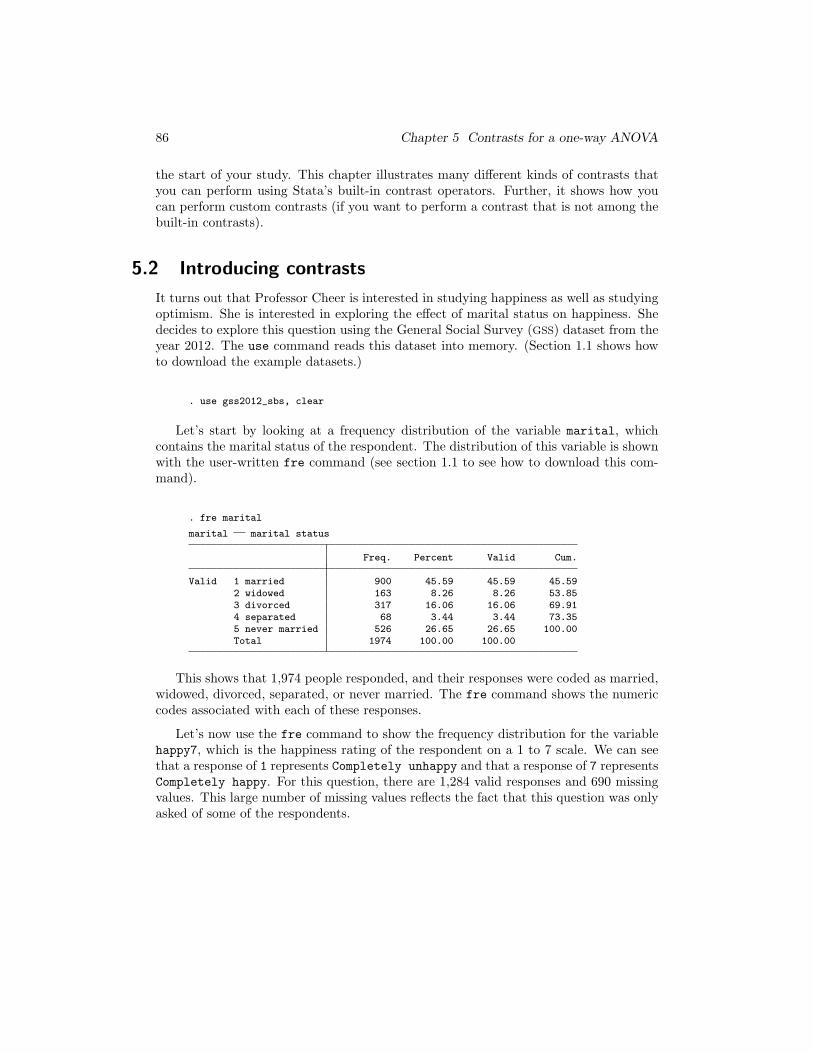
Let’s start by looking at a frequency distribution of the variable marital, whichcontains the marital status of the respondent. The distribution of this variable is shownwith the user-written fre command (see section 1.1 to see how to download this com-mand).

. fre marital

marital marital status

Freq. Percent Valid Cum.

Valid 1 married 900 45.59 45.59 45.592 widowed 163 8.26 8.26 53.853 divorced 317 16.06 16.06 69.914 separated 68 3.44 3.44 73.355 never married 526 26.65 26.65 100.00Total 1974 100.00 100.00

This shows that 1,974 people responded, and their responses were coded as married,widowed, divorced, separated, or never married. The fre command shows the numericcodes associated with each of these responses.

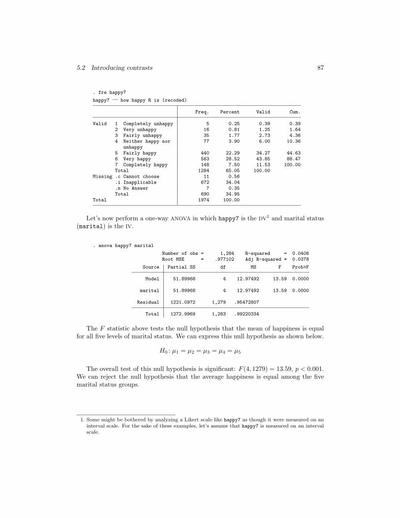
Let’s now use the fre command to show the frequency distribution for the variablehappy7, which is the happiness rating of the respondent on a 1 to 7 scale. We can seethat a response of 1 represents Completely unhappy and that a response of 7 representsCompletely happy. For this question, there are 1,284 valid responses and 690 missingvalues. This large number of missing values reflects the fact that this question was onlyasked of some of the respondents.

5.2 Introducing contrasts 87

. fre happy7

happy7 how happy R is (recoded)

Freq. Percent Valid Cum.

Valid 1 Completely unhappy 5 0.25 0.39 0.392 Very unhappy 16 0.81 1.25 1.643 Fairly unhappy 35 1.77 2.73 4.364 Neither happy nor 77 3.90 6.00 10.36

unhappy5 Fairly happy 440 22.29 34.27 44.636 Very happy 563 28.52 43.85 88.477 Completely happy 148 7.50 11.53 100.00Total 1284 65.05 100.00

Missing .c Cannot choose 11 0.56.i Inapplicable 672 34.04.n No Answer 7 0.35Total 690 34.95

Total 1974 100.00

Let’s now perform a one-way ANOVA in which happy7 is the DV1 and marital status(marital) is the IV.

. anova happy7 marital

Number of obs = 1,284 R-squared = 0.0408Root MSE = .977102 Adj R-squared = 0.0378

Source Partial SS df MS F Prob>F

Model 51.89968 4 12.97492 13.59 0.0000

marital 51.89968 4 12.97492 13.59 0.0000

Residual 1221.0972 1,279 .95472807

Total 1272.9969 1,283 .99220334

The F statistic above tests the null hypothesis that the mean of happiness is equalfor all five levels of marital status. We can express this null hypothesis as shown below.

H0 : µ1 = µ2 = µ3 = µ4 = µ5

The overall test of this null hypothesis is significant: F (4, 1279) = 13.59, p < 0.001.We can reject the null hypothesis that the average happiness is equal among the fivemarital status groups.

1. Some might be bothered by analyzing a Likert scale like happy7 as though it were measured on aninterval scale. For the sake of these examples, let’s assume that happy7 is measured on an intervalscale.


5.2.1 Computing and graphing means

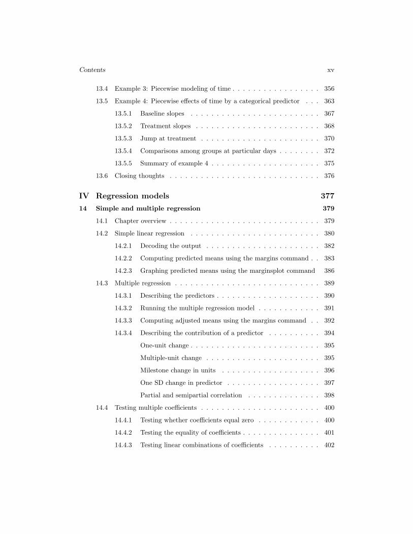
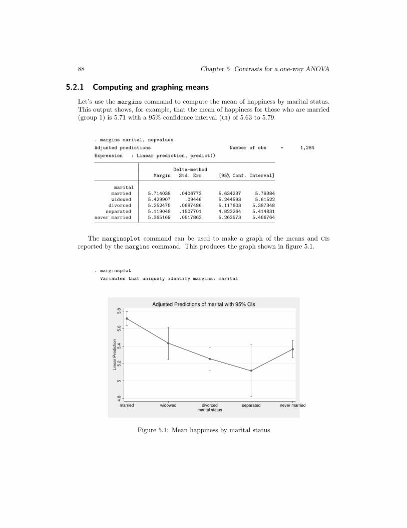
Let’s use the margins command to compute the mean of happiness by marital status.This output shows, for example, that the mean of happiness for those who are married(group 1) is 5.71 with a 95% confidence interval (CI) of 5.63 to 5.79.

. margins marital, nopvalues

Adjusted predictions Number of obs = 1,284

Expression : Linear prediction, predict()

Delta-methodMargin Std. Err. [95% Conf. Interval]

maritalmarried 5.714038 .0406773 5.634237 5.79384widowed 5.429907 .09446 5.244593 5.61522divorced 5.252475 .0687486 5.117603 5.387348

separated 5.119048 .1507701 4.823264 5.414831never married 5.365169 .0517863 5.263573 5.466764

The marginsplot command can be used to make a graph of the means and CIsreported by the margins command. This produces the graph shown in figure 5.1.

. marginsplot

Variables that uniquely identify margins: marital

4.8

55.2

5.4

5.6

5.8

Lin

ear

Pre

dic

tion

married widowed divorced separated never marriedmarital status

Adjusted Predictions of marital with 95% CIs

Figure 5.1: Mean happiness by marital status

5.2.2 Making contrasts among means 89

5.2.2 Making contrasts among means

Let’s probe this finding in more detail. Suppose that Professor Cheer predicted (beforeeven seeing the data) that those who are married will be happier than each of the fourother marital status groups. We can frame this as four separate null hypotheses, shownbelow.

H0#1: µ2 = µ1

H0#2: µ3 = µ1

H0#3: µ4 = µ1

H0#4: µ5 = µ1

The first null hypothesis states that the mean happiness is the same for group 2and group 1 (widowed versus married). The second states that the mean happiness isthe same for groups 3 and 1 (divorced versus married). The third states that the meanhappiness is the same for groups 4 and 1 (separated versus married). Finally, the fourthstates that the mean happiness is the same for groups 5 and 1 (never married versusmarried).

We can test each of these four null hypotheses using the contrast command shownbelow. (I will discuss the syntax of the contrast command shortly.)

. contrast r.marital

Contrasts of marginal linear predictions

Margins : asbalanced

df F P>F

marital(widowed vs married) 1 7.63 0.0058(divorced vs married) 1 33.39 0.0000

(separated vs married) 1 14.52 0.0001(never married vs married) 1 28.07 0.0000

Joint 4 13.59 0.0000

Denominator 1279

Contrast Std. Err. [95% Conf. Interval]

marital(widowed vs married) -.2841316 .1028462 -.4858973 -.0823659(divorced vs married) -.4615629 .0798813 -.6182756 -.3048502

(separated vs married) -.5949905 .156161 -.9013504 -.2886306(never married vs married) -.3488696 .0658518 -.478059 -.2196801

This contrast command compares each marital status group to group 1. The firsttest compares those who are widowed with those who are married. The upper portion of


the output shows the F statistic for the test of this hypothesis. This test is statisticallysignificant: F (1, 1279) = 7.63, p = 0.0058. The lower portion of the output shows thatthe average difference in the happiness for those who are widowed versus married is−0.28, (95% CI = [−0.49,−0.08]). Those who are widowed are significantly less happythan those who are married. Put another way, those who are married are significantlyhappier than those who are widowed. We can reject H0#1 and say the results areconsistent with our prediction that those who are married are significantly happier.

Let’s now consider the output for the second, third, and fourth contrasts. Thesetest the second, third, and fourth null hypotheses contrasting those who are divorcedversus married, separated versus married, and never married versus married. The up-per portion of the contrast output shows that each of these contrasts is statisticallysignificant (ps ≤ 0.001). Further, the differences in the means (as shown in the lowerportion of the output) are always negative, indicating that those who are married arehappier than the group they are compared with. Thus we can reject the second, third,and fourth null hypotheses.

To summarize, we can reject all four null hypotheses. Further, each difference was inthe predicted direction. Those who are married are significantly happier than those whoare widowed, significantly happier than those who are divorced, significantly happierthan those who are separated, and significantly happier than those who have neverbeen married.

5.2.3 Graphing contrasts

Let’s create a graph that visually depicts these contrasts. We first use the margins

command to replicate the results we found above via the contrast command. (Thiswill allow us to then use the marginsplot command to graph the results from themargins command.)

23 Stata equivalents of common IBMSPSS Commands

23.1 Chapter overview . . . . . . . . . . . . . . . . . . . . . . . . . 584

23.2 ADD FILES . . . . . . . . . . . . . . . . . . . . . . . . . . . . 584

23.3 AGGREGATE . . . . . . . . . . . . . . . . . . . . . . . . . . 586

23.4 ANOVA . . . . . . . . . . . . . . . . . . . . . . . . . . . . . . 588

23.5 AUTORECODE . . . . . . . . . . . . . . . . . . . . . . . . . 589

23.6 CASESTOVARS . . . . . . . . . . . . . . . . . . . . . . . . . 591

23.7 COMPUTE . . . . . . . . . . . . . . . . . . . . . . . . . . . . 593

23.8 CORRELATIONS . . . . . . . . . . . . . . . . . . . . . . . . 594

23.9 CROSSTABS . . . . . . . . . . . . . . . . . . . . . . . . . . . 594

23.10 DATA LIST . . . . . . . . . . . . . . . . . . . . . . . . . . . . 596

23.11 DELETE VARIABLES . . . . . . . . . . . . . . . . . . . . . 597

23.12 DESCRIPTIVES . . . . . . . . . . . . . . . . . . . . . . . . . 599

23.13 DISPLAY . . . . . . . . . . . . . . . . . . . . . . . . . . . . . 600

23.14 DOCUMENT . . . . . . . . . . . . . . . . . . . . . . . . . . . 601

23.15 FACTOR . . . . . . . . . . . . . . . . . . . . . . . . . . . . . 602

23.16 FILTER . . . . . . . . . . . . . . . . . . . . . . . . . . . . . . 602

23.17 FORMATS . . . . . . . . . . . . . . . . . . . . . . . . . . . . 603

23.18 FREQUENCIES . . . . . . . . . . . . . . . . . . . . . . . . . 603

23.19 GET FILE . . . . . . . . . . . . . . . . . . . . . . . . . . . . 605

23.20 GET TRANSLATE . . . . . . . . . . . . . . . . . . . . . . . 605

23.21 LOGISTIC REGRESSION . . . . . . . . . . . . . . . . . . . 606

23.22 MATCH FILES . . . . . . . . . . . . . . . . . . . . . . . . . . 606

23.23 MEANS . . . . . . . . . . . . . . . . . . . . . . . . . . . . . . 608

23.24 MISSING VALUES . . . . . . . . . . . . . . . . . . . . . . . . 608

23.25 MIXED . . . . . . . . . . . . . . . . . . . . . . . . . . . . . . 610

23.26 MULTIPLE IMPUTATION . . . . . . . . . . . . . . . . . . . 611

23.27 NOMREG . . . . . . . . . . . . . . . . . . . . . . . . . . . . . 611

23.28 PLUM . . . . . . . . . . . . . . . . . . . . . . . . . . . . . . . 612

23.29 PROBIT . . . . . . . . . . . . . . . . . . . . . . . . . . . . . . 613

23.30 RECODE . . . . . . . . . . . . . . . . . . . . . . . . . . . . . 614

583

584 Chapter 23 Stata equivalents of common IBM SPSS Commands

23.31 RELIABILITY . . . . . . . . . . . . . . . . . . . . . . . . . . 615

23.32 RENAME VARIABLES . . . . . . . . . . . . . . . . . . . . . 615

23.33 SAVE . . . . . . . . . . . . . . . . . . . . . . . . . . . . . . . 617

23.34 SELECT IF . . . . . . . . . . . . . . . . . . . . . . . . . . . . 618

23.35 SAVE TRANSLATE . . . . . . . . . . . . . . . . . . . . . . . 618

23.36 SORT CASES . . . . . . . . . . . . . . . . . . . . . . . . . . . 618

23.37 SORT VARIABLES . . . . . . . . . . . . . . . . . . . . . . . 619

23.38 SUMMARIZE . . . . . . . . . . . . . . . . . . . . . . . . . . . 619

23.39 T-TEST . . . . . . . . . . . . . . . . . . . . . . . . . . . . . . 619

23.40 VALUE LABELS . . . . . . . . . . . . . . . . . . . . . . . . . 620

23.41 VARIABLE LABELS . . . . . . . . . . . . . . . . . . . . . . 621

23.42 VARSTOCASES . . . . . . . . . . . . . . . . . . . . . . . . . 623

23.43 Closing thoughts . . . . . . . . . . . . . . . . . . . . . . . . . 624

23.1 Chapter overview

When taking a language class, you often would have a book that would quickly translateEnglish words into another language (say, Spanish). In some cases, there would beone exact word that was the equivalent of the English word, and in other cases, thetranslation would be a bit more murky. There might be two or more equivalent words,or the words would have similar but not exact meanings. Well, think of this chapteras an IBMR© SPSSR© to Stata translation, where sometimes, the SPSS command has anexact equivalent, and sometimes, there is a little bit more in the translation.

This chapter lists commonly used SPSS commands (in alphabetical order) and showsthe equivalent (or near equivalent) Stata command along with one or more examplesof the Stata command. The aim of this chapter is to help you learn, for example, thatthe Stata equivalent of the SPSS AGGREGATE command is the collapse command andto show a simple example of the collapse command. To that end, the examples areintentionally simple (and sometimes might be overly simplistic). But once you knowthat the command you want is, for example, the collapse command, you can then typehelp collapse and access the Stata documentation for all the details about the use ofthe collapse command.

23.2 ADD FILES

Stata equivalent: appendExample: Consider the file moms.dta, which contains a family ID variable, the mother’sage, race, and whether she graduated from high school.

Stata Press Publication Immediate test of two proportions . . . . . . . . . . . . . . . 53 ... 4.2...

Documents

Transcript of Stata Press Publication Immediate test of two proportions . . . . . . . . . . . . . . . 53 ... 4.2...