Stas$cs’for’Genomics’(140.688)’ - Biostatisticskhansen/teaching/2014/140.668/mt-2014.pdf ·...
25
Sta$s$cs for Genomics (140.688) Instructor: Jeff Leek Slide Credits: Rafael Irizarry, John Storey No announcements today.
Transcript of Stas$cs’for’Genomics’(140.688)’ - Biostatisticskhansen/teaching/2014/140.668/mt-2014.pdf ·...

Sta$s$cs for Genomics (140.688) Instructor: Jeff Leek Slide Credits: Rafael Irizarry, John Storey No announcements today.

PGC-‐1α-‐responsive genes involved in oxida$ve phosphoryla$on are coordinately downregulated in human
diabetes
Mootha et al, Nature Gene$cs July 2003 Data: Affymetrix microarray data on 22,000 genes in skeletal muscle biopsy samples
from 43 males, 17 with normal glucose tolerance (NGT), 8 with impaired glucose tolerance and 18 with Type 2 diabetes (DM2).
In their single gene analysis, a t-‐sta$s$c was calculated for each gene. No significant difference found between NTG and DM2 aXer adjus$ng for mul$ple tes$ng.
Their idea: test 149 a priori defined gene sets for associa$on with disease phenotypes.
Since a second version: Subramanian et al PNAS 2005 Oct 25;102(43):15545-‐50 We prefer: Tian et al PNAS 2005 102 (38): 13544-‐13549 (More later)

Hypothesis testing • Once you have a given score for each gene, how do you
decide on a cut-off?
• p-values are popular.
• But how do we decide on a cut-off?
• Are 0.05 and 0.01 appropriate?
• Are the p-values correct?

Recalculate the Sta$s$c And Compare
Original Sta$s$c

Calcula$ng a P-‐value
{# |Sperm| ≥ |Sobs|} P-‐value = # of Permuta$ons
Observed Sta$s$c = 2

P-‐values
P-value
Frequency
0.0 0.2 0.4 0.6 0.8 1.0
01000
2000
3000
4000
5000
P-value
Frequency
0.0 0.2 0.4 0.6 0.8 1.0
02000400060008000
12000
No Differen$al Expression A Lot of Differen$al Expression

Tip: know what a p-‐value is/isn’t
The probability of observing a sta$s$c that extreme if the null hypothesis is true. The p-‐value is not • Probability the null is true • Probability the alterna$ve is true • A measure of sta$s$cal evidence

an easy mistake to make

a problem

a problem

a problem
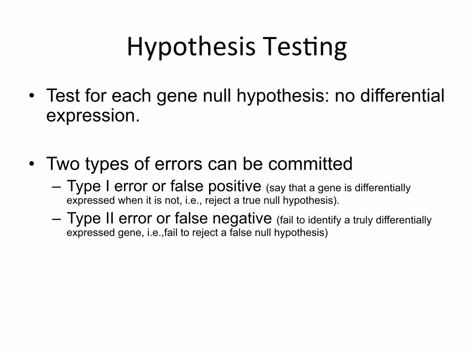
Hypothesis Tes$ng
• Test for each gene null hypothesis: no differential expression.
• Two types of errors can be committed – Type I error or false positive (say that a gene is differentially
expressed when it is not, i.e., reject a true null hypothesis).
– Type II error or false negative (fail to identify a truly differentially expressed gene, i.e.,fail to reject a false null hypothesis)

Hypothe$cal Example
• Microarray with 10,000 genes
• Calculate 10,000 p-‐values
• Call genes “significant” if p-‐value < 0.05
• Expected Number of False Posi$ves:
10,000 × 0.05 = 500 False Posi$ves
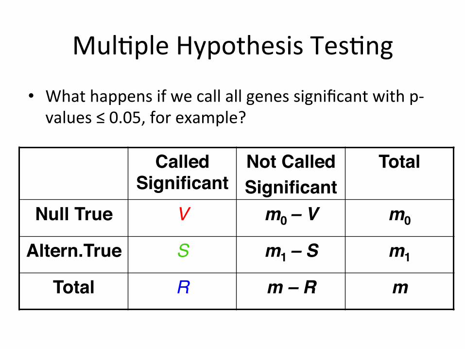
Mul$ple Hypothesis Tes$ng
• What happens if we call all genes significant with p-‐values ≤ 0.05, for example?
Called Significant"
Not Called"Significant"
Total"
Null True" V! m0 – V! m0"
Altern.True" S! m1 – S! m1"
Total" R! m – R! m!
Null = Equivalent Expression; Alternative = Differential Expression

mul$ple comparison error rates • Family wise error rate:
Pr(# False Positives ≥ 1) • False discovery rate:
• EFP (e-‐values) E[# False Positives]
€
E #False Positives# Of Discoveries"
# $ %
& '

False Discovery Rate • The “false discovery rate” measures the propor$on of false
posi$ves among all genes called significant:
• This is usually appropriate because one wants to find as many truly differen$ally expressed genes as possible with rela$vely few false posi$ves
• The false discovery rate gives the rate at which further biological verifica$on will result in dead-‐ends
RV
SVV
=+
=tsignifican called#
positives false#

False Posi$ve Rate versus False Discovery Rate
• False posi$ve rate is the rate at which truly null genes are called significant
• False discovery rate is the rate at which significant genes are truly null
RV
=≈tsignifican called#
positives false#FDR
0nulltruly #positives false#
FPRmV
=≈

Difference in Interpreta$on Suppose 550 out of 10,000 genes are significant at 0.05 level
P-‐value < 0.05 Expect 0.05*10,000 = 500 false posi$ves False Discovery Rate < 0.05 Expect 0.05*550 = 27.5 false posi$ves Family Wise Error Rate < 0.05 The probability of at least 1 false posi$ve ≤ 0.05

Controlling Error Rates
Bonferroni Correc$on (FWER) P-‐values less than α/m are significant
Benjamini-‐Hochberg Correc$on (FDR) Order the p-‐values: p(1) ,…,p(m) If p(i) ≤ α × i/m then it is significant
Correc$ons when doing m tests:

Example With 10 P-‐values
Rank
P-‐value
No Correc$on BH (FDR) Bonferroni (FWER)

False Posi$ve Rate and P-‐values
• The p-‐value is a measure of significance in terms of the false posi$ve rate (aka Type I error rate)
• P-‐value is defined to be the minimum false posi$ve rate at which the sta$s$c can be called significant
• Can be described as the probability a truly null sta$s$c is “as or more extreme” than the observed one

False Discovery Rate and Q-‐values
• The q-‐value is a measure of significance in terms of the false discovery rate
• Q-‐value is defined to be the minimum false discovery rate at which the sta$s$c can be called significant
• Can be described as the probability a sta$s$c “as or more extreme” is truly null

• We begin by es$ma$ng FDR when calling all genes significant with p-‐values ≤ t
• Heuris:c mo$va$on:
[ ][ ]
[ ][ ]} {#E
} {null#E)(E)(E)(FDR
tptp
tRtVt
i
i
≤
≤=≈
Es$mate of FDR
=m0t
} {#ˆ
)(RD̂F 0
tptmt
i ≤
⋅=

Es$mate of π0
• We first es$mate the more easily interpreted π0 = m0/m, the propor$on of truly null (non-‐differen$ally expressed) genes:
• Then clearly
)1(}{#)(ˆ0 λλ
λπ−⋅
>=mpi
mm ⋅= 00 ˆˆ π