Spring 2018 Take-Home Exam 1–Solutions Math 541

1. a. We use information about the Taylor expansions for the exponential and sine functions togive:

f(x) = 2e−2x − 2 cos(2x) + 4 sin(x)

f(x) = 2

(1− 2x+

4x2

2!− 8x3

3!

)− 2

(1− 4x2

2!

)+ 4

(x− x3

3!

)+R3(x)

f(x) = 8x2 − 10

3x3 +R3(x), where P3(x) = 8x2 − 10

3x3.

where

R3(x) =f (4)(ξ(x))x4

4!=

(32e−2ξ(x) − 32 cos(2ξ(x)) + 4 sin(ξ(x)))x4

4!, ξ(x) ∈ [0, x).

b. For x ∈ [0, 1], we have

|R3(x)| ≤ (32 + 32 + 4)

4!=

17

6≈ 2.8333.

(The optimal bound is 0.87556, since f (4)(1) = 21.0133 is largest.) We have f(1) = 4.468848and P3(1) = 14

3 = 4.666667, so the absolute error and relative errors are

|P3(1)− f(1)| = 0.19782

|P3(1)− f(1)||f(1)|

= 0.044266,

where the absolute error is seen to be less than our error bounds computed above.

c. One of the roots of this function is x = 0. The Newton’s method formula is given by

xn+1 = xn −2e−2x − 2 cos(2x) + 4 sin(x)

−4e−2x + 4 sin(2x) + 4 cos(x).

1 function z = newtonth1C(x0,tol,Nmax)2 %NEWTON'S METHOD: Enter f(x), f'(x), x0, tol, Nmax3 f = @(x) 2*exp(-2*x)-2*cos(2*x)+4*sin(x);4 fp = @(x) -4*exp(-2*x)+4*sin(2*x)+4*cos(x);5 xn = x0 - f(x0)/fp(x0);6 z = [x0,xn];7 y = f(xn);8 i = 1;9 fprintf('n = %d, x = %f, f(x) = %f\n', i, xn, y)

10 while (abs(xn - x0) ≥ tol)11 x0 = xn;12 xn = x0 - f(x0)/fp(x0);13 z = [z,xn];14 y = f(xn);15 i = i + 1;16 fprintf('n = %d, x = %f, f(x) = %f\n', i, xn, y)17 if (i ≥ Nmax)18 fprintf('Fail after %d iterations\n',Nmax);

19 break20 end21 end22 end

The Newton iterations are

n xn n xn n xn0 0.3000000 6 0.0040672 12 0.0000634

1 0.1380730 7 0.0020318 13 0.0000317

2 0.0668460 8 0.0010155 14 0.0000159

3 0.0329363 9 0.0005076 15 0.0000079

4 0.0163527 10 0.0002538

5 0.0081482 11 0.0001269

The rate of convergence is linear for the root at x = 0. It takes 15 iterations to converge towithin 10−5. The convergence is only linear because x = 0 is a double root. By examining theCauchy sequence of the iteration,

limn→∞

|xn+1 − xn||xn − xn−1|α

= L,

becomes a line after taking logarithms:

ln (|xn+1 − xn|) = ln(L) + α ln (|xn − xn−1|) .

The linear least squares best fit from the table above gives α = 0.99202 with L = 0.46725.Below is a graph of this convergence:

-12 -10 -8 -6 -4 -2 0ln |xn − xn−1|

-12

-10

-8

-6

-4

-2

ln|x

n+1−xn|

Convergence for Newton (x0 = 0.3)

1 % convergence of Newton's method2 z = newtonth1C(0.3,1e-5,20);3 N = length(z);

4 X = log(abs(z(2:N-1)-z(1:N-2)));5 Y = log(abs(z(3:N)-z(2:N-1)));6 coef = polyfit(X,Y,1)7 yL(1) = coef(1)*X(1)+coef(2);8 yL(2) = coef(1)*X(N-2)+coef(2);9 plot(X,Y,'bo');

10 hold on11 plot([X(1),X(N-2)],[yL(1),yL(2)],'r-');grid;12 title('Convergence for Newton ($x 0 = 0.3$)','FontSize',16,...13 'FontName','Times New Roman','interpreter','latex');14 xlabel('$\ln | x n - x {n-1}|$','FontSize',16,'interpreter','latex');15 ylabel('$\ln | x {n+1} - x n |$','FontSize',16,'interpreter','latex');16 set(gca,'FontSize',14);

d. We use Halley’s method to obtain quadratic convergence to the root at x = 0. This techniqueis given by

xn+1 = xn −f(x)/f ′(x)

[f ′(x)]2 − f(x)f ′′(x),

where f ′(x) = −4 e−2x + 4 sin(2x) + 4 cos(x) and f ′′(x) = 8 e−2x + 8 cos(2x)− 4 sin(x). TheMatLab program for this procedure is:

1 function z = halleyth1C(x0,tol,Nmax)2 %NEWTON'S METHOD: Enter f(x), f'(x), x0, tol, Nmax3 f = @(x) 2*exp(-2*x)-2*cos(2*x)+4*sin(x);4 fp = @(x) -4*exp(-2*x)+4*sin(2*x)+4*cos(x);5 ffp = @(x) 8*exp(-2*x)+8*cos(2*x)-4*sin(x);6 xn = x0 - f(x0).*fp(x0)./(fp(x0).ˆ2-f(x0).*ffp(x0));7 z = [x0,xn];8 y = f(xn);9 i = 1;

10 fprintf('n = %d, x = %f, f(x) = %f\n', i, xn, y)11 while (abs(xn - x0) ≥ tol)12 x0 = xn;13 xn = x0 - f(x0).*fp(x0)./(fp(x0).ˆ2-f(x0).*ffp(x0));14 z = [z,xn];15 y = f(xn);16 i = i + 1;17 fprintf('n = %d, x = %f, f(x) = %f\n', i, xn, y)18 if (i ≥ Nmax)19 fprintf('Fail after %d iterations\n',Nmax);20 break21 end22 end23 end

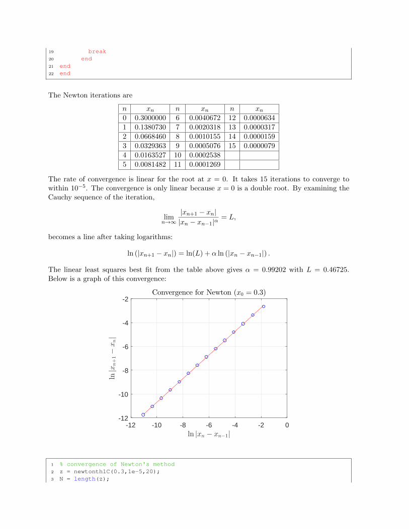
This iteration to a tolerance of 10−8, starting with x0 = 0.3, is given by:

n xn0 0.3

1 2.60295× 10−2

2 1.44384× 10−4

3 4.34370× 10−9

4 3.60007× 10−9

We can see that this method has quadratic convergence because the number of digits ofaccuracy for the solution roughly doubles with each iteration before the 4th iterate. Alternately,if we examine

|xn+1 − x∗||xn − x∗|2

= L,

for the first 3 iterates in the table with x∗ = 0, we obtain L ≈ 0.25, with α = 2, giving quadraticconvergence. Finally, we could use polyfit on these first 3 iterates with the formula:

ln(|xn+1 − x∗|) = α ln(|xn+1 − x∗|) + ln(L),

and obtain α = 2.03689 and L = 0.27712, which agrees with the result above. However, thelast iterate is only a slight improvement. This last iterate suffers from roundoff error in thesubtractions, multiplications, and division. The calculations are too close to the digital limitsof the computer.

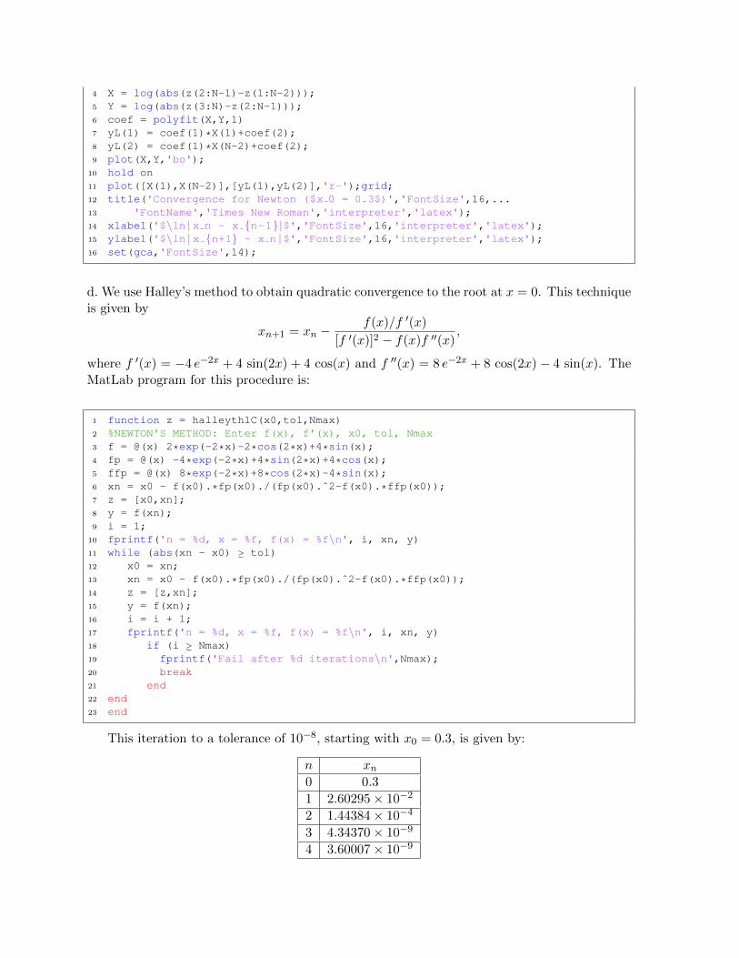
e. There are two other roots of f(x) = 0 for x ∈ (0, 8], which can be seen by the graph of thefunction.

0 2 4 6 8-4

-2

0

2

4

6

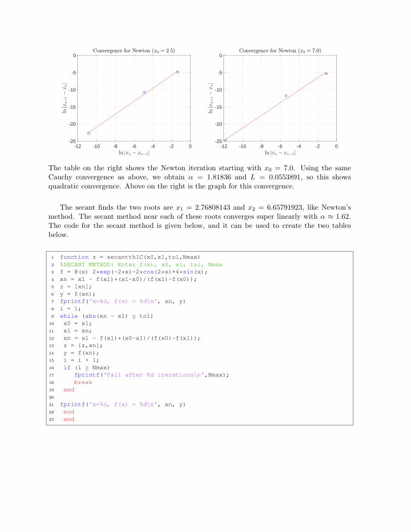
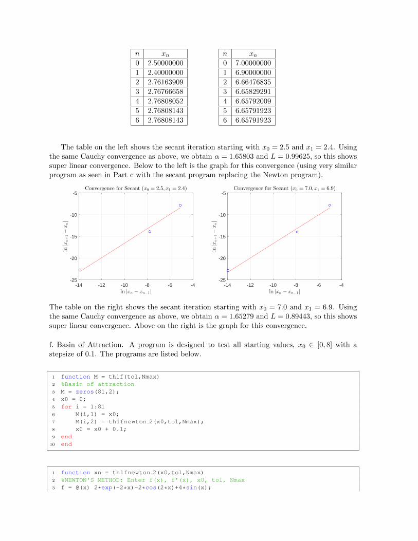
The two other roots are x1 = 2.76808143 and x2 = 6.65791923. The Newton’s method neareach of these roots converges quadratically and is given in the tables below. (This uses thesame program above with different initial conditions.)

n xn0 2.50000000

1 2.76036252

2 2.76806139

3 2.76808143

4 2.76808143

n xn0 7.00000000

1 6.66258788

2 6.65792655

3 6.65791923

4 6.65791923

The table on the left shows the Newton iteration starting with x0 = 2.5. Using the sameCauchy convergence as above, we obtain α = 1.89504 and L = 0.130254, so this shows quadraticconvergence. Below to the left is the graph for this convergence (using very similar program asseen in Part c).

-12 -10 -8 -6 -4 -2 0ln |xn − xn−1|

-25

-20

-15

-10

-5

0

ln|x

n+1−xn|

Convergence for Newton (x0 = 2.5)

-12 -10 -8 -6 -4 -2 0ln |xn − xn−1|

-25

-20

-15

-10

-5

0

ln|x

n+1−xn|

Convergence for Newton (x0 = 7.0)

The table on the right shows the Newton iteration starting with x0 = 7.0. Using the sameCauchy convergence as above, we obtain α = 1.81836 and L = 0.0553891, so this showsquadratic convergence. Above on the right is the graph for this convergence.

The secant finds the two roots are x1 = 2.76808143 and x2 = 6.65791923, like Newton’smethod. The secant method near each of these roots converges super linearly with α ≈ 1.62.The code for the secant method is given below, and it can be used to create the two tablesbelow.

1 function z = secantth1C(x0,x1,tol,Nmax)2 %SECANT METHOD: Enter f(x), x0, x1, tol, Nmax3 f = @(x) 2*exp(-2*x)-2*cos(2*x)+4*sin(x);4 xn = x1 - f(x1)*(x1-x0)/(f(x1)-f(x0));5 z = [xn];6 y = f(xn);7 fprintf('x=%d, f(x) = %d\n', xn, y)8 i = 1;9 while (abs(xn - x1) ≥ tol)

10 x0 = x1;11 x1 = xn;12 xn = x1 - f(x1)*(x0-x1)/(f(x0)-f(x1));13 z = [z,xn];14 y = f(xn);15 i = i + 1;16 if (i ≥ Nmax)17 fprintf('Fail after %d iterations\n',Nmax);18 break19 end20

21 fprintf('x=%d, f(x) = %d\n', xn, y)22 end23 end

n xn0 2.50000000

1 2.40000000

2 2.76163909

3 2.76766658

4 2.76808052

5 2.76808143

6 2.76808143

n xn0 7.00000000

1 6.90000000

2 6.66476835

3 6.65829291

4 6.65792009

5 6.65791923

6 6.65791923

The table on the left shows the secant iteration starting with x0 = 2.5 and x1 = 2.4. Usingthe same Cauchy convergence as above, we obtain α = 1.65803 and L = 0.99625, so this showssuper linear convergence. Below to the left is the graph for this convergence (using very similarprogram as seen in Part c with the secant program replacing the Newton program).

-14 -12 -10 -8 -6 -4ln |xn − xn−1|

-25

-20

-15

-10

-5

ln|x

n+1−xn|

Convergence for Secant (x0 = 2.5, x1 = 2.4)

-14 -12 -10 -8 -6 -4ln |xn − xn−1|

-25

-20

-15

-10

-5

ln|x

n+1−xn|

Convergence for Secant (x0 = 7.0, x1 = 6.9)

The table on the right shows the secant iteration starting with x0 = 7.0 and x1 = 6.9. Usingthe same Cauchy convergence as above, we obtain α = 1.65279 and L = 0.89443, so this showssuper linear convergence. Above on the right is the graph for this convergence.

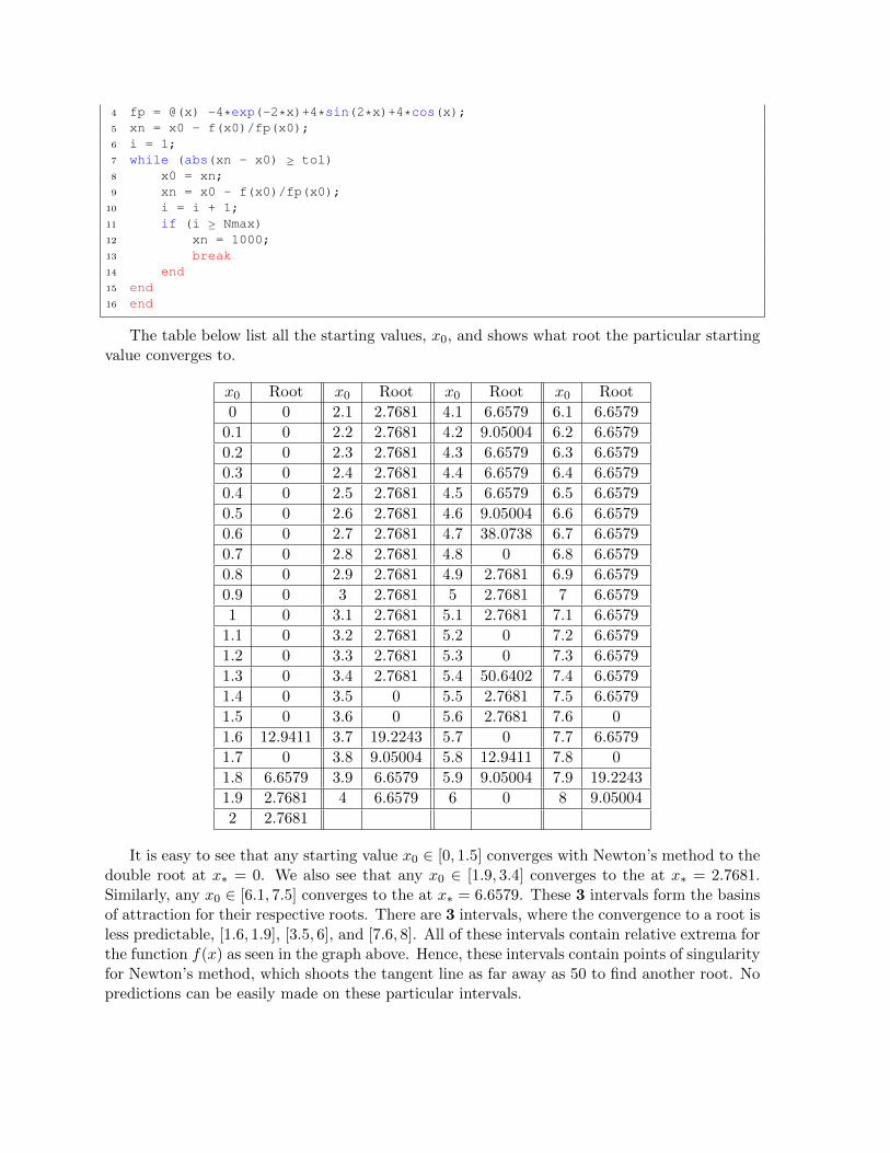
f. Basin of Attraction. A program is designed to test all starting values, x0 ∈ [0, 8] with astepsize of 0.1. The programs are listed below.

1 function M = th1f(tol,Nmax)2 %Basin of attraction3 M = zeros(81,2);4 x0 = 0;5 for i = 1:816 M(i,1) = x0;7 M(i,2) = th1fnewton 2(x0,tol,Nmax);8 x0 = x0 + 0.1;9 end

10 end

1 function xn = th1fnewton 2(x0,tol,Nmax)2 %NEWTON'S METHOD: Enter f(x), f'(x), x0, tol, Nmax3 f = @(x) 2*exp(-2*x)-2*cos(2*x)+4*sin(x);

4 fp = @(x) -4*exp(-2*x)+4*sin(2*x)+4*cos(x);5 xn = x0 - f(x0)/fp(x0);6 i = 1;7 while (abs(xn - x0) ≥ tol)8 x0 = xn;9 xn = x0 - f(x0)/fp(x0);

10 i = i + 1;11 if (i ≥ Nmax)12 xn = 1000;13 break14 end15 end16 end

The table below list all the starting values, x0, and shows what root the particular startingvalue converges to.

x0 Root x0 Root x0 Root x0 Root

0 0 2.1 2.7681 4.1 6.6579 6.1 6.6579

0.1 0 2.2 2.7681 4.2 9.05004 6.2 6.6579

0.2 0 2.3 2.7681 4.3 6.6579 6.3 6.6579

0.3 0 2.4 2.7681 4.4 6.6579 6.4 6.6579

0.4 0 2.5 2.7681 4.5 6.6579 6.5 6.6579

0.5 0 2.6 2.7681 4.6 9.05004 6.6 6.6579

0.6 0 2.7 2.7681 4.7 38.0738 6.7 6.6579

0.7 0 2.8 2.7681 4.8 0 6.8 6.6579

0.8 0 2.9 2.7681 4.9 2.7681 6.9 6.6579

0.9 0 3 2.7681 5 2.7681 7 6.6579

1 0 3.1 2.7681 5.1 2.7681 7.1 6.6579

1.1 0 3.2 2.7681 5.2 0 7.2 6.6579

1.2 0 3.3 2.7681 5.3 0 7.3 6.6579

1.3 0 3.4 2.7681 5.4 50.6402 7.4 6.6579

1.4 0 3.5 0 5.5 2.7681 7.5 6.6579

1.5 0 3.6 0 5.6 2.7681 7.6 0

1.6 12.9411 3.7 19.2243 5.7 0 7.7 6.6579

1.7 0 3.8 9.05004 5.8 12.9411 7.8 0

1.8 6.6579 3.9 6.6579 5.9 9.05004 7.9 19.2243

1.9 2.7681 4 6.6579 6 0 8 9.05004

2 2.7681

It is easy to see that any starting value x0 ∈ [0, 1.5] converges with Newton’s method to thedouble root at x∗ = 0. We also see that any x0 ∈ [1.9, 3.4] converges to the at x∗ = 2.7681.Similarly, any x0 ∈ [6.1, 7.5] converges to the at x∗ = 6.6579. These 3 intervals form the basinsof attraction for their respective roots. There are 3 intervals, where the convergence to a root isless predictable, [1.6, 1.9], [3.5, 6], and [7.6, 8]. All of these intervals contain relative extrema forthe function f(x) as seen in the graph above. Hence, these intervals contain points of singularityfor Newton’s method, which shoots the tangent line as far away as 50 to find another root. Nopredictions can be easily made on these particular intervals.

2. Consider the discrete dynamical model given by

yn = ayn−1 + byn−2, n ≥ 2, a, b ∈ R,

where a, b, y0, y1, and the maximum value of N are inputs. Below is a program that takesthese parameters as input and produces the output y, which can be analyzed. In addition, asemi-log plot is created and is shown below.

1 function y = dynsysC(a,b,y0,y1,N)2 % dynamical system3 y(1) = y0; y(2) = y1;4 for i = 3:N+15 y(i) = a*y(i-1) + b*y(i-2);6 end7 n = 0:N;8 coefa = polyfit(n,log(y),1)9 coef10a = polyfit(n,log10(y),1)

10 Y(1) = exp(coefa(2));11 Y(2) = exp(20*coefa(1)+coefa(2));12 semilogy(n,y,'bo');grid;13 hold on14 semilogy([0,20],[Y(1),Y(2)],'r-');15 title('$y n = y {n-1} + 1.2y {n-2}$','interpreter','latex');16 xlabel('$n$','interpreter','latex');17 ylabel('$y n$','interpreter','latex');18 set(gca,'FontSize',16);19 hold off20

21 print -depsc th3Ca gr.eps22 end

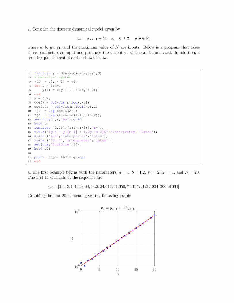
a. The first example begins with the parameters, a = 1, b = 1.2, y0 = 2, y1 = 1, and N = 20.The first 11 elements of the sequence are

yn = [2, 1, 3.4, 4.6, 8.68, 14.2, 24.616, 41.656, 71.1952, 121.1824, 206.61664]

Graphing the first 20 elements gives the following graph:

0 5 10 15 20100

105

If we apply the MatLab program polyfit(n,Y,1), where n = 0:20 and Y = log(y(1:21)),then we obtain the best fitting line is

ln(yn) = 0.52916n+ 0.051689,

log10(yn) = 0.22981n+ 0.022448.

Theoretically, we attempt a solution of the form yn = λn, which when put into the dynamicalmodel gives

λn = aλn−1 + bλn−2 or λn−2(λ2 − aλ− b

)= 0.

Thus, we have a characteristic equation, λ2 − aλ− b = 0. For a = 1 and b = 1.2, we obtainthe real solutions λ1 = −0.70416 and λ2 = 1.70416, which results in the general solution:

yn = c1(−0.70416)n + c2(1.70416)n.

For large n, the first part of this solution is vanishingly small, so asymptotically, yn ≈ c2(1.70416)n,so ln(yn) ≈ ln(c2) + n ln(1.70416). However, ln(1.70416) ≈ .53307, which is fairly close to theslope of the best fitting line above. The graph shows that the best fitting line closely fits thesimulation.From Maple, the actual solution to the difference equation is:

yn = (1.70416)n + (−0.70416)n .

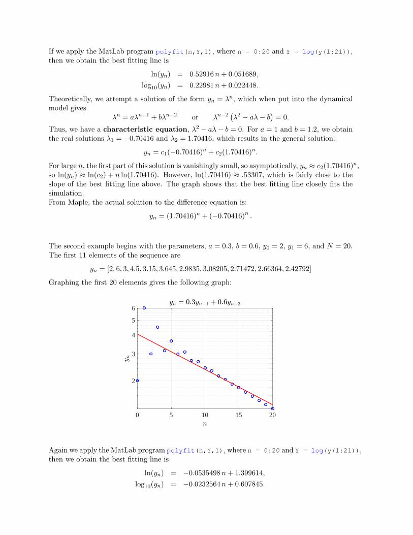
The second example begins with the parameters, a = 0.3, b = 0.6, y0 = 2, y1 = 6, and N = 20.The first 11 elements of the sequence are

yn = [2, 6, 3, 4.5, 3.15, 3.645, 2.9835, 3.08205, 2.71472, 2.66364, 2.42792]

Graphing the first 20 elements gives the following graph:

0 5 10 15 20

2

3

4

5

6

Again we apply the MatLab program polyfit(n,Y,1), where n = 0:20 and Y = log(y(1:21)),then we obtain the best fitting line is

ln(yn) = −0.0535498n+ 1.399614,

log10(yn) = −0.0232564n+ 0.607845.

The characteristic equation for this model is λ2− 0.3λ− 0.6 = 0. It produces the real solutionsλ1 = −0.638987 and λ2 = 0.938987, which results in the general solution:

yn = c1(−0.638987)n + c2(0.938987)n.

For large n, the first part of this solution is vanishingly small, so asymptotically, yn ≈ c2(0.938987)n,so ln(yn) ≈ ln(c2) + n ln(0.934847). However, ln(0.938987) ≈ −0.0629540, which is similar tothe slope of the best fitting line above. The graph shows that the best fitting line moderatelyfits the simulation, but seems to have this slightly more negative slope.From Maple, the actual solution to the difference equation is:

yn = −2.61223 (−0.638987)n + 4.61223 (0.938987)n.

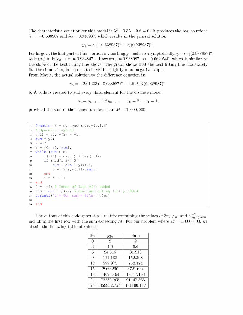
b. A code is created to add every third element for the discrete model:

yn = yn−1 + 1.2 yn−2, y0 = 2, y1 = 1,

provided the sum of the elements is less than M = 1, 000, 000.

1 function Y = dynsysCc(a,b,y0,y1,M)2 % dynamical system3 y(1) = y0; y(2) = y1;4 sum = y0;5 i = 2;6 Y = [0, y0, sum];7 while (sum < M)8 y(i+1) = a*y(i) + b*y(i-1);9 if (mod(i,3)==0)

10 sum = sum + y(i+1);11 Y = [Y;i,y(i+1),sum];12 end13 i = i + 1;14 end15 j = i-4; % Index of last y(i) added16 Sum = sum - y(i); % Sum subtracting last y added17 fprintf('i = %d, sum = %f\n',j,Sum)18

19 end

The output of this code generates a matrix containing the values of 3n, y3n, and∑N

n=0 y3n,including the first row with the sum exceeding M . For our problem where M = 1, 000, 000, weobtain the following table of values:

3n y3n Sum

0 2 2

3 4.6 6.6

6 24.616 31.216

9 121.182 152.398

12 599.975 752.374

15 2969.290 3721.664

18 14695.494 18417.158

21 72730.205 91147.363

24 359952.754 451100.117

Our code requires iterations to y24, and the sum satisfies:

8∑n=0

y3n = 451, 100.117 < 1, 000, 000.

We note that y27 = 1, 781, 460.462, which exceeds M .

3. The Greek mathematician Archimedes estimated the number π by approximating the cir-cumference of a circle of diameter 1 by the perimeter of both inscribed and circumscribedpolygons. The perimeter, tn, of the circumscribed regular polygon with 2n sides can be givenby the recursive formula (tn > π):

tn+1 =

2n+1

(√1 +

(tn2n

)2 − 1

)(tn2n

) , t2 = 4.

a. Below is a MatLab program that satisfies the recursive relation above. It also includes thecorrection needed to produce a modified sequence that maintains accurate calculations.

1 function [T,Z] = circumpi(N)2 %TH question x3 n=2;4 t(2) = 4; z(2) = 4;5 T = zeros(N-1,1); Z = zeros(N-1,1);6 T(1) = t(2); Z(1) = z(2);7 for n=3:N8 t(n) = (2ˆn)*(sqrt(1+(t(n-1)/2ˆ(n-1))ˆ2) - 1)/(t(n-1)/2ˆ(n-1));9 z(n) = 2*z(n-1)/(sqrt(1+(z(n-1)/2ˆ(n-1))ˆ2) + 1);

10 T(n-1) = t(n);11 Z(n-1) = z(n);12 end13 end

The problem in the first sequence is that the quantity in the numerator

limn→∞

√1 +

(tn2n

)2

− 1

= 0,

which has serious subtractive error. This is multiplied by a large number 2n+1 and divided byanother number that tends to zero,

(tn2n

). Thus, we have multiple quantities that cause trouble

in this calculation. The result is the NaN, which appears in the 30th iterate, terminating thesequence.

The program generates the following table:

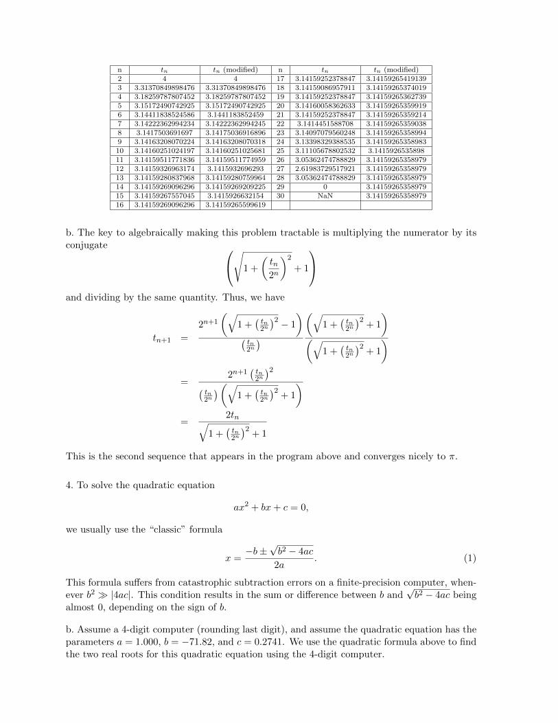
n tn tn (modified) n tn tn (modified)2 4 4 17 3.14159252378847 3.141592654191393 3.31370849898476 3.31370849898476 18 3.14159086957911 3.141592653740194 3.18259787807452 3.18259787807452 19 3.14159252378847 3.141592653627395 3.15172490742925 3.15172490742925 20 3.14160058362633 3.141592653599196 3.14411838524586 3.1441183852459 21 3.14159252378847 3.141592653592147 3.14222362994234 3.14222362994245 22 3.1414451588708 3.141592653590388 3.1417503691697 3.14175036916896 23 3.14097079560248 3.141592653589949 3.14163208070224 3.14163208070318 24 3.13398329388535 3.1415926535898310 3.14160251024197 3.14160251025681 25 3.11105678802532 3.141592653589811 3.14159511771836 3.14159511774959 26 3.05362474788829 3.1415926535897912 3.14159326963174 3.1415932696293 27 2.61983729517921 3.1415926535897913 3.14159280837968 3.14159280759964 28 3.05362474788829 3.1415926535897914 3.14159269096296 3.14159269209225 29 0 3.1415926535897915 3.14159267557045 3.1415926632154 30 NaN 3.1415926535897916 3.14159269096296 3.14159265599619

b. The key to algebraically making this problem tractable is multiplying the numerator by itsconjugate √1 +

(tn2n

)2

+ 1

and dividing by the same quantity. Thus, we have

tn+1 =

2n+1

(√1 +

(tn2n

)2 − 1

)(tn2n

)(√

1 +(tn2n

)2+ 1

)(√

1 +(tn2n

)2+ 1

)=

2n+1(tn2n

)2(tn2n

)(√1 +

(tn2n

)2+ 1

)=

2tn√1 +

(tn2n

)2+ 1

This is the second sequence that appears in the program above and converges nicely to π.

4. To solve the quadratic equation

ax2 + bx+ c = 0,

we usually use the “classic” formula

x =−b±

√b2 − 4ac

2a. (1)

This formula suffers from catastrophic subtraction errors on a finite-precision computer, when-ever b2 � |4ac|. This condition results in the sum or difference between b and

√b2 − 4ac being

almost 0, depending on the sign of b.

b. Assume a 4-digit computer (rounding last digit), and assume the quadratic equation has theparameters a = 1.000, b = −71.82, and c = 0.2741. We use the quadratic formula above to findthe two real roots for this quadratic equation using the 4-digit computer.

We begin by computing b2 = 5158.112, which the computer rounds to 5158. Next wecompute 4ac = 1.0964, which rounds to 1.096. The actual value of b2−4ac = 5157.016, but therounded calculation gives b2 − 4ac = 5157. The actual value of

√b2 − 4ac = 71.81237, while

the rounded value of√b2 − 4ac = 71.81. The next calculations are −b +

√b2 − 4ac, which

gives a precise value of 143.6324 and the rounded value of 143.6. The other calculations are−b−

√b2 − 4ac, which gives a precise value of 0.007633 and the rounded value of 0.01. Dividing

by 2a gives the exact roots r1 = 71.816183 and r2 = 0.003816688. The rounded roots becomeq1 = 71.80 and r2 = 0.005. The percent errors are

100× (q1 − r1)

r1= −0.0225% and 100× (q2 − r2)

r2= 31.0%.

c. As we saw in the previous problem, we can use conjugates to eliminate the square root fromthe numerator. The quadratic formula gives

x =−b±

√b2 − 4ac

2a

=(−b±

√b2 − 4ac)

2a· (−b∓

√b2 − 4ac)

(−b∓√b2 − 4ac)

=4ac

2a(−b∓√b2 − 4ac)

=2c

−b∓√b2 − 4ac

.

Thus, this is an equivalent form of the quadratic formula.Numerically, it is always better to avoid the subtractive error in either the numerator or the

denominator. It follows that we have two cases:

1. If b ≥ 0, then compute the two roots in the following manner:

r1 =−b−

√b2 − 4ac

2aand r2 =

2c

−b−√b2 − 4ac

.

2. If b < 0, then compute the two roots in the following manner:

r1 =2c

−b+√b2 − 4ac

and r2 =−b+

√b2 − 4ac

2a.

Our example in Part b and d provides a good test case.

d. From the alternate formula, we find

q1 =2c

−b−√b2 − 4ac

and q2 =2c

−b+√b2 − 4ac

.

Most of the calculations are similar as performed in Part b. (The exact roots remain thesame with r1 = 71.816183 and r2 = 0.003816688.) With the 4-digit rounding, we still obtain−b−

√b2 − 4ac = 0.01. We compute 2c = 0.5482. Finally, we compute

q1 =2c

−b−√b2 − 4ac

=0.5482

0.01= 54.82.

The percent error with this calculation is

100× (q1 − r1)

r1= −23.67%,

which is significantly worse. With the 4-digit rounding, we still obtain −b+√b2 − 4ac = 143.6.

We compute 2c = 0.5482. Finally, we compute

q2 =2c

−b+√b2 − 4ac

=0.5482

143.6= 0.003818.

The percent error with this calculation is

100× (q2 − r2)

r2= 0.0344%,

which is a significant improvement.

5. a. The functionsf(x) = 1.8 e0.7x and g(x) = 5.3x4.

intersect at 3 points. We begin with graphing the functions to have an estimate of where thefunctions intersect. With normal axes, we divide into two graphs because of the different scalesin y.

-1 -0.5 0 0.5 1x

0

1

2

3

4

5

y

Intersections, Problem 6

f(x)g(x)

0 5 10 15 20x

0

2

4

6

8

y

×105 Intersections, Problem 6

f(x)g(x)

One can see all points of intersection if we use a semilog plot.

-5 0 5 10 15 20x

10-5

100

105

y

Intersections (semilog), Problem 6

f(x)g(x)

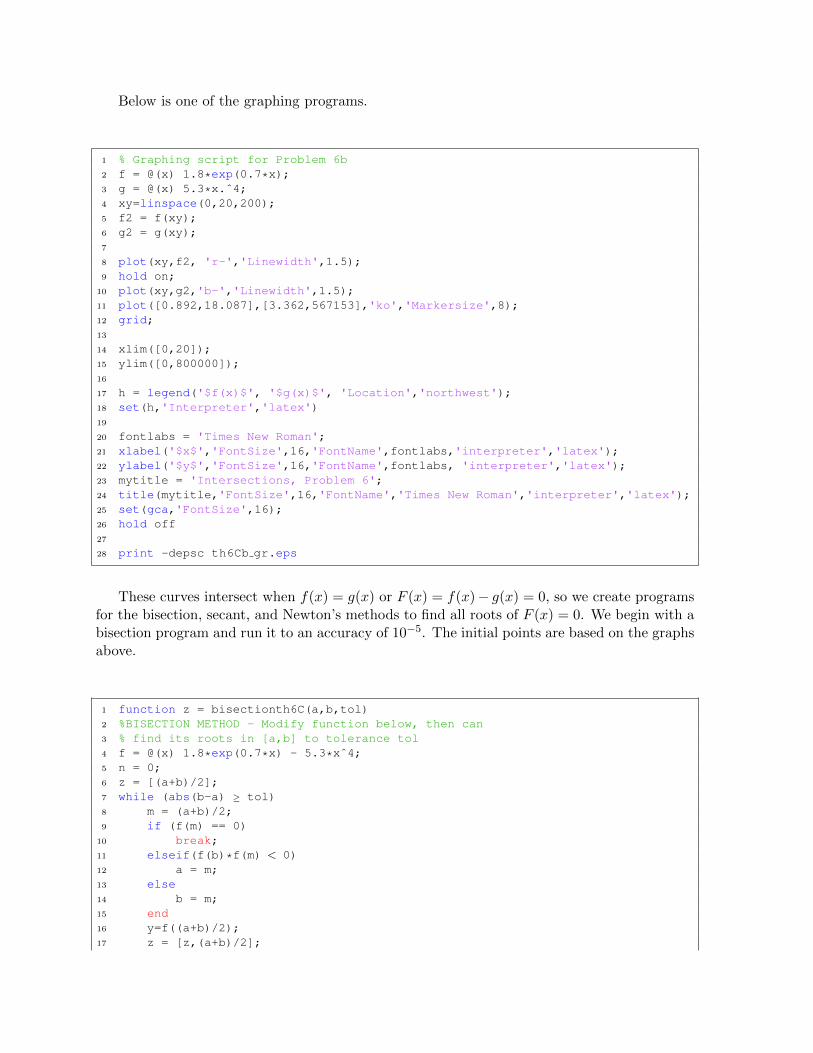
Below is one of the graphing programs.

1 % Graphing script for Problem 6b2 f = @(x) 1.8*exp(0.7*x);3 g = @(x) 5.3*x.ˆ4;4 xy=linspace(0,20,200);5 f2 = f(xy);6 g2 = g(xy);7

8 plot(xy,f2, 'r-','Linewidth',1.5);9 hold on;

10 plot(xy,g2,'b-','Linewidth',1.5);11 plot([0.892,18.087],[3.362,567153],'ko','Markersize',8);12 grid;13

14 xlim([0,20]);15 ylim([0,800000]);16

17 h = legend('$f(x)$', '$g(x)$', 'Location','northwest');18 set(h,'Interpreter','latex')19

20 fontlabs = 'Times New Roman';21 xlabel('$x$','FontSize',16,'FontName',fontlabs,'interpreter','latex');22 ylabel('$y$','FontSize',16,'FontName',fontlabs, 'interpreter','latex');23 mytitle = 'Intersections, Problem 6';24 title(mytitle,'FontSize',16,'FontName','Times New Roman','interpreter','latex');25 set(gca,'FontSize',16);26 hold off27

28 print -depsc th6Cb gr.eps

These curves intersect when f(x) = g(x) or F (x) = f(x)− g(x) = 0, so we create programsfor the bisection, secant, and Newton’s methods to find all roots of F (x) = 0. We begin with abisection program and run it to an accuracy of 10−5. The initial points are based on the graphsabove.

1 function z = bisectionth6C(a,b,tol)2 %BISECTION METHOD - Modify function below, then can3 % find its roots in [a,b] to tolerance tol4 f = @(x) 1.8*exp(0.7*x) - 5.3*xˆ4;5 n = 0;6 z = [(a+b)/2];7 while (abs(b-a) ≥ tol)8 m = (a+b)/2;9 if (f(m) == 0)

10 break;11 elseif(f(b)*f(m) < 0)12 a = m;13 else14 b = m;15 end16 y=f((a+b)/2);17 z = [z,(a+b)/2];

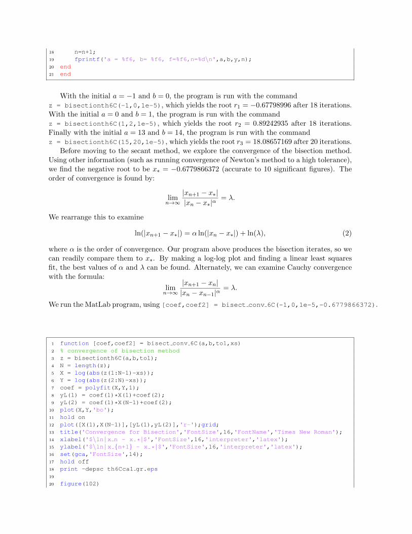
18 n=n+1;19 fprintf('a = %f6, b= %f6, f=%f6,n=%d\n',a,b,y,n);20 end21 end

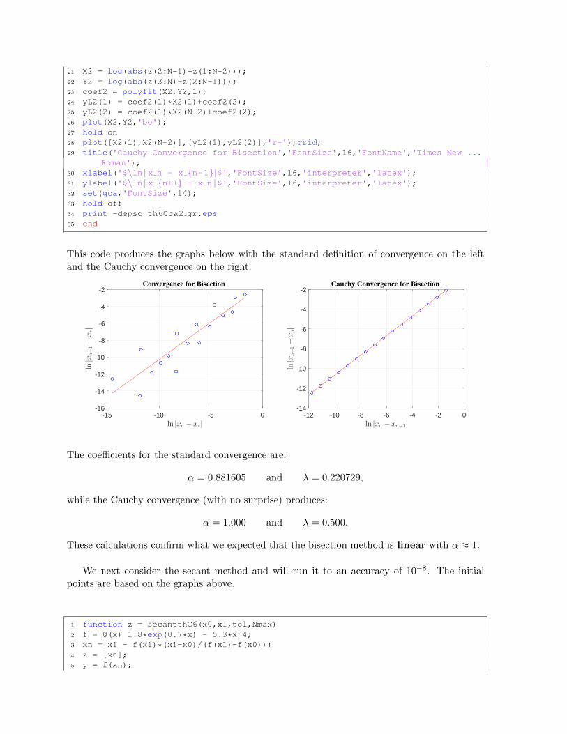
With the initial a = −1 and b = 0, the program is run with the commandz = bisectionth6C(-1,0,1e-5), which yields the root r1 = −0.67798996 after 18 iterations.With the initial a = 0 and b = 1, the program is run with the commandz = bisectionth6C(1,2,1e-5), which yields the root r2 = 0.89242935 after 18 iterations.Finally with the initial a = 13 and b = 14, the program is run with the commandz = bisectionth6C(15,20,1e-5), which yields the root r3 = 18.08657169 after 20 iterations.

Before moving to the secant method, we explore the convergence of the bisection method.Using other information (such as running convergence of Newton’s method to a high tolerance),we find the negative root to be x∗ = −0.6779866372 (accurate to 10 significant figures). Theorder of convergence is found by:

limn→∞

|xn+1 − x∗||xn − x∗|α

= λ.

We rearrange this to examine

ln(|xn+1 − x∗|) = α ln(|xn − x∗|) + ln(λ), (2)

where α is the order of convergence. Our program above produces the bisection iterates, so wecan readily compare them to x∗. By making a log-log plot and finding a linear least squaresfit, the best values of α and λ can be found. Alternately, we can examine Cauchy convergencewith the formula:

limn→∞

|xn+1 − xn||xn − xn−1|α

= λ.

We run the MatLab program, using [coef,coef2] = bisect conv 6C(-1,0,1e-5,-0.6779866372).

1 function [coef,coef2] = bisect conv 6C(a,b,tol,xs)2 % convergence of bisection method3 z = bisectionth6C(a,b,tol);4 N = length(z);5 X = log(abs(z(1:N-1)-xs));6 Y = log(abs(z(2:N)-xs));7 coef = polyfit(X,Y,1);8 yL(1) = coef(1)*X(1)+coef(2);9 yL(2) = coef(1)*X(N-1)+coef(2);

10 plot(X,Y,'bo');11 hold on12 plot([X(1),X(N-1)],[yL(1),yL(2)],'r-');grid;13 title('Convergence for Bisection','FontSize',16,'FontName','Times New Roman');14 xlabel('$\ln | x n - x * |$','FontSize',16,'interpreter','latex');15 ylabel('$\ln | x {n+1} - x * |$','FontSize',16,'interpreter','latex');16 set(gca,'FontSize',14);17 hold off18 print -depsc th6Cca1 gr.eps19

20 figure(102)

21 X2 = log(abs(z(2:N-1)-z(1:N-2)));22 Y2 = log(abs(z(3:N)-z(2:N-1)));23 coef2 = polyfit(X2,Y2,1);24 yL2(1) = coef2(1)*X2(1)+coef2(2);25 yL2(2) = coef2(1)*X2(N-2)+coef2(2);26 plot(X2,Y2,'bo');27 hold on28 plot([X2(1),X2(N-2)],[yL2(1),yL2(2)],'r-');grid;29 title('Cauchy Convergence for Bisection','FontSize',16,'FontName','Times New ...

Roman');30 xlabel('$\ln | x n - x {n-1}|$','FontSize',16,'interpreter','latex');31 ylabel('$\ln | x {n+1} - x n |$','FontSize',16,'interpreter','latex');32 set(gca,'FontSize',14);33 hold off34 print -depsc th6Cca2 gr.eps35 end

This code produces the graphs below with the standard definition of convergence on the leftand the Cauchy convergence on the right.

-15 -10 -5 0ln |xn − x∗|

-16

-14

-12

-10

-8

-6

-4

-2

ln|x

n+1−x∗|

Convergence for Bisection

-12 -10 -8 -6 -4 -2 0ln |xn − xn−1|

-14

-12

-10

-8

-6

-4

-2ln|x

n+1−xn|

Cauchy Convergence for Bisection

The coefficients for the standard convergence are:

α = 0.881605 and λ = 0.220729,

while the Cauchy convergence (with no surprise) produces:

α = 1.000 and λ = 0.500.

These calculations confirm what we expected that the bisection method is linear with α ≈ 1.

We next consider the secant method and will run it to an accuracy of 10−8. The initialpoints are based on the graphs above.

1 function z = secantthC6(x0,x1,tol,Nmax)2 f = @(x) 1.8*exp(0.7*x) - 5.3*xˆ4;3 xn = x1 - f(x1)*(x1-x0)/(f(x1)-f(x0));4 z = [xn];5 y = f(xn);

6 fprintf('x=%d, f(x) = %d\n', xn, y)7 i = 1;8 while (abs(xn - x1) ≥ tol)9 x0 = x1;

10 x1 = xn;11 xn = x1 - f(x1)*(x0-x1)/(f(x0)-f(x1));12 z = [z,xn];13 y = f(xn);14 i = i + 1;15 if (i ≥ Nmax)16 fprintf('Fail after %d iterations\n',Nmax);17 break18 end19

20 fprintf('x=%d, f(x) = %d\n', xn, y)21 end22 end

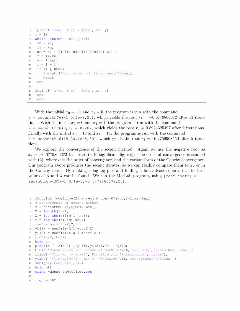
With the initial x0 = −1 and x1 = 0, the program is run with the commandz = secantthC6(-1,0,1e-8,20), which yields the root r1 = −0.6779866372 after 13 itera-tions. With the initial x0 = 0 and x1 = 1, the program is run with the commandz = secantthC6(0,1,1e-8,20), which yields the root r2 = 0.8924325497 after 9 iterations.Finally with the initial x0 = 13 and x1 = 14, the program is run with the commandz = secantthC6(15,20,1e-8,30), which yields the root r3 = 16.2759908550 after 5 itera-tions.

We explore the convergence of the secant method. Again we use the negative root asx∗ = −0.6779866372 (accurate to 10 significant figures). The order of convergence is studiedwith (2), where α is the order of convergence, and the variant form of the Cauchy convergence.Our program above produces the secant iterates, so we can readily compare them to x∗ or inthe Cauchy sense. By making a log-log plot and finding a linear least squares fit, the bestvalues of α and λ can be found. We run the MatLab program, using [coef,coef2] = ...

secant conv 6C(-1,0,1e-8,-0.6779866372,20).

1 function [coef,coef2] = secant conv 6C(a,b,tol,xs,Nmax)2 % convergence of secant method3 z = secantthC6(a,b,tol,Nmax);4 N = length(z)-1;5 X = log(abs(z(1:N-1)-xs));6 Y = log(abs(z(2:N)-xs));7 coef = polyfit(X,Y,1);8 yL(1) = coef(1)*X(1)+coef(2);9 yL(2) = coef(1)*X(N-1)+coef(2);

10 plot(X,Y,'bo');11 hold on12 plot([X(1),X(N-1)],[yL(1),yL(2)],'r-');grid;13 title('Convergence for Secant','FontSize',16,'FontName','Times New Roman');14 xlabel('$\ln | x n - x * |$','FontSize',16,'interpreter','latex');15 ylabel('$\ln | x {n+1} - x * |$','FontSize',16,'interpreter','latex');16 set(gca,'FontSize',14);17 hold off18 print -depsc th6Ccb1 gr.eps19

20 figure(102)

21 X2 = log(abs(z(2:N-1)-z(1:N-2)));22 Y2 = log(abs(z(3:N)-z(2:N-1)));23 coef2 = polyfit(X2,Y2,1);24 yL2(1) = coef2(1)*X2(1)+coef2(2);25 yL2(2) = coef2(1)*X2(N-2)+coef2(2);26 plot(X2,Y2,'bo');27 hold on28 plot([X2(1),X2(N-2)],[yL2(1),yL2(2)],'r-');grid;29 title('Cauchy Convergence for Secant','FontSize',16,'FontName','Times New ...

Roman');30 xlabel('$\ln | x n - x {n-1}|$','FontSize',16,'interpreter','latex');31 ylabel('$\ln | x {n+1} - x n |$','FontSize',16,'interpreter','latex');32 set(gca,'FontSize',14);33 hold off34 print -depsc th6Ccb2 gr.eps35 end

This code produces the graphs below with the standard definition of convergence on the leftand the Cauchy convergence on the right.

-20 -15 -10 -5 0ln |xn − x∗|

-25

-20

-15

-10

-5

0

ln|x

n+1−x∗|

Convergence for Secant

-15 -10 -5 0 5ln |xn − xn−1|

-20

-15

-10

-5

0

5ln|x

n+1−xn|

Cauchy Convergence for Secant

The coefficients for the standard convergence are:

α = 1.523647 and λ = 1.190484,

while the Cauchy convergence produces:

α = 1.470615 and λ = 0.828452.

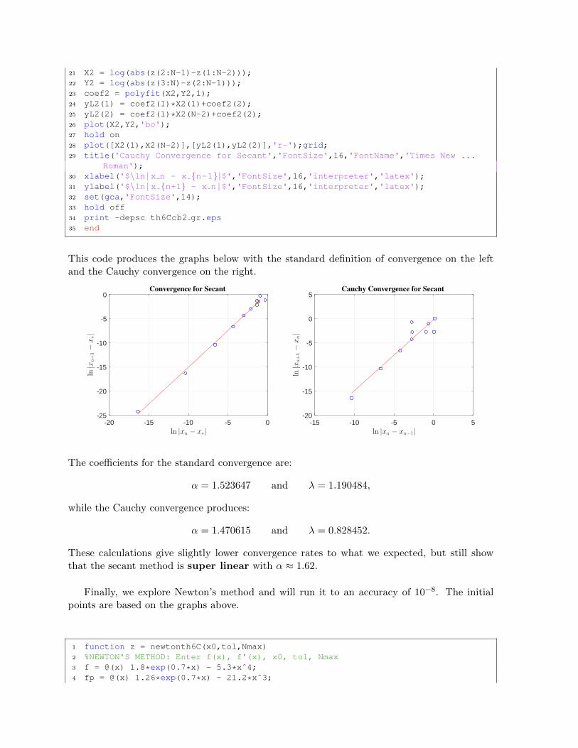
These calculations give slightly lower convergence rates to what we expected, but still showthat the secant method is super linear with α ≈ 1.62.

Finally, we explore Newton’s method and will run it to an accuracy of 10−8. The initialpoints are based on the graphs above.

1 function z = newtonth6C(x0,tol,Nmax)2 %NEWTON'S METHOD: Enter f(x), f'(x), x0, tol, Nmax3 f = @(x) 1.8*exp(0.7*x) - 5.3*xˆ4;4 fp = @(x) 1.26*exp(0.7*x) - 21.2*xˆ3;

5 xn = x0 - f(x0)/fp(x0);6 z = [x0,xn];7 y = f(xn);8 i = 1;9 fprintf('n = %d, x = %f, f(x) = %f\n', i, xn, y)

10 while (abs(xn - x0) ≥ tol)11 x0 = xn;12 xn = x0 - f(x0)/fp(x0);13 z = [z,xn];14 y = f(xn);15 i = i + 1;16 fprintf('n = %d, x = %f, f(x) = %f\n', i, xn, y)17 if (i ≥ Nmax)18 fprintf('Fail after %d iterations\n',Nmax);19 break20 end21 end22 end

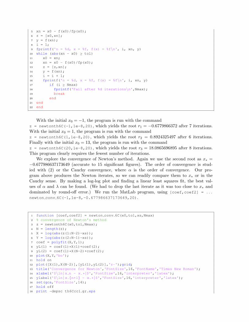
With the initial x0 = −1, the program is run with the commandz = newtonth6C(-1,1e-8,20), which yields the root r1 = −0.6779866372 after 7 iterations.With the initial x0 = 1, the program is run with the commandz = newtonth6C(1,1e-8,20), which yields the root r2 = 0.8924325497 after 6 iterations.Finally with the initial x0 = 13, the program is run with the commandz = newtonth6C(20,1e-8,20), which yields the root r3 = 18.0865696895 after 8 iterations.This program clearly requires the fewest number of iterations.

We explore the convergence of Newton’s method. Again we use the second root as x∗ =−0.677986637173649 (accurate to 15 significant figures). The order of convergence is stud-ied with (2) or the Cauchy convergence, where α is the order of convergence. Our pro-gram above produces the Newton iterates, so we can readily compare them to x∗ or in theCauchy sense. By making a log-log plot and finding a linear least squares fit, the best val-ues of α and λ can be found. (We had to drop the last iterate as it was too close to x∗ anddominated by round-off error.) We run the MatLab program, using [coef,coef2] = ...

newton conv 6C(-1,1e-8,-0.677986637173649,20).

1 function [coef,coef2] = newton conv 6C(x0,tol,xs,Nmax)2 % convergence of Newton's method3 z = newtonth6C(x0,tol,Nmax);4 N = length(z);5 X = log(abs(z(1:N-2)-xs));6 Y = log(abs(z(2:N-1)-xs));7 coef = polyfit(X,Y,1);8 yL(1) = coef(1)*X(1)+coef(2);9 yL(2) = coef(1)*X(N-2)+coef(2);

10 plot(X,Y,'bo');11 hold on12 plot([X(1),X(N-2)],[yL(1),yL(2)],'r-');grid;13 title('Convergence for Newton','FontSize',16,'FontName','Times New Roman');14 xlabel('$\ln | x n - x * |$','FontSize',16,'interpreter','latex');15 ylabel('$\ln | x {n+1} - x * |$','FontSize',16,'interpreter','latex');16 set(gca,'FontSize',14);17 hold off18 print -depsc th6Ccc1 gr.eps

19

20 figure(102)21 X2 = log(abs(z(2:N-1)-z(1:N-2)));22 Y2 = log(abs(z(3:N)-z(2:N-1)));23 coef2 = polyfit(X2,Y2,1);24 yL2(1) = coef2(1)*X2(1)+coef2(2);25 yL2(2) = coef2(1)*X2(N-2)+coef2(2);26 plot(X2,Y2,'bo');27 hold on28 plot([X2(1),X2(N-2)],[yL2(1),yL2(2)],'r-');grid;29 title('Cauchy Convergence for Newton','FontSize',16,'FontName','Times New ...

Roman');30 xlabel('$\ln | x n - x {n-1}|$','FontSize',16,'interpreter','latex');31 ylabel('$\ln | x {n+1} - x n |$','FontSize',16,'interpreter','latex');32 set(gca,'FontSize',14);33 hold off34 print -depsc th6Ccc2 gr.eps35 end

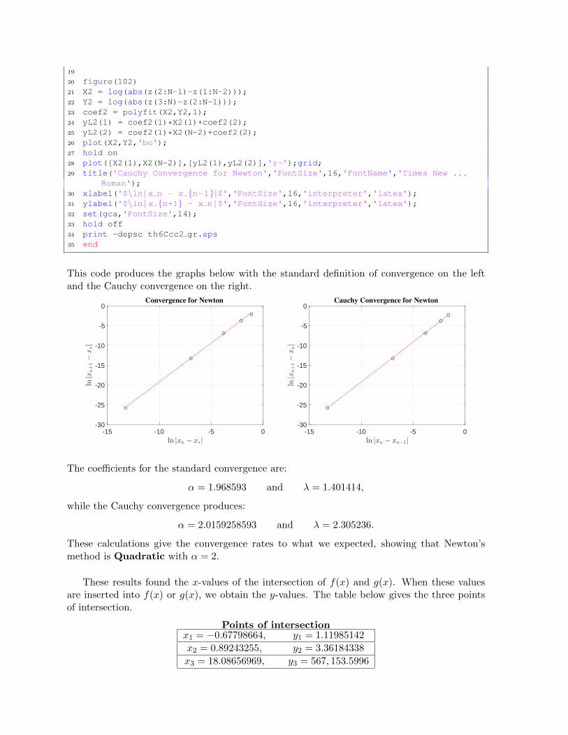
This code produces the graphs below with the standard definition of convergence on the leftand the Cauchy convergence on the right.

-15 -10 -5 0ln |xn − x∗|

-30

-25

-20

-15

-10

-5

0

ln|x

n+1−x∗|

Convergence for Newton

-15 -10 -5 0ln |xn − xn−1|

-30

-25

-20

-15

-10

-5

0

ln|x

n+1−xn|

Cauchy Convergence for Newton

The coefficients for the standard convergence are:

α = 1.968593 and λ = 1.401414,

while the Cauchy convergence produces:

α = 2.0159258593 and λ = 2.305236.

These calculations give the convergence rates to what we expected, showing that Newton’smethod is Quadratic with α = 2.

These results found the x-values of the intersection of f(x) and g(x). When these valuesare inserted into f(x) or g(x), we obtain the y-values. The table below gives the three pointsof intersection.

Points of intersectionx1 = −0.67798664, y1 = 1.11985142

x2 = 0.89243255, y2 = 3.36184338

x3 = 18.08656969, y3 = 567, 153.5996