SplayNet: Towards Locally Self-Adjusting NetworksStefan Schmid∗, Chen Avin∗, Christian Scheideler, Michael Borokhovich, Bernhard Haeupler, Zvi Lotker

Abstract—This paper initiates the study of locally self-adjusting networks: networks whose topology adapts dynamicallyand in a decentralized manner, to the communication pattern σ.Our vision can be seen as a distributed generalization of the self-adjusting datastructures introduced by Sleator and Tarjan [22]:In contrast to their splay trees which dynamically optimize thelookup costs from a single node (namely the tree root), we seekto minimize the routing cost between arbitrary communicationpairs in the network.

As a first step, we study distributed binary search trees(BSTs), which are attractive for their support of greedy routing.We introduce a simple model which captures the fundamentaltradeoff between the benefits and costs of self-adjusting networks.We present the SplayNet algorithm and formally analyze itsperformance, and prove its optimality in specific case studies. Wealso introduce lower bound techniques based on interval cuts andedge expansion, to study the limitations of any demand-optimizednetwork. Finally, we extend our study to multi-tree networks, andhighlight an intriguing difference between classic and distributedsplay trees.

I. INTRODUCTION

In the 1980s, Sleator and Tarjan [22] proposed an appealingnew paradigm to design efficient Binary Search Tree (BST)datastructures: rather than optimizing traditional metrics suchas the search tree depth in the worst-case, their splay datastruc-ture self-adjusts to its usage pattern, moving more frequentlyaccessed elements closer to the root. A natural performancemetric to evaluate a self-adjusting system is the amortized cost:the “average cost” for a worst case sequence of operations (ofa certain class).

Since this seminal work, self-adjusting datastructures havebeen studied intensively, and various more efficient self-adjusting datastructures such as Tango BSTs [7] or multi-splay trees [23] have been proposed. In particular, the fa-mous Dynamic Optimality conjecture [7] continues to puzzleresearchers: the conjecture claims that splay trees perform aswell as any other binary search tree algorithm up to a constantfactor.

In contrast to these flexible classic datastructures, today’sdistributed datastructures and networks are still optimized

S. Schmid is with the TU Berlin & Telekom Innovation Laboratories,Germany, e-mail: stefan@net.t-labs.tu-berlin.de

C. Avin and Z. Lotker are with the Department of Communica-tion Systems Engineering, Ben-Gurion University of the Negev, e-mail:avin,zvilo@bgu.ac.il.

C. Scheideler is with the University of Paderborn, Germany, e-mail:scheideler@upb.de

M. Borokhovich is with the University of Texas at Austin, USA, e-mail:michaelbor@gmail.com

B. Haeupler is with the School of Computer Science, Carnegie MellonUniversity, e-mail: haeupler@cs.cmu.edu.

Conference versions of this work were published in [3], [5].Research supported by the German Israeli G.I.F. Research Grant I-1245-

407.6/2014.∗ The first two authors contributed equally to this work.

toward static metrics, such as the diameter or the length ofthe longest route: the self-adjusting paradigm has not spilledover to distributed networks yet.

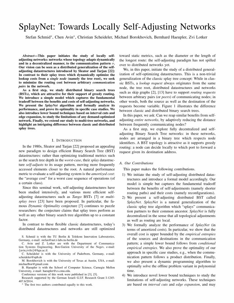
We, in this paper, initiate the study of a distributed general-ization of self-optimizing datastructures. This is a non-trivialgeneralization of the classic splay tree concept: While in clas-sic BSTs, a lookup request always originates from the samenode, the tree root, distributed datastructures and networkssuch as skip graphs [2], [13] have to support routing requestsbetween arbitrary pairs (or peers) of communicating nodes; inother words, both the source as well as the destination of therequests become variable. Figure 1 illustrates the differencebetween classic and distributed binary search trees.

In this paper, we ask: Can we reap similar benefits from self-adjusting entire networks, by adaptively reducing the distancebetween frequently communicating nodes?

As a first step, we explore fully decentralized and self-adjusting Binary Search Tree networks: in these networks,nodes are arranged in a binary tree which respects nodeidentifiers. A BST topology is attractive as it supports greedyrouting: a node can decide locally to which port to forward arequest given its destination address.

A. Our Contributions

This paper makes the following contributions.1) We initiate the study of self-adjusting distributed datas-

tructures and introduce a formal model accordingly. Ourmodel is simple but captures the fundamental tradeoffbetween the benefits of self-adjustments (namely shorterrouting paths) and their costs (namely reconfigurations).

2) We present a self-adjusting distributed BST calledSplayNet. SplayNet is a natural generalization of theclassic splay tree algorithm which “splays” communica-tion partners to their common ancestor. SplayNet is fullydecentralized in the sense that all topological adjustmentsas well as routing are local.

3) We formally analyze the performance of SplayNet (interms of amortized costs). In particular, we show that theoverall cost is upper bounded by the empirical entropiesof the sources and destinations in the communicationpattern; a simple lower bound follows from conditionalempirical entropies. We also prove the optimality of ourapproach in specific case studies, e.g., when the commu-nication pattern follows a product distribution. Finally,we also present a dynamic programming algorithm tooptimally solve the offline problem variant in polynomialtime.

4) We introduce novel lower bound techniques to study thelimitations of self-adjusting networks. These techniquesare based on interval cuts and edge expansion, and may

2

be of independent interest and find applications beyondthe setting studied in this paper.

5) Finally, we initiate the discussion of more complexself-adjusting networks, namely topologies consistingof multiple trees. We make the interesting observationthat in contrast to classic datastructures where the self-adjustment benefits of multiple trees is limited, in adistributed setting, a single additional BST can sometimesreduce the amortized cost dramatically.

In summary, our work shows that while some algorithmicconcepts of traditional splay trees can be generalized tonetworks, the distributed setting requires new analytical tools.Moreover, our results highlight that self-adjustment benefitscan indeed be reaped also in the context of networks; formulti-tree networks, these benefits can even be significantlyhigher than in classic datastructures.

In general, we regard our study as a first step, and believethat our model and results open a rich area for future research.

B. Paper Organization

The upcoming Section II introduces our formal modeland provides the reader with the necessary background. Sec-tion III describes an offline algorithm to compute optimalstatic distributed BSTs and presents the SplayNet approach.Section IV derives entropy-based upper and lower boundson the performance of SplayNets, and Section V studies thelocality and convergence properties of the SplayNet algorithmin specific scenarios. Section VI then derives improved lowerbounds which allow us to show the optimality of SplayNets inadditional scenarios. In Section VII we initiate the discussionof datastructures based on multiple BSTs. After reviewingrelated work in Section VIII, we conclude our contribution inSection IX. In the Appendix, some additional technical detailsare provided.

II. MODEL AND BACKGROUND

We consider a set of n nodes (or peers) V = 1, . . . , ninteracting according to a certain communication pattern. Thepattern is modeled by σ = (σ0, σ1 . . . σm−1): a sequence ofm communication requests where σt = (u, v) ∈ V × V , withsource u to destination v, henceforth sometimes denoted bysrc(σt) and dst(σt), respectively.

Our goal is to find a communication network G whichconnects the nodes V according to the communication pattern:additionally, G must be chosen from a certain family of desiredtopologies G, for example, the set of tree topologies (the focusof this paper), expander graphs, or low-diameter networks, etc.Each topology G ∈ G is a graph G = (V,E). We distinguishtwo problem variants: (1) A static variant where G can beoptimized towards the communication pattern σ in the sensethat it can exploit, e.g., long-term characteristics of σ, however,G is fixed and cannot change over time. (2) A self-adjustingvariant where G can be adapted over time.

Generally, it is desirable that networks are adjustedsmoothly, and we are interested in local transformations:changing communication pattern leads to “local” adjustmentsof the communication graph over time.

As mentioned above, this paper focuses on a setting whereG represents the set of binary search trees (BSTs), hence-forth sometimes simply called tree networks. Besides theirsimplicity, BSTs are attractive for their low node degree andthe possibility to route locally: given a destination identifier(or address), each node can decide locally whether to forwardthe packet to its left child, its right child, or its parent; seeAppendix A for details.

3

41

2

7

6 8

5

3

41

2

7

6 8

5root

peer

peer

(a) (b)Fig. 1: (a) Classic BST vs (b) distributed BST: Classic splaytree datastructures optimize the distance of the elements fromthe root (the lookup cost), while in a distributed datastructure,communication occurs between arbitrary nodes (the peers).Also note that in a BST network, requests also travel upwardsin the tree; nevertheless, as we will see, routing decisions arecompletely local.

The local transformations of tree networks are called ro-tations. Informally, a rotation in a sorted binary search treechanges up to three adjacency relationships, while keepingsubtrees intact. Note that it is possible to transform any binarysearch tree into any other binary search tree by a sequenceof local transformations (e.g., by induction over the subtreeroots).

For our formal analysis, we consider a simplified syn-chronous model where first a communication request arrives,then local network transformations can be performed, andfinally, the request is satisfied (i.e., the traffic routed). Inthis paper, we are often interested in a setting where therequests σ are drawn at random from a fixed but unknowncommunication matrix. Concretely, we will sometimes regardthe communication requests σ as inducing a request graphR(σ) = (V (σ), E(σ)) over the vertices V ; the edges E(σ) ofR(σ) are annotated with frequency information. (When clearfrom the context, we will often omit σ in R(σ), V (σ), E(σ),and simply write R, V , E.)

Concretely, the node set V of R is given by the set of nodesparticipating in σ, i.e., V = v : ∃t, v ∈ σt, and the set ofdirected edges E is given by E = σt : t ∈ [0, . . . ,m − 1].The weight w(e) of each directed edge e = (u, v) ∈ E isthe frequency f(u, v) of the request from u to v in σ. Inthe following, we will sometimes simply write w(u, v) todenote the weight w(e) of edge e. For example, in somescenarios the communication pattern between the nodes Vmay form a tree (e.g., a multicast tree), a complete graph, ora set of disconnected components (e.g., describing a clusteredcommunication pattern).

3

T1 T2

T3 T1 T2 T3

u

v u

v

zig

T1

zigzig

T2

T3

T4

T3 T4

w T1

T2

u

v

u

v

w

T2

zigzag

T3

T1

T4

w

u

v

T2 T3 T1 T4

v w

u

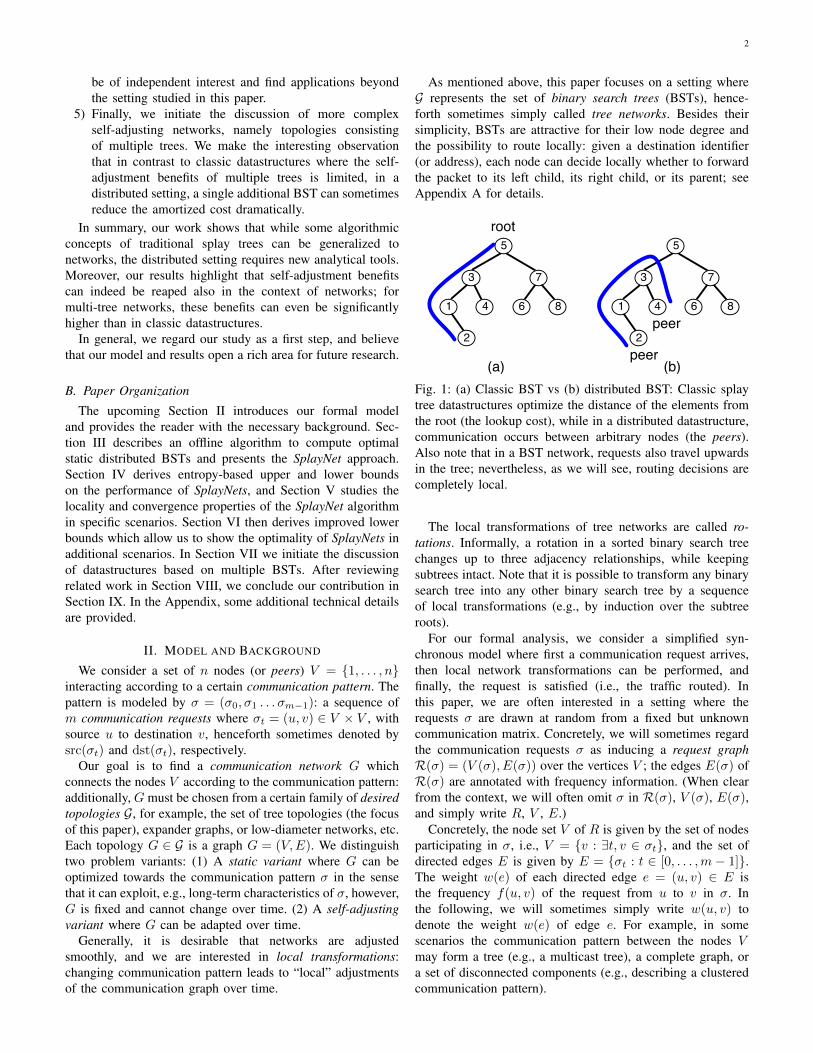
Fig. 2: Basic rotations of splay trees. The dashed bold linesindicate adjacency relationships which are not maintainedduring the operation.

Let A be an algorithm that given the request σt and thegraph Gt ∈ G at time t, transforms the current graph (vialocal transformations) to Gt+1 ∈ G at time t+ 1. We will usethe notation A = ⊥ to refer to a static (i.e., non-adjusting) “al-gorithm” which does not change the communication networkover time.

We are interested in the fundamental tradeoff between thebenefits of self-adjusting algorithms (i.e., shorter routing paths)and their costs (namely reconfiguration costs). We introducea most simple, linear cost model that captures this tradeoff.Concretely, we denote the cost of the network transformationsat time t by ρ(A, Gt, σt), and we denote the number ofrotations performed to change Gt to Gt+1; when A is clearfrom the context, we will simply write ρt. We denote withdG(·) the distance function between nodes in G, i.e., for twonodes v, u ∈ V we define dG(u, v) to be the number of edgesof a shortest path between u and v in G, and we assumemessages are routed along the shortest paths. For a givensequence of communication requests, the cost for an algorithmis given by the number of transformations and the distance ofthe communication requests plus one (i.e., also a request (u, u)comes at a minimal cost of one unit).

We need the following formal definitions.

Definition 1 (Average and Amortized Cost). For an algorithmA and given an initial network G0 with node distance functiond(·) and a sequence σ = (σ0, σ1 . . . σm−1) of communicationrequests over time, we define the (average) cost of A as:

Cost(A, G0, σ) =1

m

m−1∑t=0

(dGt(σt) + 1 + ρt) (1)

The amortized cost of A is defined as the worst possible costof A, i.e., maxG0,σ Cost(A, G0, σ).

Similarly to classic splay trees [22], our yardstick to evalu-ate the obtained costs of a self-adjusting algorithm is the costto serve the same requests σ on an optimal static tree network.

Definition 2 (Optimal Static Cost). The optimal static costfor a given communication sequence σ is defined as the costCost(⊥, G∗, σ) = 1

m

∑m−1t=0 (dG∗(σt) + 1) where ⊥ denotes a

static algorithm that does not change the topology, and G∗ ∈G is the graph in the allowed graph family G that minimizesthe cost with respect to σ.

A. Entropy and Empirical Entropy

The entropy of the communication pattern σ turns out tobe a useful parameter to evaluate the performance of self-adjusting SplayNets. For a discrete random variable X withpossible values x1, . . . , xn, the entropy H(X) of X isdefined as

∑ni=1 p(xi) log2

1p(xi)

where p(xi) is the probabilitythat X takes the value xi. Note that, 0 · log2

10 is considered

as 0. For a joint distribution over X,Y , the joint entropyis defined as H(X,Y ) =

∑i,j p(xi, yj) log2

1p(xi,yj) . Also

recall the definition of the conditional entropy H(X|Y ):H(X|Y ) =

∑nj=1 p(yj)H(X|Y = yj).

Since the sequence of communications σ is revealed overtime and may not be chosen from a fixed probability dis-tribution, we are often interested in the empirical entropyof σ, i.e., the entropy implied by the communication fre-quencies. Let X(σ) = f(x1), . . . , f(xn) be the empiricalentropy measure of the frequency distribution of the com-munication sources (origins) occurring in the communica-tion sequence σ, i.e., f(xi) is the frequency with which anode xi appears as a source in the sequence, i.e., f(xi) =(#xi is a source in σ)/m. The empirical entropy H(X) isthen defined as

∑ni=1 f(xi) log2

1f(xi)

. Similarly, we define theempirical entropy of the communication destinations H(Y )and analogously, the empirical conditional entropies H(X|Y )and H(Y |X).

B. Splay Trees

Our work can be regarded as a distributed generalization ofsplay trees, binary search trees whose topology adapts to thelookup sequence. Indeed, assuming that all requests originatefrom the same node, the SplayNet problem becomes equivalentto the classic splay tree problem. In the following, we hencebriefly review the concept of splay trees.

For a node set V with unique identifiers (IDs) or values,we consider the family B of the set of all binary search treesover the IDs of V . Let s = (v0, v1, . . . , vm−1), vi ∈ V , bea sequence of lookup requests. In the classic offline problem(i.e., for algorithm A = ⊥), the goal is to find the best searchtree T ∗ ∈ B that minimizes the cost Cost(⊥, T ∗, s).

We will make use of the following two well-known prop-erties of optimal BSTs.

Theorem 1 ([16]). An optimal binary search tree T ∗ thatserves s with minimum cost can be found via dynamic pro-gramming.

4

Note however that the computation of T ∗ is more compli-cated than simply using greedy Huffman coding [15] on thefrequency distribution of the items in s.

Theorem 2 ([17]). Given s, for any (optimal) binary searchtree T :

Cost(⊥, T, s) ≥ 1

log 3H(Y ) (2)

where Y (s) is the empirical measure of the frequency distri-bution of s and H(Y ) is its empirical entropy.

Knuth [16] first gave an algorithm to find an optimal BST,but Mehlhorn [17] proved that a simple greedy algorithm isnear optimal with an explicit bound:

Theorem 3 ([17]). Given s, there is a BST which can becomputed using a balancing argument and which has theamortized cost that is at most

Cost(⊥, T, s) ≤ 2 +H(Y )

1− log(√

5− 1)(3)

where Y (s) is the empirical measure of the frequency distri-bution of s and H(Y ) is its empirical entropy.

We can adapt some tools developed for dynamic binarysearch trees also in our generalized setting. In particular, aswe will see, our SplayNet algorithm is a natural generaliza-tion of the splay tree algorithm: it limits operations to thesmallest subtree connecting two communication partners. Thebasic operation to adjust a splay tree is called splaying (seeAlgorithm 1) which consists of the classic Zig, ZigZig, andZigZag rotations. In a nutshell, the main idea of the onlinesplay tree algorithm introduced by Sleator and Tarjan [22]is to rotate (using the uniquely defined sequence of Zig,ZigZig, and ZigZag operations) the currently accessedelement directly to the root of the tree. Interestingly, this ratheraggressive scheme to promote elements already after a singleaccess, results in a good performance.

For our analysis of the distributed setting, we can also adaptthe Access Lemma [22] by Sleator and Tarjan. It is reviewed inthe following. In [22], in order to compute the amortized timeto splay a tree, each node v in the tree is assigned an arbitraryweight w(v). Then the size of a node v, s(v) is defined as thesum of the individual weights of all the nodes in the subtreerooted at v. The so-called rank r(v) of a node v is the logarithmof its size, i.e., r(v) = log(s(v)). Sleator and Tarjan showedthe following:

Lemma 1 (Access Lemma [22]). The amortized timeto splay a tree with root r at a node u is at most3 · (r(r)− r(u)) + 1 = O(log (s(r)/s(u))).

Algorithm 1 Algorithm SPLAY

1: (* upon lookup (u) *)2: splay u to root of T

Following this lemma, Sleator and Tarjan were able to showthat splay trees are optimal with respect to static binary searchtrees:

Theorem 4 (Static Optimality Theorem [22] - rephrased). LetSPLAY denote the SPLAY algorithm. Let s be a sequence oflookup requests where each item is requested at least once,then for any initial tree T , Cost(SPLAY, T, s) = O(H(Y ))where H(Y ) is the empirical entropy of s.

III. SPLAY NETWORKS

We first acquaint ourselves with the distributed BSTmodel by studying optimal static topologies. Subsequently,we present the SplayNet approach and introduce the simpleSPLAYNET algorithm to self-adjust the network.

A. Optimal Static Distributed BST

Given a certain communication pattern or “guest graph”,the optimal BST can be computed in polynomial time usinga dynamic programming approach. The main insight neededis that the problem for the entire tree can be decomposed intooptimal subproblems for smaller trees, and that the demandtowards a given node in a subtree can be decoupled from nodesoutside a given subtree: the precise topological structure of thenodes outside a subtree does not matter.

Concretely, the optimal static tree T which minimizes thesum of the weighted node distances

min∑

(u,v)∈R(σ)

dT (u, v)

can be computed using dynamic programming. Let V denotethe set of ordered nodes and let R denote the request matrix(i.e., the frequency of a given ordered communication pair).We will index subproblems by intervals I on V , and will referto all nodes outside I by I = V \ I . For each node v in aninterval I , we can compute the aggregate demand towards v(v’s weight) from nodes outside I:

WI(v) :=∑u∈I

w(u, v) + w(v, u)

Let WI denote the corresponding vector consisting of all nodesin the interval I .

The demand from outside the considered interval can be“decoupled” with the aggregate weight. The cost of a giventree TI on I can be computed as follows:

Cost(TI ,WI) =

∑u,v∈I

(d(u, v) + 1) · w(u, v)

+DI ·WI

where DI in the scalar product DI ·WI is the vector denotingthe distance of the nodes in I from the root of TI , i.e., thevector of the depths of the nodes.

Dynamic programming is then based on merging optimalsub-intervals. In order to compute the optimal tree T ∗I foran interval I partitioned into two contiguous and adjacentsubintervals I ′ and I ′′, we exploit the computed optimalsubstructures for the sub-intervals and choose the best overallroot x. For the induction hypothesis, a single-node tree has

5

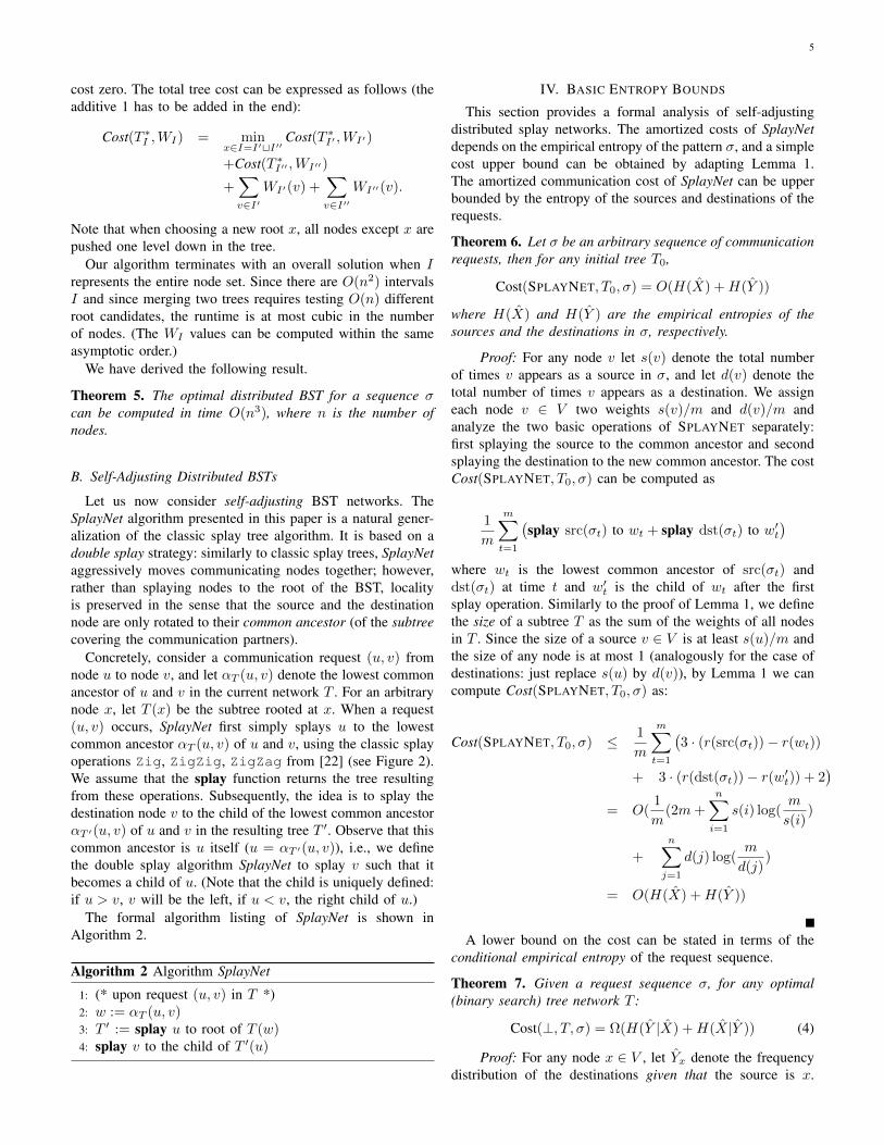
cost zero. The total tree cost can be expressed as follows (theadditive 1 has to be added in the end):

Cost(T ∗I ,WI) = minx∈I=I′tI′′

Cost(T ∗I′ ,WI′)

+Cost(T ∗I′′ ,WI′′)

+∑v∈I′

WI′(v) +∑v∈I′′

WI′′(v).

Note that when choosing a new root x, all nodes except x arepushed one level down in the tree.

Our algorithm terminates with an overall solution when Irepresents the entire node set. Since there are O(n2) intervalsI and since merging two trees requires testing O(n) differentroot candidates, the runtime is at most cubic in the numberof nodes. (The WI values can be computed within the sameasymptotic order.)

We have derived the following result.

Theorem 5. The optimal distributed BST for a sequence σcan be computed in time O(n3), where n is the number ofnodes.

B. Self-Adjusting Distributed BSTs

Let us now consider self-adjusting BST networks. TheSplayNet algorithm presented in this paper is a natural gener-alization of the classic splay tree algorithm. It is based on adouble splay strategy: similarly to classic splay trees, SplayNetaggressively moves communicating nodes together; however,rather than splaying nodes to the root of the BST, localityis preserved in the sense that the source and the destinationnode are only rotated to their common ancestor (of the subtreecovering the communication partners).

Concretely, consider a communication request (u, v) fromnode u to node v, and let αT (u, v) denote the lowest commonancestor of u and v in the current network T . For an arbitrarynode x, let T (x) be the subtree rooted at x. When a request(u, v) occurs, SplayNet first simply splays u to the lowestcommon ancestor αT (u, v) of u and v, using the classic splayoperations Zig, ZigZig, ZigZag from [22] (see Figure 2).We assume that the splay function returns the tree resultingfrom these operations. Subsequently, the idea is to splay thedestination node v to the child of the lowest common ancestorαT ′(u, v) of u and v in the resulting tree T ′. Observe that thiscommon ancestor is u itself (u = αT ′(u, v)), i.e., we definethe double splay algorithm SplayNet to splay v such that itbecomes a child of u. (Note that the child is uniquely defined:if u > v, v will be the left, if u < v, the right child of u.)

The formal algorithm listing of SplayNet is shown inAlgorithm 2.

Algorithm 2 Algorithm SplayNet

1: (* upon request (u, v) in T *)2: w := αT (u, v)3: T ′ := splay u to root of T (w)4: splay v to the child of T ′(u)

IV. BASIC ENTROPY BOUNDS

This section provides a formal analysis of self-adjustingdistributed splay networks. The amortized costs of SplayNetdepends on the empirical entropy of the pattern σ, and a simplecost upper bound can be obtained by adapting Lemma 1.The amortized communication cost of SplayNet can be upperbounded by the entropy of the sources and destinations of therequests.

Theorem 6. Let σ be an arbitrary sequence of communicationrequests, then for any initial tree T0,

Cost(SPLAYNET, T0, σ) = O(H(X) +H(Y ))

where H(X) and H(Y ) are the empirical entropies of thesources and the destinations in σ, respectively.

Proof: For any node v let s(v) denote the total numberof times v appears as a source in σ, and let d(v) denote thetotal number of times v appears as a destination. We assigneach node v ∈ V two weights s(v)/m and d(v)/m andanalyze the two basic operations of SPLAYNET separately:first splaying the source to the common ancestor and secondsplaying the destination to the new common ancestor. The costCost(SPLAYNET, T0, σ) can be computed as

1

m

m∑t=1

(splay src(σt) to wt + splay dst(σt) to w′t

)where wt is the lowest common ancestor of src(σt) anddst(σt) at time t and w′t is the child of wt after the firstsplay operation. Similarly to the proof of Lemma 1, we definethe size of a subtree T as the sum of the weights of all nodesin T . Since the size of a source v ∈ V is at least s(u)/m andthe size of any node is at most 1 (analogously for the case ofdestinations: just replace s(u) by d(v)), by Lemma 1 we cancompute Cost(SPLAYNET, T0, σ) as:

Cost(SPLAYNET, T0, σ) ≤ 1

m

m∑t=1

(3 · (r(src(σt))− r(wt))

+ 3 · (r(dst(σt))− r(w′t)) + 2)

= O(1

m(2m+

n∑i=1

s(i) log(m

s(i))

+

n∑j=1

d(j) log(m

d(j))

= O(H(X) +H(Y ))

A lower bound on the cost can be stated in terms of theconditional empirical entropy of the request sequence.

Theorem 7. Given a request sequence σ, for any optimal(binary search) tree network T :

Cost(⊥, T, σ) = Ω(H(Y |X) +H(X|Y )) (4)

Proof: For any node x ∈ V , let Yx denote the frequencydistribution of the destinations given that the source is x.

6

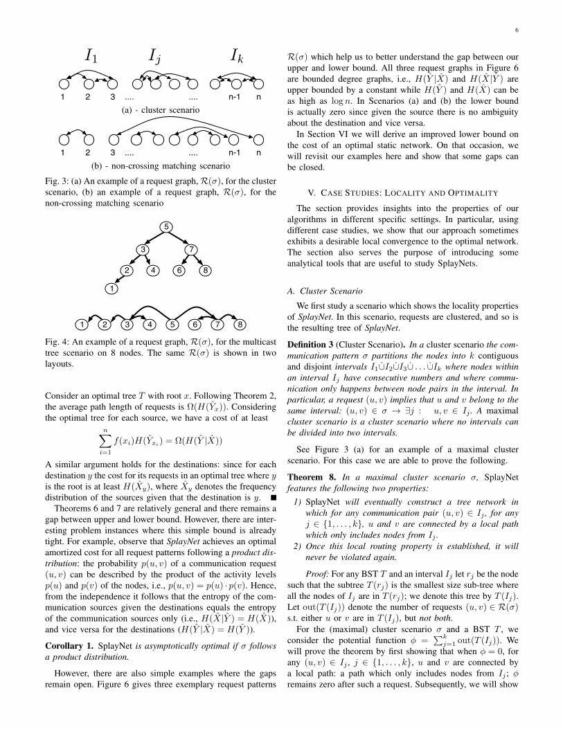
1 2 3 n-1 n........

I1 IkIj

(a) - cluster scenario

1 2 3 n-1 n........(b) - non-crossing matching scenario

Fig. 3: (a) An example of a request graph,R(σ), for the clusterscenario, (b) an example of a request graph, R(σ), for thenon-crossing matching scenario

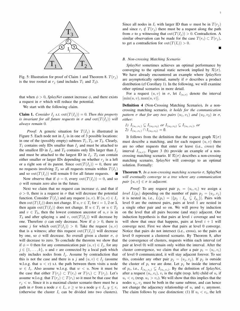
1 2 3 4 5 6 7 8

3

42

1

7

6 8

5

Fig. 4: An example of a request graph, R(σ), for the multicasttree scenario on 8 nodes. The same R(σ) is shown in twolayouts.

Consider an optimal tree T with root x. Following Theorem 2,the average path length of requests is Ω(H(Yx)). Consideringthe optimal tree for each source, we have a cost of at least

n∑i=1

f(xi)H(Yxi) = Ω(H(Y |X))

A similar argument holds for the destinations: since for eachdestination y the cost for its requests in an optimal tree where yis the root is at least H(Xy), where Xy denotes the frequencydistribution of the sources given that the destination is y.

Theorems 6 and 7 are relatively general and there remains agap between upper and lower bound. However, there are inter-esting problem instances where this simple bound is alreadytight. For example, observe that SplayNet achieves an optimalamortized cost for all request patterns following a product dis-tribution: the probability p(u, v) of a communication request(u, v) can be described by the product of the activity levelsp(u) and p(v) of the nodes, i.e., p(u, v) = p(u) · p(v). Hence,from the independence it follows that the entropy of the com-munication sources given the destinations equals the entropyof the communication sources only (i.e., H(X|Y ) = H(X)),and vice versa for the destinations (H(Y |X) = H(Y )).

Corollary 1. SplayNet is asymptotically optimal if σ followsa product distribution.

However, there are also simple examples where the gapsremain open. Figure 6 gives three exemplary request patterns

R(σ) which help us to better understand the gap between ourupper and lower bound. All three request graphs in Figure 6are bounded degree graphs, i.e., H(Y |X) and H(X|Y ) areupper bounded by a constant while H(Y ) and H(X) can beas high as log n. In Scenarios (a) and (b) the lower boundis actually zero since given the source there is no ambiguityabout the destination and vice versa.

In Section VI we will derive an improved lower bound onthe cost of an optimal static network. On that occasion, wewill revisit our examples here and show that some gaps canbe closed.

V. CASE STUDIES: LOCALITY AND OPTIMALITY

The section provides insights into the properties of ouralgorithms in different specific settings. In particular, usingdifferent case studies, we show that our approach sometimesexhibits a desirable local convergence to the optimal network.The section also serves the purpose of introducing someanalytical tools that are useful to study SplayNets.

A. Cluster Scenario

We first study a scenario which shows the locality propertiesof SplayNet. In this scenario, requests are clustered, and so isthe resulting tree of SplayNet.

Definition 3 (Cluster Scenario). In a cluster scenario the com-munication pattern σ partitions the nodes into k contiguousand disjoint intervals I1∪I2∪I3∪ . . . ∪Ik where nodes withinan interval Ij have consecutive numbers and where commu-nication only happens between node pairs in the interval. Inparticular, a request (u, v) implies that u and v belong to thesame interval: (u, v) ∈ σ → ∃j : u, v ∈ Ij . A maximalcluster scenario is a cluster scenario where no intervals canbe divided into two intervals.

See Figure 3 (a) for an example of a maximal clusterscenario. For this case we are able to prove the following.

Theorem 8. In a maximal cluster scenario σ, SplayNetfeatures the following two properties:

1) SplayNet will eventually construct a tree network inwhich for any communication pair (u, v) ∈ Ij , for anyj ∈ 1, . . . , k, u and v are connected by a local pathwhich only includes nodes from Ij .

2) Once this local routing property is established, it willnever be violated again.

Proof: For any BST T and an interval Ij let rj be the nodesuch that the subtree T (rj) is the smallest size sub-tree whereall the nodes of Ij are in T (rj); we denote this tree by T (Ij).Let out(T (Ij)) denote the number of requests (u, v) ∈ R(σ)s.t. either u or v are in T (Ij), but not both.

For the (maximal) cluster scenario σ and a BST T , weconsider the potential function φ =

∑kj=1 out(T (Ij)). We

will prove the theorem by first showing that when φ = 0, forany (u, v) ∈ Ij , j ∈ 1, . . . , k, u and v are connected bya local path: a path which only includes nodes from Ij ; φremains zero after such a request. Subsequently, we will show

7

T1 T2

T3

x y

rj

Ij

Fig. 5: Illustration for proof of Claim 1 and Theorem 8. T (rj)is the tree rooted at rj (and includes T1 and T2).

that when φ > 0, SplayNet cannot increase φ, and there existsa request in σ which will reduce the potential.

We start with the following claim.

Claim 1. Consider Ij s.t. out(T (Ij)) = 0. Then this propertyis invariant for all future requests in σ and out(T (Ij)) willalways remain 0.

Proof: A generic situation for T (Ij) is illustrated inFigure 5. Each node not in Ij is in one of 3 possible locations:in one of the (possibly empty) subtrees T1, T2, or T3. Clearly,T1 contains only IDs smaller than Ij and must be attached tothe smallest ID in Ij , and T2 contains only IDs larger than Ijand must be attached to the largest ID in Ij . T3 can containeither smaller or larger IDs depending on whether rj is a leftor a right son of its parent. Since out(T (Ij)) = 0, there areno requests involving T3 so all requests remain within T (Ij)and so out(T (Ij)) will remain 0 for all future requests.

Now observe that if φ = 0, every out(T (Ij)) = 0, and soφ will remain zero also in the future.

Next we claim that no request can increase φ, and that ifφ > 0, there is a request in σ that will decrease the potentialfunction. Consider T (Ij) and any request (u, v). If (u, v) ∈ Ijthen out(T (Ij)) does not change. If u, v ∈ Ti for i = 1, 2 or 3,then again out(T (Ij)) does not change. If u ∈ T1 or u ∈ T2

and v ∈ T3, then the lowest common ancestor of u, v is inT3 and after splaying u and v, out(T (Ij)) will decrease byone. Therefore φ can only decrease. Now if φ > 0, there issome j for which out(T (Ij)) > 0. Take the request (u, v)that is a witness; after this request out(T (Ij)) will decreaseby one, so φ will decrease. So overall given a cluster σ, φwill decrease to zero. To conclude the theorem we show thatif φ = 0 then for any communication pair (u, v) ∈ Ij , for anyj ∈ 1, . . . , k, u and v are connected by a local path whichonly includes nodes from Ij . Assume by contradiction thatthis is not the case and there is a j and (u, v) ∈ Ij (assumew.l.o.g. that u < v) s.t. the path between them visits a nodew ∈ Ii. Also assume w.l.o.g. that w < u. Now it must bethe case that either T (rj) ⊂ T (ri) or T (ri) ⊂ T (rj). Let’sassume w.l.o.g. that T (rj) ⊂ T (ri) so it must be that case thatrj < w. Since it is a maximal cluster scenario there must be apath in σ from a node x ∈ Ii, x ≥ w to a node y ∈ Ii, y ≤ ri(otherwise the cluster Ii can be divided into two clusters).

Since all nodes in Ii with larger ID than w must be in T (rj)and since ri /∈ T (rj) there must be a request along the pathfrom x to y witnessing that out(T (Ij)) > 0. Contradiction. Asimilar observation can be made for the case T (ri) ⊂ T (rj),to get a contradiction for out(T (Ii)) > 0.

B. Non-crossing Matching Scenario

SplayNet sometimes achieves an optimal performance byconverging to the optimal static network implied by R(σ).We have already encountered an example where SplayNetsare asymptotically optimal, namely if σ describes a productdistribution (cf Corollary 1). In the following, we will examineother optimal scenarios in more detail.

For a request (u, v) in σ, let I(u,v) denote the interval[min(u, v),max(u, v)].

Definition 4 (Non-Crossing Matching Scenario). In a non-crossing matching scenario, it holds for the communicationpattern σ that for any two pairs (u1, v1) and (u2, v2) in σ,either:

1) I(u1,v1) ( I(u2,v2) or I(u2,v2) ( I(u1,v1), or2) I(u1,v1) ∩ I(u2,v2) = ∅.

It follows from the definition that the request graph R(σ)must describe a matching, and for each request (u, v) thereare no other requests that enter or leave (i.e., cross) theinterval I(u,v). Figure 3 (b) provide an example of a non-crossing matching scenario. If R(σ) describes a non-crossingmatching scenario, SplayNet will converge to an optimalsolution. Formally:

Theorem 9. In a non-crossing matching scenario σ, SplayNetwill eventually converge to a tree where any communicationpair u, v ∈ σ is adjacent.

Proof: To any request pair pi = (ui, vi) we assign alevel L(pi) depending on the number of pairs pj = (uj , vj)it is nested in, i.e., L(pi) = |pj : Ipi ( Ipj|. Pairs withlevel 0 are the outmost pairs, pairs at level 1 are nested ina single other pair and so on. We will prove by inductionon the level that all pairs become (and stay) adjacent. Ourinduction hypothesis is that pairs at level i coverage and wewill show that once that happens, pairs at level i + 1 willconverge next. First we show that pairs at level 0 converge.Notice that pairs do not intersect (i.e., cross), so the pairs atlevel 0 represent a clustered scenario. By Theorem 8, afterthe convergence of clusters, requests within each interval (ofpair at level 0) will remain only within the interval. After thecluster convergence, we claim that after a pair pi = (ui, vi)of level 0 communicated, it will stay adjacent forever. To seethis, consider any other pair pj = (uj , vj). If pj is outsidethe cluster of pi we are done. Let pj be inside the intervalof pi, i.e., I(uj ,vj) ( I(ui,vi). By the definition of SplayNet,after a request (ui, vi), vi is the right (resp. left) child of ui ifui < vi (resp. u1 > v1). We will show that this implies that thenodes uj , vj must be both in the same subtree, and can hencenot change the adjacency relationship of ui and vi anymore.The claim follows by case distinction: (1) If ui < vi, the left

8

subtree of vi is the only subtree which can contain nodes wwith ui < w < vi; however, these are exactly the nodes thatcan fulfill the non crossing property so both uj and vj mustbe in this subtree. If ui > vi, the right subtree of vi is theonly subtree which can contain nodes w with u1 < w < v1 soboth uj and vj must be in this subtree. Therefore the inductionhypothesis holds for level 0.

We can now prove the induction step. Assume the links oflevel up to i are stable. Note that within each cluster the pairsof level i + 1 are also disjoint and correspond to a clusteredscenario. Essentially, then the previous argument still holds,and first each cluster of levels larger than i will converge,by Theorem 8, and then, after a pair from level i + 1 willcommunicate, it will never break apart again since all higherlevel pairs are in the same subtree.

C. Multicast Scenario

To give one more example where SplayNet is optimal, weconsider the multicast tree scenario. For this scenario, wemay assume that an overlay network of a binary search treestructure is constructed to facilitate in-network duplication.The same tree may be used by many multicast sourcesand different receivers, hence the local (hop-by-hop) sourceand destination pairs (i.e., communication requests) are theendpoints of the tree edges.

Definition 5 (Binary Multicast Tree Scenario). In a binarymulticast tree scenario, it holds for the communication patternσ that the request graph R(σ) forms a rooted and sortedbinary tree.

See Figure 4 for an example of a multicast scenario. Forthis case as well, we are able to prove optimality.

Theorem 10. If the communication pairs in σ form a multicasttree, SplayNet will eventually converge to the optimal staticsolution, i.e., to R(σ).

Proof: Let T (v) denote the subtree of v (including v)in the current SplayNet, and let Tl(v) and Tr(v) denote v’sleft and right subtree, respectively. Similarly, let R(v) denotethe subtree of v in the multicast tree R(σ), and let Rl(v)resp. Rr(v) denote the left resp. right subtree. Consider thepath from the root of R(σ), denoted by vi, to the maximumnode in R(σ), denoted by v1, and let this path be Pm =vi, . . . , v2, v1, where for j = 1, . . . , i, vj is the parent of vj−1.

We start with a fundamental invariant.

Claim 2. Let vj ∈ Pm denote a node in the path from the rootto the maximum node. Then it holds that once T (vj) = R(vj),the parent of vj in T will be vj+1. These properties will remaininvariant during all future requests.

Proof: We first prove the identical parent property. If j =i the result holds trivially since T and R(σ) are identical. Letj < i. For the sake of contradiction, assume that T (vj) =R(vj), that the parent of vj inR(σ) is vj+1, but that the parentof v in T is x 6= vj+1. It holds that vj+1 < vj . Since bothT and R are valid BSTs, x cannot be in the subtree T (vj) =R(vj), and it must hold that vj+1 < x < vj . However, the

fact that vj+1 is a parent of vj in R(σ) implies that x must bea decedent of vj in R(σ), which contradicts our assumptionthat T (vj) = R(vj).

It remains to show that the trees will also remain the same inthe future. Consider any future request (y, z). Since T (vj) =R(vj) and there are no requests leaving R(vj) beside vj andits parent, vj cannot be on a path between y to z (whichincludes their least common ancestor), and hence, T (vj) willremain unchanged during any splay operation.

We can also make the following observation.

Claim 3. Let vj ∈ Pm denote a node in the path fromthe root to the maximum node for j < i. Once the rightsubtrees Tr(vj−1) and Rr(vj−1) of the node vj are the same,then after a request (vj+1, vj) from vj’s parent in R(σ) thesubtree Tl(vj) will have exactly the same nodes as Rl(vj).This property will remain invariant during all future requests.

Proof: Assume T (vj−1) = Rr(vj−1). Then by Claim 2,vj is the parent of vj−1 in T , and this still holds afterthe request (vj+1, vj). Recall that vj+1 < vj and we areconsidering the right most tree branch. However, this impliesthat all the nodes between vj+1 and vj must be situated in thesame subtree, the left subtree of vj So Tl(vj) will have theexact same nodes as Rl(vj).

Now consider any future request (y, z). Since T (vj) andR(vj) have now the same set of nodes, vj is not on a pathbetween y to z (which includes their least common ancestor),so T (vj) will indeed remain unchanged during such a request.

We are now ready to prove the theorem by induction overthe number of nodes. That is, we will show that for each sizek of R(σ), the theorem holds.

Induction Base: The claim trivially holds for the caseswhere we only have one node (k = 1) or one request (k = 2).

Induction Step: Assume that the hypothesis is true for1, . . . , k−1; we will now show that it is also true for k nodes.We will prove, again by induction, but now on j, that T (vj)will become (and stay) R(vj): one node after the other alongthis path will stabilize.

Base case, j = 1: Since v1 is the maximum node it has noright child both in T and R(σ). By Claim 3 after therequest (v2, v1) T (v1) and R(v1) will have the same setof nodes. Since R(v1) has less than k nodes by the maininduction hypothesis we will eventually have T (v1) =R(v1).

Induction step: Assume the claim is true for j − 1. If j < ithen after the request (vj , vj−1), by Claim 3 Tl(vj) willconsist of the same nodes as Rl(vj), and by the maininduction hypothesis (since the size of Rl(vj) < k) andClaim 3, Tl(vj) will converge to Rl(vj). Then we willhave T (vj) = R(vj).

To prove the claim also holds for the root, we can simplyapply a variant of Claim 3 also to a path from the root to theminimum node. Given that both subtrees of the root stabilize,also the root will be stabilized.

9

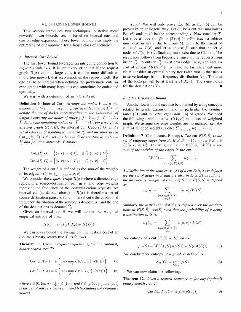
VI. IMPROVED LOWER BOUNDS

This section introduces two techniques to derive morepowerful lower bounds: one is based on interval cuts andone on edge expansion. These lower bounds also imply theoptimality of our approach for a larger class of scenarios.

A. Interval Cuts Bound

The first lower bound leverages an intriguing connection torequest graph cuts. It is intuitively clear that if the requestgraph R(σ) exhibits large cuts, it can be more difficult tofind a tree network that accommodates the requests well. Butone has to be careful when defining the problematic cuts, aseven graphs with many large cuts can sometimes be embeddedoptimally.

We start with a definition of an interval cut.

Definition 6 (Interval Cut). Arrange the nodes V on a onedimensional line in an ascending, sorted order, and let I`j ⊆ Vdenote the set of nodes corresponding to the subinterval oflength ` covering the nodes of order j, j+ 1, ..., j+ `− 1. LetI`j denote the remaining nodes, i.e., I`j = V \I`j . For a weighteddirected graph G(V,E), the interval cut, Cutin(I`j , G) is theset of edges in G pointing to nodes in I`j , and the interval cutCutout(I

`j , G) is the set of edges in G originating at nodes in

I`j and pointing outwards. Formally

Cutin(I`j , G) =

(u, v) : v ∈ I`j , u ∈ I`j , (u, v) ∈ G

Cutout(I

`j , G) =

(u, v) : u ∈ I`j , v ∈ I`j , (u, v) ∈ G

The weight of a cut c is defined as the sum of the weights

of its edges, w(c) =∑

(u,v)∈c w(u, v).

We consider the request graph R(σ) where a directed edgerepresent a source-destination pair in σ and edge weightsrepresent the frequency of the communication requests. Aninterval cut (as defined above) in R(σ) is therefor a set ofsource-destination pairs, so for an interval cut c the conditionalfrequency distribution of the sources is denoted Xc and the oneof the destinations is denoted Yc.

Given an interval cut c, we will denote the weightedempirical entropy of c as:

H(c) = w(c)(H(Xc) +H(Yc)

)We can lower bound the average communication cost of an

(optimal) binary search tree T as follows.

Theorem 11. Given a request sequence σ, for any (optimal)binary search tree T :

Cost(⊥, T, σ) = Ω

(max

iminj,`

H(Cutin(I`j ,R(σ)))

)(5)

Cost(⊥, T, σ) = Ω

(max

iminj,`

H(Cutout(I`j ,R(σ)))

)(6)

where i ∈ [0, log n−1], j ∈ [1, n] and ` ∈ [ n2i+1 ,

n2i ] and [a, b]

is the set of integers between a and b (including the boundarynodes).

Proof: We will only prove Eq. (6), as Eq. (5) can beproved in an analogous way. Let c∗, be a cut that maximizesEq. (6) and let i∗ be the corresponding i. Now consider T .Let v be a node s.t. n

2i∗ > |T (v)| ≥ n2i∗+1 (such a subtree

must exist in any T due to Claim 5). Let u be the parent ofv. Let `∗ = |T (v)| and let us choose j∗ such that the set ofnodes of T (v) is I`

∗

j∗ . Such a j must exist due to Claim 4. Theresult now follows from Property 2, since all the requests frominside I`

∗

j∗ to outside I`∗

j∗ must cross edge (u, v) and entail acost of at least Ω(H(c∗)). To make the last statement moreclear, consider an optimal binary tree (with root v) that needsto serve lookups from a frequency distribution Xc∗ . The costof the lookups will be at least Ω(H(Xc∗)). The same holdsfor the destinations Yc∗ .

B. Edge Expansion Bound

Another lower bound can also be obtained by using conceptsrelated to graph expansion, and in particular the conduc-tance [21] and the edge expansion [14] of graphs. We needthe following definitions: Let G(V,E) be a directed weightedgraph. We assume the edge weights are normalized, i.e., thesum of all edge weights is one:

∑(u,v)∈E w(u, v) = 1.

Definition 7 (Conductance Entropy). The cut E(S, S) is theset of outgoing edges from S: E(S, S) = (u, v) : u ∈ S, v ∈S, (u, v) ∈ E. The weight of a cut E(S, S), W (S) is thesum of the weights of the edges in the cut.

W (S) =∑

(u,v)∈E(S,S)

w(u, v)

A distribution of the sources src(S) of a cut E(S, S) is definedfor the set of nodes in S that are also in E(S, S) as follows:the probability (weight) of each u ∈ S and E(S, S) is definedas

wS(u) =∑

(u,v)∈E(S,S)u∈S

w(u, v)/W (S).

Similarly the distribution dst(S) is defined over the destina-tions in E(S, S), src(S) such that the probability of v beinga destination in S is:

wS(v) =∑

(u,v)∈E(S,S)v∈S

w(u, v)/W (S).

The entropy of a cut (S, S) is defined as:

ϕH(S) = W (S) (H(src(S)) +H(dst(S))) (7)

The conductance entropy of a graph is defined as:

φH(G) = minS⊆V

ϕ(S) (8)

We can now claim the following:

Theorem 12. Given a request sequence σ, for any (optimal)binary search tree T :

Cost(⊥, T, σ) = Ω(φH(R(σ))) (9)

10

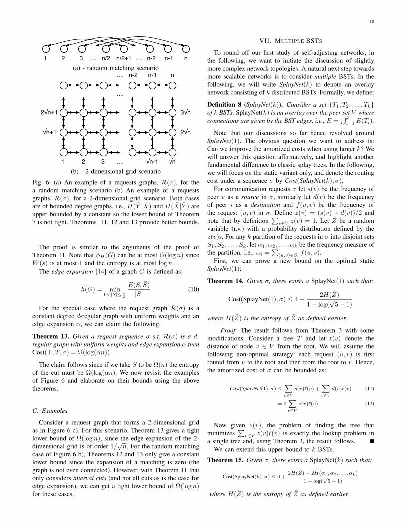
1 2 3 n/2 n/2+1 n-1 n........ n-2(a) - random matching scenario

1 2 3 √n-1 √n

n-1 n

....

....

....

n-2

√n+1 2√n

3√n2√n+1

(b) - 2-dimensional grid scenario

Fig. 6: (a) An example of a requests graphs, R(σ), for thea random matching scenario (b) An example of a requestsgraphs, R(σ), for a 2-dimensional grid scenario. Both casesare of bounded degree graphs, i.e., H(Y |X) and H(X|Y ) areupper bounded by a constant so the lower bound of Theorem7 is not tight. Theorems 11, 12 and 13 provide better bounds.

The proof is similar to the arguments of the proof ofTheorem 11. Note that φH(G) can be at most O(log n) sinceW (s) is at most 1 and the entropy is at most log n.

The edge expansion [14] of a graph G is defined as:

h(G) = min0<|S|≤n

2

E(S, S)

|S|(10)

For the special case where the request graph R(σ) is aconstant degree d-regular graph with uniform weights and anedge expansion α, we can claim the following.

Theorem 13. Given a request sequence σ s.t. R(σ) is a d-regular graph with uniform weights and edge expansion α thenCost(⊥, T, σ) = Ω(log(αn)).

The claim follows since if we take S to be Ω(n) the entropyof the cut must be Ω(log(αn). We now revisit the examplesof Figure 6 and elaborate on their bounds using the abovetheorems.

C. Examples

Consider a request graph that forms a 2-dimensional gridas in Figure 6 c). For this scenario, Theorem 13 gives a tightlower bound of Ω(log n), since the edge expansion of the 2-dimensional grid is of order 1/

√n. For the random matching

case of Figure 6 b), Theorems 12 and 13 only give a constantlower bound since the expansion of a matching is zero (thegraph is not even connected). However, with Theorem 11 thatonly considers interval cuts (and not all cuts as is the case foredge expansion), we can get a tight lower bound of Ω(log n)for these cases.

VII. MULTIPLE BSTS

To round off our first study of self-adjusting networks, inthe following, we want to initiate the discussion of slightlymore complex network topologies. A natural next step towardsmore scalable networks is to consider multiple BSTs. In thefollowing, we will write SplayNet(k) to denote an overlaynetwork consisting of k distributed BSTs. Formally, we define:

Definition 8 (SplayNet(k)). Consider a set T1, T2, . . . , Tkof k BSTs. SplayNet(k) is an overlay over the peer set V whereconnections are given by the BST edges, i.e., E =

⋃ki=1E(Ti).

Note that our discussions so far hence revolved aroundSplayNet(1). The obvious question we want to address is:Can we improve the amortized costs when using larger k? Wewill answer this question affirmatively, and highlight anotherfundamental difference to classic splay trees. In the following,we will focus on the static variant only, and denote the routingcost under a sequence σ by Cost(SplayNet(k), σ).

For communication requests σ let s(v) be the frequency ofpeer v as a source in σ, similarly let d(v) be the frequencyof peer i as a destination and f(u, v) be the frequency ofthe request (u, v) in σ. Define z(v) = (s(v) + d(v))/2 andnote that by definition

∑v∈V z(v) = 1. Let Z be a random

variable (r.v.) with a probability distribution defined by thez(v)s. For any k partition of the requests in σ into disjoint setsS1, S2, . . . , Sk, let α1, α2, . . . , αk be the frequency measure ofthe partition, i.e., αi =

∑(u,v)∈Si

f(u, v).First, we can prove a new bound on the optimal static

SplayNet(1):

Theorem 14. Given σ, there exists a SplayNet(1) such that:

Cost(SplayNet(1), σ) ≤ 4 +2H(Z)

1− log(√

5− 1)

where H(Z) is the entropy of Z as defined earlier.

Proof: The result follows from Theorem 3 with somemodifications. Consider a tree T and let `(v) denote thedistance of node v ∈ V from the root. We will assume thefollowing non-optimal strategy: each request (u, v) is firstrouted from u to the root and then from the root to v. Hence,the amortized cost of σ can be bounded as:

Cost(SplayNet(1), σ) ≤∑v∈V

s(v)`(v) +∑v∈V

d(v)`(v) (11)

= 2∑v∈V

z(v)`(v). (12)

Now given z(v), the problem of finding the tree thatminimizes

∑v∈V z(v)`(v) is exactly the lookup problem in

a single tree and, using Theorem 3, the result follows.We can extend this upper bound to k BSTs.

Theorem 15. Given σ, there exists a SplayNet(k) such that:

Cost(SplayNet(k), σ) ≤ 4 +2H(Z)− 2H(α1, α2, . . . , αk)

1− log(√5− 1)

where H(Z) is the entropy of Z as defined earlier.

11

Proof: Assume a non-optimal strategy where we partitionσ into k disjoint sets of requests S1, S2, . . . , Sk, and eachrequest is routed on its unique BST. In each tree we use theprevious method, and the messages are routed from the sourceto the root and from the root to the destination. For a subsetSi, 1 ≤ i ≤ k, let Zi denote the frequency measure definedas Z, but limited to the requests in Si. Now:

Cost(SplayNet(k), σ) ≤k∑

i=1

αi

(4 + 2

H(Zi)

1− log(√5− 1)

)(13)

= 4 +2

1− log(√5− 1)

k∑i=1

αiH(Zi) (14)

= 4 +2

1− log(√5− 1)

(H(Y )−H(α1, α2, . . . , αk)

)(15)

where the last step is based on the decomposition property ofentropy.

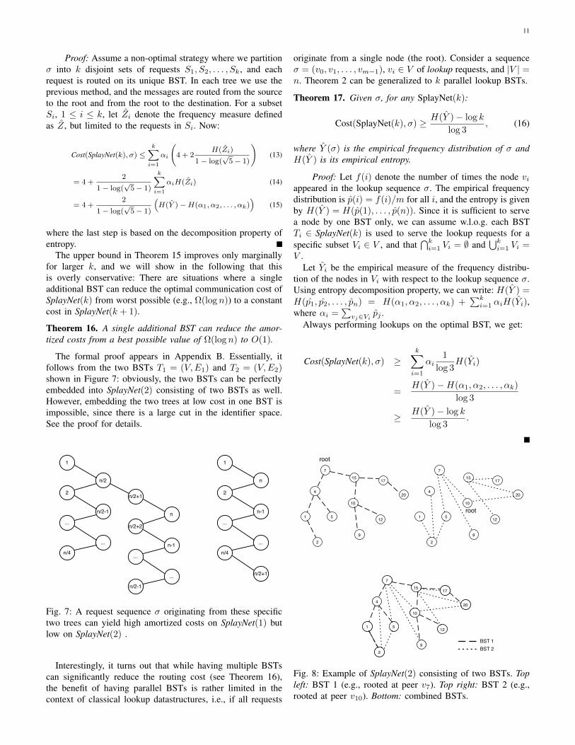
The upper bound in Theorem 15 improves only marginallyfor larger k, and we will show in the following that thisis overly conservative: There are situations where a singleadditional BST can reduce the optimal communication cost ofSplayNet(k) from worst possible (e.g., Ω(log n)) to a constantcost in SplayNet(k + 1).

Theorem 16. A single additional BST can reduce the amor-tized costs from a best possible value of Ω(log n) to O(1).

The formal proof appears in Appendix B. Essentially, itfollows from the two BSTs T1 = (V,E1) and T2 = (V,E2)shown in Figure 7: obviously, the two BSTs can be perfectlyembedded into SplayNet(2) consisting of two BSTs as well.However, embedding the two trees at low cost in one BST isimpossible, since there is a large cut in the identifier space.See the proof for details.

1

2

...

n/4

n/2

n/2-1

...

n/2+1

n/2+2

...

n/2-1

n

n-1

...

1

2

...

n/4

n

n-1

...

n/2+1

Fig. 7: A request sequence σ originating from these specifictwo trees can yield high amortized costs on SplayNet(1) butlow on SplayNet(2) .

Interestingly, it turns out that while having multiple BSTscan significantly reduce the routing cost (see Theorem 16),the benefit of having parallel BSTs is rather limited in thecontext of classical lookup datastructures, i.e., if all requests

originate from a single node (the root). Consider a sequenceσ = (v0, v1, . . . , vm−1), vi ∈ V of lookup requests, and |V | =n. Theorem 2 can be generalized to k parallel lookup BSTs.

Theorem 17. Given σ, for any SplayNet(k):

Cost(SplayNet(k), σ) ≥ H(Y )− log k

log 3, (16)

where Y (σ) is the empirical frequency distribution of σ andH(Y ) is its empirical entropy.

Proof: Let f(i) denote the number of times the node viappeared in the lookup sequence σ. The empirical frequencydistribution is p(i) = f(i)/m for all i, and the entropy is givenby H(Y ) = H(p(1), . . . , p(n)). Since it is sufficient to servea node by one BST only, we can assume w.l.o.g. each BSTTi ∈ SplayNet(k) is used to serve the lookup requests for aspecific subset Vi ∈ V , and that

⋂ki=1 Vi = ∅ and

⋃ki=1 Vi =

V .Let Yi be the empirical measure of the frequency distribu-

tion of the nodes in Vi with respect to the lookup sequence σ.Using entropy decomposition property, we can write: H(Y ) =H(p1, p2, . . . , pn) = H(α1, α2, . . . , αk) +

∑ki=1 αiH(Yi),

where αi =∑vj∈Vi

pj .Always performing lookups on the optimal BST, we get:

Cost(SplayNet(k), σ) ≥k∑i=1

αi1

log 3H(Yi)

=H(Y )−H(α1, α2, . . . , αk)

log 3

≥ H(Y )− log k

log 3.

7

10

1

2

4

15

5

17

12

9

20

7

10

1

2

4

15

5

17

12

9

20

root

7

10

1

2

4

15

5

17

12

9

20

7

10

1

2

4

15

5

17

12

9

20

BST 1BST 2

root

Fig. 8: Example of SplayNet(2) consisting of two BSTs. Topleft: BST 1 (e.g., rooted at peer v7). Top right: BST 2 (e.g.,rooted at peer v10). Bottom: combined BSTs.

12

7

10

1

2

4

15

5

17

12

9

20

7

10

1

2

4

15

5

17

12

9

20

BST 1(root 7)

BST 2(root 10)

LCA(5,12)

Fig. 9: Example for splay operation in SplayNet(2) of Figure 8.

Finally, we sketch an intuitive approach to makeSplayNet(k) self-adjusting: initially, for each BST, we connectall nodes V at random and independently (see Figure 8 for anexample). When communication requests occur, BSTs start toadapt: upon a communication request (u, v), we determinethe BST T where u and v are closest (in case multiple treesyield similar cost, an arbitrary one is taken), as well as theleast common ancestor w of u and v in T : w := αT (u, v).Subsequently, u and v are splayed to the root of the subtree ofT rooted at w, using our SplayNet procedure. Figure 9 gives anexample: upon a communication request between peers v5 andv12, the two peers are splayed to their least common ancestor,peer v7, in BST T1.

VIII. RELATED WORK

Our work builds upon classic literature on self-adaptingdatastructures, and in particular upon the work of Sleatorand Tarjan on splay trees [22]. Since this seminal work,splay trees and their variants (e.g., Tango trees [7] or multi-splay trees [23]) have been studied intensively for many years(e.g. [1], [22]). Moreover, the related dynamic optimalityconjecture [7], [23] is arguably one of the most interestingopen problems in Theoretical Computer Science.

In contrast to the classical splay tree datastructures, ourpaper studies a distributed variant where “lookups” or requestscannot only originate from a single root, but where commu-nication happens between all pairs of nodes in the network.Hence, this paper is situated in the realm of distributeddatastructures or networking.

The static variant of our problem can be seen as a graphembedding [8] or network design [10] problem. In particular,the problem of computing the optimal static network, that is,the binary search tree that minimizes the communication cost,is related to the classic Minimum Linear Arrangement (MLA)problem which asks for the embedding of an arbitrary “guestgraph” on the line: the nodes of the guest graph must bemapped to the line such that the communication cost, i.e., thesum of the lengths of the projected edges, is minimized. Incontrast to the MLA problem, in our case, we need to embedthe guest graph on a binary tree which respects a searchable

order. MLA [9] was originally introduced by Harper [12] inthe context of error-correcting codes with minimal averageabsolute errors, and later used in many other domains suchas for modeling of some nervous activity in the cortex [18]or job scheduling [19]. While there exist many interestingalgorithms for this problem already, e.g., with sublogarithmicapproximation ratios [11] or polynomial-time executions forspecial requests graphs [9], no non-trivial results are knownabout distributed and local solutions.

Bibliographic Note. Preliminary versions of the resultspresented in this paper appeared at DISC 2012 [20], IEEEIPDPS 2013 [6], and IEEE P2P 2013 [4].

IX. CONCLUSION

We regard our work as a first step towards the design ofnovel distributed datastructures and networks which adapt dy-namically to the demand. In order to focus on the fundamentaltradeoff between benefit and cost of self-adjustments, we pur-posefully presented our model in a general and abstract form,and many additional and application-specific aspects need tobe addressed before our approach can be tested in the wild.The main theoretical simplification made in this paper regardsthe restriction to the tree topology, and the generalization tomore complex and redundant networks is an open question.Moreover, similarly to [22], we have focused on the amortizedcosts of SplayNets, and an interesting direction for futureresearch regards the study of the achievable competitive ratiounder arbitrary communication patterns.

REFERENCES

[1] B. Allen and I. Munro. Self-organizing binary search trees. J. ACM,25:526–535, 1978.

[2] J. Aspnes and G. Shah. Skip graphs. ACM Transactions on Algorithms(TALG), 3(4):37–es, 2007.

[3] C. Avin, M. Borokhovich, and S. Schmid. Obst: A self-adjusting peer-to-peer overlay based on multiple bsts. In Peer-to-Peer Computing (P2P),2013 IEEE Thirteenth International Conference on, pages 1–5. IEEE,2013.

[4] C. Avin, M. Borokhovich, and S. Schmid. Obst: A self-adjusting peer-to-peer overlay based on multiple bsts. In Proc. 13th IEEE InternationalConference on Peer-to-Peer Computing (P2P), September 2013.

[5] C. Avin, B. Haeupler, Z. Lotker, C. Scheideler, and S. Schmid. Locallyself-adjusting tree networks. In Parallel & Distributed Processing(IPDPS), 2013 IEEE 27th International Symposium on, pages 395–406.IEEE, 2013.

[6] C. Avin, B. Haeupler, Z. Lotker, C. Scheideler, and S. Schmid. Locallyself-adjusting tree networks. In Proc. 27th IEEE International Paralleland Distributed Processing Symposium (IPDPS), May 2013.

[7] E. D. Demaine, D. Harmon, J. Iacono, and M. Patrascu. Dynamicoptimality - almost. In Proc. 45th Annual IEEE Symposium onFoundations of Computer Science (FOCS), pages 484–490, 2004.

[8] J. Dıaz, J. Petit, and M. Serna. A survey of graph layout problems.ACM Comput. Surv., 34(3):313–356, 2002.

[9] J. Dıaz, J. Petit, and M. Serna. A survey of graph layout problems.ACM Comput. Surv., 34(3):313–356, 2002.

[10] H. Farvaresh and M. Sepehri. A branch and bound algorithm for bi-level discrete network design problem. Networks and Spatial Economics,13(1):67–106, 2013.

[11] U. Feige and J. Lee. An improved approximation ratio for the minimumlinear arrangement problem. Information Processing Letters, 101(1):26–29, 2007.

[12] L. H. Harper. Optimal assignment of numbers to vertices. J. SIAM,(12):131–135, 1964.

[13] N. J. A. Harvey, M. B. Jones, S. Saroiu, M. Theimer, and A. Wolman.Skipnet: A scalable overlay network with practical locality properties. InProc. 4th Conference on USENIX Symposium on Internet Technologiesand Systems (USITS), 2003.

13

[14] S. Hoory, N. Linial, and A. Wigderson. Expander graphs and theirapplications. Bulletin of the American Mathematical Society, 43(4):439–562, 2006.

[15] D. Huffman. A method for the construction of minimum-redundancycodes. Proceedings of the IRE, 40(9):1098–1101, 1952.

[16] D. Knuth. Optimum binary search trees. Acta informatica, 1(1):14–25,1971.

[17] K. Mehlhorn. Nearly optimal binary search trees. Acta Informatica,5(4):287–295, 1975.

[18] G. Mitchison and R. Durbin. Optimal numberings of an n n array. SIAMJ. Algebraic Discrete Methods, 7(4):571–582, 1986.

[19] R. Ravi, A. Agrawal, and P. N. Klein. Ordering problems approximated:Single-processor scheduling and interval graph completion. In Proc.International Colloquium on Automata, Languages and Programming(ICALP), 1991.

[20] S. Schmid, C. Avin, C. Scheideler, and B. Haeupler. Brief announce-ment: Splaynets (towards self-adjusting distributed data structures). InProc. 26th International Symposium on Distributed Computing (DISC),2012.

[21] A. Sinclair and M. Jerrum. Approximate counting, uniform generationand rapidly mixing markov chains. Inf. Comput., 82(1):93–133, 1989.

[22] D. Sleator and R. Tarjan. Self-adjusting binary search trees. Journal ofthe ACM (JACM), 32(3):652–686, 1985.

[23] C. C. Wang, J. Derryberry, and D. D. Sleator. O(log log n)-competitivedynamic binary search trees. In Proc. 17th Annual ACM-SIAM Sympo-sium on Discrete Algorithm (SODA), pages 374–383, 2006.

APPENDIX

A. Properties of Binary Search Trees

This section presents some basic properties of binary searchtrees which are frequently exploited in our proofs. We considera binary search tree T of size n and node IDs [1, 2, . . . , n].The following fact is an obvious consequence of the binarysearch structure.

Fact 1. For two nodes x < y in a binary search tree T , letw be the lowest common ancestor of x and y. It holds thatx ≤ w ≤ y.

The next two claims are needed for our lower bounds.

Claim 4. Let T be any binary search tree. For any node v ∈ Tthe sub-tree T (v) contains the IDs of a contiguous interval,i.e., there exist j and `, s.t. I`j equals the set of nodes of T (v).

This can be shown easily by contradiction. Also the follow-ing claim is simple:

Claim 5. Let T be any binary tree of size |T | = n. Then forevery i = 0, 1, . . . , blog nc − 1 there exists a node v s.t. n

2i >|T (v)| ≥ n

2i+1 .

Proof: Let x0 be the root of T . Define xj+1 as the rootof the largest subtree of T (xj) (break ties arbitrarily) if thereexist any. Clearly for each xj ∈ T, j > 0 we have |T (xj)| <|T (xj−1)|. Now for each i in the range above let vi = xj forthe minimal j s.t. |T (xj)| < n

2i . Since |T (xj−1)| is at leastn2i , it holds that |T (xj)| ≥ n

2i+1 .Sorted binary tree networks are attractive for their low

degree and the support for a simple and local routing.

Claim 6. Sorted binary tree networks facilitate local routing.

Proof: Basically, a local routing can be achieved byexploiting Claim 4 as follows. Let us consider each node u inthe tree network T as the root of a (possibly empty) subtree

T (u). Then, a node u simply needs to store the smallestidentifier u′ and the largest identifier u′′ currently present inT (u). This information can easily be maintained, even underthe topological transformations performed by our algorithms.When u receives a packet for destination address v, it willforward it as follows: (1) if u = v, the packet reached itsdestination; (2) if u′ ≤ v ≤ u, the packet is forwarded to theleft child and similarly, if u ≤ v ≤ u′′, it is forwarded tothe right child; (3) otherwise, the packet is forwarded to u’sparent.

B. Proof of Theorem 16

Theorem 16 (restated). A single additional BST can reducethe amortized costs from a best possible value of Ω(log n) toO(1).

Proof: Consider the two BSTs T1 = (V,E1) and T2 =(V,E2) in Figure 7. Clearly, the two BSTs can be perfectlyembedded into SplayNet(2) consisting of two BSTs as well.However, embedding the two trees at low cost in one BST ishard, as we will show now.

Formally, we have that, where V = 1, . . . , n (for an evenn): E1 = (i, n/2− i+1 : ∀i ∈ [1, n/4]) ∪(n/2− i, i+2 :∀i ∈ [0, n/4 − 2]) ∪(n/2 + i, n − i : ∀i ∈ [0, n/4 − 1])∪(n− i, n/2 + 1 + i : ∀i ∈ [0, n/4− 1]), and E2 = (i, n−i + 1 : ∀i ∈ [1, n/2]) ∪(n − i, i + 2 : ∀i ∈ [0, n/2 − 2])i.e., BST T2 is “laminated” over the peer identifier space, andBST T1 consists of two laminated subtrees over half of thenodes each. Consider a request sequence σ generated fromthese two trees with a uniform empirical distribution over allsource-destination requests. Clearly, optimal SplayNet(2) willserve all the requests with cost 2, since all the requests willbe neighbors in SplayNet(2). In order to show the logarithmiclower bound for the optimal SplayNet(1), we leverage theinterval cut bound from Theorem 11 in [6]. Concretely, wewill show that for any interval I of size n/8 < ` < n/4an Ω(`) (and hence an Ω(n)) fraction of requests have oneendpoint inside I and the other endpoint outside I . In otherwords, each interval has a linear cut, and the claim followssince the empirical entropy is Ω(log n).

The proof is by case analysis. Case 1: Consider an intervalI = [x, x + `] where x + ` < n/2. Then, the claim followsdirectly from tree T2, as each node smaller or equal n/2communicates with at least one node larger than n/2, sothe cut is of size Ω(`). Similarly in Case 2 for an intervalI = [x, x + `] where x ≥ n/2. In Case 3, the intervalI = [x, x + `] crosses the node n/2, i.e., x < n/2 andx + ` > n/2. Moreover, note that since n/8 < ` < n/4,n/4 < x and x+ ` < 3n/4 hold. The lower bound on the cutsize then follows from tree T1: each node < n/2 is connectedto a node ≤ n/4 outside the interval, and each node > n/2 isconnected to a node ≥ n/2 outside the interval.

14

Stefan Schmid is a senior research scientist at theTelekom Innovation Laboratories (T-Labs) and at TUBerlin, Germany. He received his MSc and Ph.D. de-grees from ETH Zurich, Switzerland, in 2004 and2008, respectively. 2008-2009 he was a postdoctoralresearcher at TU Munich and at the University ofPaderborn, Germany, and in 2014, he was also avisiting professor at CNRS Toulouse, France, as wellas at the Universite catholique de Louvain (UCL),Belgium. Stefan Schmid is interested in fundamentalproblems in distributed systems. He serves as the

editor of the Distributed Computing Column of the Bulletin of the EuropeanAssociation of Theoretical Computer Science (EATCS).

Chen Avin received the B.Sc. degree in Com-munication Systems Engineering from Ben GurionUniversity, Israel, in 2000. He received the M.S. andPh.D. degrees in computer science from the Uni-versity of California, Los Angeles (UCLA) in 2003and 2006 respectively. He is a senior lecturer in theDepartment of Communication Systems Engineeringat the Ben Gurion University for which he joinedin October 2006. His current research interests are:graphs and networks algorithms, modeling and anal-ysis with emphasis on wireless networks, complex

systems and randomized algorithms for networking.

Christian Scheideler received his M.S. andPh.D. degrees in computer science from the Uni-versity of Paderborn, Germany, in 1993 and 1996.Afterwards, he was a postdoc at the Weizmann Insti-tute, Israel, for a year, an Assistant Professor at theJohns Hopkins University, USA, for five years, andan Associate Professor at the Technical Universityof Munich, Germany, for three years. He is currentlya Full Professor at the Dept. of Computer Science,University of Paderborn. He has co-authored morethan 100 publications in refereed conferences and

journals and has served on more than 50 conference committees. His mainfocus is on distributed algorithms and datastructures, network theory (in par-ticular, peer-to-peer systems, mobile ad-hoc networks, and sensor networks),and the design of algorithms and architectures for robust and secure distributedsystems.

Michael Borokhovich is currently a PostdoctoralFellow at the UT Austin, He obtained his B.Sc.,M.Sc., and the PhD degrees in Communication Sys-tems Engineering from the Ben-Gurion Universityof the Negev in Israel. His research interests are:large scale graph analytics, networks algorithms andsoftware defined networks.

Bernhard Haeupler is currently a researcher atMicrosoft Research. He obtained his BS, MS andDiploma from the Technical University of Munichin mathematics and his MS and PhD in Com-puter Science from MIT. His work on distributedinformation dissemination via network coding andgossip algorithms won best student paper awards atSTOC’11 and SODA’13. In the fall of 2014 Haeuplerjoined CMU as a professor.

Zvi Lotker is an associate professor in the Com-munication Systems Engineering department at BenGurion University in Beer Sheva, Israel. He receiveda BSc in Mathematics and Computer Science, anda BSc in Industrial Engineering, from Ben GurionUniversity in 1991. In 1997 he received his MSc inMathematics and in 2003, he received his PhD inAlgorithms both from Tel Aviv University. He wasa Postdoctoral Researcher at CWI, in Amsterdam,MPI in Saarbrucken Germany, and Mascotte in NiceFrance from 2003 to 2006. His main research areas

are communication networks, online algorithms, sensor networks and recently,social networks.