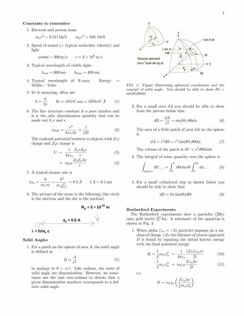
1

Constants to remember

1. Electron and proton mass

mec2 = 0.511 MeV mpc

2 = 938.MeV

2. Speed of sound (∼ typical molecular velocity) andlight

sound ∼ 300 m/s c = 3× 108 m/s

3. Typical wavelength of visible light.

λred ∼ 600 nm λblue ∼ 400 nm

4. Typical wavelength of X-rays. Energy ∼50 kilo−Volts

5. 2π is annoying, often use

~ =h

2π~c = 197eV nm = 1970 eV A (1)

6. The fine structure constant is a pure number andis is the only dimensionless quantity that can bemade out ~, c and e

αEM =e2

4πεo~c' 1

137(2)

The coulomb potential between to objects with Z1echarge and Z2e charge is

U =1

4πεo

Z1eZ2e

r(3)

= αEMZ1Z2 ~c

r(4)

7. A typical atomic size is

1ao =~

mecα=

~2

m e2

4πεo

∼ 0.5 A 1 A = 0.1 nm

8. The picture of the atom is the following (the circleis the electron and the dot is the nucleus)

m-15 10× = 5 AR

ce = h/mλ

= 0.5 A0a

Solid Angles

1. For a patch on the sphere of area A, the solid angleis defined as

Ω ≡ A

r2(5)

in analogy to θ = s/r. Like radians, the units ofsolid angle are dimensionless. However, we some-times use the unit ster-radians to denote that agiven dimensionless numbers corresponds to a def-inite solid angle.

10/19/08 9:14 PMGoogle Image Result for http://hyperphysics.phy-astr.gsu.edu/hbase/math/immath/sphel.gif

Page 1 of 3http://images.google.com/imgres?imgurl=http://hyperphysics.phy-ast…ysics%26um%3D1%26hl%3Den%26client%3Dsafari%26rls%3Den-us%26sa%3DG

Spherical Polar Coordinates

Applications LaPlacian Gradient Divergence Curl

Index

HyperPhysics****HyperMath*****Geometry Go Back

Cylindrical Polar Coordinates

With the axis of the circular cylinder taken as the z-axis, the

perpendicular distance from the cylinder axis is designated by r

and the azimuthal angle taken to be f .

Applications LaPlacian Gradient Divergence Curl

Index

FIG. 1: Figure illustrating spherical coordinates and theconcept of solid angle. You should be able to show dΩ =sin(Θ)dΘdφ

2. For a small area dA you should be able to showfrom the picture below that

dΩ =dA

r2= sin(Θ) dΘdφ (6)

The area of a little patch of area dA on the sphereis

dA = r2dΩ = r2 sin(Θ) dΘdφ (7)

The volume of the patch is dV = r2dΘdφdr

3. The integral of some quantity over the sphere is∫sphere

dΩ . . . =

∫ π

0

dΘ sin Θ

∫ 2π

0

dφ . . . (8)

4. For a small cylindrical stip as shown below youshould be able to show that

dΩ = 2π sin(Θ)dΘ (9)

Rutherford ExperimentsThe Rutherford experiments shot α particles (4

2He)onto gold nuclei 197

79 Au. A schematic of the appartus isshown in Fig. 3

1. When alpha (zα = +2) particles impinge on a nu-cleus of charge +Ze the distance of closest approachD is found by equating the initial kinetic energywith the final potential energy

K =1

2mαv

2α =

1

4πεo

(Ze)(zαe)

D(10)

1

2mαv

2α = αEM

Zzα~cD

(11)

i.e.

D = αEM

(Zzα~c12mαv2

α

)

2

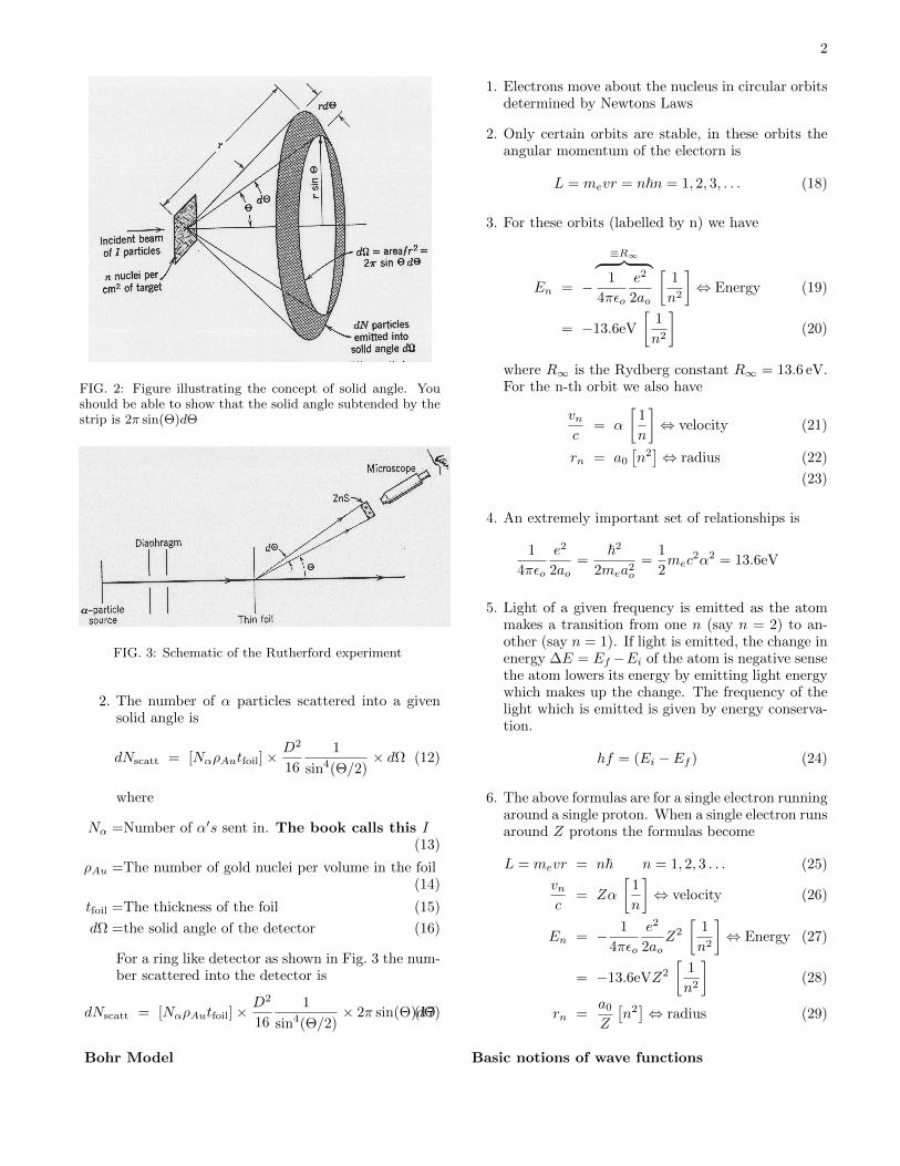
FIG. 2: Figure illustrating the concept of solid angle. Youshould be able to show that the solid angle subtended by thestrip is 2π sin(Θ)dΘ

FIG. 3: Schematic of the Rutherford experiment

2. The number of α particles scattered into a givensolid angle is

dNscatt = [NαρAutfoil]×D2

16

1

sin4(Θ/2)× dΩ (12)

where

Nα =Number of α′s sent in. The book calls this I(13)

ρAu =The number of gold nuclei per volume in the foil(14)

tfoil =The thickness of the foil (15)

dΩ =the solid angle of the detector (16)

For a ring like detector as shown in Fig. 3 the num-ber scattered into the detector is

dNscatt = [NαρAutfoil]×D2

16

1

sin4(Θ/2)× 2π sin(Θ)dΘ(17)

Bohr Model

1. Electrons move about the nucleus in circular orbitsdetermined by Newtons Laws

2. Only certain orbits are stable, in these orbits theangular momentum of the electorn is

L = mevr = n~n = 1, 2, 3, . . . (18)

3. For these orbits (labelled by n) we have

En = −

≡R∞︷ ︸︸ ︷1

4πεo

e2

2ao

[1

n2

]⇔ Energy (19)

= −13.6eV

[1

n2

](20)

where R∞ is the Rydberg constant R∞ = 13.6 eV.For the n-th orbit we also have

vnc

= α

[1

n

]⇔ velocity (21)

rn = a0

[n2]⇔ radius (22)

(23)

4. An extremely important set of relationships is

1

4πεo

e2

2ao=

~2

2mea2o

=1

2mec

2α2 = 13.6eV

5. Light of a given frequency is emitted as the atommakes a transition from one n (say n = 2) to an-other (say n = 1). If light is emitted, the change inenergy ∆E = Ef −Ei of the atom is negative sensethe atom lowers its energy by emitting light energywhich makes up the change. The frequency of thelight which is emitted is given by energy conserva-tion.

hf = (Ei − Ef ) (24)

6. The above formulas are for a single electron runningaround a single proton. When a single electron runsaround Z protons the formulas become

L = mevr = n~ n = 1, 2, 3 . . . (25)

vnc

= Zα

[1

n

]⇔ velocity (26)

En = − 1

4πεo

e2

2aoZ2

[1

n2

]⇔ Energy (27)

= −13.6eVZ2

[1

n2

](28)

rn =a0

Z

[n2]⇔ radius (29)

Basic notions of wave functions

3

1. DeBroglie says that the momentum is related tothe wavelength

p =h

λ= ~

2π

λ= ~k (30)

2. Similarly the frequency determines energy

E = ~ω ω = 2πν (31)

where ν is the frequency.

3. If the typical size of the wave function is ∆x thenthe typical spread is in the momentum ∆p is deter-mined by the uncertainty relation

∆x∆p ∼ ~ (32)

4. Similarly if the typical duration of a wave pulse (ofe.g. sound, E&M, or electron wave) is ∆t then itsfrequency ω is only determined to within 1/∆t. Inquantum mechanics this is written

∆t∆ω ∼ 1 or ∆t∆E >∼ ~

i.e. if something is observed for a short period oftime its energy can not be precisely known

5. In general an attractive potential energy tends tolocalize (make smaller) the particles wave function.As the particle is localized the kinetic energy in-creases. The balance determines the typical extentof the wave function (or the size of the object).

Wave packets

1. A general wave can be written as a sum of sin’sand cos’s. For a general wave then there is not onemomentum and energy associated with the particlebut a range of momenta and energies characterizedby ∆ω and ∆k

2. Consider the addition of two waves

Ψ1(x, t) = sin(k1x− ω1t) Ψ2(x, t) = sin(k2x− ω2t)

The waves have a certain average frequency (en-ergy) ω = (ω1 + ω2)/2 and a frequency spread∆ω = ω2 − ω = (ω2 − ω1)/2. Similarly the twowaves have an average wave number (momentum)k = k1 + k2 and ∆k = (k2− k1)/2. The sum of thetwo waves is

Ψ1 + Ψ2 = 2 sin(kx− ωt)︸ ︷︷ ︸Carrier wave

cos(∆kx−∆ωt)︸ ︷︷ ︸Envelope Wave

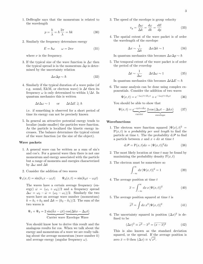
You should know how to derive this result and theanalagous results for cos. When we talk about theenergy and momentum of a wave we are really talk-ing about the average momentum (wave number k)and average energy (angular frequency ω).

3. The speed of the envelope is group velocity

vg =∆ω

∆k=dω

dk=dE

dp(33)

4. The spatial extent of the wave packet is of orderthe wavelength of the envelope

∆x ∼ 1

∆k∆x∆k ∼ 1 (34)

In quantum mechanics this becomes ∆x∆p ∼ ~

5. The temporal extent of the wave packet is of orderthe period of the evnvelop

∆t ∼ 1

∆ω∆t∆ω ∼ 1 (35)

In quantum mechanics this becomes ∆t∆E ∼ ~

6. The same analysis can be done using complex ex-ponentials. Consider the addition of two waves

Ψ(x, t) = e−iω1t+ik1x + e−iω2t+ik2x (36)

You should be able to show that

Ψ(x, t) = e−iωt+ikx︸ ︷︷ ︸carrier

2 cos (∆ωt−∆kx)︸ ︷︷ ︸envelope

(37)

Wavefunctions

1. The electron wave function squared |Ψ(x), t|2 =P(x, t) is a probability per unit length to find theparticle at time t. The the probability dP to finda particle between x and x+ dx at time t

dP = P(x, t)dx = |Ψ(x, t)|2dx (38)

2. The most likely location at time t may be found bymaximizing the probability density P(x, t)

3. The electron must be somewhere so∫ ∞−∞

dx |Ψ(x, t)|2 = 1 (39)

4. The average position at time t

x =

∫ ∞−∞

dxx |Ψ(x, t)|2 (40)

5. The average position squared at time t is

x2 =

∫dxx2 |Ψ(x, t)|2 (41)

6. The uncertainty squared in position (∆x)2 is de-fined to be

(∆x)2 ≡ x2 − x2 = (x− x)2 (42)

This is also known as the standard deviationsquared, or the spread. If the average position is

zero x = 0 then (∆x) ≡√x2.

4

Momentum Averages

1. We use a notation for “Operators”

x =

∫ +∞

−∞dxΨ∗(x)XΨ(x) (43)

=

∫ +∞

−∞dxΨ∗(x)xΨ(x) (44)

Here X is an simply an “operator” which takesthe function Ψ(x) and spits out the new functionxΨ(x). It just gives a notation to things thatwe alaready understand, for example X2Ψ(x) =XxΨ(x) = x2Ψ(x)

2. The average momentum is

p =

∫ +∞

−∞dxΨ∗(x)PΨ(x) (45)

=

∫ +∞

−∞dxΨ∗(x)

(−i~ d

dx

)Ψ(x) (46)

=

∫ +∞

−∞dxΨ∗(x)

(−i~dΨ

dx

)(47)

Here the momentum operator is

P = −i~ d

dx

takes the function Ψ(x) and spits out the derivative−i~dΨ

dx .

3. The average momentum squared is

p2 =

∫ +∞

−∞Ψ∗(x)P2Ψ(x) (48)

=

∫ +∞

−∞Ψ∗(x)

(−~2 d

2

dx2

)Ψ(x) (49)

4. The uncertainty squared in momentum (or stan-dard deviation squared) is defined like for (∆x)2

(∆p)2 ≡ p2 − p2 (50)

Again if p is zero then ∆p ≡√p2 is the “root mean

square” momentum.

5. The average kinetic energy is

KE =

∫ +∞

−∞Ψ∗(x)

[− ~2

2m

d2

dx2

]Ψ(x) (51)

6. The formal statement of the uncertainty principleis

(∆x)(∆p) ≥ ~2

(52)

where the standard deviation in position ∆x andmomentum ∆p are defined as above. (You can seewhy its a good thing that we know how to use itbefore we can state it precisely)

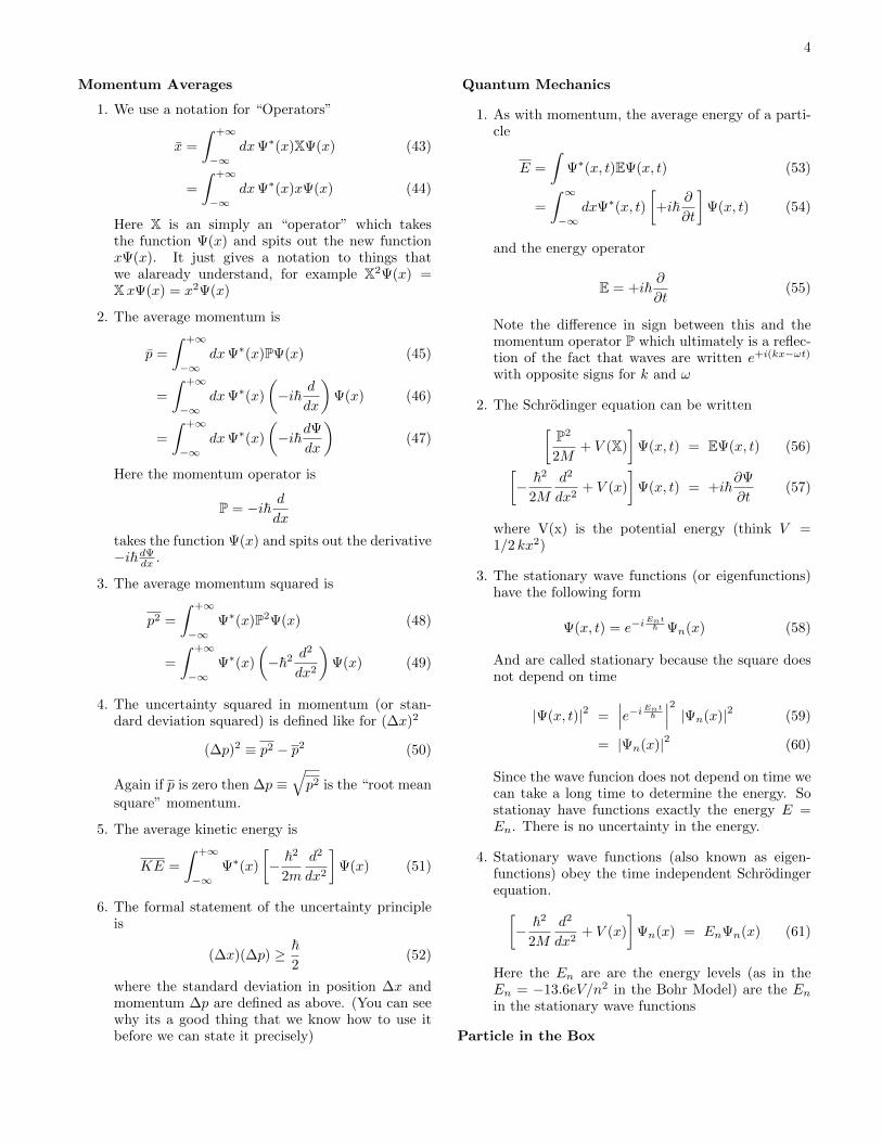
Quantum Mechanics

1. As with momentum, the average energy of a parti-cle

E =

∫Ψ∗(x, t)EΨ(x, t) (53)

=

∫ ∞−∞

dxΨ∗(x, t)

[+i~

∂

∂t

]Ψ(x, t) (54)

and the energy operator

E = +i~∂

∂t(55)

Note the difference in sign between this and themomentum operator P which ultimately is a reflec-tion of the fact that waves are written e+i(kx−ωt)

with opposite signs for k and ω

2. The Schrodinger equation can be written[P2

2M+ V (X)

]Ψ(x, t) = EΨ(x, t) (56)[

− ~2

2M

d2

dx2+ V (x)

]Ψ(x, t) = +i~

∂Ψ

∂t(57)

where V(x) is the potential energy (think V =1/2 kx2)

3. The stationary wave functions (or eigenfunctions)have the following form

Ψ(x, t) = e−iEnt~ Ψn(x) (58)

And are called stationary because the square doesnot depend on time

|Ψ(x, t)|2 =∣∣∣e−iEnt

~

∣∣∣2 |Ψn(x)|2 (59)

= |Ψn(x)|2 (60)

Since the wave funcion does not depend on time wecan take a long time to determine the energy. Sostationay have functions exactly the energy E =En. There is no uncertainty in the energy.

4. Stationary wave functions (also known as eigen-functions) obey the time independent Schrodingerequation.[− ~2

2M

d2

dx2+ V (x)

]Ψn(x) = EnΨn(x) (61)

Here the En are are the energy levels (as in theEn = −13.6eV/n2 in the Bohr Model) are the Enin the stationary wave functions

Particle in the Box

5

1. For an electron bouncing around in a box of size athe stationary wave functions (eigen-functions) are

Ψn(x) =

√

2a cos

(nπxa

)n = 1, 3, 5, . . .√

2a sin

(nπxa

)n = 2, 4, 6, . . .

(62)

while the stationary energies are

En =~2k2

n

2M=

~2π2

2Ma2n2 n = 1, 2, 3, 4, 5, . . . (63)

Harmonic Oscillator

1. For the harmonic oscillator potential V = 1/2k x2.The classical oscillation frequency is

ωo =

√k

M

2. The energies are

En = ~ωo(n+1

2) n = 0, 1, 2, 3 . . .

Note that n starts at zero in this case

3. The wave functions are given in the tables.

Qualitative Features of Schrodinger Equation

[−~2

2m

d2

dx2+ V (x)

]Ψn(x) = EnΨn(x) (64)

1. In the classically allowed region the egein-functionsoscillates. In the classically forbidden region thewave function decays exponentially. For a givenpotential you should be able to roughly sketch thewave functions.

2. In the classically allowed region E > V , you beable to show (by assuming that the potential Vis constant) that the wave function oscillates withwave number k = 2π/λ as

Ψ(k) ∝ A cos(kx)+B sin(kx) where k ∼√

2m(E − V )

~2

(65)

3. In the classically forbidden region E < V , we saythat the particle is “under the barrier” because E <V . Assuming that the potential is constant youshould be able to show wave function decreases as

Ψ ∼ Ce−κx where κ ∼√

2m(V − E)

~2, (66)

as one goes deeper into the classically forbiddenregion. The length D ≡ 1/(2κ) is known as the“penetration” depth. It is the length over whichthe probability decreases by a factor 1/e.

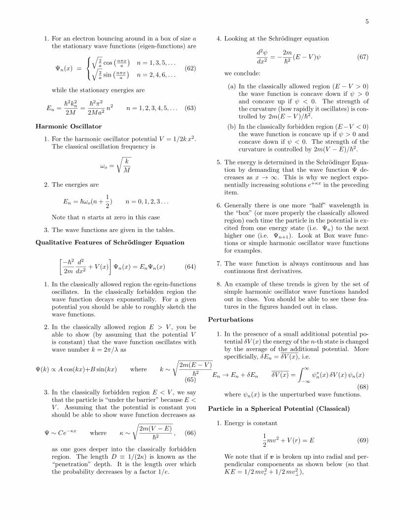
4. Looking at the Schrodinger equation

d2ψ

dx2= −2m

~2(E − V )ψ (67)

we conclude:

(a) In the classically allowed region (E − V > 0)the wave function is concave down if ψ > 0and concave up if ψ < 0. The strength ofthe curvature (how rapidly it oscillates) is con-trolled by 2m(E − V )/~2.

(b) In the classically forbidden region (E−V < 0)the wave function is concave up if ψ > 0 andconcave down if ψ < 0. The strength of thecurvature is controlled by 2m(V − E)/~2.

5. The energy is determined in the Schrodinger Equa-tion by demanding that the wave function Ψ de-creases as x → ∞. This is why we neglect expo-nentially increasing solutions e+κx in the precedingitem.

6. Generally there is one more “half” wavelength inthe “box” (or more properly the classically allowedregion) each time the particle in the potential is ex-cited from one energy state (i.e. Ψn) to the nexthigher one (i.e. Ψn+1). Look at Box wave func-tions or simple harmonic oscillator wave functionsfor examples.

7. The wave function is always continuous and hascontinuous first derivatives.

8. An example of these trends is given by the set ofsimple harmonic oscillator wave functions handedout in class. You should be able to see these fea-tures in the figures handed out in class.

Perturbations

1. In the presence of a small additional potential po-tential δV (x) the energy of the n-th state is changedby the average of the additional potential. Morespecificially, δEn = δV (x), i.e.

En → En + δEn δV (x) =

∫ ∞−∞

ψ∗n(x) δV (x)ψn(x)

(68)where ψn(x) is the unperturbed wave functions.

Particle in a Spherical Potential (Classical)

1. Energy is constant

1

2mv2 + V (r) = E (69)

We note that if v is broken up into radial and per-pendicular compoenents as shown below (so thatKE = 1/2mv2

r + 1/2mv2⊥),

6

!r!v

v!vr

we use that 1/2mv2⊥ = L2/(2mr2) yeilding

1

2mv2

r +L2

2mr2+ V (r)︸ ︷︷ ︸

≡Veff (r)

= E (70)

where we have defined the effective potential

Veff(r) = V (r) +L2

2mr2(71)

(a) E − V determines the kinetic energy

(b) E − Veff(r) determines the radial KE or1/2mv2

r

(c) Veff depends on the angular momentum of theorbit

2. The angular momentum is a constant. This is be-cause the force points along r and hence the torqueτ = r × F = 0. Thus for a classical orbit

L = mrv⊥ = mr2ω (72)

is constant. You should also remember that v⊥ canbe related to the angular velocity

v⊥ = rω where ω =dθ

dt

For small radii ω is large, while for large radii ω issmall

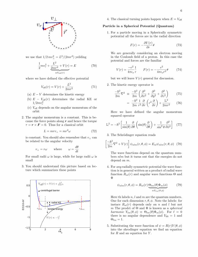
3. You should understand this picture based on lec-ture which summarizes these points

0 2 4 6 8−1.5

−1

−0.5

0

0.5

E/1

3.6

eV

r/ao

kinetic energy

radial KE

centrifugal barrier

rmin rmax

V (r) ∝ − e2

r

Veff(r) = V (r) + L2

2mr2

4. The classical turning points happen when E = Veff

Particle in a Spherical Potential (Quantum)

1. For a particle moving in a Spherically symmetricpotiential all the forces are in the radial direction

F (r) = −∂V (r)

∂rr (73)

We are generally considering an electron movingin the Coulomb field of a proton. In this case thepotential and forces are the familiar

V (r) =−e2

4πεo

1

rF (r) = − e2

4πεor2r (74)

but we will leave V (r) general for discussion.

2. The kinetic energy operator is

−~2

2m∇2 ≡ −~

2

2m

(∂2

∂x2+

∂2

∂y2+

∂2

∂z2

)(75)

=−~2

2m

1

r2

∂

∂r

(r2 ∂

∂r

)+

L2

2mr2(76)

Here we have defined the angular momentumsquared operator

L2 = −~2

[1

sin(θ)

∂

∂θ

(sin(θ)

∂

∂θ

)+

1

sin2 θ

∂2

∂φ2

](77)

3. The Schrodinger equation reads[−~2

2m∇2 + V (r)

]ψnlm(r, θ, φ) = Enlψnlm(r, θ, φ) (78)

The wave functions depend on the quantum num-bers nlm but it turns out that the energies do notdepend on m.

4. For any radially symmetric potential the wave func-tion is in general written as a product of radial wavefunction Rnl(r) and angular wave functions Θ andΦ

ψnlm(r, θ, φ) = Rnl(r) Θlm(θ)Φm(φ)︸ ︷︷ ︸≡Ylm(θ,φ)

(79)

Here th labels n, l and m are the quantum numbers.One for each dimension r, θ, φ. Note the labels: forinstace Rnl(r) depends only on n and l but notm The prodct of Θ and Φ is known as a sphericalharmonic Ylm(θ, φ) ≡ Θlm(θ)Φm(φ). For ` = 0there is no angular dependence and Y00 = 1 andΘlm = 1.

5. Substituting the wave function of ψ = R(r)Y (θ, φ)into the shrodinger equation we find an equationfor R and an equation for Y .

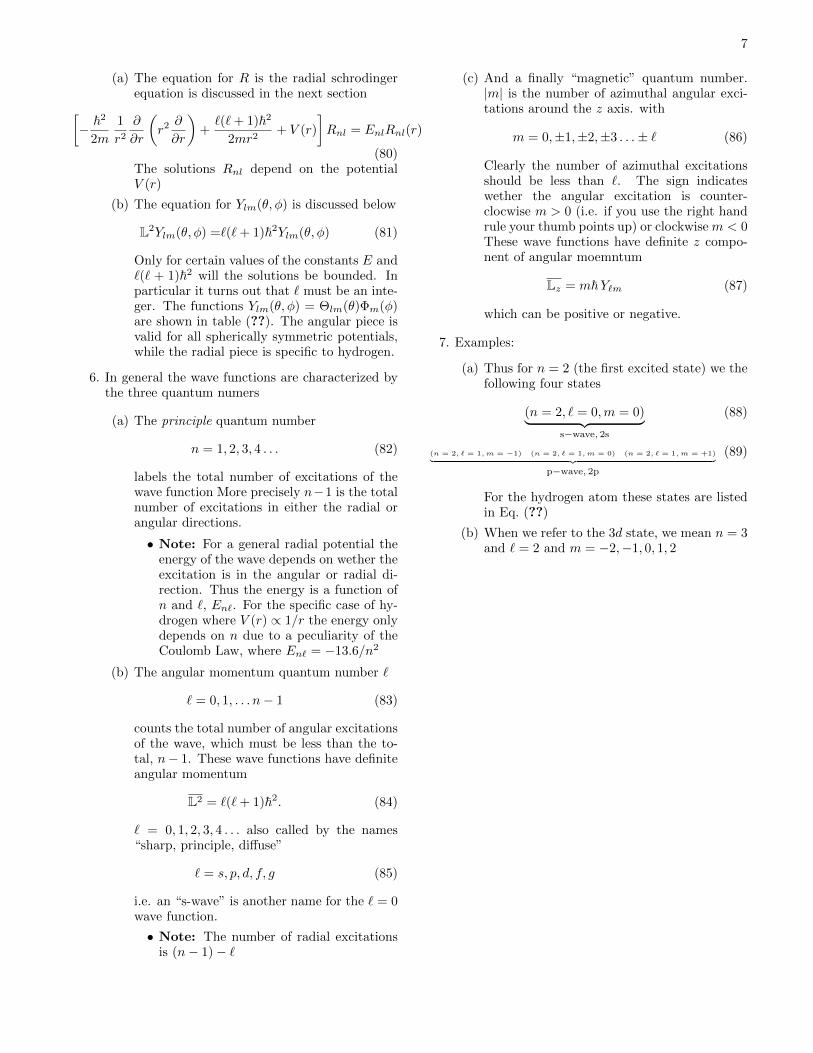
7

(a) The equation for R is the radial schrodingerequation is discussed in the next section[

− ~2

2m

1

r2

∂

∂r

(r2 ∂

∂r

)+`(`+ 1)~2

2mr2+ V (r)

]Rnl = EnlRnl(r)

(80)The solutions Rnl depend on the potentialV (r)

(b) The equation for Ylm(θ, φ) is discussed below

L2Ylm(θ, φ) =`(`+ 1)~2Ylm(θ, φ) (81)

Only for certain values of the constants E and`(` + 1)~2 will the solutions be bounded. Inparticular it turns out that ` must be an inte-ger. The functions Ylm(θ, φ) = Θlm(θ)Φm(φ)are shown in table (??). The angular piece isvalid for all spherically symmetric potentials,while the radial piece is specific to hydrogen.

6. In general the wave functions are characterized bythe three quantum numers

(a) The principle quantum number

n = 1, 2, 3, 4 . . . (82)

labels the total number of excitations of thewave function More precisely n−1 is the totalnumber of excitations in either the radial orangular directions.

• Note: For a general radial potential theenergy of the wave depends on wether theexcitation is in the angular or radial di-rection. Thus the energy is a function ofn and `, En`. For the specific case of hy-drogen where V (r) ∝ 1/r the energy onlydepends on n due to a peculiarity of theCoulomb Law, where En` = −13.6/n2

(b) The angular momentum quantum number `

` = 0, 1, . . . n− 1 (83)

counts the total number of angular excitationsof the wave, which must be less than the to-tal, n− 1. These wave functions have definiteangular momentum

L2 = `(`+ 1)~2. (84)

` = 0, 1, 2, 3, 4 . . . also called by the names“sharp, principle, diffuse”

` = s, p, d, f, g (85)

i.e. an “s-wave” is another name for the ` = 0wave function.

• Note: The number of radial excitationsis (n− 1)− `

(c) And a finally “magnetic” quantum number.|m| is the number of azimuthal angular exci-tations around the z axis. with

m = 0,±1,±2,±3 . . .± ` (86)

Clearly the number of azimuthal excitationsshould be less than `. The sign indicateswether the angular excitation is counter-clocwise m > 0 (i.e. if you use the right handrule your thumb points up) or clockwise m < 0These wave functions have definite z compo-nent of angular moemntum

Lz = m~Y`m (87)

which can be positive or negative.

7. Examples:

(a) Thus for n = 2 (the first excited state) we thefollowing four states

(n = 2, ` = 0,m = 0)︸ ︷︷ ︸s−wave, 2s

(88)

(n = 2, ` = 1,m = −1) (n = 2, ` = 1,m = 0) (n = 2, ` = 1,m = +1)︸ ︷︷ ︸p−wave, 2p

(89)

For the hydrogen atom these states are listedin Eq. (??)

(b) When we refer to the 3d state, we mean n = 3and ` = 2 and m = −2,−1, 0, 1, 2

8

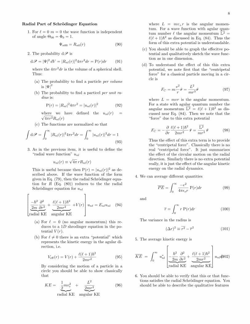
Radial Part of Schrodinger Equation

1. For ` = 0 m = 0 the wave function is independentof angle Θ00 = Φ0 = 1.

Ψn00 = Rn0(r) (90)

2. The probability dP is

dP = |Ψ|2 dV = |Rnl(r)|24πr2dr = P(r)dr (91)

where the 4πr2dr is the volume of a spherical shell.Thus:

(a) The probability to find a particle per volume

is |Ψ|2

(b) The probability to find a particel per unit ra-dius is:

P(r) = |Rnl|24πr2 = |unl(r)|2 (92)

where we have defined the unl(r) =√4πr2Rnl(r)

(c) The functions are normalized so that∫dP =

∫ ∞0

|Rnl(r)|24πr2dr =

∫ ∞0

|unl(r)|2dr = 1

(93)

3. As in the previous item, it is useful to define the“radial wave function” unl

unl(r) ≡√

4π rRnl(r)

This is useful because then P(r) = |unl(r)|2 as de-scribed above. If the wave function of the formgiven in Eq. (79), then the radial Schrodinger equa-tion for R (Eq. (80)) reduces to the the radialSchrodinger equation for unl −~2

2m

∂2

∂r2︸ ︷︷ ︸radial KE

+`(`+ 1)~2

2mr2︸ ︷︷ ︸angular KE

+V (r)

un` = Enlunl (94)

(a) For ` = 0 (no angular momentum) this re-duces to a 1D shrodinger equation in the po-tential V (r).

(b) For ` 6= 0 there is an extra “potential” whichrepresents the kinetic energy in the agular di-rection, i.e.

Veff(r) = V (r) +`(`+ 1)~2

2mr2(95)

By considering the motion of a particle in acircle you should be able to show classicallythat

KE =1

2mv2

r︸ ︷︷ ︸radial KE

+L2

2mr2︸ ︷︷ ︸angular KE

(96)

where L = mv⊥r is the angular momen-tum. For a wave function with agular quan-tum number ` the angular momentum L2 =`(` + 1)~2 as discussed in Eq. (84). Thus theform of this extra potential is understandable.

(c) You should be able to graph the effecitve po-tential and qualitatively sketch the wave func-tion as in one dimension.

(d) To understand the effect of this this extrapotential, we note first that the “centripetalforce” for a classical particle moving in a cir-cle is

FC = mv2

rr =

L2

mr3r (97)

where L = mvr is the angular momentum.For a state with agular quantum number theangular momentum L2 = `(` + 1)~2 as dis-cussed near Eq. (84). Then we note that the“force” due to this extra potential

FC = − ∂

∂r

`(`+ 1)~2

2mr2r =

L2

mr3r (98)

Thus the effect of this extra term is to providethe “centripetal force”. Classically there is noreal “centripetal force”. It just summarizesthe effect of the circular motion on the radialdirection. Similarly there is no extra potentialreally, it is just the effect of the angular kineticenergy on the radial dynamics.

4. We can average different quantities

PE =

∫ ∞0

−e2

4πεorP(r)dr (99)

and

r =

∫ ∞0

r P(r)dr (100)

The variance in the radius is

(∆r)2 ≡ r2 − r2 (101)

5. The average kinetic energy is

KE =

∫ ∞0

u∗nl

− ~2

2m

∂2

∂r2︸ ︷︷ ︸radial KE

+`(`+ 1)~2

2mr2︸ ︷︷ ︸angular KE

unldr(102)

6. You should be able to verify that this or that func-tions satisfies the radial Schrodinger equation. Youshould be able to describe the qualitative features

9

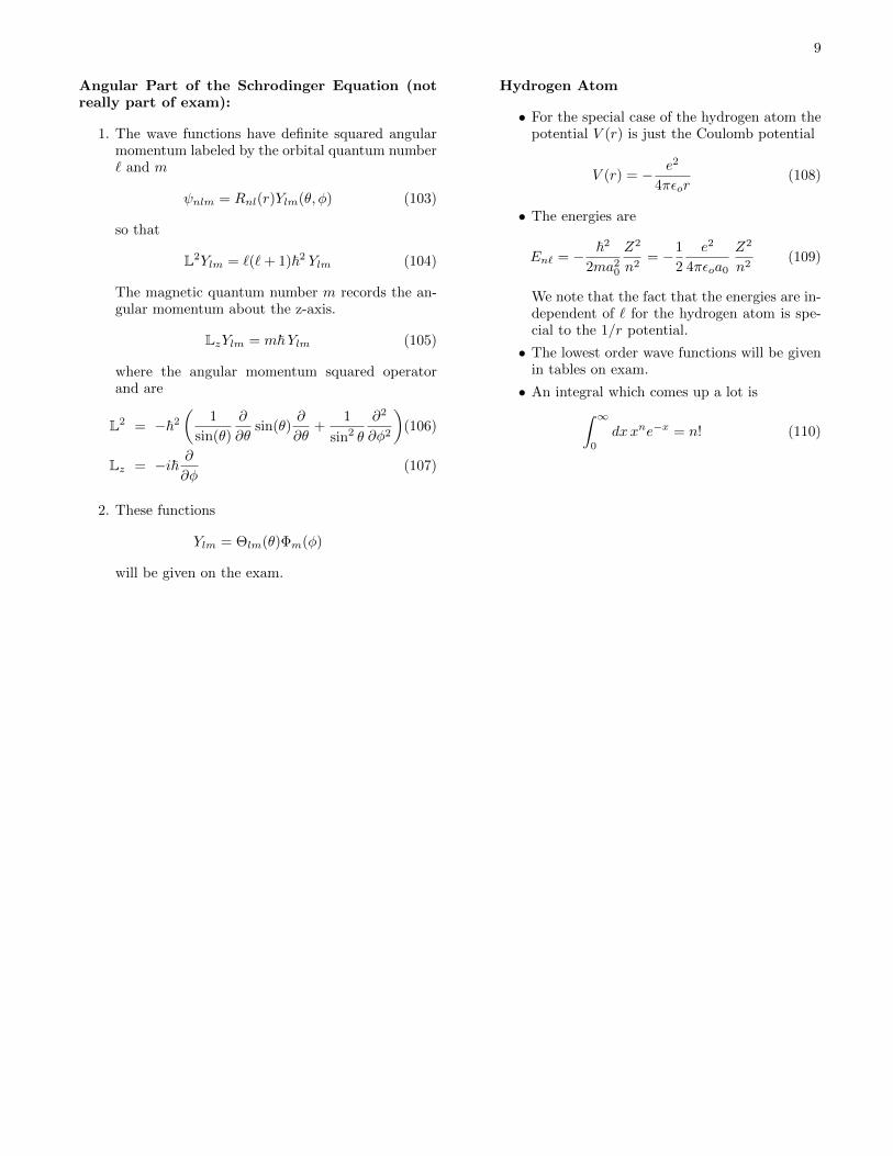
Angular Part of the Schrodinger Equation (notreally part of exam):

1. The wave functions have definite squared angularmomentum labeled by the orbital quantum number` and m

ψnlm = Rnl(r)Ylm(θ, φ) (103)

so that

L2Ylm = `(`+ 1)~2 Ylm (104)

The magnetic quantum number m records the an-gular momentum about the z-axis.

LzYlm = m~Ylm (105)

where the angular momentum squared operatorand are

L2 = −~2

(1

sin(θ)

∂

∂θsin(θ)

∂

∂θ+

1

sin2 θ

∂2

∂φ2

)(106)

Lz = −i~ ∂

∂φ(107)

2. These functions

Ylm = Θlm(θ)Φm(φ)

will be given on the exam.

Hydrogen Atom

• For the special case of the hydrogen atom thepotential V (r) is just the Coulomb potential

V (r) = − e2

4πεor(108)

• The energies are

En` = − ~2

2ma20

Z2

n2= −1

2

e2

4πεoa0

Z2

n2(109)

We note that the fact that the energies are in-dependent of ` for the hydrogen atom is spe-cial to the 1/r potential.

• The lowest order wave functions will be givenin tables on exam.

• An integral which comes up a lot is∫ ∞0

dxxne−x = n! (110)

10

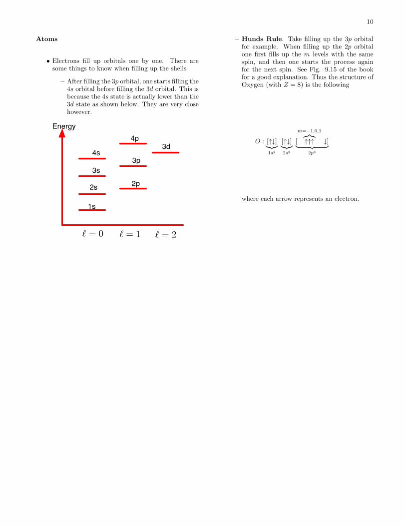
Atoms

• Electrons fill up orbitals one by one. There aresome things to know when filling up the shells

– After filling the 3p orbital, one starts filling the4s orbital before filling the 3d orbital. This isbecause the 4s state is actually lower than the3d state as shown below. They are very closehowever.

1s

2s 2p3s

3p4s

3d4p

Energy

! = 0 ! = 1 ! = 2

– Hunds Rule. Take filling up the 3p orbitalfor example. When filling up the 2p orbitalone first fills up the m levels with the samespin, and then one starts the process againfor the next spin. See Fig. 9.15 of the bookfor a good explanation. Thus the structure ofOxygen (with Z = 8) is the following

O : [↑↓]︸︷︷︸1s2

[↑↓]︸︷︷︸2s2

[

m=−1,0,1︷︸︸︷↑↑↑ ↓]︸ ︷︷ ︸

2p4

where each arrow represents an electron.