Spherical f-Tilings by Scalene Triangles

and Isosceles Trapezoids IIICatarina P. Avelino ∗ Altino F. Santos †

Department of MathematicsUTAD, 5001 - 801 Vila Real, Portugal

Submitted: Jun 23, 2009; Accepted: Jul 13, 2009; Published: Jul 24, 2009

Mathematics Subject Classification: 52C20, 52B05, 20B35

Abstract

The study of the dihedral f-tilings of the sphere S2 whose prototiles are a sca-lene triangle and an isosceles trapezoid was initiated in [7, 8]. In this paper wecomplete this classification presenting the study of all dihedral spherical f-tilingsby scalene triangles and isosceles trapezoids in the remaining case of adjacency. Alist containing all the f-tilings obtained in this paper is presented in Table 1. It iscomposed by isolated tilings as well as discrete and continuous families of tilings.The combinatorial structure is also achieved.

Keywords: dihedral f-tilings, combinatorial properties, spherical trigonometry

1 Introduction

Let S2 be the Euclidean sphere of radius 1. By a dihedral folding tiling (f-tiling , for short)of the sphere S2 whose prototiles are a spherical isosceles trapezoid, Q, and a sphericaltriangle, T , we mean a polygonal subdivision τ of S2 such that each cell (tile) of τ iscongruent to Q or T and the vertices of τ satisfy the angle-folding relation, i.e., eachvertex of τ is of even valency 2n, n ≥ 2, and the sums of alternate angles are equal; thatis,

n∑

i=1

θ2i =

n∑

i=1

θ2i−1 = π,

where the angles θi around any vertex of τ are ordered cyclically.

∗(cavelino@utad.pt)†(afolgado@utad.pt)

Supported partially by the Research Unit CM–UTAD of University of Tras-os-Montes e Alto Douro,through the Foundation for Science and Technology (FCT).

the electronic journal of combinatorics 16 (2009), #R87 1

Folding tilings are intrinsically related to the theory of isometric foldings on Rie-mannian manifolds. In fact, the set of singularities of any spherical isometric foldingcorresponds to a folding tiling of the sphere, see [9] for the foundations of this subject.

The study of dihedral f-tilings of the sphere started in 2004 [1, 2, 3], where the clas-sification of all dihedral f-tilings by spherical parallelograms and spherical triangles wasobtained. Later on, in [5], the classification of all dihedral f-tilings of the sphere by tri-angles and r-sided regular polygons (r ≥ 5) was achieved. In a subsequent paper [4], ispresented the study of all dihedral spherical f-tilings whose prototiles are an equilateraltriangle and an isosceles triangle. Robert Dawson and B. Doyle have also been interestedin special classes of spherical tilings, see [10, 11] for instance.

In this paper we shall discuss dihedral f-tilings by spherical scalene triangles, T , andspherical isosceles trapezoids, Q, with a certain adjacency pattern. We present in Table 1a list containing all the f-tilings obtained in this paper. We shall denote by Ω (Q, T ) theset, up to an isomorphism, of all dihedral f-tilings of S2 whose prototiles are Q and T .

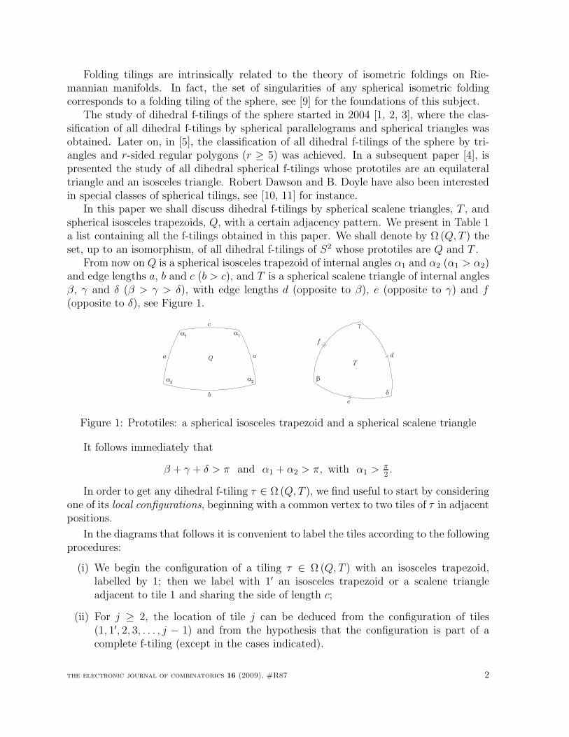
From now on Q is a spherical isosceles trapezoid of internal angles α1 and α2 (α1 > α2)and edge lengths a, b and c (b > c), and T is a spherical scalene triangle of internal anglesβ, γ and δ (β > γ > δ), with edge lengths d (opposite to β), e (opposite to γ) and f

(opposite to δ), see Figure 1.

T

g

d

b

d

f

e

a2a

2

a1

a1

aa

b

c

Q

Figure 1: Prototiles: a spherical isosceles trapezoid and a spherical scalene triangle

It follows immediately that

β + γ + δ > π and α1 + α2 > π, with α1 > π2.

In order to get any dihedral f-tiling τ ∈ Ω (Q, T ), we find useful to start by consideringone of its local configurations, beginning with a common vertex to two tiles of τ in adjacentpositions.

In the diagrams that follows it is convenient to label the tiles according to the followingprocedures:

(i) We begin the configuration of a tiling τ ∈ Ω (Q, T ) with an isosceles trapezoid,labelled by 1; then we label with 1′ an isosceles trapezoid or a scalene triangleadjacent to tile 1 and sharing the side of length c;

(ii) For j ≥ 2, the location of tile j can be deduced from the configuration of tiles(1, 1′, 2, 3, . . . , j − 1) and from the hypothesis that the configuration is part of acomplete f-tiling (except in the cases indicated).

the electronic journal of combinatorics 16 (2009), #R87 2

2 Dihedral Spherical f-Tilings by Scalene Triangles

and Isosceles Trapezoids

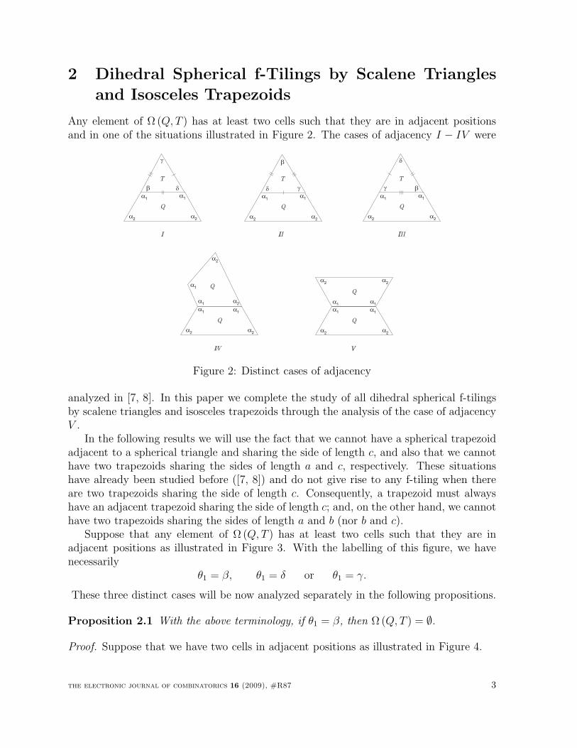
Any element of Ω (Q, T ) has at least two cells such that they are in adjacent positionsand in one of the situations illustrated in Figure 2. The cases of adjacency I − IV were

Q

T

I

b

a1

a1

a2

a2

Q

a1

a1

a2

a2

Q

a1

a1

a2

a2

II

IV

Q

a1

a1

a2

a2

Qa1

a1

a2

a2

V

g

Q

T

b

a1

a1

a2

a2

g

III

Q

T

b

a1

a1

a2

a2

gdd

d

Figure 2: Distinct cases of adjacency

analyzed in [7, 8]. In this paper we complete the study of all dihedral spherical f-tilingsby scalene triangles and isosceles trapezoids through the analysis of the case of adjacencyV .

In the following results we will use the fact that we cannot have a spherical trapezoidadjacent to a spherical triangle and sharing the side of length c, and also that we cannothave two trapezoids sharing the sides of length a and c, respectively. These situationshave already been studied before ([7, 8]) and do not give rise to any f-tiling when thereare two trapezoids sharing the side of length c. Consequently, a trapezoid must alwayshave an adjacent trapezoid sharing the side of length c; and, on the other hand, we cannothave two trapezoids sharing the sides of length a and b (nor b and c).

Suppose that any element of Ω (Q, T ) has at least two cells such that they are inadjacent positions as illustrated in Figure 3. With the labelling of this figure, we havenecessarily

θ1 = β, θ1 = δ or θ1 = γ.

These three distinct cases will be now analyzed separately in the following propositions.

Proposition 2.1 With the above terminology, if θ1 = β, then Ω (Q, T ) = ∅.

Proof. Suppose that we have two cells in adjacent positions as illustrated in Figure 4.

the electronic journal of combinatorics 16 (2009), #R87 3

1

1’

a1

a1

a2

a2

a1

a1

a2

a2

q1

Figure 3: Local configuration

2

1

1’

a1

a1

a2

a2

a1

a1

a2

a2

q2q1b

Figure 4: Local configuration

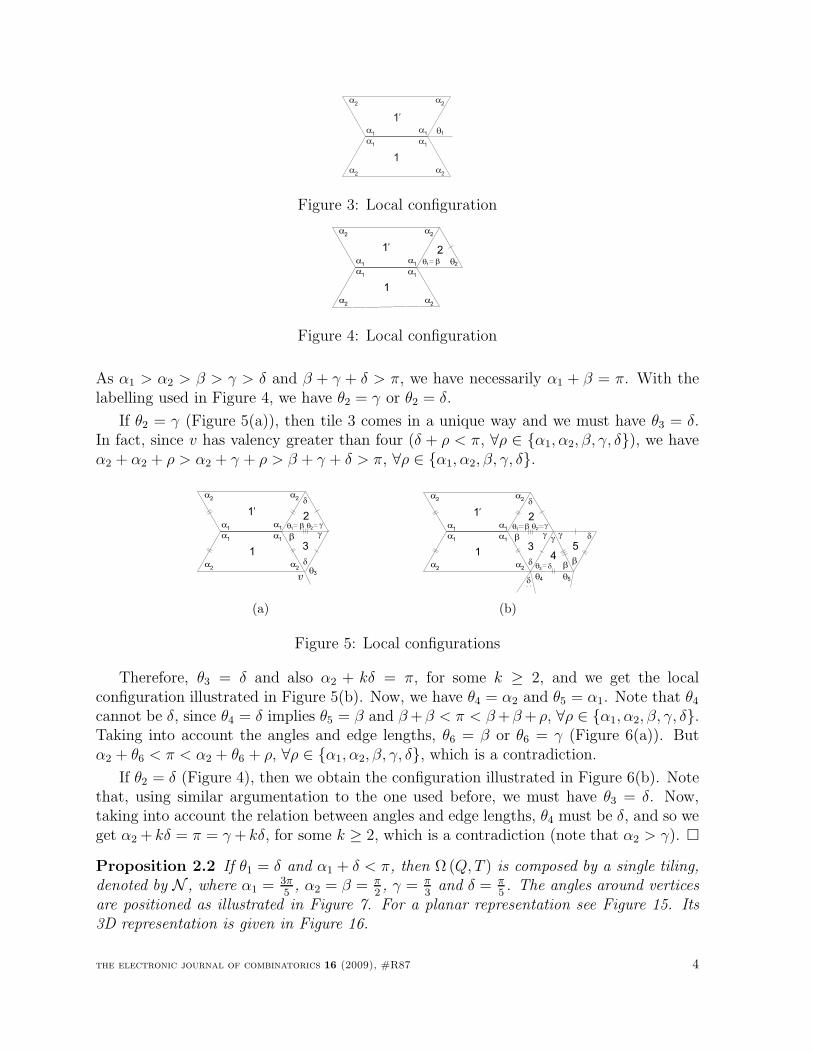
As α1 > α2 > β > γ > δ and β + γ + δ > π, we have necessarily α1 + β = π. With thelabelling used in Figure 4, we have θ2 = γ or θ2 = δ.

If θ2 = γ (Figure 5(a)), then tile 3 comes in a unique way and we must have θ3 = δ.In fact, since v has valency greater than four (δ + ρ < π, ∀ρ ∈ α1, α2, β, γ, δ), we haveα2 + α2 + ρ > α2 + γ + ρ > β + γ + δ > π, ∀ρ ∈ α1, α2, β, γ, δ.

2

3

b

1

1’

q

a1

a1

a2

a2

a1

a1

a2

a2

3

g

g

d

q2

d

q1b

v

(a)

2

3

b

1

1’

a1

a1

a2

a2

a1

a1

a2

a2

g

d

dq

3d

g

b4

g

b

d

5

q4 q5

gq2q1b

d

(b)

Figure 5: Local configurations

Therefore, θ3 = δ and also α2 + kδ = π, for some k ≥ 2, and we get the localconfiguration illustrated in Figure 5(b). Now, we have θ4 = α2 and θ5 = α1. Note that θ4

cannot be δ, since θ4 = δ implies θ5 = β and β +β < π < β +β +ρ, ∀ρ ∈ α1, α2, β, γ, δ.Taking into account the angles and edge lengths, θ6 = β or θ6 = γ (Figure 6(a)). Butα2 + θ6 < π < α2 + θ6 + ρ, ∀ρ ∈ α1, α2, β, γ, δ, which is a contradiction.

If θ2 = δ (Figure 4), then we obtain the configuration illustrated in Figure 6(b). Notethat, using similar argumentation to the one used before, we must have θ3 = δ. Now,taking into account the relation between angles and edge lengths, θ4 must be δ, and so weget α2 + kδ = π = γ + kδ, for some k ≥ 2, which is a contradiction (note that α2 > γ).

Proposition 2.2 If θ1 = δ and α1 + δ < π, then Ω (Q, T ) is composed by a single tiling,denoted by N , where α1 = 3π

5, α2 = β = π

2, γ = π

3and δ = π

5. The angles around vertices

are positioned as illustrated in Figure 7. For a planar representation see Figure 15. Its3D representation is given in Figure 16.

the electronic journal of combinatorics 16 (2009), #R87 4

2

3

b

1

1’

a1

a1

a2

a2

a1

a1

a2

a2

g

d

dq

3d

g

b4

g

b

d

5

dq

4a

2

a1

a2

67

q6

d

gq2q1b

q5

a1

(a)

2

3

b

1

1’

a1

a1

a2

a2

a1

a1

a2

a2 g

g

d

q3

d

g

b4

d

5

q4

b g

dq2q1b

(b)

Figure 6: Local configurations

ddb b

bdd

dd

b b b

a2

a2

dd

a1

a1

dd

gg

g

g

g g

dd

dd

Figure 7: Distinct classes of congruent vertices

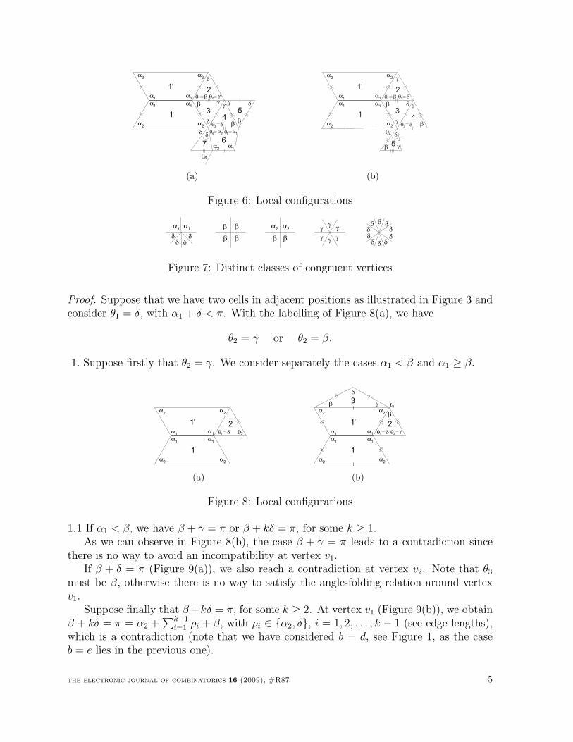
Proof. Suppose that we have two cells in adjacent positions as illustrated in Figure 3 andconsider θ1 = δ, with α1 + δ < π. With the labelling of Figure 8(a), we have

θ2 = γ or θ2 = β.

1. Suppose firstly that θ2 = γ. We consider separately the cases α1 < β and α1 ≥ β.

2

1

1’

a1

a1

a2

a2

a1

a1

a2

a2

q2q1d

(a)

2

1

1’

a1

a1

a2

a2

a1

a1

a2

a2

q1d q2

g

b

gb

d

3 v1

(b)

Figure 8: Local configurations

1.1 If α1 < β, we have β + γ = π or β + kδ = π, for some k ≥ 1.As we can observe in Figure 8(b), the case β + γ = π leads to a contradiction since

there is no way to avoid an incompatibility at vertex v1.If β + δ = π (Figure 9(a)), we also reach a contradiction at vertex v2. Note that θ3

must be β, otherwise there is no way to satisfy the angle-folding relation around vertexv1.

Suppose finally that β +kδ = π, for some k ≥ 2. At vertex v1 (Figure 9(b)), we obtainβ + kδ = π = α2 +

∑k−1i=1 ρi + β, with ρi ∈ α2, δ, i = 1, 2, . . . , k − 1 (see edge lengths),

which is a contradiction (note that we have considered b = d, see Figure 1, as the caseb = e lies in the previous one).

the electronic journal of combinatorics 16 (2009), #R87 5

2

1

1’

a1

a1

a2

a2

a1

a1

a2

a2

q1d q2

g

b

g

b d3

4

d

g b

v1

v2

q3

(a)

2

1

1’

a1

a1

a2

a2

a1

a1

a2

a2

q1d q2

g

b

d

d

v1

(b)

Figure 9: Local configurations

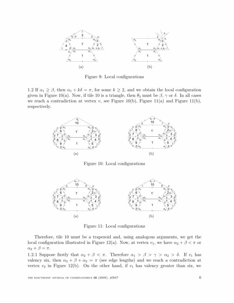
1.2 If α1 ≥ β, then α1 + kδ = π, for some k ≥ 2, and we obtain the local configurationgiven in Figure 10(a). Now, if tile 10 is a triangle, then θ3 must be β, γ or δ. In all caseswe reach a contradiction at vertex v, see Figure 10(b), Figure 11(a) and Figure 11(b),respectively.

2

1

1’

a1

a1

a2

a2

a1

a1

a2

a2

g

3

4

5

q3

6g

g

gg

7

8

9

g

g

dd

d

ddd

d

b

b

b

b

b

b

b

b

q1

dq2

g

10

(a)

2

1

1’

a1

a1

a2

a2

a1

a1

a2

a2

g

3

4

5

6g

g

gg

7

8

9

g

g

dd

d

ddd

d

b

b

b

b

b

b

b

b

q1

dq2

g

10 gd v

q3b

(b)

Figure 10: Local configurations

2

1

1’

a1

a1

a2

a2

a1

a1

a2

a2

g

3

4

5

6g

g

gg

7

8

9

g

g

dd

d

ddd

d

b

b

b

b

b

b

b

b

q1

dq2

g

10 bd v

q3g

(a)

2

1

1’

a1

a1

a2

a2

a1

a1

a2

a2

g

3

4

5

6g

g

gg

7

8

9

g

g

dd

d

ddd

d

b

b

b

b

b

b

b

b

q1

dq2

g

10 bg v

q3 d

(b)

Figure 11: Local configurations

Therefore, tile 10 must be a trapezoid and, using analogous arguments, we get thelocal configuration illustrated in Figure 12(a). Now, at vertex v1, we have α2 + β < π orα2 + β = π.

1.2.1 Suppose firstly that α2 + β < π. Therefore α1 > β > γ > α2 > δ. If v1 hasvalency six, then α2 + β + α2 = π (see edge lengths) and we reach a contradiction atvertex v2 in Figure 12(b). On the other hand, if v1 has valency greater than six, we

the electronic journal of combinatorics 16 (2009), #R87 6

2

1

1’

a1

a1

a2

a2

a1

a1

a2

a2

g

3

4

5

6g

g

gg

7

8

9

g

g

dd

d

ddd

d

b

b

b

b

b

b

b

b

q1

dq2

g

a1

a1

a2

a2

10

a1

a1

a2

a2

11

12

a1

a1

a2

a2

d

d

d

d

v1

(a)

2

1

1’

a1

a1

a2

a2

a1

a1

a2

a2

g

3

4

5

6g

g

gg

7

8

9

g

g

dd

d

ddd

d

b

b

b

b

b

b

b

b

q1

dq2

g

a1

a1

a2

a2

10

a1

a1

a2

a2

11

12

a1

a1

a2

a2

16

g

15

14

13

g

g

dd

d

b

b

b

b

g

d

a1

17

18a

1a

2

a2

a1

a1

a2

a2

a1

a1

v2

(b)

Figure 12: Local configurations

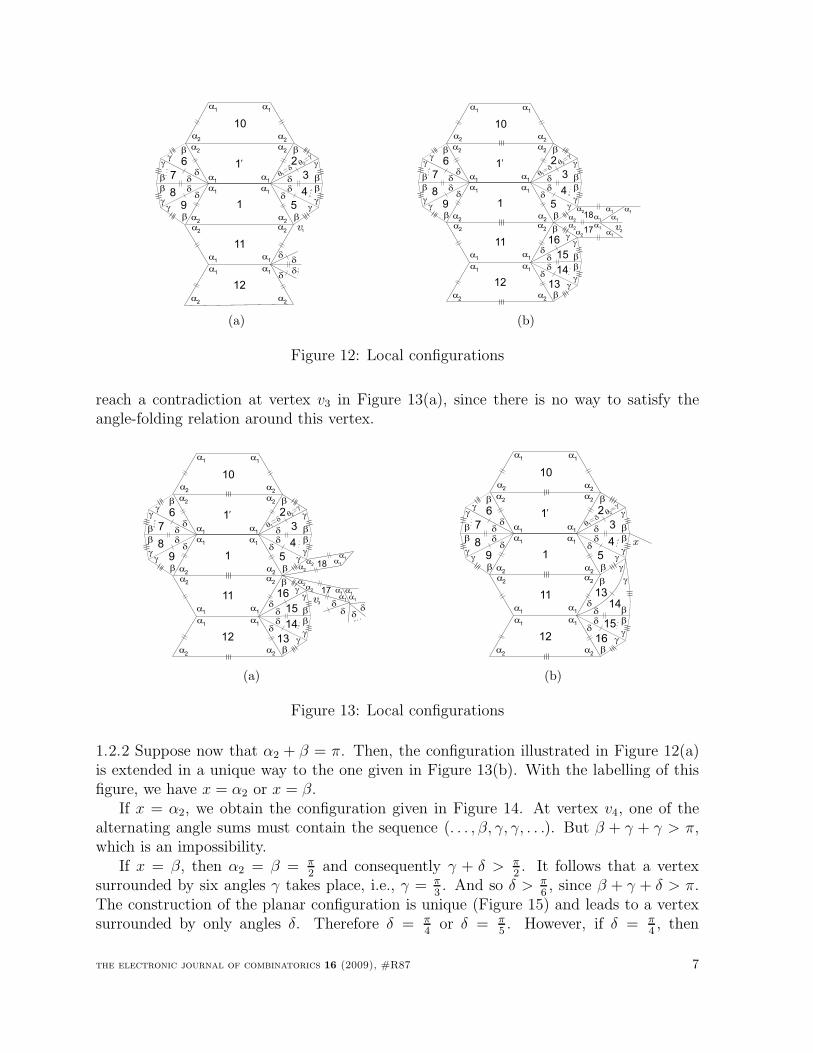
reach a contradiction at vertex v3 in Figure 13(a), since there is no way to satisfy theangle-folding relation around this vertex.

2

1

1’

a1

a1

a2

a2

a1

a1

a2

a2

g

3

4

5

6g

g

gg

7

8

9

g

g

dd

d

ddd

d

b

b

b

b

b

b

b

b

q1

dq2

g

a1

a1

a2

a2

10

a1

a1

a2

a2

11

12

a1

a1

a2

a2

16

g

15

14

13

g

g

dd

d

b

b

b

b

g

d

17

18a

1a

2a2

a1

a1

a2a

2

a1

d

a1

a1

d dd

v3

(a)

2

1

1’

a1

a1

a2

a2

a1

a1

a2

a2

g

3

4

5

6g

g

gg

7

8

9

g

g

dd

d

ddd

d

b

b

b

b

b

b

b

b

q1

dq2

g

a1

a1

a2

a2

10

a1

a1

a2

a2

11

12

a1

a1

a2

a2

13

g

14

15

16

g

g

dd

d

b

b

b

b

g

d

x

(b)

Figure 13: Local configurations

1.2.2 Suppose now that α2 + β = π. Then, the configuration illustrated in Figure 12(a)is extended in a unique way to the one given in Figure 13(b). With the labelling of thisfigure, we have x = α2 or x = β.

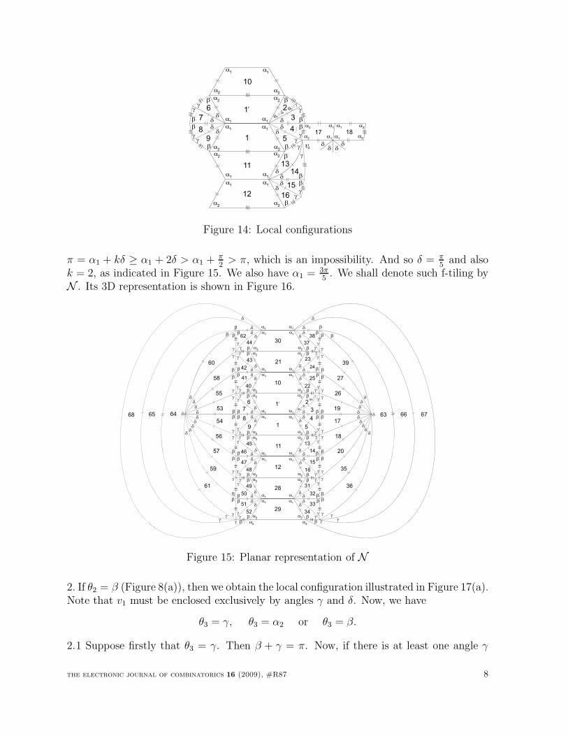
If x = α2, we obtain the configuration given in Figure 14. At vertex v4, one of thealternating angle sums must contain the sequence (. . . , β, γ, γ, . . .). But β + γ + γ > π,which is an impossibility.

If x = β, then α2 = β = π2

and consequently γ + δ > π2. It follows that a vertex

surrounded by six angles γ takes place, i.e., γ = π3. And so δ > π

6, since β + γ + δ > π.

The construction of the planar configuration is unique (Figure 15) and leads to a vertexsurrounded by only angles δ. Therefore δ = π

4or δ = π

5. However, if δ = π

4, then

the electronic journal of combinatorics 16 (2009), #R87 7

2

1

1’

a1

a1

a2

a2

a1

a1

a2

a2

g

3

4

5

6g

g

gg

7

8

9

g

g

dd

d

ddd

d

b

b

b

b

b

b

b

b

q1

dq2

g

a1

a1

a2

a2

10

a1

a1

a2

a2

11

12

a1

a1

a2

a2

13

g

14

15

16

g

g

dd

d

b

b

b

b

g

d

17a

1

a2

a2

a1

a1

a1

a2

a2

18

dd d

dv4

Figure 14: Local configurations

π = α1 + kδ ≥ α1 + 2δ > α1 + π2

> π, which is an impossibility. And so δ = π5

and alsok = 2, as indicated in Figure 15. We also have α1 = 3π

5. We shall denote such f-tiling by

N . Its 3D representation is shown in Figure 16.

31

29

28

a1

a1

a2

a2

a1

a1

a2

a2

g

32

33

34

g

g

dd

d

b

b

b

b

13

12

11

a1

a1

a2

a2

a1

a1

a2

a2

g

14

15

16

g

g

dd

d

b

b

b

b

g

d

d

49

g

50

51

52

g

g

dd

d

b

b

b

b

45

g

46

47

48

g

g

dd

d

b

b

b

b

g

d

d

g

2

1

1’

a1

a1

a2

a2

a1

a1

a2

a2

g

3

4

5

g

g

dd

d

b

b

b

b

q1

d

q2

g

23

10

21

a1

a1

a2

a2

a1

a1

a2

a2

g

24

25

22

g

g

dd

d

b

b

b

b

g

d

6

g

7

8

9

g

g

dd

d

b

b

b

b

43

g

42

41

40

g

g

dd

d

b

b

b

b

g

d

d

g

3730

a1

a1

a2

a2

38

g

d

b

b

g

d

44

62

g

d

b

b

g

d

g

d

g

g

g

b

b

b

b

g

g

b

b

g

g

b

b

g

g

b

dd

ddddd

d

36

35

20

18

17

19

26

27

39

d

g

g

g

b

b

b

b

g

g

b

b

g

g

b

b

g

g

b

dddd

dd

dd

61

59

57

56

54

53

55

58

60

dd

g g

b

b

b

b

6364

d

d

g g

6665

bg

d

a1

a1 d

a2

a2

b g

6768

Figure 15: Planar representation of N

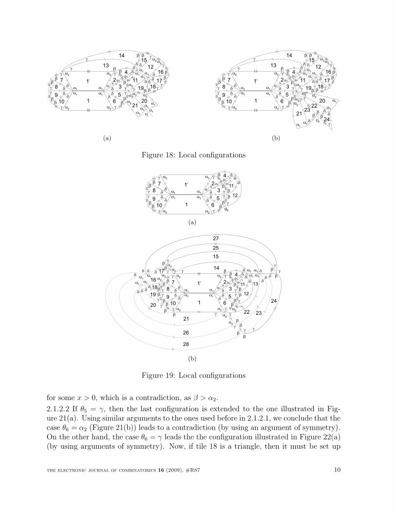
2. If θ2 = β (Figure 8(a)), then we obtain the local configuration illustrated in Figure 17(a).Note that v1 must be enclosed exclusively by angles γ and δ. Now, we have

θ3 = γ, θ3 = α2 or θ3 = β.

2.1 Suppose firstly that θ3 = γ. Then β + γ = π. Now, if there is at least one angle γ

the electronic journal of combinatorics 16 (2009), #R87 8

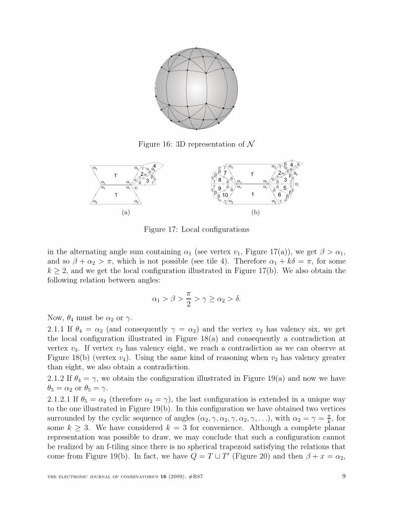
Figure 16: 3D representation of N

2

1

1’

a1

a1

a2

a2

a1

a1

a2

a2

3 gd

b

bq1

dq2

g q3

v1

4

(a)

2

1

1’

a1

a1

a2

a2

a1

a1

a2

a2

g

3

5

6

7

g

gg

g

8

9

10

gg

dd

d

ddd

d

b

b

bb

bb

bb

q1

dq2

g db 4

q4

v2

gq3

(b)

Figure 17: Local configurations

in the alternating angle sum containing α1 (see vertex v1, Figure 17(a)), we get β > α1,and so β + α2 > π, which is not possible (see tile 4). Therefore α1 + kδ = π, for somek ≥ 2, and we get the local configuration illustrated in Figure 17(b). We also obtain thefollowing relation between angles:

α1 > β >π

2> γ ≥ α2 > δ.

Now, θ4 must be α2 or γ.

2.1.1 If θ4 = α2 (and consequently γ = α2) and the vertex v2 has valency six, we getthe local configuration illustrated in Figure 18(a) and consequently a contradiction atvertex v3. If vertex v2 has valency eight, we reach a contradiction as we can observe atFigure 18(b) (vertex v4). Using the same kind of reasoning when v2 has valency greaterthan eight, we also obtain a contradiction.

2.1.2 If θ4 = γ, we obtain the configuration illustrated in Figure 19(a) and now we haveθ5 = α2 or θ5 = γ.

2.1.2.1 If θ5 = α2 (therefore α2 = γ), the last configuration is extended in a unique wayto the one illustrated in Figure 19(b). In this configuration we have obtained two verticessurrounded by the cyclic sequence of angles (α2, γ, α2, γ, α2, γ, . . .), with α2 = γ = π

k, for

some k ≥ 3. We have considered k = 3 for convenience. Although a complete planarrepresentation was possible to draw, we may conclude that such a configuration cannotbe realized by an f-tiling since there is no spherical trapezoid satisfying the relations thatcome from Figure 19(b). In fact, we have Q = T ∪ T ′ (Figure 20) and then β + x = α2,

the electronic journal of combinatorics 16 (2009), #R87 9

2

1

1’

a1

a1

a2

a2

a1

a1

a2

a2

g

3

5

6

7

g

gg

g

8

9

10

gg

dd

d

ddd

d

b

b

bb

bb

bb

q1

dq2

g d

b

4b dg

13

q4

a 2

14g

d

a2

a1 a

1

11

a1 a

1

a2a

2

12

b

d

g15

b

d ddd

g b b

b

b

gg

g

19 18

17

16

a2a

2a

2

a2 a

1a1a

1

a1

2021

v3

gq3

a1

(a)

2

1

1’

a1

a1

a2

a2

a1

a1

a2

a2

g

3

5

6

7

g

gg

g

8

9

10

gg

dd

d

ddd

d

b

b

bb

bb

bb

q1

dq2

g d

b

4b dg

13

q4

a 2

14g

d

a2

a1 a

1

11

a1 a

1

a2a

2

12

b

d

g15

b

d ddd

g b b

b

b

gg

g

19 18

17

16

a2

a2

a2

a2

a1

a1

a1a

1

20

21

v

2322

g g

bb d

db

d

g24

4

gq3

(b)

Figure 18: Local configurations

2

1

1’

a1

a1

a2

a2

a1

a1

a2

a2

g

3

5

6

7

g

gg

g

8

9

10

gg

dd

d

ddd

d

b

b

bb

bb

bb

q1

dq2

g d4

q4

bd

g

b11

g

b

d

12

q5

gq3

(a)

2

1

1’

a1

a1

a2

a2

a1

a1

a2

a2

g

3

5

6

7

g

gg

g

8

9

10

gg

dd

d

ddd

d

b

b

bb

bb

bb

q1

dq2

g d4

q4

bd

g

b11

g

b

d

12

q5a

2

a2

a1

a1

13

dg14

b

15

a2

a2 a

1a

1gb

da

2a

2

a1

a1

17

16g

bd 18

19

d

b

g

g

d

b

20

b21

g

d

d

g

b

22

d

bg

23a2

d

g

b

24

d b

g

25

26

a2

a1

a1

b

d

g

g

27

g

28

b

d

b

dg

q3

(b)

Figure 19: Local configurations

for some x > 0, which is a contradiction, as β > α2.

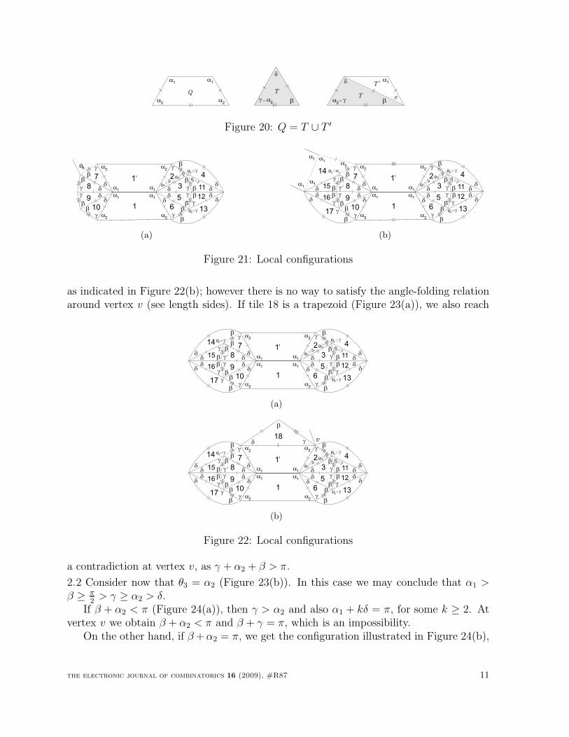
2.1.2.2 If θ5 = γ, then the last configuration is extended to the one illustrated in Fig-ure 21(a). Using similar arguments to the ones used before in 2.1.2.1, we conclude that thecase θ6 = α2 (Figure 21(b)) leads to a contradiction (by using an argument of symmetry).On the other hand, the case θ6 = γ leads the the configuration illustrated in Figure 22(a)(by using arguments of symmetry). Now, if tile 18 is a triangle, then it must be set up

the electronic journal of combinatorics 16 (2009), #R87 10

a1

a2 b

d

gT x

a1

a1

a2

a2 b

d

TQ

T ’

a2

g

Figure 20: Q = T ∪ T ′

2

1

1’

a1

a1

a2

a2

a1

a1

a2

a2

g

3

5

6

7

g

gg

g

8

9

10

gg

dd

d

ddd

d

b

b

bb

bb

bb

q1

dq2

g

d

4

b

dg

b 11

b

d

12

13

b

d

q6

q4 g

gq3

q5g

(a)

2

1

1’

a1

a1

a2

a2

a1

a1

a2

a2

g

3

5

6

7

g

gg

g

8

9

10

gg

dd

d

ddd

d

b

b

bb

bb

bb

q1

dq2

g

d

b

dg

b 11

b

d

12

b

dd

d g

b15

b16

17

b

g

d

g

a2

a1

a1

14

a1

a1

q6a

2

4

13

q4 g

gq3

q5g

(b)

Figure 21: Local configurations

as indicated in Figure 22(b); however there is no way to satisfy the angle-folding relationaround vertex v (see length sides). If tile 18 is a trapezoid (Figure 23(a)), we also reach

2

1

1’

a1

a1

a2

a2

a1

a1

a2

a2

g

3

5

6

7

g

gg

g

8

9

10

gg

dd

d

ddd

d

b

b

bb

bb

bb

q1

dq2

g

d

b

dg

b 11

b

d

12

b

dd

d g

b15

b16

17

b

g

d

g14

g

b

d

q6

4

13

q4 g

gq3

q5g

(a)

2

1

1’

a1

a1

a2

a2

a1

a1

a2

a2

g

3

5

6

7

g

gg

g

8

9

10

gg

dd

d

ddd

d

b

b

bb

bb

bb

q1

dq2

g

d

b

dg

b 11

b

d

12

b

dd

d g

b15

b16

17

b

g

d

g14

b

d

b

gd18 v

4

13

q4 g

gq3

q5g

gq6

(b)

Figure 22: Local configurations

a contradiction at vertex v, as γ + α2 + β > π.

2.2 Consider now that θ3 = α2 (Figure 23(b)). In this case we may conclude that α1 >

β ≥ π2

> γ ≥ α2 > δ.If β + α2 < π (Figure 24(a)), then γ > α2 and also α1 + kδ = π, for some k ≥ 2. At

vertex v we obtain β + α2 < π and β + γ = π, which is an impossibility.On the other hand, if β +α2 = π, we get the configuration illustrated in Figure 24(b),

the electronic journal of combinatorics 16 (2009), #R87 11

2

1

1’

a1

a1

a2

a2

a1

a1

a2

a2

g

3

5

6

7

g

gg

g

8

9

10

gg

dd

d

ddd

d

b

b

bb

bb

bb

q1

dq2

g

d

b

dg

b 11

b

d

12

b

dd

d g

b15

b16

17

b

g

d

g14

b

d

b

g

d

18

a2

a2

a1

a1

19

v

4

13

q4 g

gq3

q5g

gq6

a1

a1

(a)

2

1

1’

a1

a1

a2

a2

a1

a1

a2

a2

3 gd

b

bq1

dq2

g a2q3

a2

a1

a1

4

(b)

Figure 23: Local configurations

2

1

1’

a1

a1

a2

a2

a1

a1

a2

a2

3 gd

b

bq1

dq2

g a2q3

a2

a1

a1

4

5g d

bv

a1

a1

(a)

2

1

1’

a1

a1

a2

a2

a1

a1

a2

a2

3 gd

b

bq1

dq2

g a2q3

a2

a1

a1

4

5g

d

b

g

86

7g

g

d

dd

b

bb 9

b

d

g

a1

a1

(b)

Figure 24: Local configurations

with α2 = γ, and α1 + kδ = π, for some k ≥ 2. As in 2.1.2.1, we obtain a contradiction.

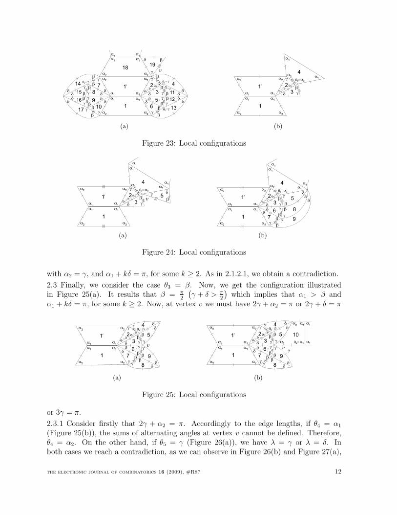
2.3 Finally, we consider the case θ3 = β. Now, we get the configuration illustratedin Figure 25(a). It results that β = π

2

(

γ + δ > π2

)

which implies that α1 > β andα1 + kδ = π, for some k ≥ 2. Now, at vertex v we must have 2γ + α2 = π or 2γ + δ = π

2

1

1’

a1

a1

a2

a2

a1

a1

a2

a2

3 gd

b

bq1

dq2

g q3

4

5

g

d

b

g

6

7

g

g

d

dd b

b

b

9

8g db

g

d

b

v

(a)

2

1

1’

a1

a1

a2

a2

a1

a1

a2

a2

3 gd

b

bq1

dq2

g q3

4

5

g

d

b

g

6

7

g

g

d

dd b

b

b

9

8g db

g

d

b

a2

a2

a1

10

vq4

a1

a1

a1

?

(b)

Figure 25: Local configurations

or 3γ = π.

2.3.1 Consider firstly that 2γ + α2 = π. Accordingly to the edge lengths, if θ4 = α1

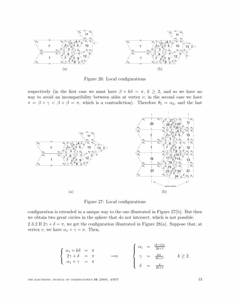
(Figure 25(b)), the sums of alternating angles at vertex v cannot be defined. Therefore,θ4 = α2. On the other hand, if θ5 = γ (Figure 26(a)), we have λ = γ or λ = δ. Inboth cases we reach a contradiction, as we can observe in Figure 26(b) and Figure 27(a),

the electronic journal of combinatorics 16 (2009), #R87 12

2

1

1’

a1

a1

a2

a2

a1

a1

a2

a2

3 gd

b

bq1

dq2

gq3

4

5

g

b

g

6

7

g

g

d

dd b

b

b

9

8g db

g

b

a2

a1

a1

10

12

d

d

a1

a1

a2

a2

11

q4a

2

q5

l

g

d

b

(a)

2

1

1’

a1

a1

a2

a2

a1

a1

a2

a2

3 gd

b

bq1

dq2

gq3

4

5

g

b

g

6

7

g

g

d

dd b

b

b

9

8g db

g

b

a2

a1

a1

10

12

d

d

a1

a1

a2

a2

11

q4a

2

q5

l

g

d

b

g

d

b13

d

v

(b)

Figure 26: Local configurations

respectively (in the first case we must have β + kδ = π, k ≥ 2, and so we have noway to avoid an incompatibility between sides at vertex v; in the second case we haveπ = β + γ < β + β = π, which is a contradiction). Therefore θ5 = α2, and the last

2

1

1’

a1

a1

a2

a2

a1

a1

a2

a2

3 gd

b

bq1

dq2

gq3

4

5

g

b

g

6

7

g

g

d

dd b

b

b

9

8g db

g

b

a2

a1

a1

10

12

d

d

a1

a1

a2

a2

11

q4a

2

q5

l

g

d

b

g

d

b13

v

(a)

2

1

1’

a1

a1

a2

a2

a1

a1

a2

a2

3 gd

b

bq1

dq2

gq3

4

5

g

d

b

g

6

7

g

g

d

dd b

b

b

9

8g db

g

d

b

a2

a1

a1

10

a2

a1

a1

12

17

22

16

a1

a1

a2

a2

a1

a1

a2

a2

18 gd

b

g

15

g

d

b

g

19

23

g

g

d

dd b

b 20

24g db

g

d

b

a2

a1

a2

a1

13

a2

a2

a1

a1

21

b14

d

a1

a1

2829

a1a

1

a2

a2

27gd

b

g

25

g

b

gd

a2

a2

11

b26

d

b

d

b

q4a

2

great circles

q5a

2

(b)

Figure 27: Local configurations

configuration is extended in a unique way to the one illustrated in Figure 27(b). But thenwe obtain two great circles in the sphere that do not intersect, which is not possible.

2.3.2 If 2γ + δ = π, we get the configuration illustrated in Figure 28(a). Suppose that, atvertex v, we have α1 + γ = π. Then,

α1 + kδ = π

2γ + δ = π

α1 + γ = π

=⇒

α1 = (k+1)π2k+1

γ = kπ2k+1

,

δ = π2k+1

k ≥ 2.

the electronic journal of combinatorics 16 (2009), #R87 13

The relation between angles is given by

α1 > β = π2

> γ > δ

α1 > α2 > γ > δ.

Considering a vertex surrounded by the cyclic sequence (α2, γ, γ, . . .), we obtain α2+γ < π

and α2+γ+ρ ≥ α2+γ+δ > 2kπ2k+1

+ π2k+1

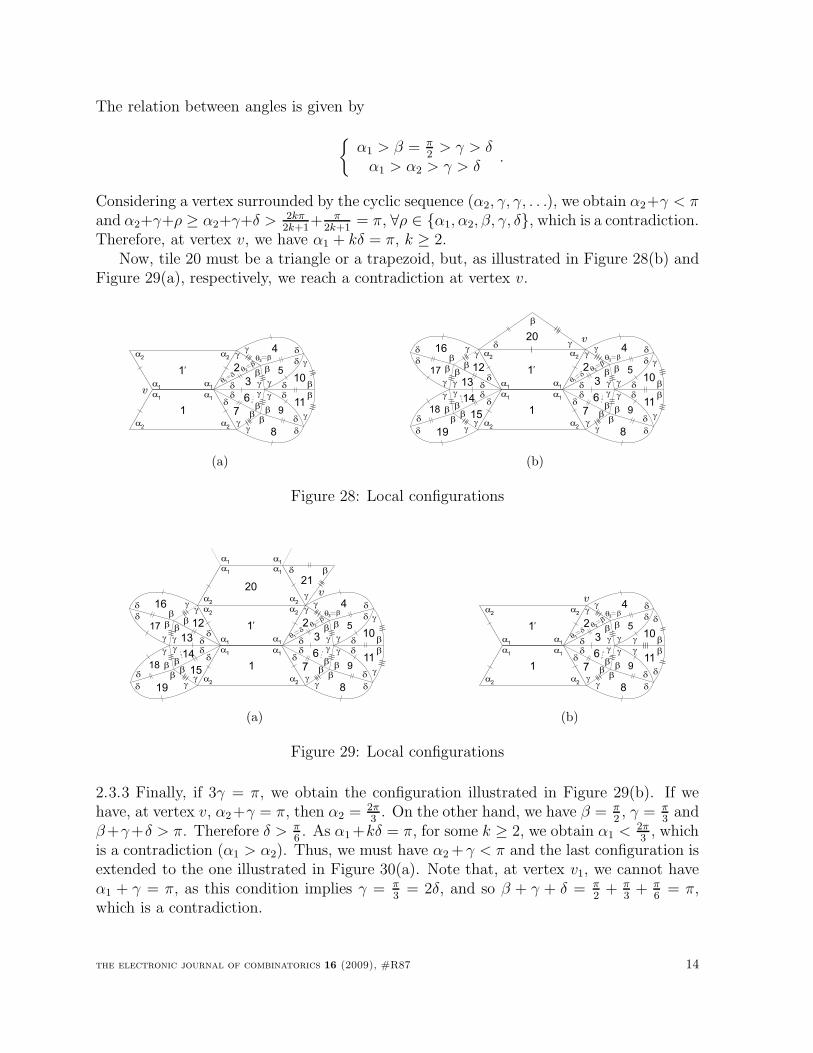
= π, ∀ρ ∈ α1, α2, β, γ, δ, which is a contradiction.Therefore, at vertex v, we have α1 + kδ = π, k ≥ 2.

Now, tile 20 must be a triangle or a trapezoid, but, as illustrated in Figure 28(b) andFigure 29(a), respectively, we reach a contradiction at vertex v.

2

1

1’

a1

a1

a2

a2

a1

a1

a2

a2

g

3

6

7

gg

dd

d

b

b

bb

q1

dq2

gg

d

4

d

g

b 5

b

d

9

8

bg

d g

dd

b

b

g

g

10

11

v

q3b

(a)

2

1

1’

a1

a1

a2

a2

a1

a1

a2

a2

g

3

6

7

gg

dd

d

b

b

bb

q1

dq2

gg

d

4

d

g

b 5

b

d

9

8

bg

d g

20

dd

b

b

g

g

10

11

12

g

13

14

15

gg

dd

d

b

bb

gg

d

16b

d

g

b17

b

d

18

19

bg

d

gd

b

b

gdv

q3b

(b)

Figure 28: Local configurations

2

1

1’

a1

a1

a2

a2

a1

a1

a2

a2

g

3

6

7

gg

dd

d

b

b

bb

q1

dq2

gg

d

4

d

g

b 5

b

d

9

8

bg

d g

b

g

d

20

a2

a2

a1

a1

21

v

dd

b

b

g

g

10

11

12

g

13

14

15

gg

dd

d

b

bb

gg

d

16b

d

g

b17

b

d

18

19

bg

d

gd

bq3

b

a1

a1

(a)

2

1

1’

a1

a1

a2

a2

a1

a1

a2

a2

g

3

6

7

gg

dd

d

b

b

bb

q1

dq2

gg

d

4

d

g

b 5

b

d

9

8

bg

d

g

d

d

b

b

g

g

10

11

v

q3b

(b)

Figure 29: Local configurations

2.3.3 Finally, if 3γ = π, we obtain the configuration illustrated in Figure 29(b). If wehave, at vertex v, α2+γ = π, then α2 = 2π

3. On the other hand, we have β = π

2, γ = π

3and

β+γ+δ > π. Therefore δ > π6. As α1 +kδ = π, for some k ≥ 2, we obtain α1 < 2π

3, which

is a contradiction (α1 > α2). Thus, we must have α2 +γ < π and the last configuration isextended to the one illustrated in Figure 30(a). Note that, at vertex v1, we cannot haveα1 + γ = π, as this condition implies γ = π

3= 2δ, and so β + γ + δ = π

2+ π

3+ π

6= π,

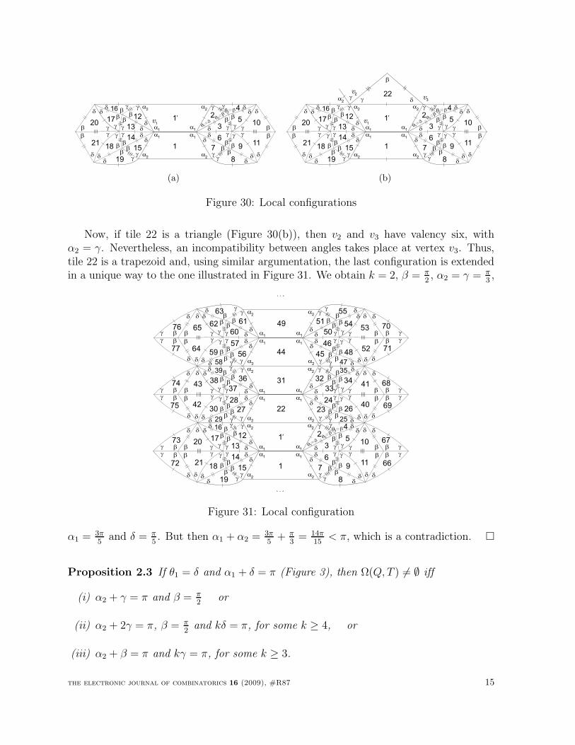
which is a contradiction.

the electronic journal of combinatorics 16 (2009), #R87 14

1

1’

d

2

a1

a1

a2

a2

a1

a1

a2

a2

3 gd

b

g

5g

b

g

6

7

g

g

d

dd b

b 9

8g db

g

d

b

10

4b

q1

dq2

q3b

gg

d

d

b

b

11

d

12

13g d

b

g

17g

b

g

14

15

g

g

d

ddb

b18

19 gdb

g

d

b

20

16

gg

d

d

b

b

21

bb

d v1

(a)

1

1’

d

2

a1

a1

a2

a2

a1

a1

a2

a2

3 gd

b

g

5g

b

g

6

7

g

g

d

dd b

b 9

8g db

g

d

b

10

4b

q1

dq2

q3b

gg

d

d

b

b

11

d

12

13g d

b

g

17g

b

g

14

15

g

g

d

ddb

b18

19 gdb

g

d

b

20

16

gg

d

d

b

b

21

bb

d v1

22

b

g d v3a

2gv

2

(b)

Figure 30: Local configurations

Now, if tile 22 is a triangle (Figure 30(b)), then v2 and v3 have valency six, withα2 = γ. Nevertheless, an incompatibility between angles takes place at vertex v3. Thus,tile 22 is a trapezoid and, using similar argumentation, the last configuration is extendedin a unique way to the one illustrated in Figure 31. We obtain k = 2, β = π

2, α2 = γ = π

3,

32

1

1’

a1

a1

a2

a2

a1

a1

a2

a2

33gd

b

g 35

34

g

b

g

24

23

g

g

d

dd b

b 26

25g db

g

d

b

41

40

2

22

31

a1

a1

a2

a2

a1

a1

a2

a2

3 gd

b

g

5g

d

b

g

6

7

g

g

d

dd b

b 9

8g db

g

d

b

10

66

4

d

51

a1

a1

a2

a2

a1

a1

a2

a2

50 gd

b

g 55

54g

b

g

46

45

g

g

d

dd b

b 48

47g db

g

b

53

5244

49

d

d

b

q1

dq2

q3b

gg

d

d

b

b

b

b

d

d

g

g

11

67

bb

dgg

d

d

b

b

69

b

b

d

d

g

g

68

d

bb

gg

d

d

b

b

71

b

b

d

d

g

g

70

36

37g d

b

g39

38

g

b

g

28

27

g

g

d

ddb

b30

29 gd b

g

d

b

43

42

12

13g d

b

g

17g

d

b

g

14

15

g

g

d

ddb

b18

19 gdb

g

d

b

20

72

16

d

61

60g d

b

g63

62g

b

g

57

56

g

g

d

ddb

b59

58 gd b

g

b

65

64

d

d

gg

d

d

b

b

b

b

d

d

g

g

21

73

bb

dgg

d

d

b

b

75

b

b

d

d

g

g

74

d

bb

gg

d

d

b

b

77

b

b

d

d

g

g

76

bb

d

Figure 31: Local configuration

α1 = 3π5

and δ = π5. But then α1 + α2 = 3π

5+ π

3= 14π

15< π, which is a contradiction.

Proposition 2.3 If θ1 = δ and α1 + δ = π (Figure 3), then Ω(Q, T ) 6= ∅ iff

(i) α2 + γ = π and β = π2

or

(ii) α2 + 2γ = π, β = π2

and kδ = π, for some k ≥ 4, or

(iii) α2 + β = π and kγ = π, for some k ≥ 3.

the electronic journal of combinatorics 16 (2009), #R87 15

The first case leads to a family of f-tilings, denoted by R2δγ , with δ, γ ∈

(

0, π2

)

. A planarrepresentation is given in Figure 38(a). For its 3D representation see Figure 38(b).The case (ii) leads to a family of f-tilings, denoted by Mk

γ, with

γ ∈

(

(k − 2)π

2k,1

2arccos

(

− cos2 π

k

)

)

.

In Figure 41 is given the corresponding planar representation. 3D representations fork = 4 and k = 5 are given in Figure 42.In the last situation, there is a family of f-tilings, denoted by Rk

δβ, with

β + δ ∈(

(k−1)πk

, πk

+ arccos(

− cos2 πk

)

)

and k ≥ 3. A planar representation is given in

Figure 52. For their k = 3, k = 4 and k = 5 3D representations see Figure 53.

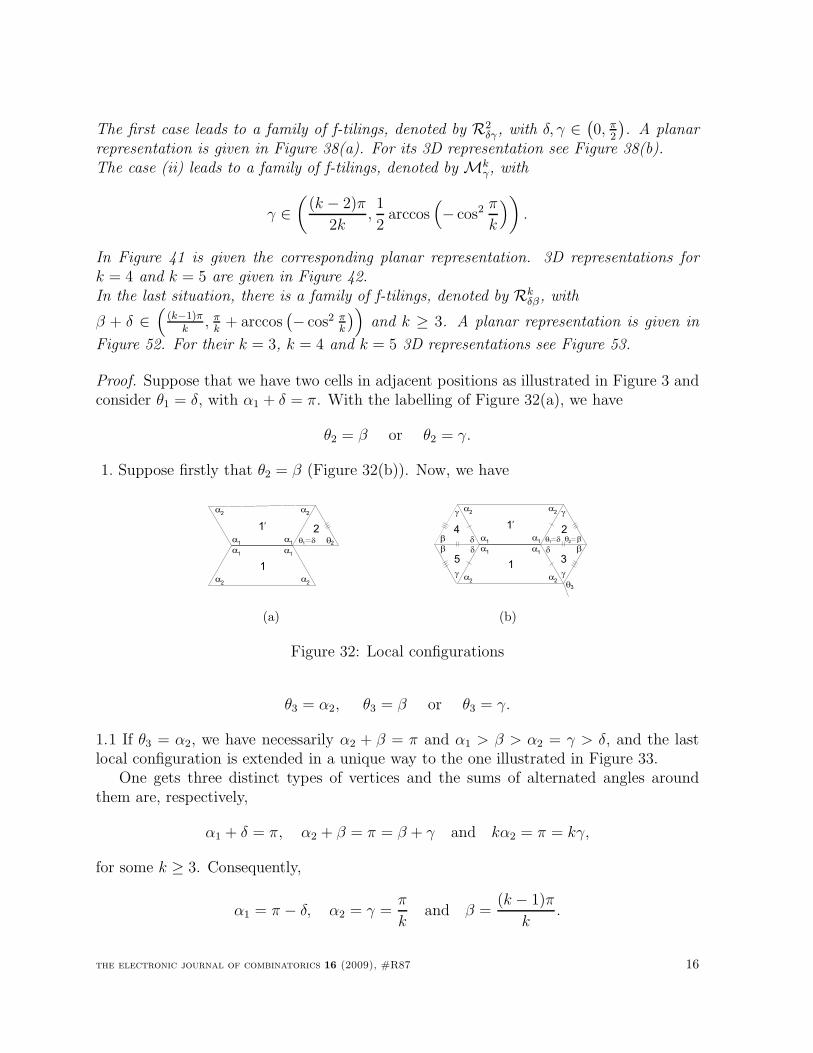
Proof. Suppose that we have two cells in adjacent positions as illustrated in Figure 3 andconsider θ1 = δ, with α1 + δ = π. With the labelling of Figure 32(a), we have

θ2 = β or θ2 = γ.

1. Suppose firstly that θ2 = β (Figure 32(b)). Now, we have

2

1

1’

a1

a1

a2

a2

a1

a1

a2

a2

q2q1d

(a)

2

3

b

1

1’

q

a1

a1

a2

a2

a1

a1

a2

a2

3

g

q2

d

q1bd

g

4

5

b

g

d

g

b d

(b)

Figure 32: Local configurations

θ3 = α2, θ3 = β or θ3 = γ.

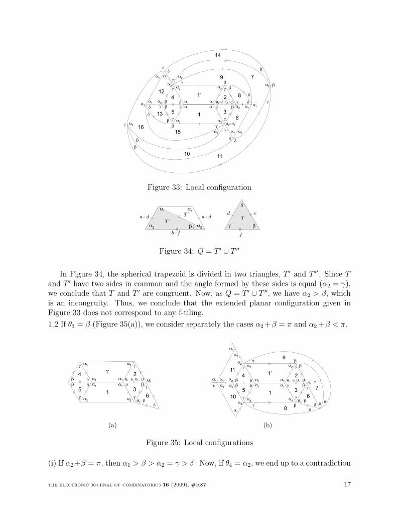
1.1 If θ3 = α2, we have necessarily α2 + β = π and α1 > β > α2 = γ > δ, and the lastlocal configuration is extended in a unique way to the one illustrated in Figure 33.

One gets three distinct types of vertices and the sums of alternated angles aroundthem are, respectively,

α1 + δ = π, α2 + β = π = β + γ and kα2 = π = kγ,

for some k ≥ 3. Consequently,

α1 = π − δ, α2 = γ =π

kand β =

(k − 1)π

k.

the electronic journal of combinatorics 16 (2009), #R87 16

2

3

b

1

1’

a1

a1

a2

a2

a1

a1

a2

a2

g

q2

d

q1bd

g

4

5

b

g

d

g

b d

q3a

2

a1

a1

6

a2

8

a1

a1

12

a2

g b

d

9

b

d

13

gb

d

15

g

b

d

a2

a1

a1

a1

a1

a2

a2

a2

a2

7g

db

g

b d

10

d

b

g

11

14

16

d

g

b

g

Figure 33: Local configuration

a1

a1

a2

a2 b

d

g

Td

f

e

T ’dada

fb

T ’’

b

Figure 34: Q = T ′ ∪ T ′′

In Figure 34, the spherical trapezoid is divided in two triangles, T ′ and T ′′. Since T

and T ′ have two sides in common and the angle formed by these sides is equal (α2 = γ),we conclude that T and T ′ are congruent. Now, as Q = T ′ ∪ T ′′, we have α2 > β, whichis an incongruity. Thus, we conclude that the extended planar configuration given inFigure 33 does not correspond to any f-tiling.

1.2 If θ3 = β (Figure 35(a)), we consider separately the cases α2 +β = π and α2 +β < π.

2

3

b

1

1’

a1

a1

a2

a2

a1

a1

a2

a2

g

q2

d

q1bd

g

4

5

b

g

d

g

b d

g

q3

6

db

q4

(a)

2

3

b

1

1’

a1

a1

a2

a2

a1

a1

a2

a2

g

q2

d

q1bd

g

4

5

b

g

d

g

b d

g

q3

6

db

q4g

b

d

7

8b

d

g

bg

d

9

a1

a1

10

a2

a2

a1

a1

11

a2

a2

v

a1

a1

(b)

Figure 35: Local configurations

(i) If α2+β = π, then α1 > β > α2 = γ > δ. Now, if θ4 = α2, we end up to a contradiction

the electronic journal of combinatorics 16 (2009), #R87 17

since we obtain the planar representation given in Figure 33 (in a symmetrical way). Onthe other hand, if θ4 = γ, we reach an impossibility at vertex v, see Figure 35(b).

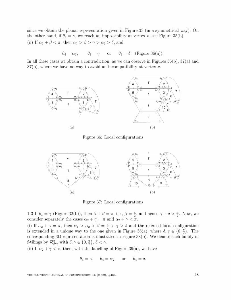
(ii) If α2 + β < π, then α1 > β > γ > α2 > δ, and

θ4 = α2, θ4 = γ or θ4 = δ (Figure 36(a)).

In all these cases we obtain a contradiction, as we can observe in Figures 36(b), 37(a) and37(b), where we have no way to avoid an incompatibility at vertex v.

2

3

b

1

1’

a1

a1

a2

a2

a1

a1

a2

a2

g

q2

d

q1bd

g

4

5

b

g

d

g

b d

g

q3

6

db

b

d

7

q4

g

(a)

2

3

b

1

1’

a1

a1

a2

a2

a1

a1

a2

a2

g

q2q1bd

g

4

5

b

g

d

g

b d

g

q3

6

db

b

d

7

g

8

a1

a1

a2 q4

a2

9

v

a2

a1

a1

a2

d

d

g

b10

(b)

Figure 36: Local configurations

2

3

b

1

1’

a1

a1

a2

a2

a1

a1

a2

a2

g

q2

d

q1bd

g

4

5

b

g

d

g

b d

g

q3

6

db

b

d

7

g

8

q4

b

gd v

(a)

2

3

ba1

a1

a2

a2

a1

a1

a2

a2

g

q2

d

q1bd

g

4

5

b

g

d

g

b d

g

q3

6

db

b

d

7

g

8

q4

b

g d

1

1’

910

d

d gg

b

b

v

(b)

Figure 37: Local configurations

1.3 If θ3 = γ (Figure 32(b)), then β + β = π, i.e., β = π2, and hence γ + δ > π

2. Now, we

consider separately the cases α2 + γ = π and α2 + γ < π.

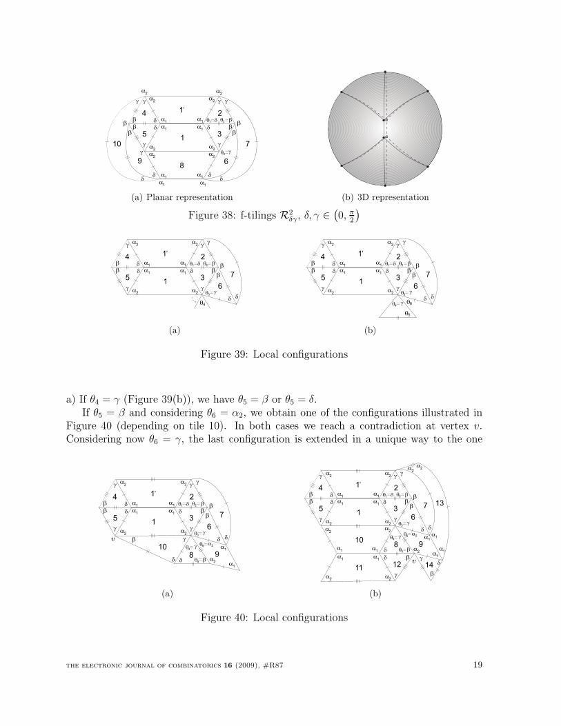
(i) If α2 + γ = π, then α1 > α2 > β = π2

> γ > δ and the refereed local configurationis extended in a unique way to the one given in Figure 38(a), where δ, γ ∈

(

0, π2

)

. Thecorresponding 3D representation is illustrated in Figure 38(b). We denote such family off-tilings by R2

δγ , with δ, γ ∈(

0, π2

)

, δ < γ.

(ii) If α2 + γ < π, then, with the labelling of Figure 39(a), we have

θ4 = γ, θ4 = α2 or θ4 = δ.

the electronic journal of combinatorics 16 (2009), #R87 18

2

3

b

1

1’

a1

a1

a2

a2

a1

a1

a2

a2

g

q2

d

q1bd

g

4

5

b

g

d

g

b d

gq3

6

d

b

b

d

7

g

8

a1

a1

a2

a2

9

d

b

b

d

10

g

a1

a1

a2

a2

g

(a) Planar representation (b) 3D representation

Figure 38: f-tilings R2δγ , δ, γ ∈

(

0, π2

)

2

3

b

1

1’

a1

a1

a2

a2

a1

a1

a2

a2

g

q2

d

q1bd

g

4

5

b

g

d

g

b d

gq3

6

d

b

b

d

7

g

q4

(a)

2

3

b

1

1’

a1

a1

a2

a2

a1

a1

a2

a2

g

q2

d

q1bd

g

4

5

b

g

d

g

b d

gq3

6

d

b

b

d

7

g

gq4

q5

q6

(b)

Figure 39: Local configurations

a) If θ4 = γ (Figure 39(b)), we have θ5 = β or θ5 = δ.If θ5 = β and considering θ6 = α2, we obtain one of the configurations illustrated in

Figure 40 (depending on tile 10). In both cases we reach a contradiction at vertex v.Considering now θ6 = γ, the last configuration is extended in a unique way to the one

2

3

b

1

1’

a1

a1

a2

a2

a1

a1

a2

a2

g

q2

d

q1bd

g

4

5

b

g

d

g

b d

gq3

6

d

b

b

d

7

g

gq4

q5bd

8

q6a

2

a2

a1

a1

9

b

d

g

10

v

(a)

2

3

b

1

1’

a1

a1

a2

a2

a1

a1

a2

a2

g

q2

d

q1bd

g

4

5

b

g

d

g

b d

gq3

6

d

b

b

d

7

g

gq4

q5bd

8

a2

a1

a1

10

a2

11

a1

a1

a2

a2

d b

g

12

q6a

2

a2

a1

a1

9

v

a1

a1

a2a

2

13

dg

b

14

(b)

Figure 40: Local configurations

the electronic journal of combinatorics 16 (2009), #R87 19

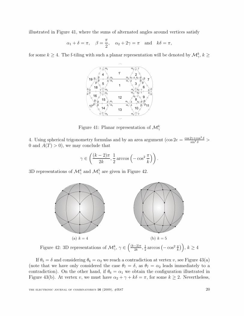
illustrated in Figure 41, where the sums of alternated angles around vertices satisfy

α1 + δ = π, β =π

2, α2 + 2γ = π and kδ = π,

for some k ≥ 4. The f-tiling with such a planar representation will be denoted by Mkγ, k ≥

2

3

b

1

1’

a1

a1

a2

a2

a1

a1

a2

a2

g

q2

d

q1bd

g

4

5

b

g

d

g

b d

gq3

6d

b

b

d

7

g

gq4

q5bd

8

a2

a1

a1

12

a2 d

b

gq6

9

13

a1

a1

a2

a2

d b

g

10

b

d

g

11

18

d

b

b

d

19

g

d15

d

b

16

db

g

14

b

d

g

17

g

gg

b

Figure 41: Planar representation of Mkγ

4. Using spherical trigonometry formulas and by an area argument (cos 2e = cos 2γ+cos2 δ

sin2 δ>

0 and A(T ) > 0), we may conclude that

γ ∈

(

(k − 2)π

2k,1

2arccos

(

− cos2 π

k

)

)

.

3D representations of M4γ and M5

γ are given in Figure 42.

(a) k = 4 (b) k = 5

Figure 42: 3D representations of Mkγ, γ ∈

(

(k−2)π2k

, 12arccos

(

− cos2 πk

)

)

, k ≥ 4

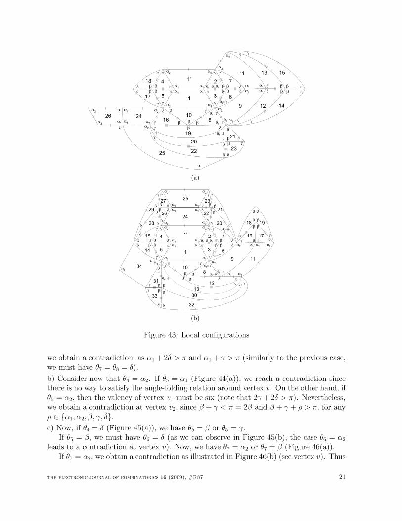
If θ5 = δ and considering θ6 = α2 we reach a contradiction at vertex v, see Figure 43(a)(note that we have only considered the case θ7 = δ, as θ7 = α2 leads immediately to acontradiction). On the other hand, if θ6 = α1 we obtain the configuration illustrated inFigure 43(b). At vertex v, we must have α2 + γ + kδ = π, for some k ≥ 2. Nevertheless,

the electronic journal of combinatorics 16 (2009), #R87 20

2

3

b

1

1’

a1

a1

a2

a2

a1

a1

a2

a2

g

q2

d

q1bd

g

4

5

b

g

d

g

b d

gq4

q5 d

gq3

6

db

b d

g

7

17

d b

bd

g

18

g

b

d g

10

b8

a2

a1

a1

q6a

2

a1

a1

a2

a2

9

11

d

d

b

b

g

g

13

12

b

b

d

d

g

g

15

14

g b16

d

b dg

19d

dq7

g

b20

b g21

b b g

dd

g

2223

a2

a1

25

v

a2

a2

a1

a1

a2

a2

a1

a1

2426

(a)

2

3

b

1

1’

a1

a1

a2

a2

a1

a1

a2

a2

g

q2

d

q1bd

g

4

5

b

g

d

g

b d

gq4

q5 d

gq3

6

db

b d

g

7

14

d b

bd

g

15

g

b

d g

10

b8

a2

a2

a1

q6a

1

9

21

d

b

g16

11

b

d g17

g

b

13

d

b d g

12

g

bd

24

25

a1

a1

a2

a1

a1

a2

a2

22

v

a1

a1

a2

a2

d

b

g

18b

d

g

19

q7 d

d20g

b

bbd

gg

23

29

g

b d26

d 28 g

b

b b d

g g

27

d

33

d

b

d

30

g g

q8 d

d

31b

bbgg

32

a2

34a

1

a2

(b)

Figure 43: Local configurations

we obtain a contradiction, as α1 + 2δ > π and α1 + γ > π (similarly to the previous case,we must have θ7 = θ8 = δ).

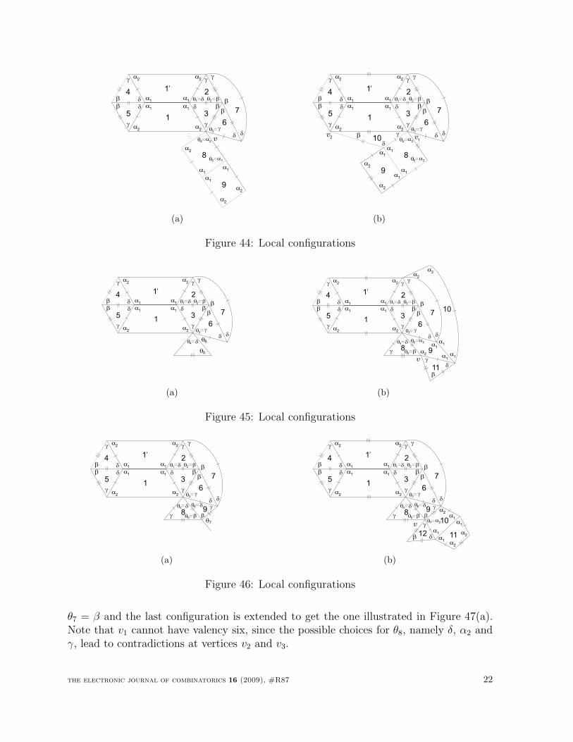
b) Consider now that θ4 = α2. If θ5 = α1 (Figure 44(a)), we reach a contradiction sincethere is no way to satisfy the angle-folding relation around vertex v. On the other hand, ifθ5 = α2, then the valency of vertex v1 must be six (note that 2γ + 2δ > π). Nevertheless,we obtain a contradiction at vertex v2, since β + γ < π = 2β and β + γ + ρ > π, for anyρ ∈ α1, α2, β, γ, δ.

c) Now, if θ4 = δ (Figure 45(a)), we have θ5 = β or θ5 = γ.If θ5 = β, we must have θ6 = δ (as we can observe in Figure 45(b), the case θ6 = α2

leads to a contradiction at vertex v). Now, we have θ7 = α2 or θ7 = β (Figure 46(a)).If θ7 = α2, we obtain a contradiction as illustrated in Figure 46(b) (see vertex v). Thus

the electronic journal of combinatorics 16 (2009), #R87 21

2

3

b

1

1’

a1

a1

a2

a2

a1

a1

a2

a2

g

q2

d

q1bd

g

4

5

b

g

d

g

b d

gq3

6

d

b

b

d

7

g

9

a1

a2

8

a2

q4

a1q5

a1

a2

a2

a1

v

(a)

2

3

b

1

1’

a1

a1

a2

a2

a1

a1

a2

a2

g

q2

d

q1bd

g

4

5

b

g

d

g

b d

gq3

6

d

b

b

d

7

g

a1

9

a2

a1

a2

8

a1

q4

a2q5

a1

a2

10d

gbv v1

2

(b)

Figure 44: Local configurations

2

3

b

1

1’

a1

a1

a2

a2

a1

a1

a2

a2

g

q2

d

q1bd

g

4

5

b

g

d

g

b d

gq3

6

d

b

b

d

7

g

dq4

q5

q6

(a)

2

3

b

1

1’

a1

a1

a2

a2

a1

a1

a2

a2

g

q2

d

q1bd

g

4

5

b

g

d

g

b d

gq3

6

d

b

b

d

7

g

bq5

dq4

g 8

q6a

2

a2

a1

a1

9

a1

a1

a2a

2

10

vd

g

b11

(b)

Figure 45: Local configurations

2

3

b

1

1’

a1

a1

a2

a2

a1

a1

a2

a2

g

q2

d

q1bd

g

4

5

b

g

d

g

b d

gq3

6

d

b

b

d

7

g

bq5

dq4

g 8

q6

9d

b

g

q7

(a)

2

3

b

1

1’

a1

a1

a2

a2

a1

a1

a2

a2

g

q2

d

q1bd

g

4

5

b

g

d

g

b d

gq3

6

d

b

b

d

7

g

bq5

dq4

g 8

q6

a2

9

10v

d

g

b 12

d

b

g

a2q7

a1

a1

a2

11

a1

a1

a2

(b)

Figure 46: Local configurations

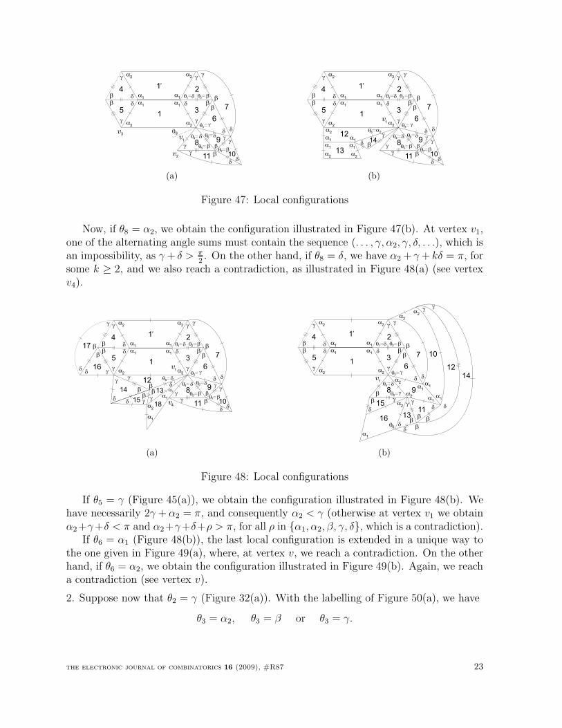
θ7 = β and the last configuration is extended to get the one illustrated in Figure 47(a).Note that v1 cannot have valency six, since the possible choices for θ8, namely δ, α2 andγ, lead to contradictions at vertices v2 and v3.

the electronic journal of combinatorics 16 (2009), #R87 22

2

3

b

1

1’

a1

a1

a2

a2

a1

a1

a2

a2

g

q2

d

q1bd

g

4

5

b

g

d

g

b d

gq3

6

d

b

b

d

7

g

bq5

dq4

g 8

q6

9

10

d

g b

d

b

g

bq7

11

g

d

q8

v2

v1

v3

(a)

2

3

b

1

1’

a1

a1

a2

a2

a1

a1

a2

a2

g

q2

d

q1bd

g

4

5

b

g

d

g

b d

gq3

6

d

b

b

d

7

g

bq5

dq4

g 8

q6

9

10

d

g b

d

b

g

bq7

11

g

d

v1

a2q8

a2

a1

a1

a1

a1

a2

a2

g

d b

12

13

14

(b)

Figure 47: Local configurations

Now, if θ8 = α2, we obtain the configuration illustrated in Figure 47(b). At vertex v1,one of the alternating angle sums must contain the sequence (. . . , γ, α2, γ, δ, . . .), which isan impossibility, as γ + δ > π

2. On the other hand, if θ8 = δ, we have α2 + γ + kδ = π, for

some k ≥ 2, and we also reach a contradiction, as illustrated in Figure 48(a) (see vertexv4).

2

3

b

1

1’

a1

a1

a2

a2

a1

a1

a2

a2

g

q2

d

q1bd

g

4

5

b

g

d

g

b d

gq3

6

d

b

b

d

7

g

bq5

dq4

g 8

q6

9

10

d

g b

d

b

g

bq7

11

g

d

v1

q8g

db12

1314

d

gbb

b

g

dd g15

g

b

d16

17 b

d

g

a2

a2

a1

a1

18 v4

(a)

2

3

b

1

1’

a1

a1

a2

a2

a1

a1

a2

a2

g

q2

d

q1bd

g

4

5

b

g

d

g

b d

gq3

6

d

b

b

d

7

g

gq5

dq4

b8

a2

a1

a1

9

a1

a1

a2a

2

10

dg

b11

a2

d

b

g

12

g

bd

13

bd

g

14

gb

d15 a

2

16q6

a1

v1

(b)

Figure 48: Local configurations

If θ5 = γ (Figure 45(a)), we obtain the configuration illustrated in Figure 48(b). Wehave necessarily 2γ + α2 = π, and consequently α2 < γ (otherwise at vertex v1 we obtainα2+γ+δ < π and α2+γ+δ+ρ > π, for all ρ in α1, α2, β, γ, δ, which is a contradiction).

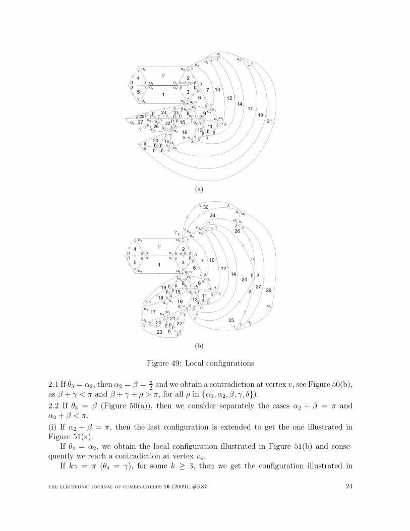
If θ6 = α1 (Figure 48(b)), the last local configuration is extended in a unique way tothe one given in Figure 49(a), where, at vertex v, we reach a contradiction. On the otherhand, if θ6 = α2, we obtain the configuration illustrated in Figure 49(b). Again, we reacha contradiction (see vertex v).

2. Suppose now that θ2 = γ (Figure 32(a)). With the labelling of Figure 50(a), we have

θ3 = α2, θ3 = β or θ3 = γ.

the electronic journal of combinatorics 16 (2009), #R87 23

2

3

b

1

1’

a1

a1

a2

a2

a1

a1

a2

a2

g

q2

d

q1bd

g

4

5

b

g

d

g

b d

gq3

6

d

b

b

d

7

g

gq5

dq4

b8

a2

a1

a1

9

a1

a1

a2a

2

10

dg

b11

a2

d

b

g

12

g

bd

13

bd

g

14

gb

d15 a

2

d

bg

16

bg

d

q6a

1

a2

a1

a1

a2

a2

a1

17

db

g

18

db

g

19

20

g

bd

b

21

d

g

22

23

d

gb

25 gbd

24

27

26

a2

a2

a2a

1

a1

a1

v?

(a)

2

3

b

1

1’

a1

a1

a2

a2

a1

a1

a2

a2

g

q2

d

q1bd

g

4

5

b

g

d

g

b d

gq3

6

d

b

b

d

7

g

gq5

dq4

b8

a2

a1

a1

9

a1

a1

a2a

2

10

dg

b11

a2

d

b

g

12

g

bd

13

bd

g

14

gb

d15 a

2

16

a1

v

q6a

2

a1a

1

a1

a2

a2

17

18 d

b

g

b

d

g

19

2120

d d

g

g

b b 22

dd

g

bb

23

g

g

b

24

d

b

g

25

g

b

26

d

b

27

d

g

a2

a2

a1

a1 a

1

a128

a2

a2

29

db30

g

?

d

(b)

Figure 49: Local configurations

2.1 If θ3 = α2, then α2 = β = π2

and we obtain a contradiction at vertex v, see Figure 50(b),as β + γ < π and β + γ + ρ > π, for all ρ in α1, α2, β, γ, δ).

2.2 If θ3 = β (Figure 50(a)), then we consider separately the cases α2 + β = π andα2 + β < π.

(i) If α2 + β = π, then the last configuration is extended to get the one illustrated inFigure 51(a).

If θ4 = α2, we obtain the local configuration illustrated in Figure 51(b) and conse-quently we reach a contradiction at vertex v4.

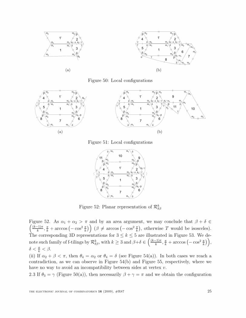
If kγ = π (θ4 = γ), for some k ≥ 3, then we get the configuration illustrated in

the electronic journal of combinatorics 16 (2009), #R87 24

2

3

b1

1’

q

a1

a1

a2

a2

a1

a1

a2

a2

3

g

gd q2

d

q1

b

(a)

2

3

b1

1’

a1

a1

a2

a2

a1

a1

a2

a2

g

gd q2

d

q1

b

q3a

2

a1

a1

6

v

a2

4

5

b

gg

d

d

b

a1

a1

7

a2

a2

8d

g b

(b)

Figure 50: Local configurations

2

3

b1

1’

a1

a1

a2

a2

a1

a1

a2

a2

g

gd q2

d

q1

b

4

5

b

gg

d

d

b

a2

a1

a1

7

q3b

6

g

d

b

8

g

d

a2

q4

(a)

2

3

b1

1’

a1

a1

a2

a2

a1

a1

a2

a2

g

gd q2

d

q1

b

4

5

b

gg

d

d

b

a2

a1

a1

7

q3b

6

g

d

b

8

g

d

a2

q4a

2

a2

a1

a1

9

a1

a1

a2

a2

1011

db

g

v4

(b)

Figure 51: Local configurations

2

3

b1

1’

a1

a1

a2

a2

a1

a1

a2

a2

g

gd q2

d

q1

b

4

5

b

gg

d

d

b

a2

a1

a1

7

q3b

6

g

d

b

8

g

d

a2

a2

a1

a1

10

a2

q4

b9

g

d

b11

g

d

Figure 52: Planar representation of Rkδβ

Figure 52. As α1 + α2 > π and by an area argument, we may conclude that β + δ ∈(

(k−1)πk

, πk

+ arccos(

− cos2 πk

)

)

(β 6= arccos(

− cos2 πk

)

, otherwise T would be isosceles).

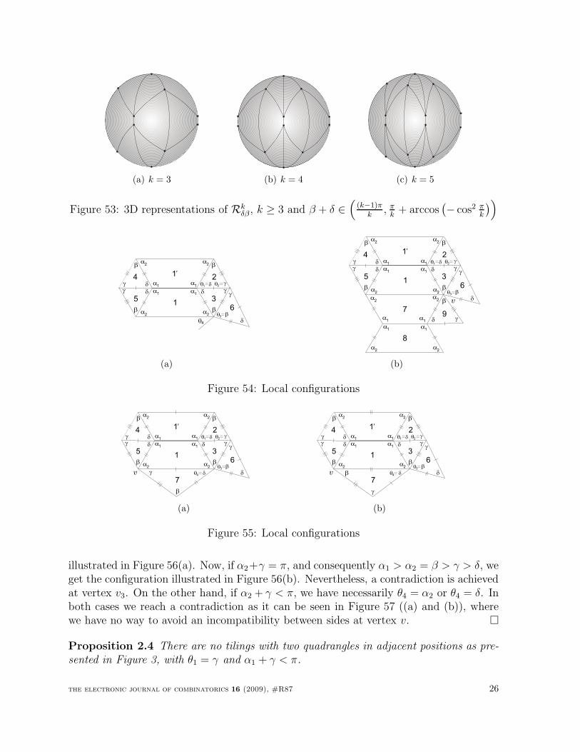
The corresponding 3D representations for 3 ≤ k ≤ 5 are illustrated in Figure 53. We de-

note such family of f-tilings by Rkδβ , with k ≥ 3 and β+δ ∈

(

(k−1)πk

, πk

+ arccos(

− cos2 πk

)

)

,

δ < πk

< β.

(ii) If α2 + β < π, then θ4 = α2 or θ4 = δ (see Figure 54(a)). In both cases we reach acontradiction, as we can observe in Figure 54(b) and Figure 55, respectively, where wehave no way to avoid an incompatibility between sides at vertex v.

2.3 If θ3 = γ (Figure 50(a)), then necessarily β + γ = π and we obtain the configuration

the electronic journal of combinatorics 16 (2009), #R87 25

(a) k = 3 (b) k = 4 (c) k = 5

Figure 53: 3D representations of Rkδβ , k ≥ 3 and β + δ ∈

(

(k−1)πk

, πk

+ arccos(

− cos2 πk

)

)

2

3

b1

1’

q

a1

a1

a2

a2

a1

a1

a2

a2

4

g

gd q2

d

q1

b

q3

6

4

5

b

gg

d

d

b

b

d

g

(a)

2

3

b1

1’

a1

a1

a2

a2

a1

a1

a2

a2

g

gd q2

d

q1

b

q3

6

4

5

b

gg

d

d

b

b

d

g

v

d9

a2

a1

a1

7

a2

8

a1

a1

a2

a2

b

g

(b)

Figure 54: Local configurations

2

3

b1

1’

a1

a1

a2

a2

a1

a1

a2

a2

g

gd q2

d

q1

b

q3

6

4

5

b

gg

d

d

b

b

d

g

v7

q4

b

g d

(a)

2

3

b1

1’

a1

a1

a2

a2

a1

a1

a2

a2

g

gd q2

d

q1

b

q3

6

4

5

b

gg

d

d

b

b

d

g

v7

q4b

g

d

(b)

Figure 55: Local configurations

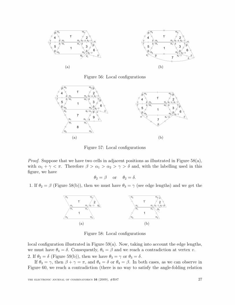
illustrated in Figure 56(a). Now, if α2+γ = π, and consequently α1 > α2 = β > γ > δ, weget the configuration illustrated in Figure 56(b). Nevertheless, a contradiction is achievedat vertex v3. On the other hand, if α2 + γ < π, we have necessarily θ4 = α2 or θ4 = δ. Inboth cases we reach a contradiction as it can be seen in Figure 57 ((a) and (b)), wherewe have no way to avoid an incompatibility between sides at vertex v.

Proposition 2.4 There are no tilings with two quadrangles in adjacent positions as pre-sented in Figure 3, with θ1 = γ and α1 + γ < π.

the electronic journal of combinatorics 16 (2009), #R87 26

2

3

b1

1’

q

a1

a1

a2

a2

a1

a1

a2

a2

4

g

gd q2

d

q1

b

q3

6

4

5

b

gg

d

d

b

d

g

v1

v2

(a)

2

3

b1

1’

a1

a1

a2

a2

a1

a1

a2

a2

g

gd q2

d

q1

b

q3

6

4

5

b

gg

d

d

b

d

g

v1

b q4g

d7v

3

(b)

Figure 56: Local configurations

2

3

b1

1’

a1

a1

a2

a2

a1

a1

a2

a2

g

gd q2

d

q1

b

q3

6

4

5

b

gg

d

d

b

g

d

b

v

d9

a2

a1

a1

7

a2

8

a1

a1

a2

a2

b

g

q4

(a)

2

3

b1

1’

a1

a1

a2

a2

a1

a1

a2

a2

g

gd q2

d

q1

b

4

5

b

gg

d

d

b

v7

q4

b

g d

q3

6g

d

b

(b)

Figure 57: Local configurations

Proof. Suppose that we have two cells in adjacent positions as illustrated in Figure 58(a),with α1 + γ < π. Therefore β > α1 > α2 > γ > δ and, with the labelling used in thisfigure, we have

θ2 = β or θ2 = δ.

1. If θ2 = β (Figure 58(b)), then we must have θ3 = γ (see edge lengths) and we get the

2

1

1’

a1

a1

a2

a2

a1

a1

a2

a2

q2q1g

(a)

2

1

1’

a1

a1

a2

a2

a1

a1

a2

a2 d

q3

bq2q1g

(b)

Figure 58: Local configurations

local configuration illustrated in Figure 59(a). Now, taking into account the edge lengths,we must have θ4 = δ. Consequently, θ5 = β and we reach a contradiction at vertex v.

2. If θ2 = δ (Figure 59(b)), then we have θ3 = γ or θ3 = δ.If θ3 = γ, then β + γ = π, and θ4 = δ or θ4 = β. In both cases, as we can observe in

Figure 60, we reach a contradiction (there is no way to satisfy the angle-folding relation

the electronic journal of combinatorics 16 (2009), #R87 27

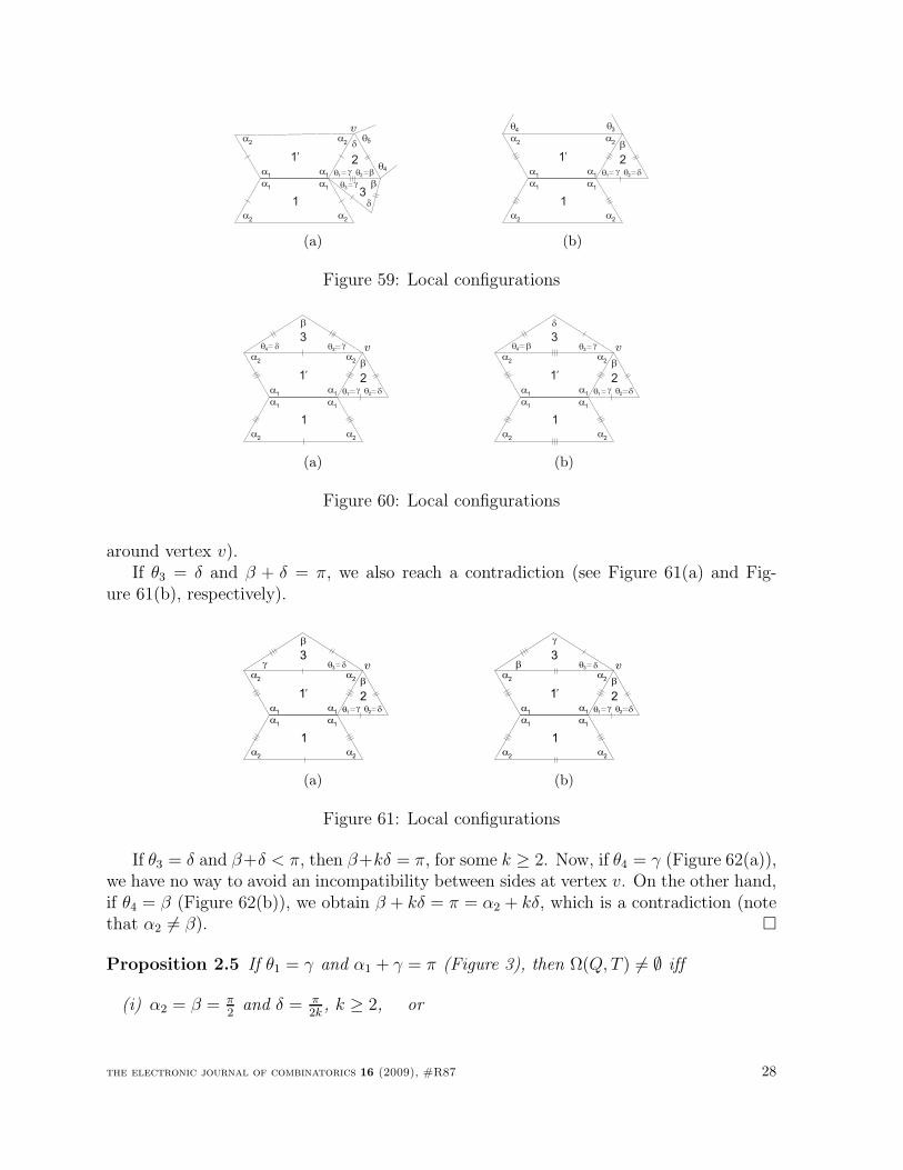
2

1

1’

a1

a1

a2

a2

a1

a1

a2

a2 d

q3g b

d3

q5

q4

v

bq2q1g

(a)

2

1

1’

a1

a1

a2

a2

a1

a1

a2

a2 b

q3q

4

dq2q1g

(b)

Figure 59: Local configurations

2

1

1’

a1

a1

a2

a2

a1

a1

a2

a2 b

q3g

3vq4 d

b

dq2q1g

(a)

2

1

1’

a1

a1

a2

a2

a1

a1

a2

a2 b

q3g

3vq4

d

b

dq2q1g

(b)

Figure 60: Local configurations

around vertex v).If θ3 = δ and β + δ = π, we also reach a contradiction (see Figure 61(a) and Fig-

ure 61(b), respectively).

2

1

1’

a1

a1

a2

a2

a1

a1

a2

a2 b

q3

3vd

b

dq2q1g

g

(a)

2

1

1’

a1

a1

a2

a2

a1

a1

a2

a2 b

q3

g

3vd

dq2q1g

b

(b)

Figure 61: Local configurations

If θ3 = δ and β+δ < π, then β+kδ = π, for some k ≥ 2. Now, if θ4 = γ (Figure 62(a)),we have no way to avoid an incompatibility between sides at vertex v. On the other hand,if θ4 = β (Figure 62(b)), we obtain β + kδ = π = α2 + kδ, which is a contradiction (notethat α2 6= β).

Proposition 2.5 If θ1 = γ and α1 + γ = π (Figure 3), then Ω(Q, T ) 6= ∅ iff

(i) α2 = β = π2

and δ = π2k

, k ≥ 2, or

the electronic journal of combinatorics 16 (2009), #R87 28

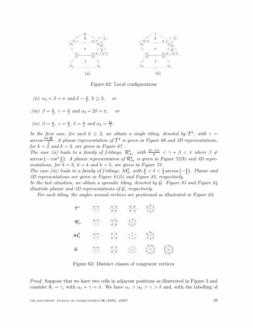
2

1

1’

a1

a1

a2

a2

a1

a1

a2

a2 b

q3g

3q4 d

b

dv

dq2q1g

(a)

2

1

1’

a1

a1

a2

a2

a1

a1

a2

a2 b

q3

g

3q4 db

dv

dq2q1g

(b)

Figure 62: Local configurations

(ii) α2 + β = π and δ = πk, k ≥ 3, or

(iii) β = π2, γ = π

3and α2 + 2δ = π, or

(iv) β = π2, γ = π

3, δ = π

5and α2 = 2π

5.

In the first case, for each k ≥ 2, we obtain a single tiling, denoted by T k, with γ =

arccossin π

2k

2. A planar representation of T k is given in Figure 66 and 3D representations,

for k = 2 and k = 3, are given in Figure 67 .The case (ii) leads to a family of f-tilings, Rk

βγ, with (k−1)πk

< γ + β < π where β 6=

arccos(

− cos2 πk

)

. A planar representation of Rkβγ is given in Figure 72(b) and 3D repre-

sentations, for k = 3, k = 4 and k = 5, are given in Figure 73.The case (iii) leads to a family of f-tilings, M3

δ, with π6

< δ < 12arccos

(

−14

)

. Planar and3D representations are given in Figure 81(b) and Figure 82, respectively.In the last situation, we obtain a sporadic tiling, denoted by G. Figure 83 and Figure 84illustrate planar and 3D representations of G, respectively.

For each tiling, the angles around vertices are positioned as illustrated in Figure 63.

Ta

2k

d

bd

ddd

d

b b

a2

bg

a1

a2

b

R

M3

G

b

dd

dd

ddd

d

d b

a2

g

a1

b b

a2

a2

g

a1

g

a1k

bgb b

a2

a2

d

d

dd

g

a1

g

a1

gg

g

g

g g

a2

d

d

dd

g

a1

g

a1

b b

b b

gg

g

g

g g

dd

dd

a2

a2

d

dd d

Figure 63: Distinct classes of congruent vertices

Proof. Suppose that we have two cells in adjacent positions as illustrated in Figure 3 andconsider θ1 = γ, with α1 + γ = π. We have α1 > α2 > γ > δ and, with the labelling of

the electronic journal of combinatorics 16 (2009), #R87 29

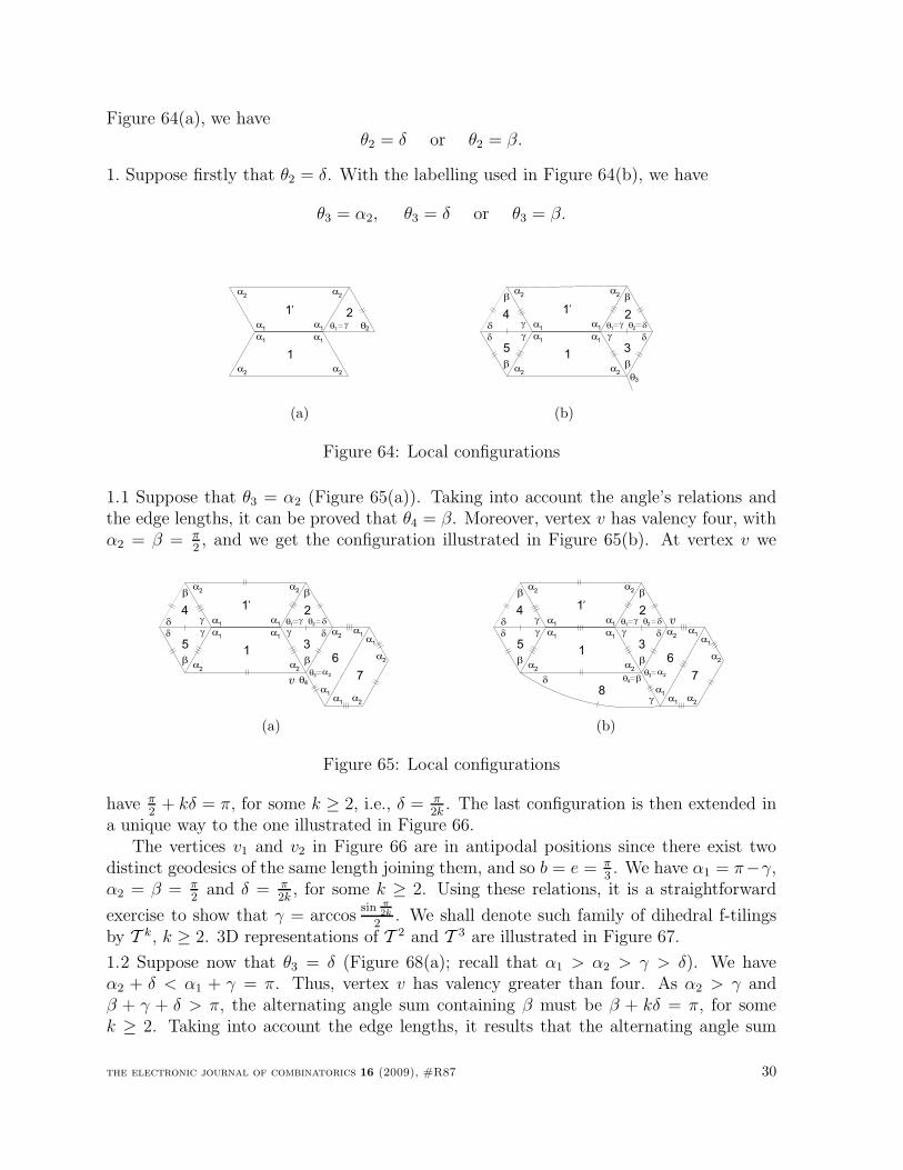
Figure 64(a), we haveθ2 = δ or θ2 = β.

1. Suppose firstly that θ2 = δ. With the labelling used in Figure 64(b), we have

θ3 = α2, θ3 = δ or θ3 = β.

2

1

1’

a1

a1

a2

a2

a1

a1

a2

a2

q2q1g

(a)

2

3

b1

1’

q

a1

a1

a2

a2

a1

a1

a2

a2

3

g

gq2

d

q1d

b

4

5

b

g

gd

d

b

(b)

Figure 64: Local configurations

1.1 Suppose that θ3 = α2 (Figure 65(a)). Taking into account the angle’s relations andthe edge lengths, it can be proved that θ4 = β. Moreover, vertex v has valency four, withα2 = β = π

2, and we get the configuration illustrated in Figure 65(b). At vertex v we

2

3

b1

1’

a1

a2

a1

a2

g

gq2

d

q1d

b

q3a

2

a1

a1

6

v

a2

a1

a2

a1

a2

4

5

b

g

gd

d

b

q4

a1

a1

7

a2

a2

(a)

2

3

b1

1’

a1

a2

a1

a2

g

gq2

d

q1d

b

q3a

2

a1

a1

6

a2

a1

a2

a1

a2

4

5

b

g

gd

d

b

8

q4

v

d b

g a1

a1

7

a2

a2

(b)

Figure 65: Local configurations

have π2

+ kδ = π, for some k ≥ 2, i.e., δ = π2k

. The last configuration is then extended ina unique way to the one illustrated in Figure 66.

The vertices v1 and v2 in Figure 66 are in antipodal positions since there exist twodistinct geodesics of the same length joining them, and so b = e = π

3. We have α1 = π−γ,

α2 = β = π2

and δ = π2k

, for some k ≥ 2. Using these relations, it is a straightforward

exercise to show that γ = arccossin π

2k

2. We shall denote such family of dihedral f-tilings

by T k, k ≥ 2. 3D representations of T 2 and T 3 are illustrated in Figure 67.

1.2 Suppose now that θ3 = δ (Figure 68(a); recall that α1 > α2 > γ > δ). We haveα2 + δ < α1 + γ = π. Thus, vertex v has valency greater than four. As α2 > γ andβ + γ + δ > π, the alternating angle sum containing β must be β + kδ = π, for somek ≥ 2. Taking into account the edge lengths, it results that the alternating angle sum

the electronic journal of combinatorics 16 (2009), #R87 30

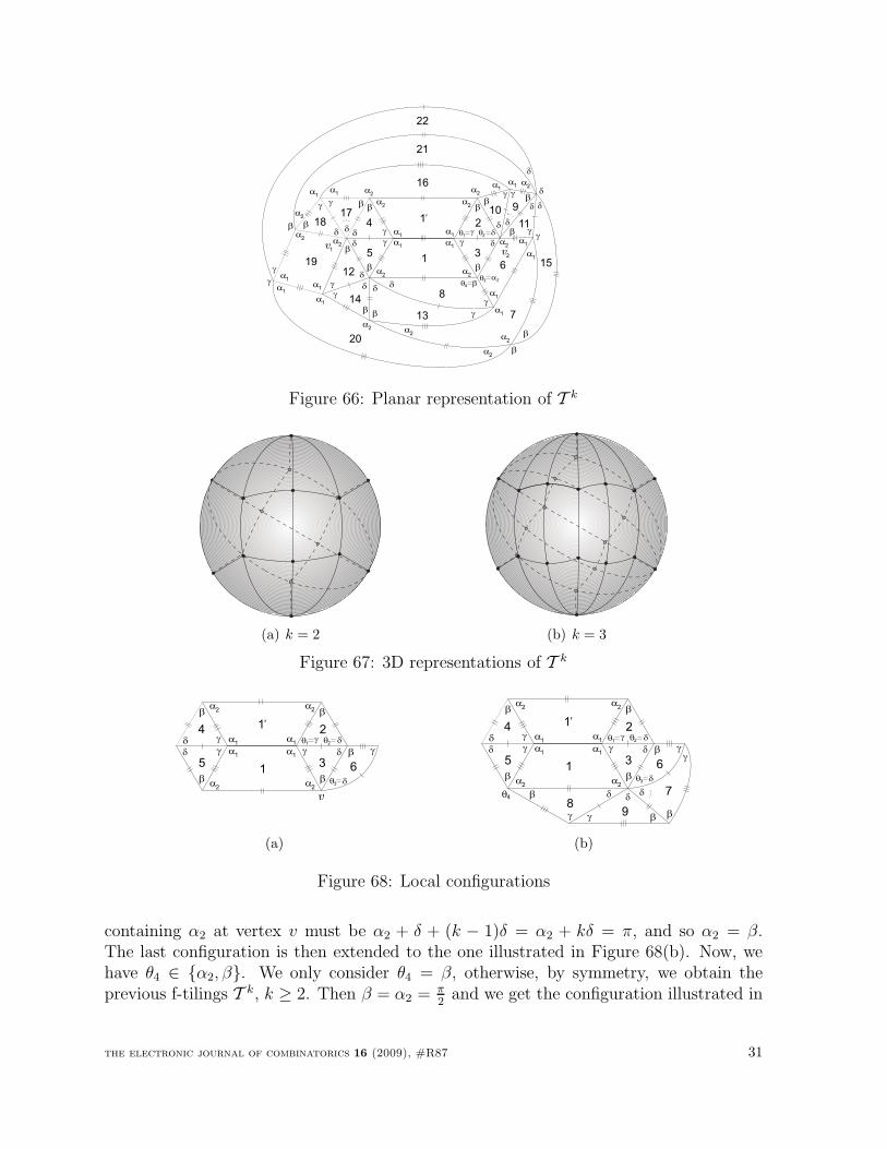
2

3

b1

1’

a1

a2

a1

a2

g

gq2

d

q1d

b

q3a

2

a1

a1

10

a2

a1

a2

a1

a2

4

5

b

g

gd

d

b

8

q4

v

d b

g

d

d d

b

b b

g

g

g13

14

12

d d

d

g

g gb b

b

6

9

11

a1

a1

a2

a2

7

g

d

b

15

dda

2

a2

b

b

gg

a1

a1

1718

19

a2

a2

a1

a1

16 a1

a1

a2

a2

21

b

g

d

22

a1

a2

a1

a2

20

b

d

g

2

v1

Figure 66: Planar representation of T k

(a) k = 2 (b) k = 3

Figure 67: 3D representations of T k

2

3

b1

1’

a1

a2

a1

a2

g

gq2

d

q1d

b

q3

6

v

a1

a2

a1

a2

4

5

b

g

gd

d

b

d

b g

(a)

2

3

b1

1’

a1

a2

a1

a2

g

gq2

d

q1d

b

q3

6

a1

a2

a1

a2

4

5

b

g

gd

d

b

d

b g

d dd

g

g g

b

b b

7

98

q4

(b)

Figure 68: Local configurations

containing α2 at vertex v must be α2 + δ + (k − 1)δ = α2 + kδ = π, and so α2 = β.The last configuration is then extended to the one illustrated in Figure 68(b). Now, wehave θ4 ∈ α2, β. We only consider θ4 = β, otherwise, by symmetry, we obtain theprevious f-tilings T k, k ≥ 2. Then β = α2 = π

2and we get the configuration illustrated in

the electronic journal of combinatorics 16 (2009), #R87 31

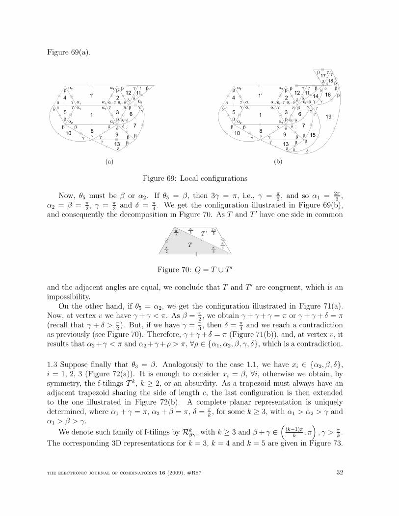
Figure 69(a).

2

3

b1

1’

a1

a2

a1

a2

g

gq2

d

q1d

b

q3

6

a1

a2

a1

a2

4

5

b

g

gd

b

d

b g

d dd

g

g g

b

b b

7

98

b

dd

g10

13

d dq5

b bg g

12 11

bg

d

(a)

2

3

b1

1’

a1

a2

a1

a2

g

gq2

d

q1d

b

q3

6

a1

a2

a1

a2

4

5

b

g

gd

b

d

b g

d dd

g

b 7

98

b

dd

g10

d d

b bg g

12 11

q5b g

d

g g b b

13bg

d

14

b

d

g

15

g

d b

16

g

b

d

19

bdd

b gg

17

18

(b)

Figure 69: Local configurations

Now, θ5 must be β or α2. If θ5 = β, then 3γ = π, i.e., γ = π3, and so α1 = 2π

3,

α2 = β = π2, γ = π

3and δ = π

4. We get the configuration illustrated in Figure 69(b),

and consequently the decomposition in Figure 70. As T and T ′ have one side in common

2p3

T

T ’p3

p3

p2

p4

p4

Figure 70: Q = T ∪ T ′

and the adjacent angles are equal, we conclude that T and T ′ are congruent, which is animpossibility.

On the other hand, if θ5 = α2, we get the configuration illustrated in Figure 71(a).Now, at vertex v we have γ + γ < π. As β = π

2, we obtain γ + γ + γ = π or γ + γ + δ = π

(recall that γ + δ > π2). But, if we have γ = π

3, then δ = π

4and we reach a contradiction

as previously (see Figure 70). Therefore, γ +γ + δ = π (Figure 71(b)), and, at vertex v, itresults that α2 +γ < π and α2 +γ+ρ > π, ∀ρ ∈ α1, α2, β, γ, δ, which is a contradiction.

1.3 Suppose finally that θ3 = β. Analogously to the case 1.1, we have xi ∈ α2, β, δ,i = 1, 2, 3 (Figure 72(a)). It is enough to consider xi = β, ∀i, otherwise we obtain, bysymmetry, the f-tilings T k, k ≥ 2, or an absurdity. As a trapezoid must always have anadjacent trapezoid sharing the side of length c, the last configuration is then extendedto the one illustrated in Figure 72(b). A complete planar representation is uniquelydetermined, where α1 + γ = π, α2 + β = π, δ = π

k, for some k ≥ 3, with α1 > α2 > γ and

α1 > β > γ.

We denote such family of f-tilings by Rkβγ , with k ≥ 3 and β + γ ∈

(

(k−1)πk

, π)

, γ > πk.

The corresponding 3D representations for k = 3, k = 4 and k = 5 are given in Figure 73.

the electronic journal of combinatorics 16 (2009), #R87 32

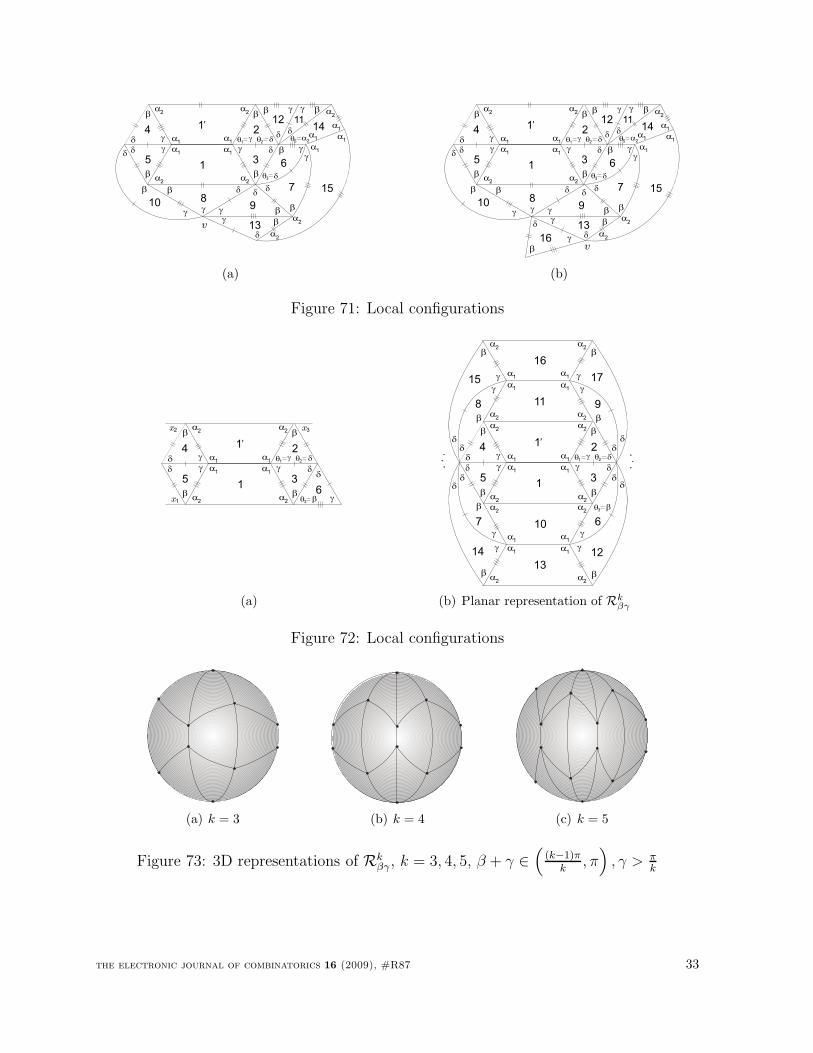
2

3

b1

1’

a1

a2

a1

a2

g

gq2

d

q1d

b

q3

6

a1

a2

a1

a2

4

5

b

g

gd

b

d

b g

d dd

g

b 7

98

b

dd

g10

d d

b bg g

12 11

g g b b

13bg

d

14

15

a2q5

a1

a1

a2

a1

a1

a2

a2

v

(a)

2

3

b1

1’

a1

a2

a1

a2

g

gq2

d

q1d

b

q3

6

a1

a2

a1

a2

4

5

b

g

gd

b

d

b g

d dd

g

b 7

98

b

dd

g10

d d

b bg g

12 11

g g b b

13bg

d

14

15

b

g

d

a2q5

a1

a1

a2

a1

a1

a2

a216

v

(b)

Figure 71: Local configurations

2

3

b1

1’

a1

a2

a1

a2

g

gq2

d

q1d

b

q3

a1

a2

a1

a2

4

5

b

g

gd

d

b

d

b gx1

6

x2 x3

(a)

2

3

b1

1’

a1

a2

a1

a2

g

gq2

d

q1d

b

q3

6

a1

a2

a1

a2

4

5

b

g

gd

d

b

d

b

g

11

a1

a2

a1

a2

10

a1

a2

a1

a2

bb

b

7

d

g

8

d

g

9

d

g

13

a1

a2

a1

a2

16

a1

a2

a1

a2

g g

g g

b b

b b

d

d

d

d

14 12

15 17

(b) Planar representation of Rkβγ

Figure 72: Local configurations

(a) k = 3 (b) k = 4 (c) k = 5

Figure 73: 3D representations of Rkβγ, k = 3, 4, 5, β + γ ∈

(

(k−1)πk

, π)

, γ > πk

the electronic journal of combinatorics 16 (2009), #R87 33

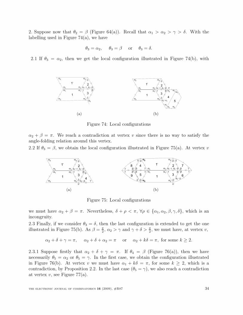
2. Suppose now that θ2 = β (Figure 64(a)). Recall that α1 > α2 > γ > δ. With thelabelling used in Figure 74(a), we have

θ3 = α2, θ3 = β or θ3 = δ.

2.1 If θ3 = α2, then we get the local configuration illustrated in Figure 74(b), with

2

3

b

1

1’

q

a1

a1

a2

a2

a1

a1

a2

a2

3

g

g

d

q2

d

q1b

(a)

2

3

b

1

1’

a1

a1

a2

a2

a1

a1

a2

a2

g

g

d

q2

d

q1b

q3a

2

a1

a1

va

2

a1

a1

a2

5

4

(b)

Figure 74: Local configurations

α2 + β = π. We reach a contradiction at vertex v since there is no way to satisfy theangle-folding relation around this vertex.

2.2 If θ3 = β, we obtain the local configuration illustrated in Figure 75(a). At vertex v

2

3

b

1

1’

a1

a1

a2

a2

a1

a1

a2

a2

g

g

d

q2

d

q1

d

q3

4

vb

b

g

(a)

1

1’

a1

a1

a2

a2

a1

a1

a2

a2

dq3

6

gb

b

d

g7

9

d

b

b

d

g8

g

a2

a2

4

5

b

g

g

d

d

b2

3

b

g

gq2

d

q1b

d

v

(b)

Figure 75: Local configurations

we must have α2 + β = π. Nevertheless, δ + ρ < π, ∀ρ ∈ α1, α2, β, γ, δ, which is anincongruity.

2.3 Finally, if we consider θ3 = δ, then the last configuration is extended to get the oneillustrated in Figure 75(b). As β = π

2, α2 > γ and γ + δ > π

2, we must have, at vertex v,

α2 + δ + γ = π, α2 + δ + α2 = π or α2 + kδ = π, for some k ≥ 2.

2.3.1 Suppose firstly that α2 + δ + γ = π. If θ4 = β (Figure 76(a)), then we havenecessarily θ5 = α2 or θ5 = γ. In the first case, we obtain the configuration illustratedin Figure 76(b). At vertex v we must have α1 + kδ = π, for some k ≥ 2, which is acontradiction, by Proposition 2.2. In the last case (θ5 = γ), we also reach a contradictionat vertex v, see Figure 77(a).

the electronic journal of combinatorics 16 (2009), #R87 34

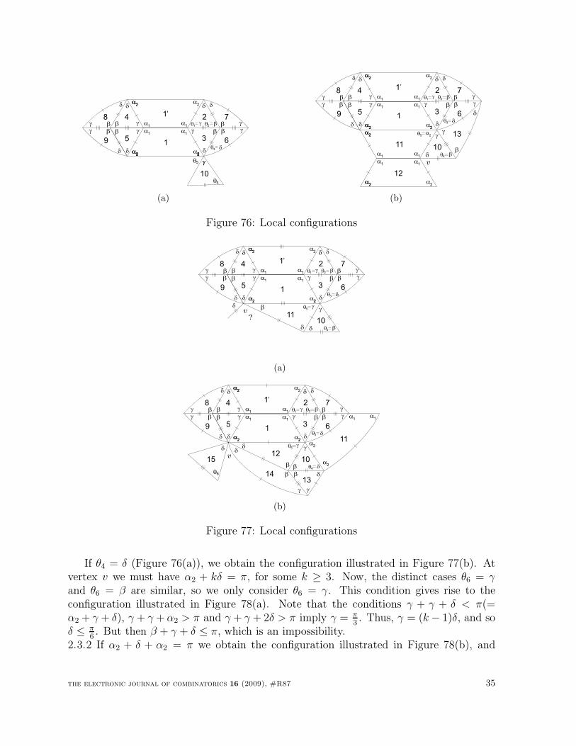
1

1’

a1

a1

a2

a2

a1

a1

a2

a2

dq3

6

gb

b

d

g7

9

d

b

b

d

g8

g

a2

a2

4

5

b

g

g

d

d

b2

3

b

g

gq2

d

q1b

d

2

g

q4

2 22 2

g

10

q5

(a)

1

1’

a1

a1

a2

a2

a1

a1

a2

a2

dq3

6

gb

b

d

g7

9

d

b

b

d

g8

g

a2

a2

4

5

b

g

g

d

d

b2

3

b

g

gq2

d

q1b

d

2

g

bq4d1011

a1

a1

a2

a2

12

a1

a1

a2

a2

a2

q5a

2

g

d

b

13

v

(b)

Figure 76: Local configurations

1

1’

a1

a1

a2

a2

a1

a1

a2

a2

dq3

6

gb

b

d

g7

9

d

b

b

d

g8

g

a2

a2

4

5

b

g

g

d

d

b2

3

b

g

gq2

d

q1b

d

2

g

bq4d10

11

q5vgb

d

?

d

(a)

1

1’

a1

a1

a2

a2

a1

a1

a2

a2

dq3

6

gb

b

d

g7

9

d

b

b

d

g8

g

a2

a2

4

5

b

g

g

d

d

b2

3

b

g

gq2

d

q1b

d

2

g

dq4

1012

q5

v

g

b

d

b

a2

a1

a1

11

g

13b db

g

d

14

15

d

q6

a2

(b)

Figure 77: Local configurations

If θ4 = δ (Figure 76(a)), we obtain the configuration illustrated in Figure 77(b). Atvertex v we must have α2 + kδ = π, for some k ≥ 3. Now, the distinct cases θ6 = γ

and θ6 = β are similar, so we only consider θ6 = γ. This condition gives rise to theconfiguration illustrated in Figure 78(a). Note that the conditions γ + γ + δ < π(=α2 + γ + δ), γ + γ + α2 > π and γ + γ + 2δ > π imply γ = π

3. Thus, γ = (k − 1)δ, and so

δ ≤ π6. But then β + γ + δ ≤ π, which is an impossibility.

2.3.2 If α2 + δ + α2 = π we obtain the configuration illustrated in Figure 78(b), and

the electronic journal of combinatorics 16 (2009), #R87 35

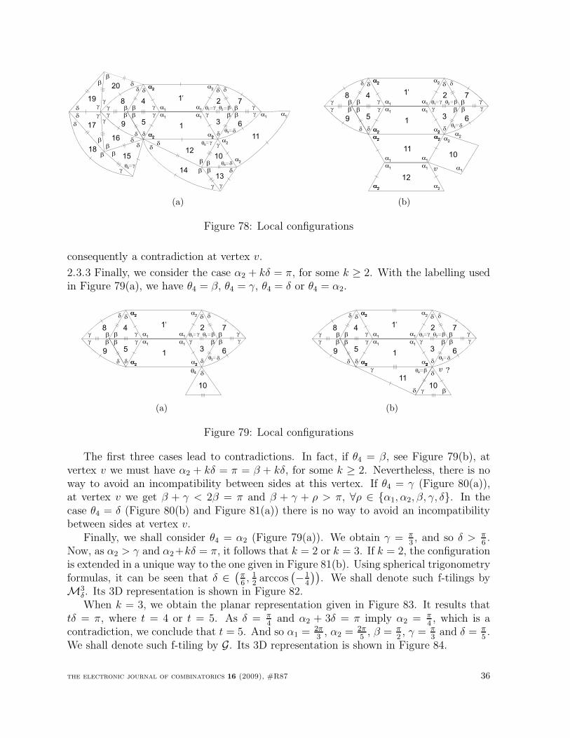
1

1’

a1

a1

a2

a2

a1

a1

a2

a2

dq3

6

gb

b

d

g7

9

d

b

b

d

g8

g

a2

a2

4

5

b

g

g

d

d

b2

3

b

g

gq2

d

q1b

d

2

g

dq4

1012

q5g

b

d

b

a2

a1

a1

11

g

13b db

g

d

14

15

d

g17

q6

g

b

b

db

g

16

d

d

b

g

18

g19

b d

b

g

20

d

a2

(a)

1

1’

a1

a1

a2

a2

a1

a1

a2

a2

dq3

6

gb

b

d

g7

9

d

b

b

d

g8

g

a2

a2

4

5

b

g

g

d

d

b2

3

b

g

gq2

d

q1b

d

2

1011

a1

a1

a2

a2

12

a1

a1

a2

a2

a2

v

a2

a2 a

2

a1

a2

(b)

Figure 78: Local configurations

consequently a contradiction at vertex v.

2.3.3 Finally, we consider the case α2 + kδ = π, for some k ≥ 2. With the labelling usedin Figure 79(a), we have θ4 = β, θ4 = γ, θ4 = δ or θ4 = α2.

1

1’

a1

a1

a2

a2

a1

a1

a2

a2

dq3

6

gb

b

d

g7

9

d

b

b

d

g8

g

a2

a2

4

5

b

g

g

d

d

b2

3

b

g

gq2

d

q1b

d

2

q4 d

10

(a)

1

1’

a1

a1

a2

a2

a1

a1

a2

a2

dq3

6

gb

b

d

g7

9

d

b

b

d

g8

g

a2

a2

4

5

b

g

g

d

d

b2

3

b

g

gq2

d

q1b

d

2

d

10

2 22 2

11

q4vbg

d g b

?

(b)

Figure 79: Local configurations

The first three cases lead to contradictions. In fact, if θ4 = β, see Figure 79(b), atvertex v we must have α2 + kδ = π = β + kδ, for some k ≥ 2. Nevertheless, there is noway to avoid an incompatibility between sides at this vertex. If θ4 = γ (Figure 80(a)),at vertex v we get β + γ < 2β = π and β + γ + ρ > π, ∀ρ ∈ α1, α2, β, γ, δ. In thecase θ4 = δ (Figure 80(b) and Figure 81(a)) there is no way to avoid an incompatibilitybetween sides at vertex v.

Finally, we shall consider θ4 = α2 (Figure 79(a)). We obtain γ = π3, and so δ > π

6.

Now, as α2 > γ and α2+kδ = π, it follows that k = 2 or k = 3. If k = 2, the configurationis extended in a unique way to the one given in Figure 81(b). Using spherical trigonometryformulas, it can be seen that δ ∈

(

π6, 1

2arccos

(

−14

))

. We shall denote such f-tilings byM3

δ. Its 3D representation is shown in Figure 82.When k = 3, we obtain the planar representation given in Figure 83. It results that

tδ = π, where t = 4 or t = 5. As δ = π4

and α2 + 3δ = π imply α2 = π4, which is a

contradiction, we conclude that t = 5. And so α1 = 2π3

, α2 = 2π5

, β = π2, γ = π

3and δ = π

5.

We shall denote such f-tiling by G. Its 3D representation is shown in Figure 84.

the electronic journal of combinatorics 16 (2009), #R87 36

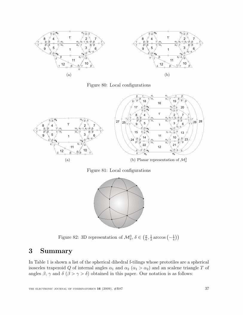
1

1’

a1

a1

a2

a2

a1

a1

a2

a2

dq3

6

gb

b

d

g7

9

d

b

b

d

g8

g

a2

a2

4

5

b

g

g

d

d

b2

3

b

g

gq2

d

q1b

d

2

d

10

2 22 2

11

q4

v

g

d g b

bd

12bg

(a)

v

1

1’

a1

a1

a2

a2

a1

a1

a2

a2

dq3

6

gb

b

d

g7

9

d

b

b

d

g8

g

a2

a2

4

5

b

g

g

d

d

b2

3

b

g

gq2

d

q1b

d

2

d

10

2 22 2

11

q4v d

g b

b

d12

b

g

g

(b)

Figure 80: Local configurations

1

1’

a1

a1

a2

a2

a1

a1

a2

a2

dq3

6

gb

b

d

g7

9

d

b

b

d

g8

g

a2

a2

4

5

b

g

g

d

d

b2

3

b

g

gq2

d

q1b

d

2

d

10

2 22 2

11

q4v d

gbbd12

b

gg

(a)

1

1’

a1

a1

a2

a2

a1

a1

a2

a2

dq3

6

gb

b

d

g7

9

d

b

b

d

g8

g

a2

a2

4

5

b

g

g

d

d

b2

3

b

g

gq2

d

q1b

d

2

11

a1

a1

a2

a2

12

a1

a1

a2

a2

a2

q4

a2 d

10g b

16

a1

a1

a2

a2

a2

d

14gb

d

18

gb

d

19

g b

dd

dd

b

b b

b

g

g

g

g

17 20

15

23

d

21

g b

d

22

gb bb

g

g

g

g

dd

13

24

b b

d d

25 26

d a2

a2

a2

a2

a1

a1g gb b

27 28

(b) Planar representation of M3

δ

Figure 81: Local configurations

Figure 82: 3D representation of M3δ, δ ∈

(

π6, 1

2arccos

(

−14

))

3 Summary

In Table 1 is shown a list of the spherical dihedral f-tilings whose prototiles are a sphericalisosceles trapezoid Q of internal angles α1 and α2 (α1 > α2) and an scalene triangle T ofangles β, γ and δ (β > γ > δ) obtained in this paper. Our notation is as follows:

the electronic journal of combinatorics 16 (2009), #R87 37

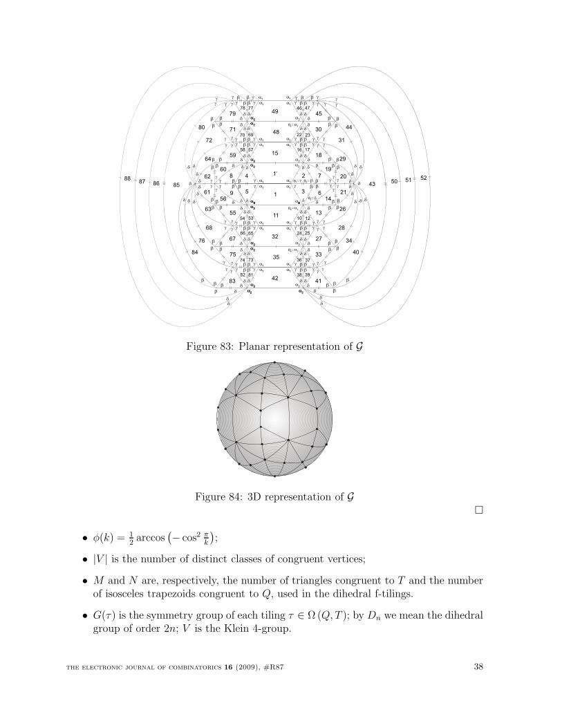
1

1’

a1

a1

a2

a2

a1

a1

a2

a2

dq3

6

gb

b

d

g7

9

d

b

b

d

g8

g

a2

a2

4

5

b

g

g

d

d

b2

3

b

g

gq2

d

q1b

d

22 22 2

11

a1

a1

a2

a2

32

a1

a1

a2

a2

a2

q4

a2

d

10g b

d

g b

b

d

g12

b

d

g

24 25

d

d

13

14

g

g

b

bd

53gb

d

gb

b

d

g54

b

d

g

6566

d

d

55

56

g

g

b

b

35

a1

a1

a2

a2

42

a1

a1

a2

a2

a2

q4

a2

d

36g b

d

g b

b

d

g37

b

d

g

38 39

d33

g

bd

73gb

d

gb

b

d

g74

b

d

g

8182

d75

g

b

g

bd27

g

b d67

49

a1

a1

a2

a2

a2

d

g b b

d

g

46 47

d

gbb

d

g

7778

48

a1

a1

a2

a2

15

a1

a1

a2

a2

a2

q4

a2

d

22g b

d

g b

b

d

g23

b

d

g

16 17

d30

g

bd

69gb

d

gb

b

d

g70

b

d

g

5758

d71

g

b

g

bd45

g

b d79

d

d

18

19

g

g

b

bd

d

59

60

g

g

b

b

g

g

b

b

d

d

21

20g

g

b

b

61

62

b

d

g

g

b

d

26

28

b

d

g

34

41

gg

d b

d

b

40

b

d

g

g

b

d

63

68

b

d

g

76

83

gg

db

d

b

84

b

d

g

g

b

d

29

31

b

d

g

44

b

d

g

g

b

d

64

72

b

d

g

80

dd

g g

b b

4385

b

d

d

g g

d d b

86 50

g b b g

dd

87 51

b g g b

d d

88 52

a1

a1

a2

a2

a2

a2

Figure 83: Planar representation of G

Figure 84: 3D representation of G

• φ(k) = 12arccos

(

− cos2 πk

)

;

• |V | is the number of distinct classes of congruent vertices;

• M and N are, respectively, the number of triangles congruent to T and the numberof isosceles trapezoids congruent to Q, used in the dihedral f-tilings.

• G(τ) is the symmetry group of each tiling τ ∈ Ω (Q, T ); by Dn we mean the dihedralgroup of order 2n; V is the Klein 4-group.

the electronic journal of combinatorics 16 (2009), #R87 38

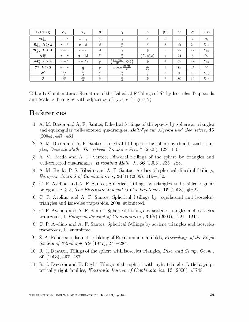
F-Tiling α1 α2 β γ δ |V | M N G(τ)

R2

δγ π − δ π − γ π

2γ δ 3 8 4 D4

Rkδβ , k ≥ 3 π − δ π − β β π

kδ 3 4k 2k D2k

Rkβγ , k ≥ 3 π − γ π − β β γ π

k3 4k 2k D2k

M3

δ π − γ π − 2δ π

2π

3

`

π

6, φ(3)

´

4 24 6 D6

Mkγ , k ≥ 4 π − δ π − 2γ π

2

“

(k−2)π2k

, φ(k)”

π

k4 8k 4k D2k

T k , k ≥ 2 π − γ π

2π

2arccos

sin π

2k

2π

2k4 8k 4k V

N 3π

5π

2π

2π

3π

55 60 10 D10

G 2π

32π

5π

2π

3π

55 80 10 D10

Table 1: Combinatorial Structure of the Dihedral F-Tilings of S2 by Isosceles Trapezoidsand Scalene Triangles with adjacency of type V (Figure 2)

References

[1] A. M. Breda and A. F. Santos, Dihedral f-tilings of the sphere by spherical trianglesand equiangular well-centered quadrangles, Beitrage zur Algebra und Geometrie, 45

(2004), 447−461.

[2] A. M. Breda and A. F. Santos, Dihedral f-tilings of the sphere by rhombi and trian-gles, Discrete Math. Theoretical Computer Sci., 7 (2005), 123−140.

[3] A. M. Breda and A. F. Santos, Dihedral f-tilings of the sphere by triangles andwell-centered quadrangles, Hiroshima Math. J., 36 (2006), 235−288.

[4] A. M. Breda, P. S. Ribeiro and A. F. Santos, A class of spherical dihedral f-tilings,European Journal of Combinatorics, 30(1) (2009), 119−132.

[5] C. P. Avelino and A. F. Santos, Spherical f-tilings by triangles and r-sided regularpolygons, r ≥ 5, The Electronic Journal of Combinatorics, 15 (2008), #R22.

[6] C. P. Avelino and A. F. Santos, Spherical f-tilings by (equilateral and isosceles)triangles and isosceles trapezoids, 2008, submitted.

[7] C. P. Avelino and A. F. Santos, Spherical f-tilings by scalene triangles and isoscelestrapezoids, I, European Journal of Combinatorics, 30(5) (2009), 1221−1244.

[8] C. P. Avelino and A. F. Santos, Spherical f-tilings by scalene triangles and isoscelestrapezoids, II, submitted.

[9] S. A. Robertson, Isometric folding of Riemannian manifolds, Proceedings of the RoyalSociety of Edinburgh, 79 (1977), 275−284.

[10] R. J. Dawson, Tilings of the sphere with isosceles triangles, Disc. and Comp. Geom.,30 (2003), 467−487.

[11] R. J. Dawson and B. Doyle, Tilings of the sphere with right triangles I: the asymp-totically right families, Electronic Journal of Combinatorics, 13 (2006), #R48.

the electronic journal of combinatorics 16 (2009), #R87 39