Spherical Arrays
35
Spherical Microphone Arrays
-
Upload
joel-pou-febles -
Category
Documents
-
view
27 -
download
3
description
Spherial Arrays, math, science, physics, arrays, polar, spherical,
Transcript of Spherical Arrays
Spherical Microphone Arrays
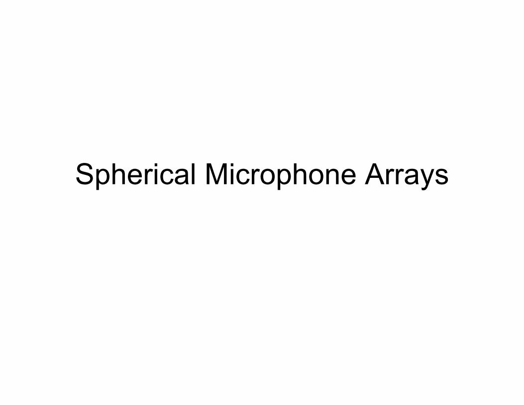
Acoustic Wave Equation
• Helmholtz Equation– Assuming the solutions of wave equation
are time harmonic waves of frequency
– satisfies the homogeneous Helmholtz equation:
ω
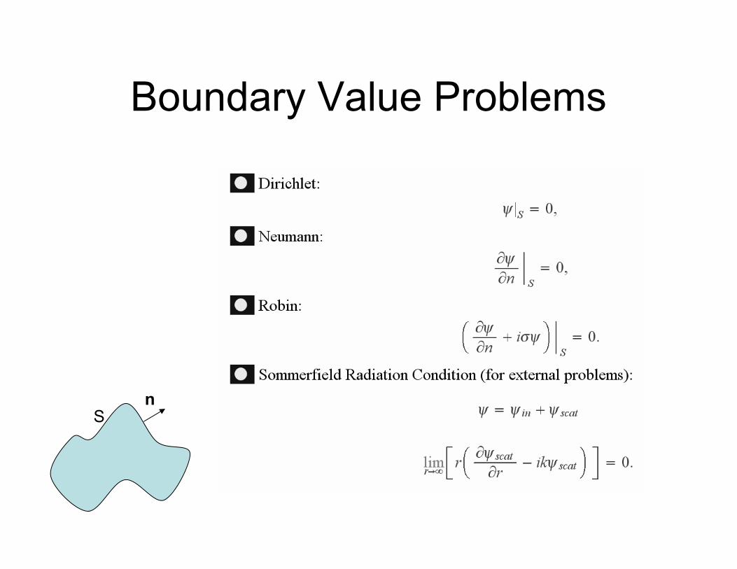
Boundary Value Problems
nS
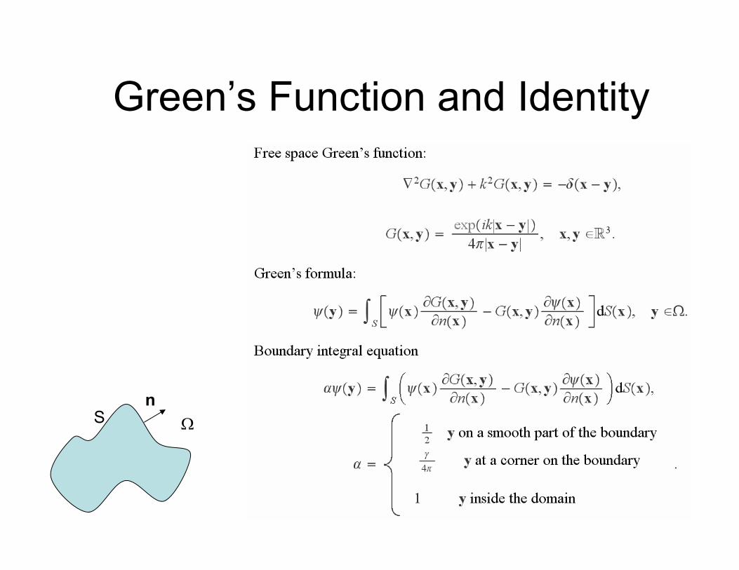
Green’s Function and Identity
nS Ω
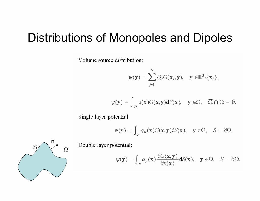
Distributions of Monopoles and Dipoles
nS Ω
Expansions in Spherical Coordinates
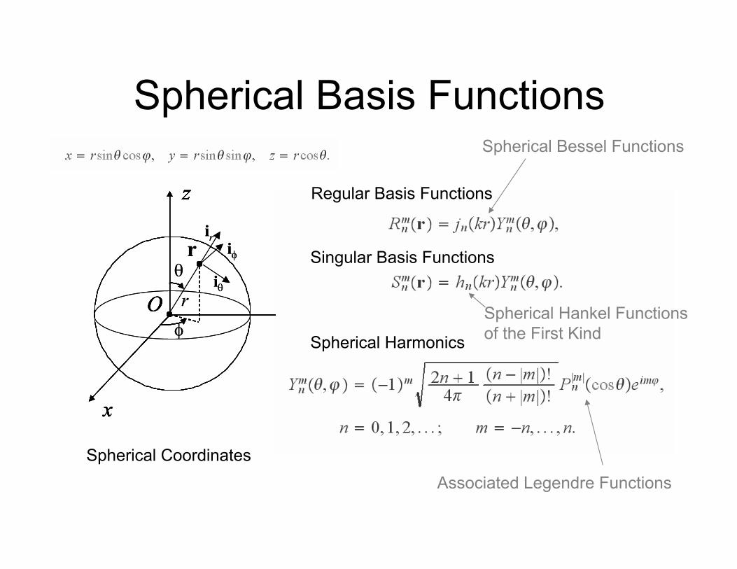
Spherical Basis Functions
x
y
z
O
x
y
z
O
x
y
z
Oθ
φ
r
rir
iθ
iφ
x
y
z
O
x
y
z
O
x
y
z
Oθ
φ
r
rir
iθ
iφ
Spherical Coordinates
Regular Basis Functions
Singular Basis Functions
Spherical Harmonics
Associated Legendre Functions
Spherical Bessel Functions
Spherical Hankel Functions of the First Kind
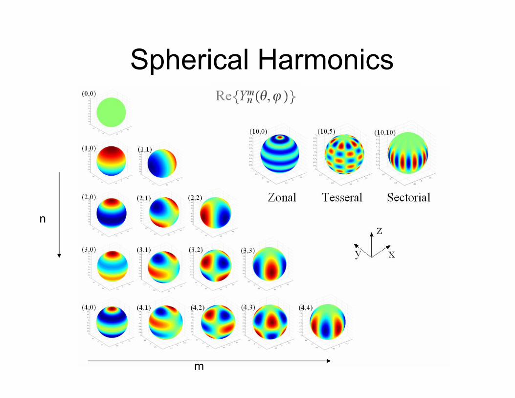
Spherical Harmonics
n
m
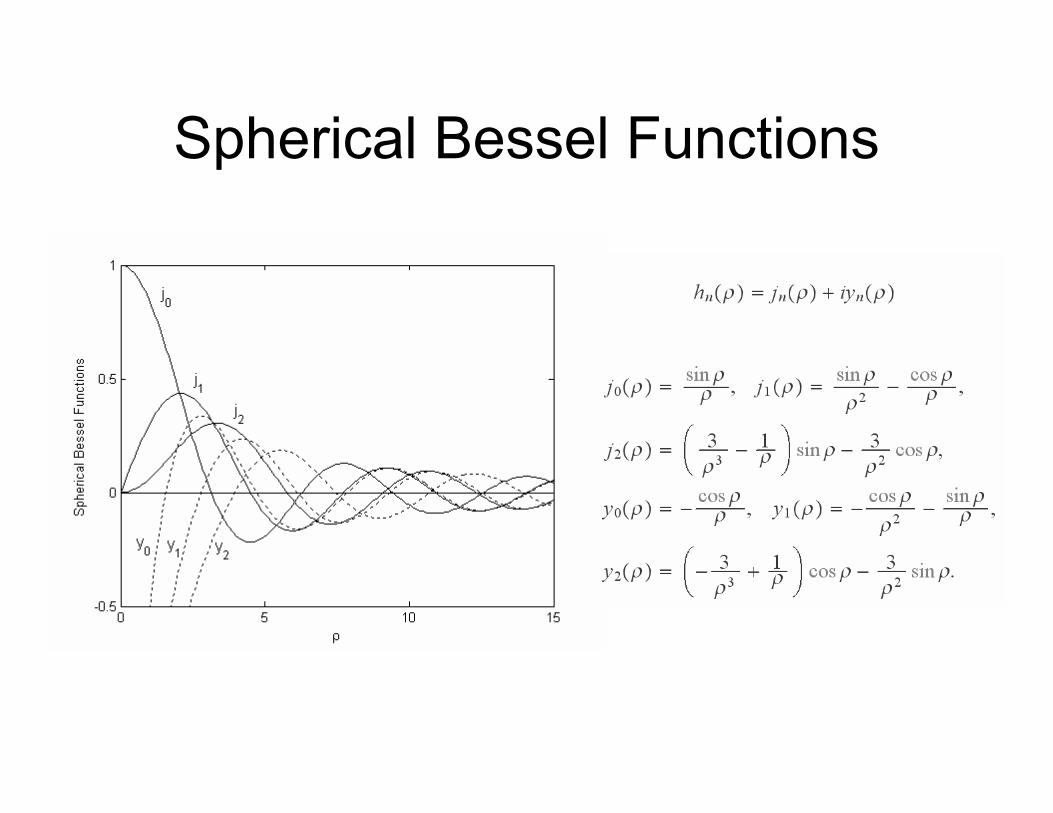
Spherical Bessel Functions
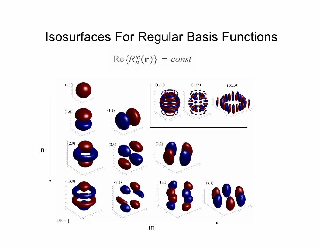
Isosurfaces For Regular Basis Functions
n
m
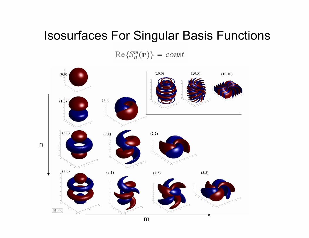
Isosurfaces For Singular Basis Functions
n
m
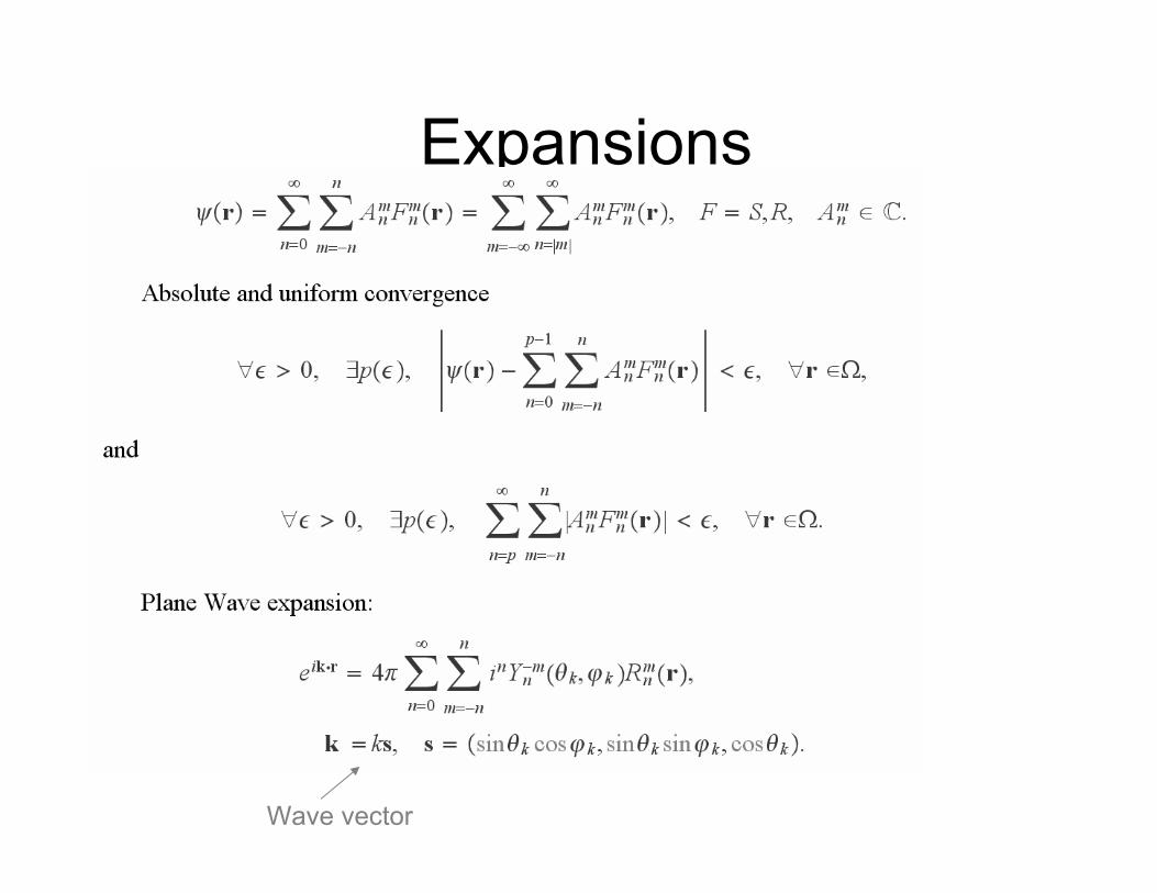
Expansions
Wave vector
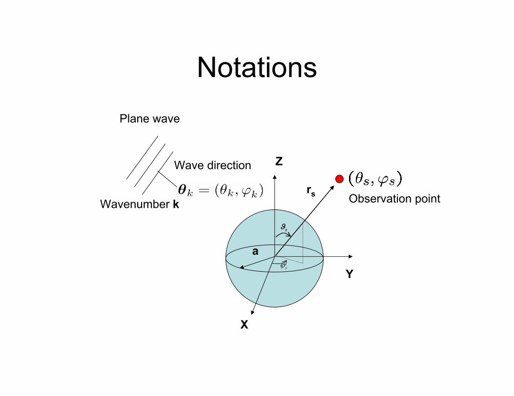
Notations
Observation point
Plane wave
Wavenumber k
Wave direction
sϕ
X
Y
a
Z
sϑ
rs
sϑ
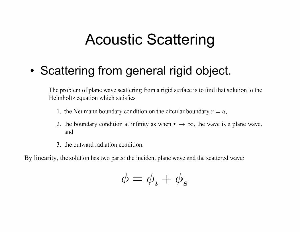
Acoustic Scattering
• Scattering from general rigid object.
By linearity, the
Acoustic Scattering
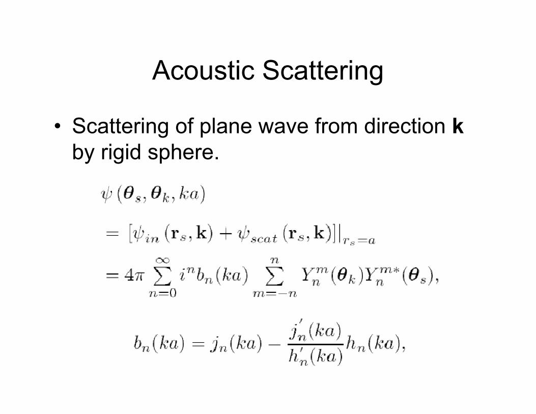
• Scattering of plane wave from direction kby rigid sphere.
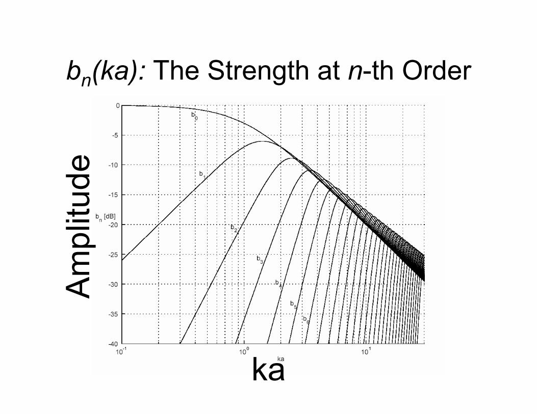
bn(ka): The Strength at n-th OrderA
mpl
itude
ka
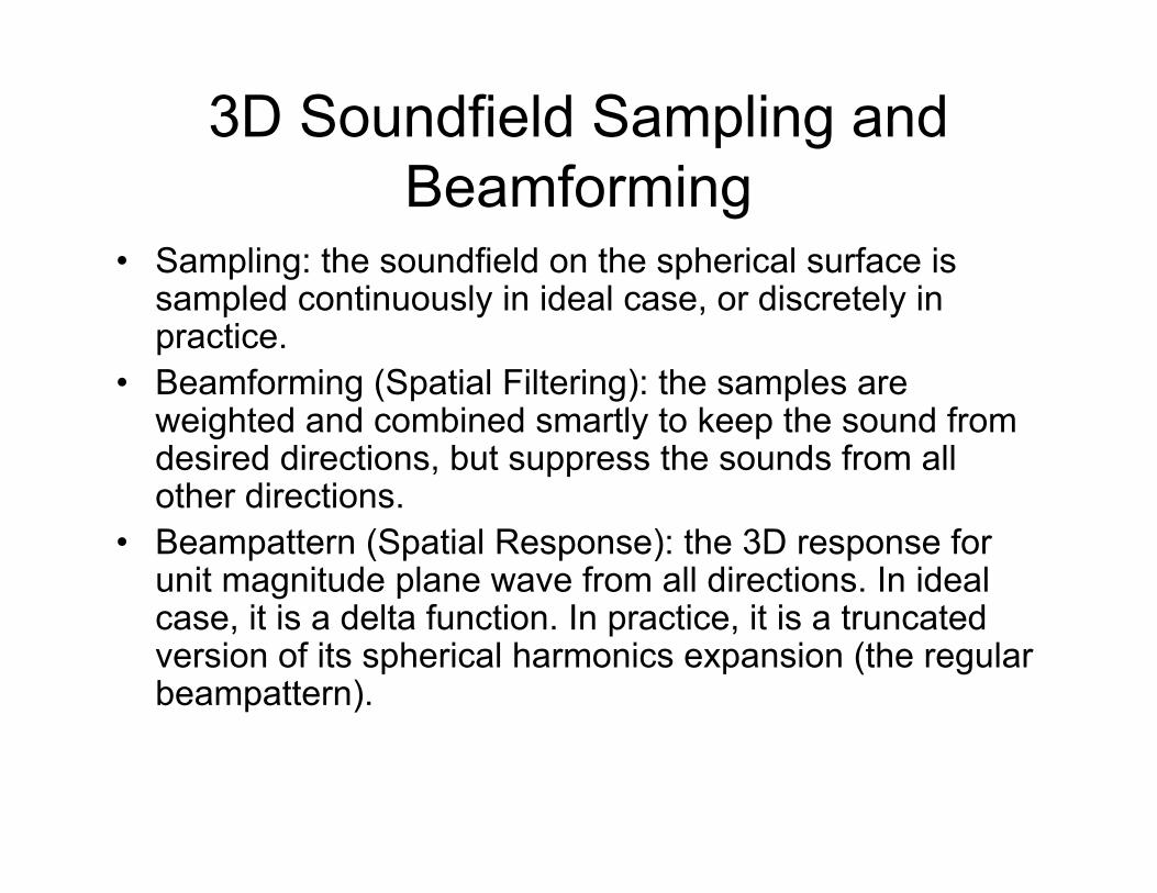
3D Soundfield Sampling and Beamforming
• Sampling: the soundfield on the spherical surface is sampled continuously in ideal case, or discretely in practice.
• Beamforming (Spatial Filtering): the samples are weighted and combined smartly to keep the sound from desired directions, but suppress the sounds from all other directions.
• Beampattern (Spatial Response): the 3D response for unit magnitude plane wave from all directions. In ideal case, it is a delta function. In practice, it is a truncated version of its spherical harmonics expansion (the regular beampattern).
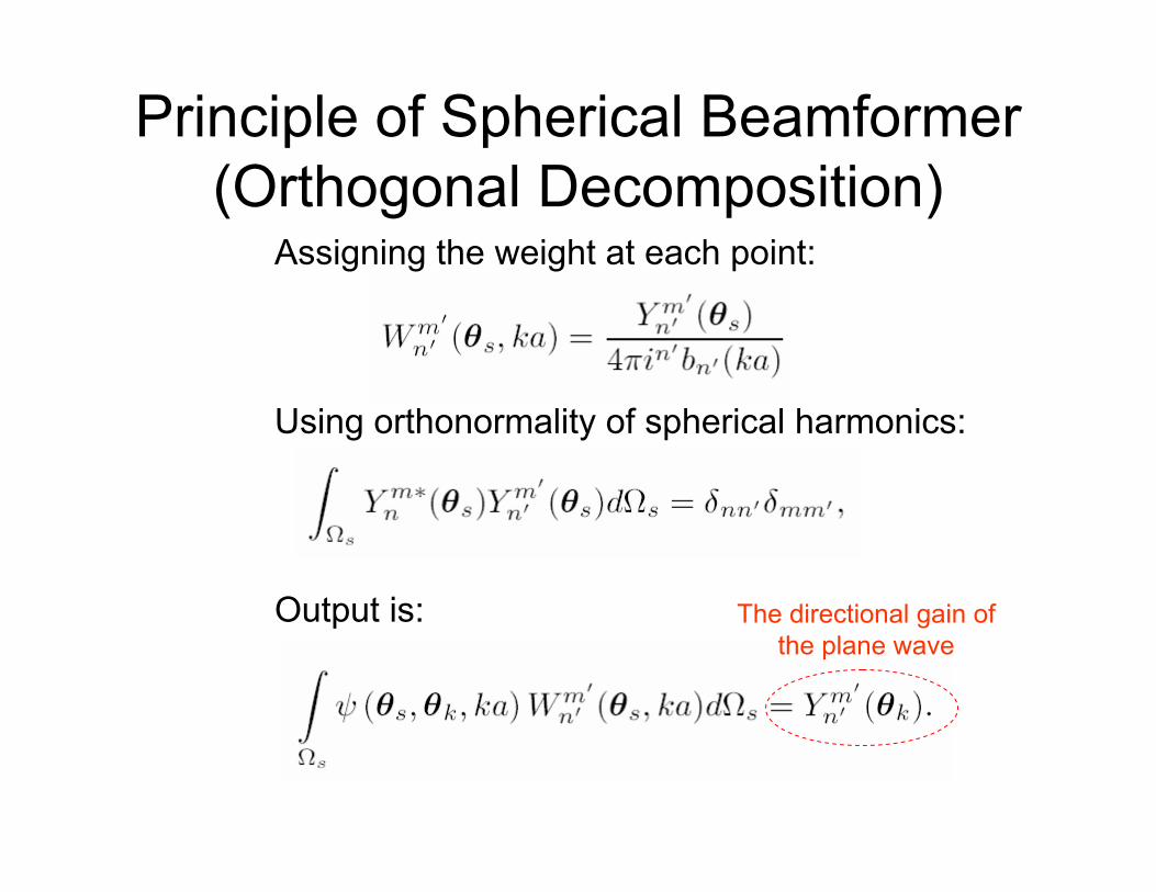
Principle of Spherical Beamformer (Orthogonal Decomposition)
Assigning the weight at each point:
Using orthonormality of spherical harmonics:
Output is: The directional gain of the plane wave
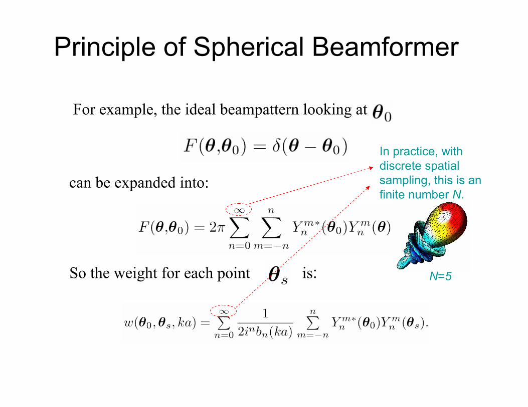
For example, the ideal beampattern looking at
Principle of Spherical Beamformer
can be expanded into:
So the weight for each point is:
In practice, with discrete spatial sampling, this is an finite number N.
N=5
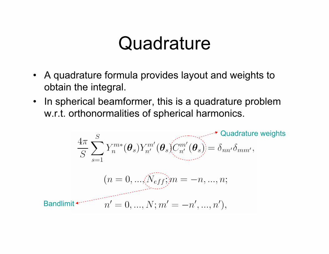
Quadrature• A quadrature formula provides layout and weights to
obtain the integral.• In spherical beamformer, this is a quadrature problem
w.r.t. orthonormalities of spherical harmonics.
Bandlimit
Quadrature weights
Quadrature Examples• Any quadrature formula of order N over the sphere
should have more than S = (N +1)2 quadrature nodes [Hardin&Sloane96][Taylor95].
• If the quadrature functions have the bandwidth up to order N, to achieve the exact quadrature using equiangular layout, we need S = 4(N + 1)2 nodes [Healy94][Healy96].
• For special layouts, S can be much smaller. For example, for a spherical grid which is a Cartesian product of equispaced grid in φ and the grid in θ in which the nodes distributed as zeros of the Legendre polynomial of degree N +1 with respect to cosθ, we need S = 2(N + 1)2 [Rafaely05].
• Spherical t-design: use special layout for equal quadrature weights. [Hardin&Sloane96]
Advantage and Disadvantage
• Advantage: – They achieve accurate quadrature results.
• Disadvantages: – They are only for strictly band-limited
functions. – S is still large considering our quadrature
function is the multiplication of two band-limited functions. This means that to achieve a beampattern of order 5 we need at least 144 microphones.
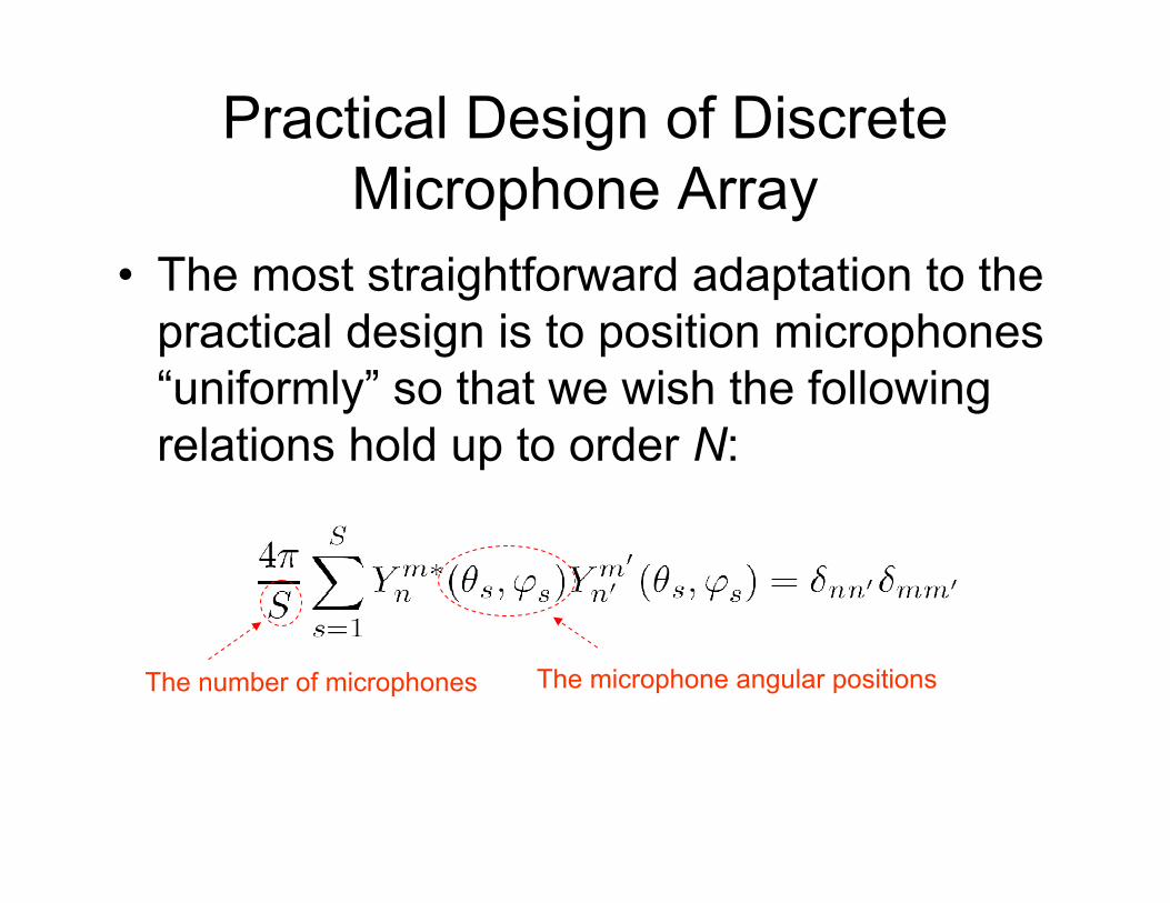
• The most straightforward adaptation to the practical design is to position microphones “uniformly” so that we wish the following relations hold up to order N:
Practical Design of Discrete Microphone Array
The number of microphones The microphone angular positions
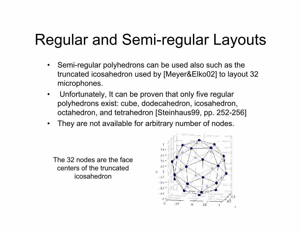
Regular and Semi-regular Layouts• Semi-regular polyhedrons can be used also such as the
truncated icosahedron used by [Meyer&Elko02] to layout 32 microphones.
• Unfortunately, It can be proven that only five regular polyhedrons exist: cube, dodecahedron, icosahedron, octahedron, and tetrahedron [Steinhaus99, pp. 252-256]
• They are not available for arbitrary number of nodes.
The 32 nodes are the face centers of the truncated
icosahedron
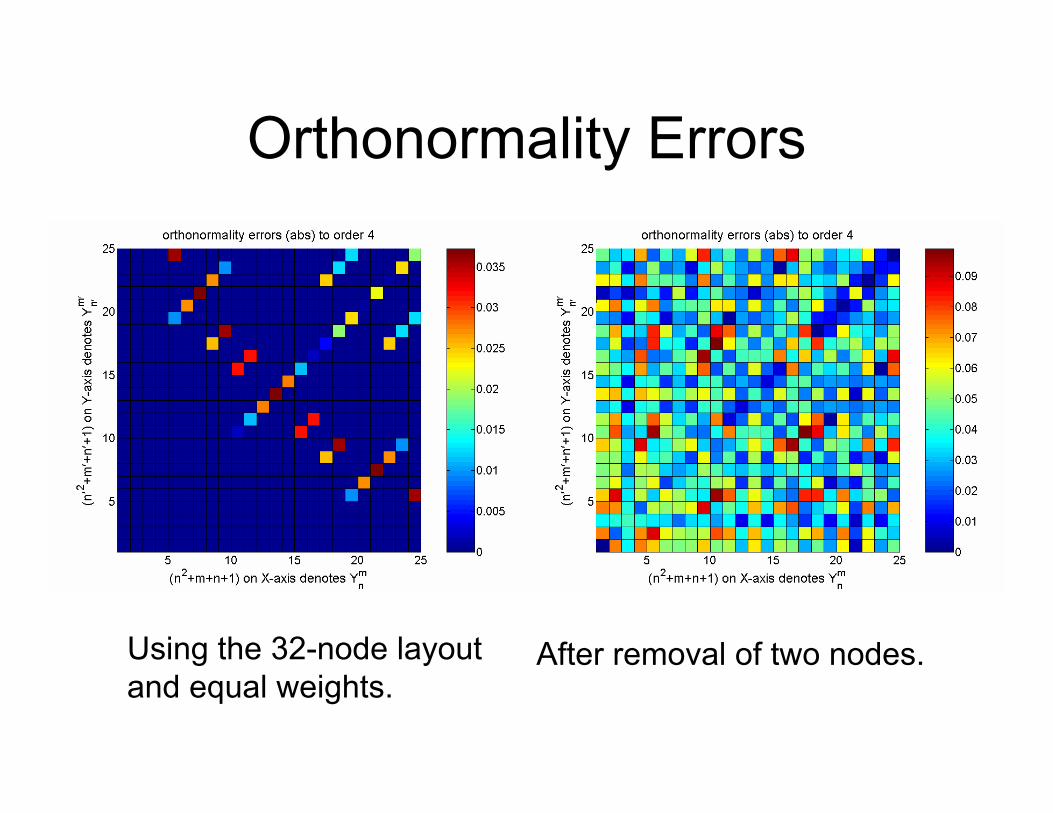
Orthonormality Errors
Using the 32-node layout and equal weights.
After removal of two nodes.
Achieve “Uniform” Layouts via Physical Simulation
• Achieve approximately “uniform” layouts for arbitrary number of nodes.
• By minimizing the potential energy of a distribution of movable electrons on a perfect conducting sphere.
• Then, one set of optimal quadrature coefficients are solved.
• [Fliege & Maier 1999].
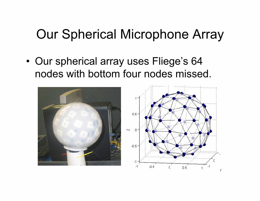
Our Spherical Microphone Array
• Our spherical array uses Fliege’s 64 nodes with bottom four nodes missed.
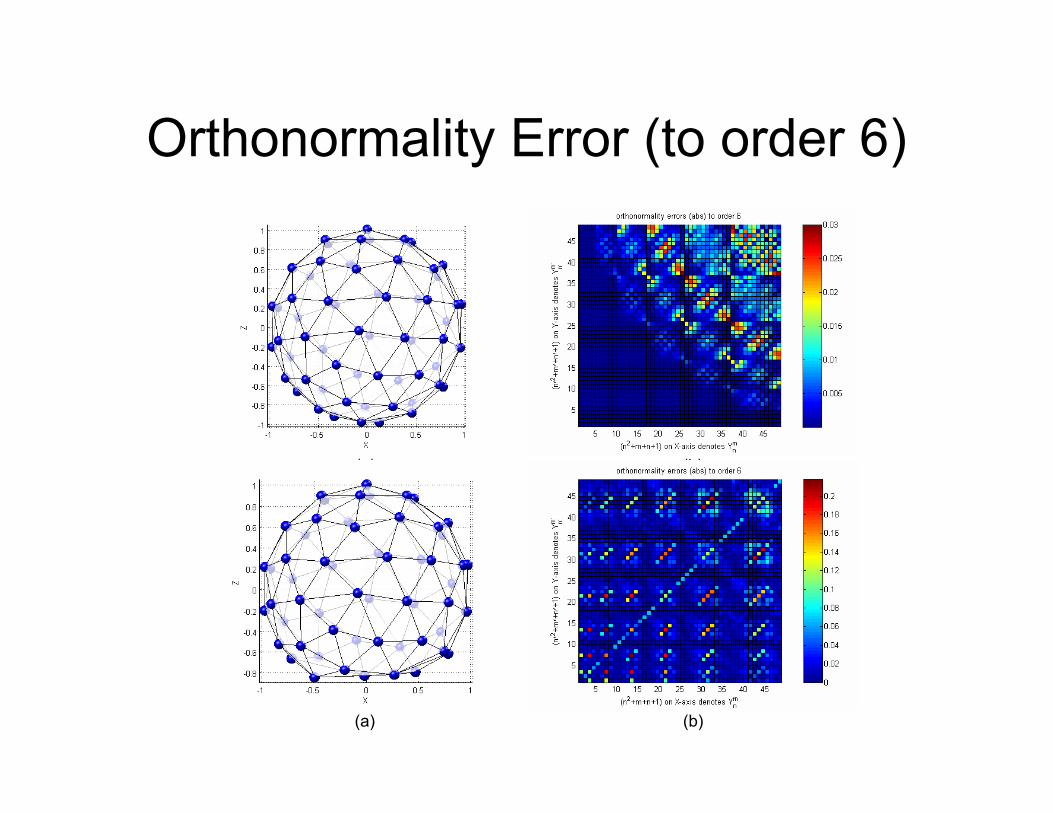
Orthonormality Error (to order 6)
(a) (b)
(a) (b)
Hemispherical Microphone Array
• In a conference table, the table surface is usually rigid and inevitably creates acoustic images.
• Given a specified number of microphones and a sphere of given radius, a hemispherical array will have a denser microphone arrangement, thereby allowing for analysis of a wider frequency range.
• Even in an acoustic environment without image sources, using a hemispherical array mounted on a rigid plane to create images may be appropriate since it provides higher order beampatterns.
• A hemispherical array is easier to build and maintain.
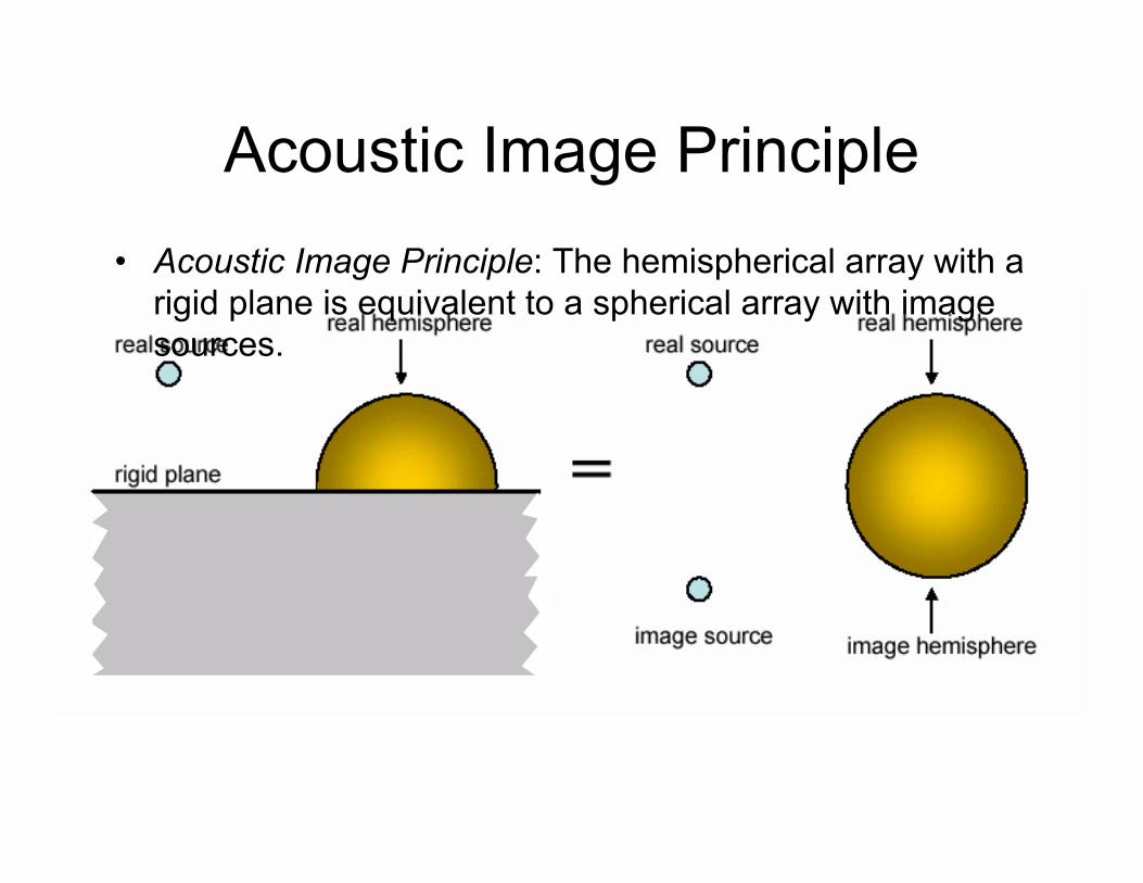
Acoustic Image Principle• Acoustic Image Principle: The hemispherical array with a
rigid plane is equivalent to a spherical array with image sources.
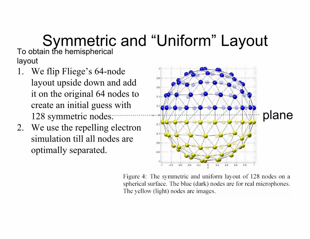
Symmetric and “Uniform” LayoutTo obtain the hemispherical layout1. We flip Fliege’s 64-node
layout upside down and add it on the original 64 nodes to create an initial guess with 128 symmetric nodes.
2. We use the repelling electron simulation till all nodes are optimally separated.
plane
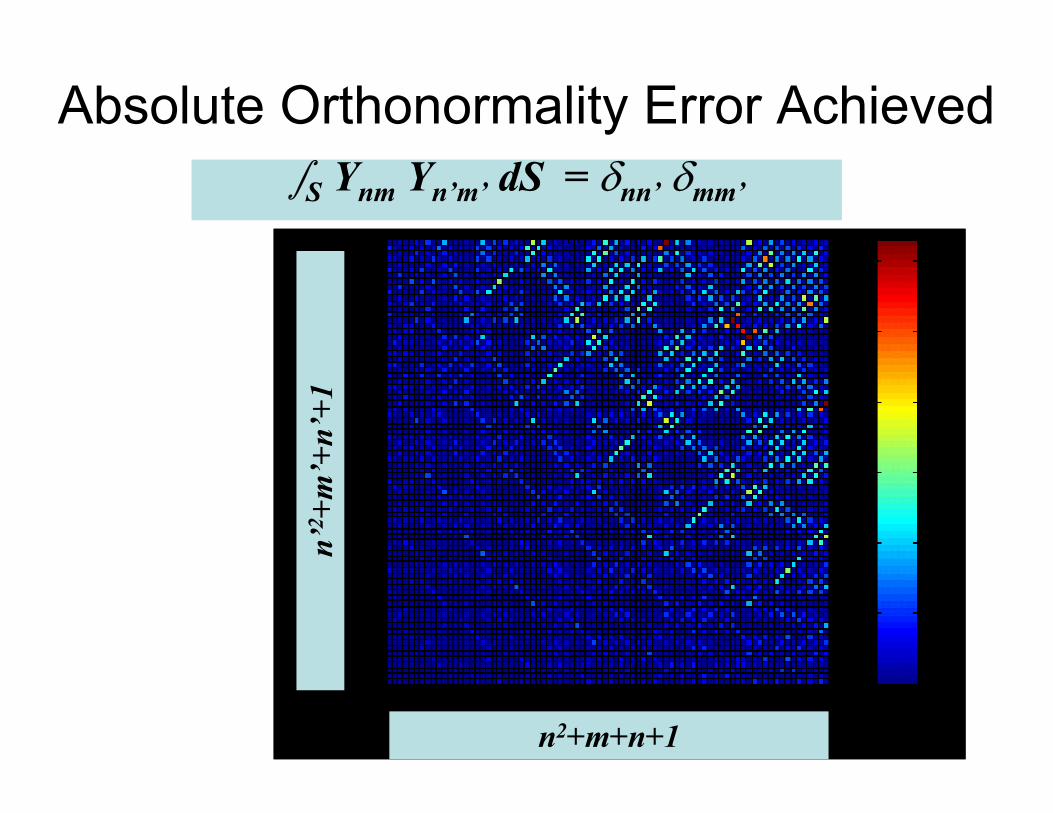
Absolute Orthonormality Error Achieved
n2+m+n+1
n’2 +
m’+
n’+1
∫S Ynm Yn’m’ dS = δnn’ δmm’
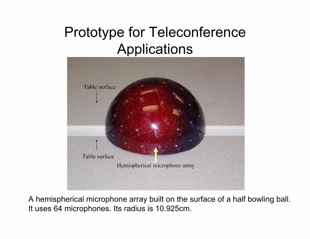
Prototype for Teleconference Applications
A hemispherical microphone array built on the surface of a half bowling ball. It uses 64 microphones. Its radius is 10.925cm.
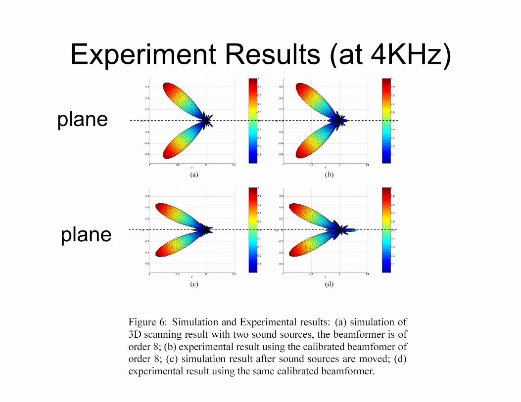
Experiment Results (at 4KHz)
plane
plane
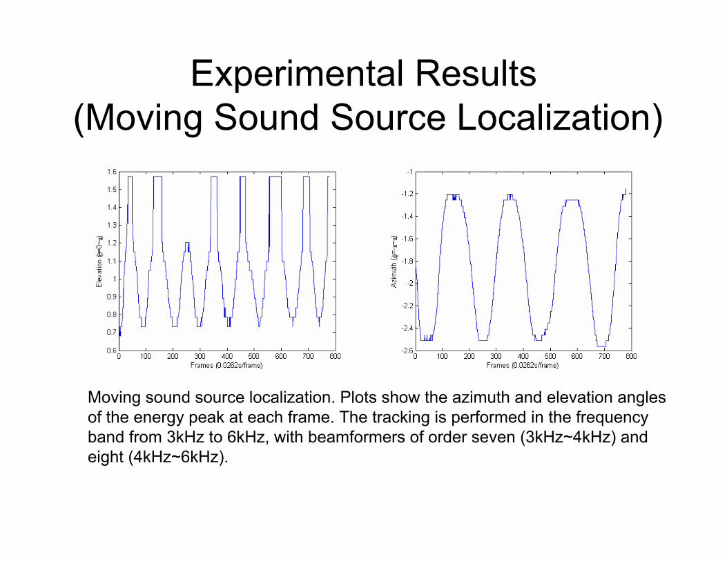
Experimental Results (Moving Sound Source Localization)
Moving sound source localization. Plots show the azimuth and elevation angles of the energy peak at each frame. The tracking is performed in the frequency band from 3kHz to 6kHz, with beamformers of order seven (3kHz~4kHz) and eight (4kHz~6kHz).


![Part III - Snvhomesnvhome.net/ee-braude/introduction2eo/figures/figures 2... · Spherical waveform coming from a real point source (after [1]). Figure 48. Gaussian-spherical wave](https://static.fdocument.org/doc/165x107/6108a4141d2cbb6d0640185d/part-iii-2-spherical-waveform-coming-from-a-real-point-source-after-1.jpg)