MATHEMATICS OF COMPUTATIONS 0025-5718(08)02128-5Article electronically published on June 24, 2008

SPECTRAL DECOMPOSITION OF REAL SYMMETRICQUADRATIC λ-MATRICES AND ITS APPLICATIONS

MOODY T. CHU AND SHU-FANG XU

Abstract. Spectral decomposition provides a canonical representation of anoperator over a vector space in terms of its eigenvalues and eigenfunctions. Thecanonical form often facilitates discussions which, otherwise, would be com-plicated and involved. Spectral decomposition is of fundamental importancein many applications. The well-known GLR theory generalizes the classicalresult of eigendecomposition to matrix polynomials of higher degrees, but itsdevelopment is based on complex numbers. This paper modifies the GLR the-ory for the special application to real symmetric quadratic matrix polynomials,Q(λ) = Mλ2 +Cλ+K, M nonsingular, subject to the specific restriction thatall matrices in the representation be real-valued. It is shown that the existenceof the real spectral decomposition can be characterized through the notion ofreal standard pair which, in turn, can be constructed from the spectral data.Applications to a variety of challenging inverse problems are discussed.

1. Introduction

Representing an operator in terms of its eigenvalues and eigenvectors, the so-called spectral decomposition, has been a powerful tool in many disciplines ofsciences and engineering. The spectral decomposition of a single matrix, oftenexpressed in the Jordan canonical form, has significant applications such as simpli-fying the representation of complicated systems, shedding light on the asymptoticbehavior of differential equations, or characterizing the performance behavior ofnumerical algorithms [13, 15]. This paper concerns itself with the spectral decom-position of a special class of quadratic λ-matrices,

(1.1) Q(λ) := Mλ2 + Cλ + K,

where M , C and K are symmetric matrices in Rn×n and M is nonsingular.

Real symmetric quadratic λ-matrices arise frequently in the study of appliedmechanics, electrical oscillation, vibro-acoustics, fluid dynamics, signal processing,and finite element model of some critical PDEs [18, 28]. The specifications ofthe underlying physical system are embedded in the matrix coefficients (M, C, K).Typically, the forward analysis involves finding scalars λ ∈ C and nonzero vectorsx ∈ Cn, called the eigenvalues and eigenvectors of the system, respectively, to satisfy

Received by the editor March 28, 2007 and, in revised form, December 12, 2007.2000 Mathematics Subject Classification. Primary 65F15, 15A22, 65F18, 93B55.Key words and phrases. Quadratic λ-matrix, spectral decomposition, real standard pair, in-

verse eigenvalue problem.Research of the first author was supported in part by the National Science Foundation under

grants DMS-0505880 and CCF-0732299.Research of the second author was supported in part by NSFC under grant 10571007.

c©2008 American Mathematical SocietyReverts to public domain 28 years from publication

1

2 MOODY T. CHU AND SHU-FANG XU

the algebraic equation Q(λ)x = 0. Our goal is to characterize a representation of thecoefficient matrices (M, C, K) in terms of the spectral data of Q(λ). The emphasisin this discussion is that all information involved in the representation must bereal-valued. The efficacy of our theory will be demonstrated by its application tosome challenging inverse problems at the end of this paper.

To motivate our consideration and set the notation for later comparison, recallfirst the classical spectral decomposition of a symmetric matrix A ∈ R

n×n,

(1.2) A = XΛX,

where X = [x1, . . . ,xn] ∈ Rn×n and Λ = diagλ1, . . . , λn ∈ R

n×n are matricescomposed of orthonormal eigenvectors xi and corresponding eigenvalues λi, re-spectively. It is important to point out that the orthogonality XX = In of theeigenvector matrix X is an intrinsic property due to the symmetry of A, which willbe explored later. Consider next the linear pencil

(1.3) L0(λ) = Bλ − A,

where A and B are symmetric matrices in Rn×n and B is positive definite. Again,

the coefficients (B, A) of the pencil can be represented as

(1.4)

B = X−X−1,A = X−ΛX−1,

where X = [x1, . . . ,xn] and Λ = diagλ1, . . . , λn, satisfying Axi = λiBxi, are stillreal matrices. It is in this sense that we call (1.4) the spectral decomposition of thelinear pencil (B, A). Note that the “orthogonality” of X is built in the first equationin (1.4) which, called B-orthogonality, can be written as XBX = In. Evenwithout the positive definiteness of B, a real symmetric pencil Bλ − A can still bereduced to the diagonal form Iλ−Λ by congruence under mild conditions such as alleigenvalues being simple, except that the nonsingular matrix X usually is complex-valued [10, 15]. (A short proof can also be found in [4] and [19, Appendix A]. Amore complete and systematic development is made in [23].) If the transformationis limited to real congruence, then the diagonal form should be replaced by a blockdiagonal form with at most 2 × 2 blocks along the diagonal [12, Theorem 1.5.4].See also [24] for a different scenario, where B is real symmetric and A is real skew-symmetric. In this paper we ask whether a similar notion can be generalized to thereal symmetric quadratic λ-matrix Q(λ) where three coefficient matrices (M, C, K)are to be decomposed simultaneously.

The query we are asking is a classical problem already considered in the seminalbook by Gohberg, Lancaster and Rodman [11]. Indeed, via the notion of Jordantriple the GLR theory developed in [11] works for general matrix polynomials ofarbitrary degrees. If the coefficients of the matrix polynomial are self-adjoint, thenadditional properties such as the existence of a self-adjoint triple and the signcharacteristic can be developed from the theory [11, Chapter 10]. As an example, wemention a case studied in [22] for a real symmetric quadratic λ-matrix Q(λ) underthe assumption that all eigenvalues are simple and nonreal. Let Xc = [x1, . . . ,xn]and Λ = diagλ1, . . . , λn denote n × n matrices of (half of) the eigenvectors andthe eigenvalues, respectively, where λi are those eigenvalues residing in the upper

SPECTRAL DECOMPOSITION FOR QUADRATIC MATRIX POLYNOMIALS 3

half-complex plane. Define

X := [Xc, Xc] ∈ Cn×2n,(1.5)

T :=[

Λ 00 Λ

]∈ C

2n×2n.(1.6)

The GLR theory [22, Theorem 2] asserts that if the matrix

(1.7) U :=[

XX T

]∈ C

2n×2n

is nonsingular (so that (X , T ) forms a complex Jordan pair), then the eigenvectormatrix X enjoys the “orthogonality”,

(1.8) X X = 0,

and the matrix coefficients (M, C, K) can be decomposed as

(1.9)

⎧⎨⎩M = (X T X )−1,C = −M(X T 2X )M,K = −(X T −1X )−1.

The challenge is that, even with symmetry, a real symmetric matrix polynomialoften has complex-valued eigenstructure [10]. The Jordan pair (X , T ) constructedabove by the GLR theory for the spectral decomposition (1.9) is complex-valued.A real-valued decomposition for the real coefficients of a quadratic λ-matrix in thesame spirit of (1.4) for a linear pencil is not obvious. One of our contributions isto fill in the details of a real-valued spectral decomposition. Additionally, we showthat the real-valued spectral decomposition of Q(λ) naturally carries a speciallystructured scaling factor which we could consider as a “parameter”. Its simplestform helps to facilitate the study of some inverse problems. Our main thrust inthis paper is to investigate these properties and to demonstrate some interestingapplications.

2. Spectral Decomposition

Linearization is a rather convenient way to cast a matrix polynomial as a linearproblem [14]. One special way to linearize the real symmetric quadratic λ-matrixQ(λ) is the linear pencil,

(2.1) L(λ) := L(λ; M, C, K) =[

C MM 0

]λ −

[−K 00 M

].

It is easy to see that Q(λ) and L(λ) are equivalent in the sense that Q(λ)x = 0 ifand only if

(2.2)([

C MM 0

]λ −

[−K 00 M

]) [xy

]= 0.

Because we have assumed that M is nonsingular, we even know that y = λx.Clearly, L(λ) is real symmetric. Note, however, that the leading coefficient [ C M

M 0 ]of L(λ) is not positive definite, so the decomposition for Q(λ) cannot be answereddirectly in the same way as the decomposition (1.4) for L0(λ).

At present, we have not yet assumed any eigenstructure of Q(λ). It is entirelypossible that the eigenvalues are complex-valued or have high geometric multiplic-ities. The notion of standard pair introduced in [11] will be a fundamental toolfor our development. The canonical form of a standard pair can be considered as

4 MOODY T. CHU AND SHU-FANG XU

a generalization of the Jordan canonical form to matrix polynomials. So that thispaper is self-contained, we briefly review the ideas below, but limit ourselves to thespecial class of real symmetric quadratic polynomials (1.1) and require specificallythat all matrices involved be real-valued. From time to time, we shall compareour real formulation with its counterpart of complex formulation already developedin [11] and point out the difference when the demand for real-valued matrices isenforced.

The symmetry of the matrix coefficients is not essential in the following definitionbut we insist that M must be nonsingular.

Definition 2.1. A pair of matrices (X, T) ∈ Rn×2n × R2n×2n is called a realstandard pair for the quadratic λ-matrix Q(λ) if and only if the matrix

(2.3) U = U(X, T) :=[

X

XT

]is nonsingular and the equation

(2.4) MXT2 + CXT + KX = 0

holds.

The existence of a real standard pair for Q(λ) is clear. Direct computation showsthat the special choice (X0, T0) with

(2.5)

⎧⎨⎩X0 := [In, 0],

T0 :=[

0 I−M−1K −M−1C

],

is a real standard pair of Q(λ). The problem is that the self-reference of (X0, T0)to the original matrix coefficients makes this pair not very useful in practice. Weseek real standard pairs that contain the eigeninformation more explicitly. We shallconstruct such a real standard pair later, but first we point out the following resultthat shows how two arbitrary real standard pairs are related to each other. Theproof follows directly from [11, Theorem 1.25].

Lemma 2.2. Let (X1, T1) be a given real standard pair of Q(λ). Then (X2, T2) isalso a real standard pair of Q(λ) if and only if

(2.6)

X2 = X1S,T2 = S−1T1S,

for some 2n × 2n real invertible matrix S. In this case, S is uniquely determinedby

(2.7) S :=[

X1

X1T1

]−1 [X2

X2T2

].

Rewriting (2.4) as

(2.8)[

C MM 0

] [X

XT

]T =

[−K 00 M

] [X

XT

],

we see that

L(λ)U =[

C MM 0

]U(λI − T).

SPECTRAL DECOMPOSITION FOR QUADRATIC MATRIX POLYNOMIALS 5

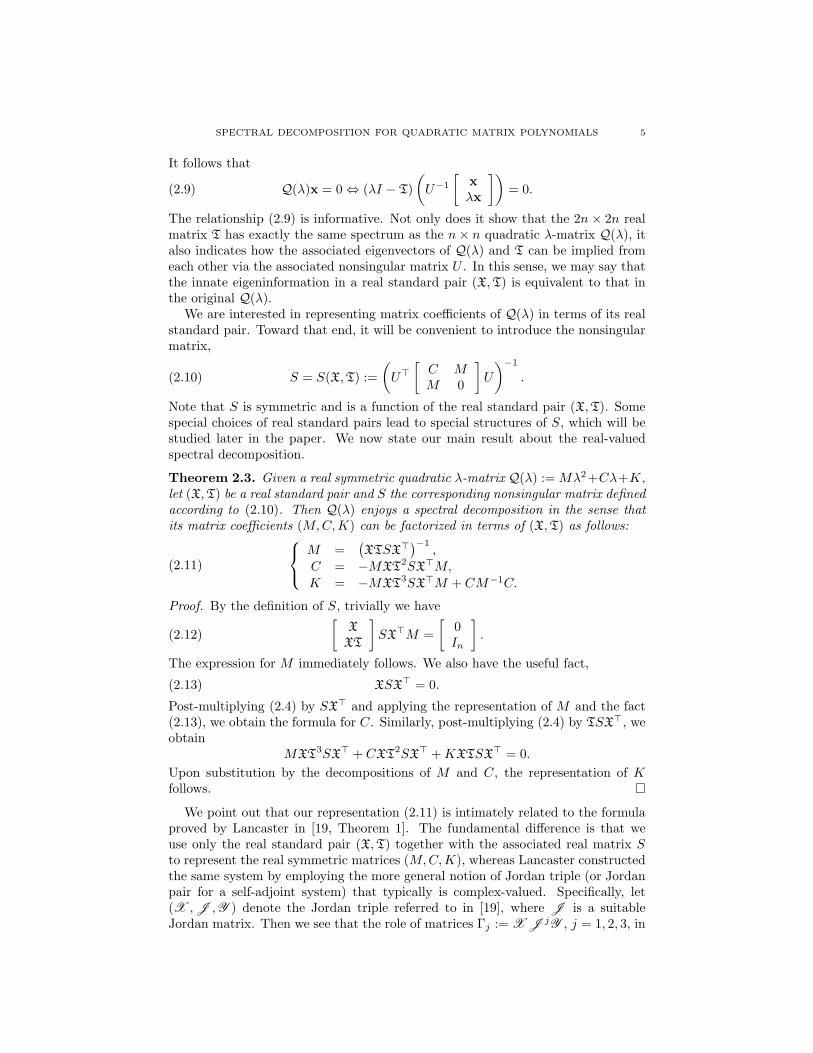
It follows that

(2.9) Q(λ)x = 0 ⇔ (λI − T)(

U−1

[xλx

])= 0.

The relationship (2.9) is informative. Not only does it show that the 2n × 2n realmatrix T has exactly the same spectrum as the n × n quadratic λ-matrix Q(λ), italso indicates how the associated eigenvectors of Q(λ) and T can be implied fromeach other via the associated nonsingular matrix U . In this sense, we may say thatthe innate eigeninformation in a real standard pair (X, T) is equivalent to that inthe original Q(λ).

We are interested in representing matrix coefficients of Q(λ) in terms of its realstandard pair. Toward that end, it will be convenient to introduce the nonsingularmatrix,

(2.10) S = S(X, T) :=(

U[

C MM 0

]U

)−1

.

Note that S is symmetric and is a function of the real standard pair (X, T). Somespecial choices of real standard pairs lead to special structures of S, which will bestudied later in the paper. We now state our main result about the real-valuedspectral decomposition.

Theorem 2.3. Given a real symmetric quadratic λ-matrix Q(λ) := Mλ2+Cλ+K,let (X, T) be a real standard pair and S the corresponding nonsingular matrix definedaccording to (2.10). Then Q(λ) enjoys a spectral decomposition in the sense thatits matrix coefficients (M, C, K) can be factorized in terms of (X, T) as follows:

(2.11)

⎧⎨⎩ M =(XTSX)−1

,

C = −MXT2SXM,

K = −MXT3SXM + CM−1C.

Proof. By the definition of S, trivially we have

(2.12)[

X

XT

]SX

M =[

0In

].

The expression for M immediately follows. We also have the useful fact,

(2.13) XSX = 0.

Post-multiplying (2.4) by SX and applying the representation of M and the fact(2.13), we obtain the formula for C. Similarly, post-multiplying (2.4) by TSX, weobtain

MXT3SX

+ CXT2SX

+ KXTSX = 0.

Upon substitution by the decompositions of M and C, the representation of Kfollows.

We point out that our representation (2.11) is intimately related to the formulaproved by Lancaster in [19, Theorem 1]. The fundamental difference is that weuse only the real standard pair (X, T) together with the associated real matrix Sto represent the real symmetric matrices (M, C, K), whereas Lancaster constructedthe same system by employing the more general notion of Jordan triple (or Jordanpair for a self-adjoint system) that typically is complex-valued. Specifically, let(X , J , Y ) denote the Jordan triple referred to in [19], where J is a suitableJordan matrix. Then we see that the role of matrices Γj := X J jY , j = 1, 2, 3, in

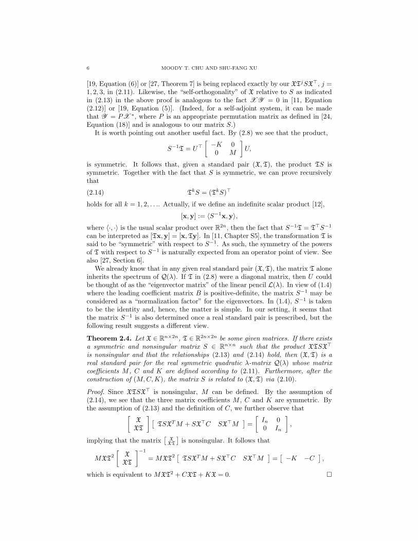
6 MOODY T. CHU AND SHU-FANG XU

[19, Equation (6)] or [27, Theorem 7] is being replaced exactly by our XTjSX, j =1, 2, 3, in (2.11). Likewise, the “self-orthogonality” of X relative to S as indicatedin (2.13) in the above proof is analogous to the fact X Y = 0 in [11, Equation(2.12)] or [19, Equation (5)]. (Indeed, for a self-adjoint system, it can be madethat Y = PX ∗, where P is an appropriate permutation matrix as defined in [24,Equation (18)] and is analogous to our matrix S.)

It is worth pointing out another useful fact. By (2.8) we see that the product,

S−1T = U

[−K 00 M

]U,

is symmetric. It follows that, given a standard pair (X, T), the product TS issymmetric. Together with the fact that S is symmetric, we can prove recursivelythat

(2.14) TkS = (TkS)

holds for all k = 1, 2, . . .. Actually, if we define an indefinite scalar product [12],

[x,y] := 〈S−1x,y〉,where 〈·, ·〉 is the usual scalar product over R

2n, then the fact that S−1T = TS−1

can be interpreted as [Tx,y] = [x, Ty]. In [11, Chapter S5], the transformation T issaid to be “symmetric” with respect to S−1. As such, the symmetry of the powersof T with respect to S−1 is naturally expected from an operator point of view. Seealso [27, Section 6].

We already know that in any given real standard pair (X, T), the matrix T aloneinherits the spectrum of Q(λ). If T in (2.8) were a diagonal matrix, then U couldbe thought of as the “eigenvector matrix” of the linear pencil L(λ). In view of (1.4)where the leading coefficient matrix B is positive-definite, the matrix S−1 may beconsidered as a “normalization factor” for the eigenvectors. In (1.4), S−1 is takento be the identity and, hence, the matter is simple. In our setting, it seems thatthe matrix S−1 is also determined once a real standard pair is prescribed, but thefollowing result suggests a different view.

Theorem 2.4. Let X ∈ Rn×2n, T ∈ R2n×2n be some given matrices. If there existsa symmetric and nonsingular matrix S ∈ Rn×n such that the product XTSX

is nonsingular and that the relationships (2.13) and (2.14) hold, then (X, T) is areal standard pair for the real symmetric quadratic λ-matrix Q(λ) whose matrixcoefficients M , C and K are defined according to (2.11). Furthermore, after theconstruction of (M, C, K), the matrix S is related to (X, T) via (2.10).

Proof. Since XTSX is nonsingular, M can be defined. By the assumption of(2.14), we see that the three matrix coefficients M , C and K are symmetric. Bythe assumption of (2.13) and the definition of C, we further observe that[

X

XT

] [TSXT M + SXC SXM

]=

[In 00 In

],

implying that the matrix[

XXT

]is nonsingular. It follows that

MXT2

[X

XT

]−1

= MXT2[

TSXT M + SXC SXM]

=[−K −C

],

which is equivalent to MXT2 + CXT + KX = 0.

SPECTRAL DECOMPOSITION FOR QUADRATIC MATRIX POLYNOMIALS 7

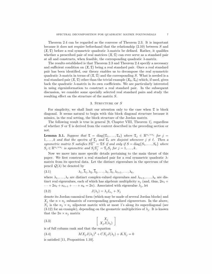
Theorem 2.4 can be regarded as the converse of Theorem 2.3. It is importantbecause it does not require beforehand that the relationship (2.10) between S and(X, T) before a real symmetric quadratic λ-matrix be defined. Rather, it qualifieswhether a prescribed pair of real matrices (X, T) can ever serve as a standard pairat all and constructs, when feasible, the corresponding quadratic λ-matrix.

The results established is that Theorem 2.3 and Theorem 2.4 specify a necessaryand sufficient condition on (X, T) being a real standard pair. Once a real standardpair has been identified, our theory enables us to decompose the real symmetricquadratic λ-matrix in terms of (X, T) and the corresponding S. What is needed is areal standard pair (X, T) other than the trivial example (X0, T0) which, if used, givesback the quadratic λ-matrix in its own coefficients. We are particularly interestedin using eigeninformation to construct a real standard pair. In the subsequentdiscussion, we consider some specially selected real standard pairs and study theresulting effect on the structure of the matrix S.

3. Structure of S

For simplicity, we shall limit our attention only to the case when T is blockdiagonal. It seems natural to begin with this block diagonal structure because itmimics, in the real setting, the block structure of the Jordan matrix.

The following result is true in general [9, Chapter VIII, Theorem 1], regardlessof whether S or T is derived from the context described in the preceding section ornot.

Lemma 3.1. Suppose that T = diagT1, . . . , Tk where Tj ∈ Rnj×nj for j =1, . . . , k and that the spectra of Tj and T are disjoint whenever j = . Then asymmetric matrix S satisfies ST = TS if and only if S = diagS1, . . . , Sk whereSj ∈ Rnj×nj is symmetric and SjT

j = TjSj for j = 1, . . . , k.

Now we move into more specific details pertaining to the main thrust of thispaper. We first construct a real standard pair for a real symmetric quadratic λ-matrix from its spectral data. Let the distinct eigenvalues in the spectrum of thepencil Q(λ) be denoted by

(3.1) λ1, λ1, λ2, λ2, . . . , λ, λ, λ+1, . . . , λk,

where λ1, . . . , λ are distinct complex-valued eigenvalues and λ+1, . . . , λk are dis-tinct real eigenvalues, each of which has algebraic multiplicity nj (and, thus, 2n1 +· · · + 2n + n+1 + · · · + nk = 2n). Associated with eigenvalue λj , let

(3.2) J(λj) = λjInj+ Nj

denote its Jordan canonical form (which may be made of several Jordan blocks) andXj the n × nj submatrix of corresponding generalized eigenvectors. In the above,Nj is the nj × nj nilpotent matrix with at most 1’s along its superdiagonal (see(3.12) for an example), depending on the geometric multiplicities of λj . It is knownthat the 2n × nj matrix

(3.3)[

Xj

XjJ(λj)

]is of full column rank and that the equation

(3.4) MXjJ(λj)2 + CXjJ(λj) + KXj = 0

is satisfied [11, Proposition 1.10].

8 MOODY T. CHU AND SHU-FANG XU

In the event that λj = αj + ıβj is a complex-valued eigenvalue, write

(3.5) Xj = XjR + ıXjI ,

with XjR, XjI ∈ Rn×nj . We further combine the two corresponding complex-valuednj ×nj Jordan blocks J(λj) and J(λj) into one 2nj × 2nj real-valued block Jr(λj)defined by(3.6)

Jr(λj) := P−1j

[J(αj + ıβj) 0

0 J(αj − ıβj)

]Pj =

[αjInj

+ Nj βjInj

−βjInjαjInj

+ Nj

],

where

(3.7) Pj :=1√2

[Inj

−ıInj

InjıInj

].

Finally, we arrive at the definition,

(3.8)

X := [X1R, X1I , . . . , XR, XI , X+1, . . . , Xk] ,T := diagJr(λ1), . . . , Jr(λ), J(λ+1), . . . , J(λk),

which by construction is a real standard pair for Q(λ).The corresponding matrix S to (3.8) therefore possesses the structure as is de-

scribed in Lemma 3.1. That is,

(3.9) S = diagS1, . . . , Sk,where all diagonal blocks Sj are symmetric. Additionally, for j = 1, . . . , , thematrix Sj ∈ R2nj×2nj satisfies

(3.10) SjJr(λj) = Jr(λj)Sj ,

and for j = + 1, . . . , k, the matrix Sj ∈ Rnj×nj satisfies

(3.11) SjJ(λj) = J(λj)Sj .

What is interesting is that the structure of S contains a far more subtle texturethan at first glance, on which we elaborate in the next two subsections.

3.1. Upper Triangular Hankel Structure. Recall that an m × n matrix H =[hij ] is said to have a Hankel structure if hij = ηi+j−1, where η1, . . . , ηm+n−1 aresome fixed scalars. The matrix H is said to be upper triangular Hankel if ηk = 0for all k > minm, n. Note that the zero portion of an upper triangular Hankelmatrix occurs at the lower right corner of the matrix.

Assume that the geometric multiplicity of λj is mj , that is, assume that thereare mj Jordan blocks corresponding to the eigenvalue λj . Write

(3.12) Nj = diag N (j)1 , N

(j)2 , . . . , N (j)

mj,

where N(j)i is the nilpotent block of size n

(j)i for i = 1, . . . , mj . A straightforward

calculation shows that any symmetric solution Z to the equation

(3.13) ZNj = NjZ,

is necessarily of the form

(3.14) Z =

⎡⎢⎢⎢⎣Z11 Z12 . . . Z1mj

Z21 Z22 . . . Z2mj

......

...Zmj1 Zmj2 . . . Zmjmj

⎤⎥⎥⎥⎦ , Zik ∈ Rn

(j)i ×n

(j)k ,

SPECTRAL DECOMPOSITION FOR QUADRATIC MATRIX POLYNOMIALS 9

where Zik = Zki and Zik is upper triangular Hankel. Equipped with this fact, we

conclude from (3.11) that the matrices Sj corresponding to the real eigenvalues λj ,j = + 1, . . . , k, are made of mj ×mj upper triangular Hankel blocks as describedin (3.14).

The very same structure persists in the following sense for the complex conjugateeigenvalues λj when j = 1, . . . , .

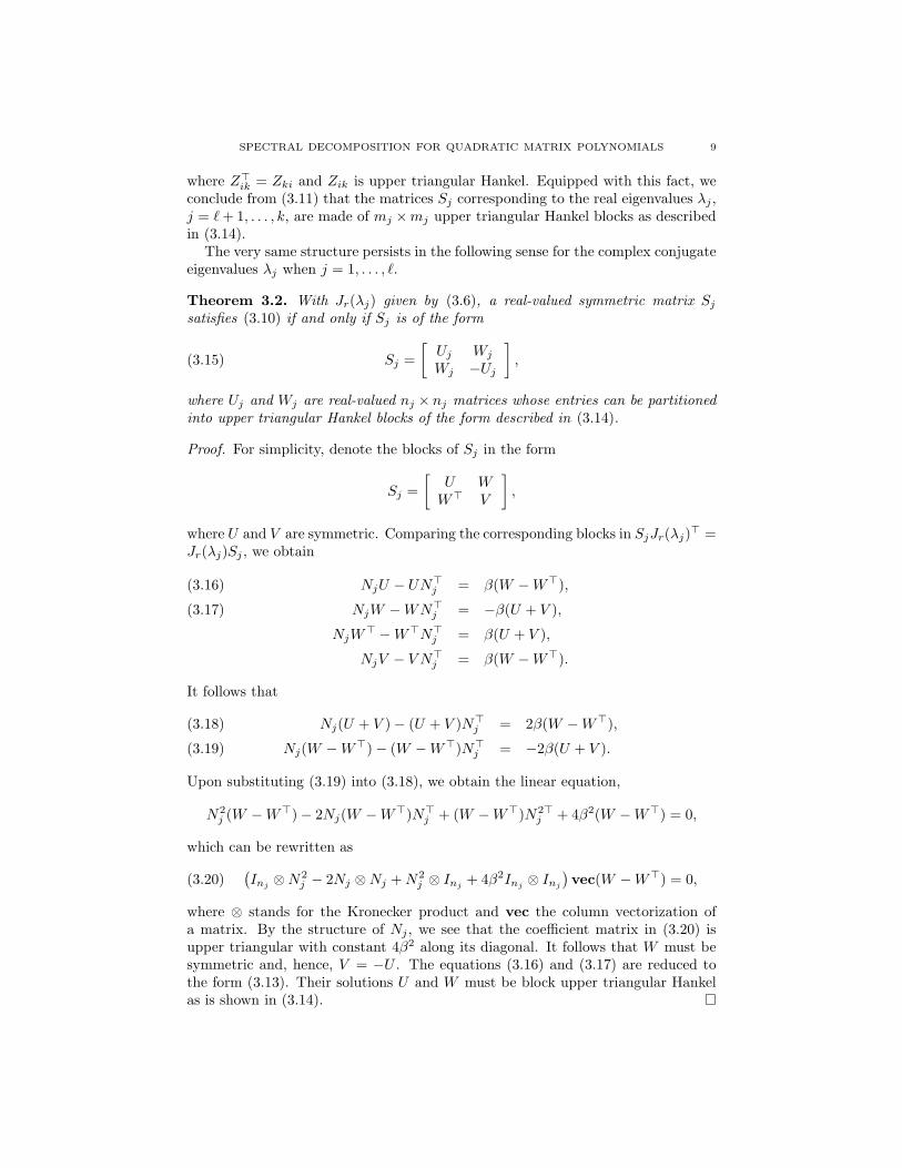
Theorem 3.2. With Jr(λj) given by (3.6), a real-valued symmetric matrix Sj

satisfies (3.10) if and only if Sj is of the form

(3.15) Sj =[

Uj Wj

Wj −Uj

],

where Uj and Wj are real-valued nj × nj matrices whose entries can be partitionedinto upper triangular Hankel blocks of the form described in (3.14).

Proof. For simplicity, denote the blocks of Sj in the form

Sj =[

U WW V

],

where U and V are symmetric. Comparing the corresponding blocks in SjJr(λj) =Jr(λj)Sj , we obtain

NjU − UNj = β(W − W),(3.16)

NjW − WNj = −β(U + V ),(3.17)

NjW − WN

j = β(U + V ),

NjV − V Nj = β(W − W).

It follows that

Nj(U + V ) − (U + V )Nj = 2β(W − W),(3.18)

Nj(W − W) − (W − W)Nj = −2β(U + V ).(3.19)

Upon substituting (3.19) into (3.18), we obtain the linear equation,

N2j (W − W) − 2Nj(W − W)N

j + (W − W)N2j + 4β2(W − W) = 0,

which can be rewritten as

(3.20)(Inj

⊗ N2j − 2Nj ⊗ Nj + N2

j ⊗ Inj+ 4β2Inj

⊗ Inj

)vec(W − W) = 0,

where ⊗ stands for the Kronecker product and vec the column vectorization ofa matrix. By the structure of Nj , we see that the coefficient matrix in (3.20) isupper triangular with constant 4β2 along its diagonal. It follows that W must besymmetric and, hence, V = −U . The equations (3.16) and (3.17) are reduced tothe form (3.13). Their solutions U and W must be block upper triangular Hankelas is shown in (3.14).

10 MOODY T. CHU AND SHU-FANG XU

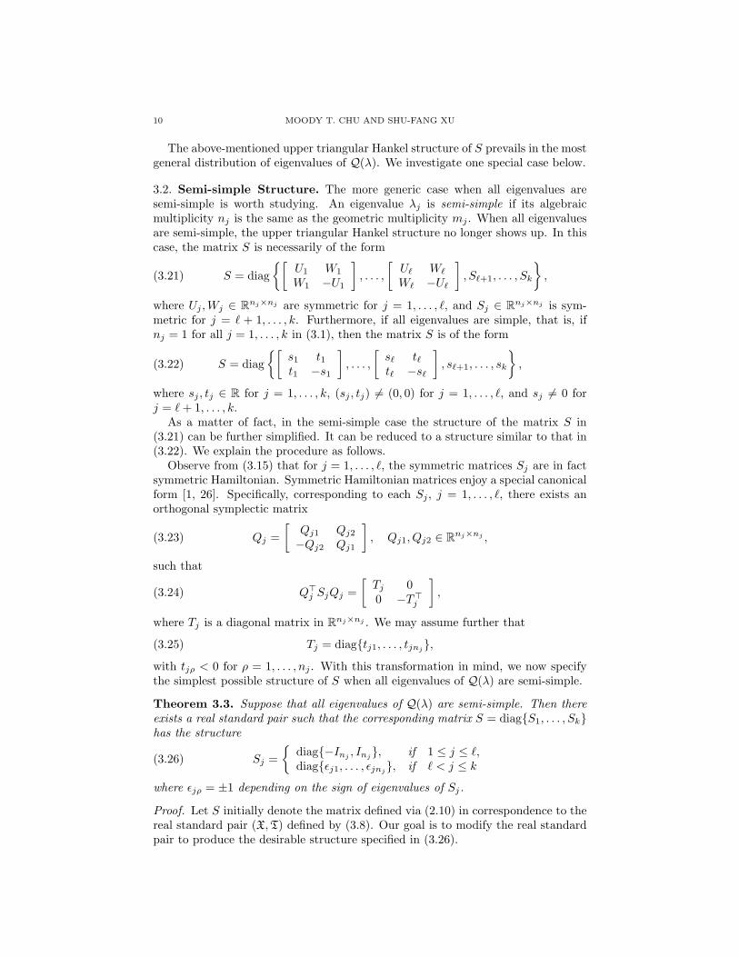
The above-mentioned upper triangular Hankel structure of S prevails in the mostgeneral distribution of eigenvalues of Q(λ). We investigate one special case below.

3.2. Semi-simple Structure. The more generic case when all eigenvalues aresemi-simple is worth studying. An eigenvalue λj is semi-simple if its algebraicmultiplicity nj is the same as the geometric multiplicity mj . When all eigenvaluesare semi-simple, the upper triangular Hankel structure no longer shows up. In thiscase, the matrix S is necessarily of the form

(3.21) S = diag[

U1 W1

W1 −U1

], . . . ,

[U W

W −U

], S+1, . . . , Sk

,

where Uj , Wj ∈ Rnj×nj are symmetric for j = 1, . . . , , and Sj ∈ Rnj×nj is sym-metric for j = + 1, . . . , k. Furthermore, if all eigenvalues are simple, that is, ifnj = 1 for all j = 1, . . . , k in (3.1), then the matrix S is of the form

(3.22) S = diag[

s1 t1t1 −s1

], . . . ,

[s tt −s

], s+1, . . . , sk

,

where sj , tj ∈ R for j = 1, . . . , k, (sj , tj) = (0, 0) for j = 1, . . . , , and sj = 0 forj = + 1, . . . , k.

As a matter of fact, in the semi-simple case the structure of the matrix S in(3.21) can be further simplified. It can be reduced to a structure similar to that in(3.22). We explain the procedure as follows.

Observe from (3.15) that for j = 1, . . . , , the symmetric matrices Sj are in factsymmetric Hamiltonian. Symmetric Hamiltonian matrices enjoy a special canonicalform [1, 26]. Specifically, corresponding to each Sj , j = 1, . . . , , there exists anorthogonal symplectic matrix

(3.23) Qj =[

Qj1 Qj2

−Qj2 Qj1

], Qj1, Qj2 ∈ R

nj×nj ,

such that

(3.24) Qj SjQj =

[Tj 00 −T

j

],

where Tj is a diagonal matrix in Rnj×nj . We may assume further that

(3.25) Tj = diagtj1, . . . , tjnj,

with tjρ < 0 for ρ = 1, . . . , nj . With this transformation in mind, we now specifythe simplest possible structure of S when all eigenvalues of Q(λ) are semi-simple.

Theorem 3.3. Suppose that all eigenvalues of Q(λ) are semi-simple. Then thereexists a real standard pair such that the corresponding matrix S = diagS1, . . . , Skhas the structure

(3.26) Sj =

diag−Inj, Inj

, if 1 ≤ j ≤ ,diagεj1, . . . , εjnj

, if < j ≤ k

where εjρ = ±1 depending on the sign of eigenvalues of Sj.

Proof. Let S initially denote the matrix defined via (2.10) in correspondence to thereal standard pair (X, T) defined by (3.8). Our goal is to modify the real standardpair to produce the desirable structure specified in (3.26).

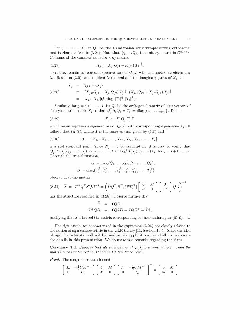
SPECTRAL DECOMPOSITION FOR QUADRATIC MATRIX POLYNOMIALS 11

For j = 1, . . . , , let Qj be the Hamiltonian structure-preserving orthogonalmatrix characterized in (3.24). Note that Qj1 + ıQj2 is a unitary matrix in Cnj×nj .Columns of the complex-valued n × nj matrix

(3.27) Xj := Xj(Qj1 + ıQj2)|Tj |12 ,

therefore, remain to represent eigenvectors of Q(λ) with corresponding eigenvalueλj . Based on (3.5), we can identify the real and the imaginary parts of Xj as

Xj = XjR + ıXjI

≡ [(XjRQj1 − XjIQj2)|Tj |12 , (XjRQj2 + XjIQj1)|Tj |

12 ](3.28)

= [XjR, XjI ]Qjdiag|Tj |12 , |Tj |

12 .

Similarly, for j = + 1, . . . , k, let Qj be the orthogonal matrix of eigenvectors ofthe symmetric matrix Sj so that Q

j SjQj = Tj := diagtj1, . . . , tjnj. Define

(3.29) Xj := XjQj |Tj |12 ,

which again represents eigenvectors of Q(λ) with corresponding eigenvalue λj . Itfollows that (X, T), where T is the same as that given by (3.8) and

(3.30) X := [X1R, X1I , . . . , XR, XI , X+1, . . . , Xk],

is a real standard pair. Since Nj = 0 by assumption, it is easy to verify thatQ

j Jr(λj)Qj = Jr(λj) for j = 1, . . . , and Qj J(λj)Qj = J(λj) for j = +1, . . . , k.

Through the transformation,

Q := diagQ1, . . . , Q, Q+1, . . . , Qk,

D := diagT121 , T

121 , . . . , T

12

, T12

, T12

+1, . . . , T12

k ,

observe that the matrix

(3.31) S := D−1QSQD−1 =(

DQ[X, (XT)][

C MM 0

] [X

XT

]QD

)−1

has the structure specified in (3.26). Observe further that

X = XQD,

XTQD = XQTD = XQDT = XT,

justifying that S is indeed the matrix corresponding to the standard pair (X, T).

The sign attributes characterized in the expression (3.26) are closely related tothe notion of sign characteristic in the GLR theory [11, Section 10.5]. Since the ideaof sign characteristic will not be used in our applications, we shall not elaboratethe details in this presentation. We do make two remarks regarding the signs.

Corollary 3.4. Suppose that all eigenvalues of Q(λ) are semi-simple. Then thematrix S characterized in Theorem 3.3 has trace zero.

Proof. The congruence transformation[In −1

2CM−1

0 In

] [C MM 0

] [In −1

2CM−1

0 In

]=

[0 MM 0

]

12 MOODY T. CHU AND SHU-FANG XU

asserts that the matrix [ C MM 0 ] has equal numbers of positive and negative eigenval-

ues. By Sylvester’s law of inertia, it follows that the parameter matrix S definedin (3.31) has equal numbers of positive and negative 1’s along its diagonal.

Finally, in contrast to (1.4) for eigenvectors of a symmetric linear pencil withpositive definite leading matrix coefficient, we conclude this section with a mostgeneral orthogonality property for eigenvectors of a real symmetric quadratic λ-matrix Q(λ).

Corollary 3.5. Suppose that all eigenvalues of Q(λ) are semi-simple. Then thereexists a real standard pair,

X = [x1R,x1I , . . . ,xR,xI ,x2+1, . . . ,x2n],

T = diag[

α1 β1

−β1 α1

], . . . ,

[α β

−β α

], λ2+1, . . . , λ2n

,

where xjR± ıxjI are complex conjugate eigenvectors associated with complex conju-gate eigenvalues αj±ıβj, j = 1, . . . , , and xj is a real-valued eigenvector associatedwith real-valued eigenvalue λj, j = 2+1, . . . , 2n; not all eigenvalues are necessarilydistinct, such that[

X

XT

] [C MM 0

] [X

XT

]= Γ := diag

[1 00 −1

], . . . ,

[1 00 −1

],(3.32) [

X

XT

] [−K 00 M

] [X

XT

]= ΓT.(3.33)

Proof. The expression (3.32) follows from rearranging the eigenvalues properly, ifnecessary, and applying Theorem 3.3 and Corollary 3.4. The expression (3.33)follows from the relationship (2.9).

The result of Corollary 3.5 can be interpreted as the simultaneous reduction ofthe pair of real symmetric matrices, [ C M

M 0 ] and[−K 0

0 M

]by real congruence. It

is important to note that for any real symmetric quadratic λ-matrix Q(λ), the“canonical” matrix Γ necessarily has equal numbers of 1’s and −1’s along its diag-onal. This is in sharp contrast to (1.4) where eigenvectors are B-orthogonal.

4. Applications

Spectral decomposition of a linear transformation is so important that it hasbecome a classic in the literature. What we have done above is to develop a theoryof spectral decomposition for real symmetric quadratic λ-matrices. In particular,we realize in Theorem 2.3 that there is a matrix S arising in the decomposition. Thematrix S plays a role of a normalization factor and, in general cases, its structureis well understood. Such knowledge can sometimes shed considerable insight intodifficult problems. In this section, we describe a few applications of this theory.Some of the problems below have been discussed elsewhere in lengthy papers, butour approach significantly simplifies the arguments.

SPECTRAL DECOMPOSITION FOR QUADRATIC MATRIX POLYNOMIALS 13

4.1. Inverse Eigenvalue Problem. Generally speaking, an inverse eigenvalueproblem is to reconstruct the coefficient matrices of a quadratic pencil from someknown information of its eigenvalues and eigenvectors. Some general discussion forlinear problems can be found in the book [6]. The quadratic inverse eigenvalueproblems are much harder. There is already a long list of studies on this subject.See, for example, [2, 16, 17, 19, 20, 21, 22, 25, 27] and the references containedtherein. In this demonstration, we consider the special QIEP where the entireeigeninformation is given:

(QIEP)] Given 2n eigenpairs (λj ,xj)2nj=1 with

λ2j−1 = λ2j = αj + ıβj , αj ∈ R, βj > 0,x2j−1 = x2j = xjR + ıxjI , xjR,xjI ∈ Rn, j = 1, 2, . . . , ,

andλj ∈ R, xj ∈ R

n, j = 2 + 1, . . . , 2n,

construct a real symmetric quadratic λ-matrix Q(λ) in the form of(1.1) so that the equations

(4.1) λ2jMxj + λjCxj + Kxj = 0,

are satisfied for all j = 1, 2, . . . , 2n. That is, Q(λ) has the prescribedset (λj ,xj)2n

j=1 as its eigenpairs.The system of equations in (4.1) can be written as

(4.2) MXΛ2 + CXΛ + KX = 0,

where

(4.3)X := [x1R,x1I , . . . ,xR,xI ,x2+1, . . . ,x2n],

Λ := diag[

α1 β1

−β1 α1

], . . . ,

[α β

−β α

], λ2+1, . . . , λ2n

.

We can immediately solve this inverse problem for almost all prescribed eigeninfor-mation by Theorems 2.3 and 2.4. Specifically, using (3.22), we have the followingresult.

Theorem 4.1. Assume that the matrix Λ has only simple eigenvalues. Then theQIEP has a solution if there is a nonsingular symmetric matrix S of the form

S = diag[

s1 t1t1 −s1

], . . . ,

[s tt −s

], s2+1, . . . , s2n

,

such that XSX = 0 and the product XΛSX is nonsingular. In this case, thematrix coefficients M , C and K of the solution Q(λ) are given by

M = (XΛSX)−1, C = −MXΛ2SXM, K = −MXΛ3SXM + CM−1C.

Now we can be more specific by taking into account some additional physicalproperties. In all cases, we find it remarkable that Theorem 4.1 provides sufficientand necessary conditions for the general solution.

Example 1. For a damped vibrating system, we may assume that all the giveneigenvalues in the QIEP are nonreal, that is, = n. In this case, it might be“tempting” to try a matrix S that is of simpler form, say,

S = diag[

1 00 −1

], . . . ,

[1 00 −1

].

14 MOODY T. CHU AND SHU-FANG XU

The condition that XSX = 0 on eigenvectors then becomes the equation

(4.4) XRXR = XIX

I ,

whereas the condition that XΛSX be nonsingular becomes that the matrix

(4.5) [XR, XI ][

−Ω UU Ω

] [XR, XI

]be nonsingular with the notation

XR := [x1R, . . . ,xnR],XI := [x1I , . . . ,xnI ],

and

Ω := diagα1, . . . , αn,U := diagβ1, . . . , βn.

We want to stress that the very brief argument above gives rise to precisely thesufficient conditions discussed in [22] for the solvability of the QIEP. Furthermore,the matrix coefficients M , C and K of the particular solution Q(λ) to the QIEPcan be expressed as

M−1 = −[XR, XI ][−Ω UU Ω

] [XR, XI

],

C = M [XR, XI ][U2 − Ω2 2UΩ

2UΩ Ω2 − U2

] [XR, XI

]M,

K = M [XR, XI ][3ΩU2 − Ω3 3UΩ2 − U3

3UΩ2 − U3 Ω3 − 3ΩU2

] [XR, XI

]M + CM−1C.

Example 2. Our quadratic λ-matrix Q(λ) is said to be hyperbolic if M ispositive definite and

(xCx)2 > 4(xMx)(xKx)for all nonzero x ∈ Rn. A hyperbolic system is said to be over-damped if, addi-tionally, C is positive definite and K is positive semi-definite. For an over-dampedsystem, it is well known that all the eigenvalues are real, nonpositive, and semi-simple [11, Theorem 13.1]. This is the case that all given eigenvalues in our QIEPare real, that is, = 0. This inverse problem has been discussed in [20]. In thiscase, we use the matrix

S = diagI,−I,and the condition XSX = 0 becomes

(4.6) X1X1 = X2X

2 ,

and the condition XΛSX being nonsingular becomes the matrix

X1Λ1X1 − X2Λ2X

2

being nonsingular with the notation

X1 := [x1, . . . ,xn],X2 := [xn+1, . . . ,x2n],

and

Λ1 = diagλ1, . . . , λn,Λ2 = diagλn+1, . . . , λ2n.

SPECTRAL DECOMPOSITION FOR QUADRATIC MATRIX POLYNOMIALS 15

Under these conditions, the corresponding matrix coefficients are then given by

M−1 = X1Λ1X1 − X2Λ2X

2 ,

C = M(X2Λ22X

2 − X1Λ2

1X1 )M,

K = M(X2Λ32X

2 − X1Λ3

1X1 )M + CM−1C.

It has to be noted, however, that the construction thus far still cannot warranta solution to the over-damped QIEP. We need to impose additional conditions onthe prescribed spectral data to ensure that these matrix coefficients are positivedefinite and that the resulting Q(λ) is over-damped. One strategy exploited in [20]is based on the facts, by (4.6), that X2 = X1Θ for some real orthogonal matrix Θand that Λ1 consists of the n largest prescribed (negative) eigenvalues. A sufficientcondition on Θ can then be characterized to guarantee that the reconstructed Q(λ)is over-damped [20, Corollary 6].

4.2. Total Decoupling Problem. It has been long desirable, yet with very lim-ited success, to characterize the dynamical behavior of a complicated high-degree-of-freedom system in terms of the dynamics of some simpler low-degree-of-freedomsubsystems. For linear pencils, there are usually modal coordinates under whichthe undamped quadratic eigenvalue problem can be represented by diagonal coeffi-cient matrices. This amounts to the simultaneous diagonalization of two matricesby congruence or equivalence transformations [15, Section 4.5]. In other words, theundamped quadratic eigenvalue problem can be totally decoupled. Most vibratingsystems, however, are quadratic and damped. It is known that three general coeffi-cient matrices M , C, and K cannot be diagonalized simultaneously by equivalenceor congruence coordinate transformations. In the literature, engineers and practi-tioners have to turn to the so-called proportionally or classically damped systemsfor the purpose of simultaneous diagonalization.

Recently, Garvey, Friswell and Prells [7] proposed a notion that total decouplingof a system is not equivalent to simultaneous diagonalization. In particular, theyargued that, under some mild assumptions, a general quadratic λ-matrix can be con-verted by real-valued isospectral transformations into a totally decoupled system.That is, a complicated n-degree-of-freedom second-order system can be reduced ton totally independent single-degree-of-freedom second-order subsystems.

Given a real symmetric quadratic λ-matrix Q(λ) in the form of (1.1), the prin-ciple idea is to seek a nonsingular matrix U ∈ R

2n×2n such that the correspondinglinearized system L(λ) defined in (2.1) is transformed into

(4.7) U[

C MM 0

]U =

[CD MD

MD 0

], U

[−K 00 M

]U =

[−KD 0

0 MD

],

where MD, CD and KD are all diagonal matrices. Such a transformation, if itexists, is isospectral, so the original pencil (1.1) is equivalent to a totally decoupledsystem

(4.8) QD(λ) := MDλ2 + CDλ + KD,

in the sense that eigenvectors x for Q(λ) and y for QD(λ) are related by[xλx

]= U

[yλy

],

provided that MD and M are nonsingular. The focus therefore is on the existenceof U .

16 MOODY T. CHU AND SHU-FANG XU

The original proof of this important result by Garvey, Friswell and Prells [7]contains some ambiguities which were later clarified and simplified by Chu and delBuono in [4]. A rather sophisticated algorithm was proposed in [5] for computing thetransformation numerically without knowing a priori the eigeninformation. Herewe offer an even simpler proof by employing the theory established in this paper.

For demonstration, assume that all the eigenvalues of Q(λ) are simple. ByCorollary 3.5, we can find eigenvalues matrix Λ and eigenvector matrix X in theform of (4.3) such that

(4.9)

[X

XΛ

] [C MM 0

] [X

XΛ

]= S := diag

[1 00 −1

], . . . ,

[1 00 −1

],[

XXΛ

] [−K 00 M

] [X

XΛ

]= SΛ.

From any given

MD = diagm1, m2, . . . , mn, 0 = mj ∈ R,

define

CD := diagc1, c2, . . . , cn,KD := diagk1, k2, . . . , kn

by

cj :=

−2mjαj , j = 1, 2, . . . , ,

−mj(λ2j−1 + λ2j), j = + 1, . . . , n,(4.10)

and

kj :=

mj(β2

j + α2j ), j = 1, 2, . . . , ,

mjλ2j−1λ2j , j = + 1, . . . , n.(4.11)

Then it is readily seen that the quadratic pencil

QD(λ) := MDλ2 + CDλ + KD

has the same spectrum as Q(λ). Let ej denote the standard jth unit vector. Directcalculation shows that for 1 ≤ j ≤ we have[

ej 0αjej βjej

] [CD MD

MD 0

] [ej 0

αjej βjej

]=

[0 βjmj

βjmj 0

],

and for + 1 ≤ j ≤ n we have[ej

λ2j−1ej

] [CD MD

MD 0

] [ej

λ2j−1ej

]= mj(λ2j−1 − λ2j),[

ej

λ2jej

] [CD MD

MD 0

] [ej

λ2jej

]= mj(λ2j − λ2j−1).

SPECTRAL DECOMPOSITION FOR QUADRATIC MATRIX POLYNOMIALS 17

Obviously, we also have

12mjβj

[1 −11 1

] [0 βjmj

βjmj 0

] [1 −11 1

]=

[1 00 −1

].

Now select values of mj such that

(4.12)

mjβj > 0, if 1 ≤ j ≤ ,mj(λ2j−1 − λ2j) > 0, if + 1 ≤ j ≤ n,

and define vectors⎧⎨⎩ [yjR,yjI ] := 1√2βjmj

[ej ,−ej ], if 1 ≤ j ≤ ,

y2j−1 = y2j := 1√mj(λ2j−1−λ2j)

ej , if + 1 ≤ j ≤ n.

Then it follows that

(4.13)

[Y

Y Λ

] [CD MD

MD 0

] [Y

Y Λ

]= S,[

YY Λ

] [−KD 0

0 MD

] [Y

Y Λ

]= SΛ,

where

Y := [y1R,y1I , . . . ,yR,yI ,y2+1, . . . ,y2n]

is the eigenvector matrix of QD(λ). Comparing (4.9) and (4.13), we conclude thatthe required nonsingular 2n × 2n matrix U can be taken as the matrix

(4.14) U =[

XXΛ

] [Y

Y Λ

]−1

.

It is worth noting that the technique employed above is constructive. A closeexamination of the procedure reveals that the assumption of simple eigenvalues isonly for convenience. The approach can be extended to the “regular systems” char-acterized in [27, Definition 8] or high order systems. Indeed, by reordering the realeigenvalues, if necessary, we may ensure positivity of mj from (4.12). Consequently,the signs of cj and kj could also be determined in (4.10) and (4.11). This featuremight be useful to meet the requirement of physical feasibility. Some relevant workson isospectral transformations can be found in [19, 27].

4.3. Eigenvalue Embedding Problem. Model updating concerns the modifica-tion of an existing but inaccurate model with measured data. For models char-acterized by a second-order dynamical system, the measured data usually involveincomplete knowledge of natural frequencies, mode shapes, or other spectral infor-mation. In conducting the updating, it is often desirable to match only the part ofobserved data without tampering with the other part of unmeasured or unknowneigenstructure inherent in the original model. Such an updating, if possible, is saidto have no spill-over. It has been shown recently that model updating with no spill-over is entirely possible for undamped quadratic systems, whereas the spill-over fordamped systems generally is unpreventable [3]. Such a difficulty is sometimes com-promised by considering the eigenvalue embedding problem (EEP), which we stateas follows [2]:

18 MOODY T. CHU AND SHU-FANG XU

(EEP) Given a real symmetric quadratic λ-matrix Q0(λ) = M0λ2

+ C0λ + K0 and a few of its associated eigenvalues λiki=1 with

k < 2n, assume that new eigenvalues µiki=1 have been measured.

Update the quadratic system Q0(λ) to Q(λ) = Mλ2 + Cλ + K sothat only the subset λik

i=1 is replaced by µiki=1 as k eigenvalues

of Q(λ) while the remaining 2n−k eigenpairs of Q(λ), which usuallyare unknown, and all the eigenvectors are kept the same as thoseof the original Q0(λ).

An iterative scheme that reassigns one eigenvalue at a time has been suggested in[2] as a possible numerical method for solving the EEP. That algorithm suffers fromtwo shortcomings — that the calculation can break down prematurely, and thatnot all desirable eigenvalues are guaranteed to be updated. Once again, using ourtheory, we offer a novel approach for solving the EEP which completely circumventsall inbuilt troubles of the algorithm proposed in [2].

For demonstration, assume that all eigenvalues of Q0(λ) are simple. Let the2n eigenpairs of Q0(λ) be (λi,xi)2n

i=1. Denote the real-valued representations of(λi,xi)k

i=1 and(λi,xi)2ni=k+1 as

Λ1 := diag[

α1 β1

−β1 α1

], . . . ,

[α1 β1

−β1 α1

], λ21+1, . . . , λk

,

X1 := [x1R,x1I , . . . ,x1R,x1I ,x21+1, . . . ,xk]

and

Λ2 := diag[

αk+1 βk+1

−βk+1 αk+1

], . . . ,

[αk+2 βk+2

−βk+2 αk+2

], λk+22+1, . . . , λ2n

,

X2 := [x(k+1)R,x(k+1)I , . . . ,x(k+2)R,x(k+2)I ,xk+22+1, . . . ,x2n],

respectively. Denote further the two matrices,

S−11 :=

[X1

X1Λ1

] [C0 M0

M0 0

] [X1

X1Λ1

],

S−12 :=

[X2

X2Λ2

] [C0 M0

M0 0

] [X2

X2Λ2

].

Then, by Theorem 2.3, we know that

M−10 = X1Λ1S1X

1 + X2Λ2S2X

2 ,

C0 = −M0

(X1Λ2

1S1X1 + X2Λ2

2S2X2

)M0,(4.15)

K0 = −M0

(X1Λ3

1S1X1 + X2Λ3

2S2X2

)M0 + C0M

−10 C0.

Denote the real-valued representation of µiki=1 by W . Assume that W has

exactly the same block diagonal structure as that of Λ1, that is, assume that W isof the form

W = diag[

γ1 δ1

−δ1 γ1

], . . . ,

[γ1 δ1

−δ1 γ1

], µ21+1, . . . , µk

.

Since the eigenvectors are not modified, the condition X1S1X1 + X2S2X

2 = 0

automatically holds. Suppose that the matrix

(4.16) X1WS1X1 + X2Λ2S2X

2

SPECTRAL DECOMPOSITION FOR QUADRATIC MATRIX POLYNOMIALS 19

is nonsingular. Then by Theorem 2.4, we know right away that one particularsolution to EEP is given by

M−1 = X1WS1X1 + X2Λ2S2X

2 ,

C = −M(X1W

2S1X1 + X2Λ2

2S2X2

)M,(4.17)

K = −M(X1W

3S1X1 + X2Λ3

2S2X2

)M + CM−1C.

Combining (4.15) with (4.17), we see that the update takes place in the followingway:

M−1 = M−10 + X1(W − Λ1)S1X

1 ,

C = M[M−1

0 C0M−10 − X1(W 2 − Λ2

1)S1X1

]M,(4.18)

K = M[M−1

0 (K0 − C0M−10 C0)M−1

0 − X1(W 3 − Λ31)S1X

1

]M + CM−1C,

provided that M−10 + X1(W − Λ1)S1X

1 is nonsingular. It is critically important

to note that the update formula (4.18) from Q0(λ) to Q(λ) does not need theinformation about (Λ2, X2).

We believe that this closed form solution for the EEP is of interest itself and isinnovative in the literature.

5. Conclusion

The classical GLR theory is a powerful methodology that generalizes the notionof spectral decomposition for linear operators to matrix polynomials of arbitrarydegrees. This paper modifies the GLR theory for the special application to realsymmetric quadratic matrix polynomials subject to the specific restriction that allmatrices in the representation be real-valued. By constructing a real standard pairin the same way described in (3.8) which includes the most general case of arbitraryalgebraic or geometric multiplicities, we characterize a special type of real-valuedspectral decomposition for real symmetric quadratic λ-matrices in terms of theusual eigeninformation.

In order to accommodate the requirement of a real-valued decomposition, aspecial matrix S is introduced. Three fundamental relationships between S ∈R2n×2n and (X, T) ∈ Rn×2n × R2n×2n, i.e., the matrix XTSX is nonsingular, theequality XSX = 0 holds, and the matrix TkS is symmetric for all k, determine anecessary and sufficient condition for the spectral decomposition. The structure ofS is investigated under different assumptions of multiplicities. In the special casewhen all eigenvalues are semi-simple, S can be taken to the special form

S = diag[

1 00 −1

], . . . ,

[1 00 −1

],

which is the generalized notion of “orthogonality” among eigenvectors of a realsymmetric quadratic matrix polynomial.

The fact that we have real-valued spectral decomposition in hand makes it con-venient for application. It is demonstrated how three nontrivial inverse problems,each of which has attracted considerable research efforts in the literature, can nowbe easily solved by exploiting our theory.

20 MOODY T. CHU AND SHU-FANG XU

Acknowledgment

The authors are deeply indebted to Professor Peter Lancaster and two otheranonymous referees for their many insightful suggestions that greatly helped us tobetter understand this subject.

References

[1] A. Bunse-Gerstner, R. Byers and V. Mehrmann, A chart of numerical methods for struc-tured eigenvalue problems, SIAM J. Matrix Anal. Appl., 13(1992), 419-453. MR1152761(93b:65063)

[2] J. Carvalho, B. N. Datta, W. W. Lin, and C. S. Wang, Symmetric preserving eigenvalueembedding in finite element model updating of vibrating structures, J. Sound Vibration,290(2006), 839–864. MR2196623 (2007d:74087)

[3] M. T. Chu, B. Datta, W. W. Lin and S. F. Xu, The spill-over phenomenon in quadraticmodel updating, AIAA J., 46(2008), 420–428.

[4] M. T. Chu and N. Del Buono, Total decoupling of a general quadratic pencil, Pt. I: Theory,J. Sound Vibration, 309(2008), 96-111.

[5] M. T. Chu and N. Del Buono, Total decoupling of a general quadratic pencil, Pt. II: Structurepreserving isospectral flows, J. Sound Vibration, 309(2008), 112–128.

[6] M. T. Chu and G. H. Golub, Inverse Eigenvalue Problems; Theory, Algorithms, and Appli-cations, Oxford University Press, Oxford, 2005. MR2263317 (2007i:65001)

[7] S. D. Garvey, M. I. Friswell, and U. Prells, Coordinate transformations for general sec-ond order systems, Pt. I: General transformations, J. Sound Vibration, 258(2002), 885–909.MR1944645 (2003k:70020)

[8] S. D. Garvey, M. I. Friswell, and U. Prells, Coordinate transformations for general secondorder systems, Pt. II: Elementary structure preserving transformations, J. Sound Vibration,258(2002), 911–930. MR1944646 (2003k:70021)

[9] F. R. Gantmacher, The Theory of Matrices, Vol. 1, Translated from the Russian by K. A.Hirsch, AMS Chelsea Publishing, Providence, RI, 1998. MR1657129 (99f:15001)

[10] I. Gohberg, P. Lancaster, and L. Rodman, Spectral analysis of selfadjoint matrix polynomials,Ann. of Math., 112(1980), 34–71. MR584074 (82c:15010)

[11] I. Gohberg, P. Lancaster, and L. Rodman, Matrix Polynomials, Computer Science and Ap-plied Mathematics. Academic Press, Inc., New York, London, 1982. MR662418 (84c:15012)

[12] I. Gohberg, P. Lancaster, and L. Rodman, Matrices and Indefinite Scalar Products,Birkhauser, Basel, 1983. MR859708 (87j:15001)

[13] P. R. Halmos, What does the spectral theorem say? Amer. Math. Monthly, 70(1963), 241-247.MR0150600 (27:595)

[14] N. J. Higham, D. S. Mackey, N. Mackey and F. Tisseur, Symmetric linearlization for matrixpolynomials, SIAM J. Matrix Anal. Appl., 29(2006), 143-159. MR2288018

[15] R. A. Horn and C. R. Johnson, Matrix Analysis, Cambridge University Press, New York,1991. MR1084815 (91i:15001)

[16] Y. C. Kuo, W. W. Lin, and S. F. Xu, Solutions of the partially described inverse quadratic

eigenvalue problem, SIAM J. Matrix Anal. Appl., 29(2006), 33-53. MR2288012 (2008a:93022)[17] P. Lancaster, Expressions for damping matrices in linear vibration problems, J. Aero-Space

Sci., 28(1961), pp. 256.[18] P. Lancaster, Lambda-matrices and Vibrating Systems, Dover Publications; Dover edition,

1966. MR0210345 (35:1238)[19] P. Lancaster, Isospectral vibrating systems. Pt. I: The spectral method, Linear Algebra Appl.,

409(2005), 51–69. MR2169546 (2006e:74043)[20] P. Lancaster, Inverse spectral problems for semi-simple damped vibrating systems, SIAM J.

Matrix Anal. Appl., 29(2007), 279–301. MR2288026[21] P. Lancaster and J. Maroulas, Inverse problems for damped vibrating systems, J. Math. Anal.

Appl., 123(1987), 238–261. MR881543 (88d:34013)[22] P. Lancaster and U. Prells, Inverse problems for damped vibrating systems, J. Sound Vibra-

tion, 283(2005), 891–914. MR2136391 (2006a:70050)[23] P. Lancaster and L. Rodman, Canonical forms for Hermitian matrix pairs under strict equiv-

alence and congruence, SIAM Review, 47(2005), 407-443. MR2178635 (2007i:15021)

SPECTRAL DECOMPOSITION FOR QUADRATIC MATRIX POLYNOMIALS 21

[24] P. Lancaster and L. Rodman, Canonical forms for symmetric/skew-symmetric real ma-trix pairs under strict equivalence and congruence, Linear Algebra Appl., 406(2005), 1-76.MR2156428 (2006d:15027)

[25] P. Lancaster and Q. Ye, Inverse spectral problems for linear and quadratic matrix pencils,Linear Algebra Appl., 107(1988), 293–309. MR960152 (89i:15016)

[26] C. Paige and C. Van Loan, A Schur decomposition for Hamiltonian matrices, Linear AlgebraAppl., 41(1981), 11-32. MR649714 (84d:65019)

[27] U. Prells and P. Lancaster, Isospectral vibrating systems. Pt. II: Structure preserving trans-formations, in Operator Theory and Indefinite Inner Product Spaces, Oper. Theory Adv.Appl., 163(2006), 275–298. MR2215867 (2006m:70043)

[28] F. Tisseur and K. Meerbergen, The quadratic eigenvalue problem, SIAM Rev., 43(2001),253–286. MR1861082 (2002i:65042)

Department of Mathematics, North Carolina State University, Raleigh, North Car-

olina 27695-8205

E-mail address: chu@math.ncsu.edu

LMAM, School of Mathematical Sciences, Peking University, Beijing, 100871, China

E-mail address: xsf@pku.edu.cn