SPATIAL RESONANCE OVERLAP IN BOSE–EINSTEIN ... - People · PDF fileho = /(m ω ho)...

International Journal of Bifurcation and Chaos, Vol. 16, No. 4 (2006) 945–959c© World Scientific Publishing Company

SPATIAL RESONANCE OVERLAP INBOSE–EINSTEIN CONDENSATES IN

SUPERLATTICE POTENTIALS

VIVIEN P. CHUAInstitute for Computational Mathematics and Engineering,

Stanford University, Stanford, CA 94305, [email protected]

MASON A. PORTERDepartment of Physics and Center for the Physics of Information,

California Institute of Technology, Pasadena, CA 91125, [email protected]

Received December 17, 2004; Revised May 31, 2005

We employ Chirikov’s overlap criterion to investigate interactions between subharmonic res-onances of coherent structure solutions of the Gross–Pitaveskii (GP) equation governing themean-field dynamics of cigar-shaped Bose–Einstein condensates in optical superlattices. Weapply a standing wave ansatz to the GP equation to obtain a parametrically forced Duffing equa-tion describing the BEC’s spatial dynamics. We then investigate analytically the dependenceof spatial resonances on the depth of the superlattice potential, deriving an order-of-magnitudeestimate for the critical depth at which spatial resonances with respect to different lattice har-monics first overlap. We also derive a formula for the size of resonance zones and examine changesin our estimates as the relative superlattice amplitudes corresponding to the different harmonicsare adjusted. We investigate the onset of global chaos and support our analytical work withnumerical simulations.

Keywords : Bose–Einstein condensates; Hamiltonian systems; Chirikov’s overlap criterion.

1. Introduction

Bose–Einstein condensation was predicted in the1920s by Satyendra Nath Bose and Albert Einsteinand was first observed experimentally in 1995 usingdilute vapors of sodium and rubidium that hadbeen cooled to temperatures near absolute zero[Anderson et al., 1995; Davis et al., 1995]. Amagnetically-trapped gas was brought to temper-atures of a few hundred nanokelvins by lasercooling, left to expand by switching off theconfining trap, and subsequently imaged with opti-cal methods. The gas was observed to reside inthe lowest quantum (ground) state, creating aBose–Einstein condensate (BEC), which consists

of several thousand to several million atoms. Asharp peak in the velocity distribution observedbelow a critical temperature indicated that con-densation had occurred [Pethick & Smith, 2002;Dalfovo et al., 1999; Ketterle, 1999; Burnett et al.,1999].

BECs are inhomogeneous, so they can beobserved in both momentum and coordinate space[Dalfovo et al., 1999]. They have two character-istic length scales: the harmonic oscillator lengthaho =

√�/(mωho) (which is on the order of a few

microns), where � is Planck’s constant, m is themass of the atomic species, and ωho = (ωxωyωz)1/3

is the geometric mean of the trapping frequencies;and the mean healing length χ = 1/

√8π|a|n,

945

946 V. P. Chua & M. A. Porter

where n is the mean density and a, the (two-body) s-wave scattering length, is determined bythe atomic species of the condensate [Pethick &Smith, 2002; Dalfovo et al., 1999; Kohler, 2002;Baizakov et al., 2002]. When a is positive, thecondensate atoms repel each other; when a is nega-tive, the atoms attract each other; and when a = 0,the atoms are in the ideal gas regime. Additionally,the scattering length can be adjusted using a mag-netic field in the vicinity of a Feshbach resonance[Donley et al., 2001].

When considering two-body, mean-fieldinteractions, the condensate wave function(“order parameter”) ψ(x, t) is described by theGross–Pitaevskii (GP) equation. When placed ina cigar-shaped trap, BECs are modeled in thequasi-one-dimensional (quasi-1D) regime, whichis valid when the transverse dimensions of thecondensate are on the order of its healing lengthand its longitudinal dimension is much largerthan its transverse ones [Bronski et al., 2001a;Bronski et al., 2001b; Bronski et al., 2001c;Dalfovo et al., 1999]. In the quasi-1D regime,one employs the 1D limit of a 3D mean-fieldtheory rather than a true 1D mean-field the-ory, which would be appropriate for transversedimensions on the order of the atomic interactionlength or the atomic size [Bronski et al., 2001a;Bronski et al., 2001b; Bronski et al., 2001c;Salasnich et al., 2002; Band et al., 2003]. In thissituation, the GP equation has one spatial dimen-sion and is written

i�ψt = −[

�2

2m

]ψxx + g|ψ|2ψ + V (x)ψ, (1)

where |ψ|2 is the number density, V (x) is an exter-nal potential, g = [4π�

2a/m][1 + O(ζ2)], and ζ =√|ψ|2|a|3 is the dilute gas parameter [Dalfovo et al.,1999; Kohler, 2002; Baizakov et al., 2002].

Potentials V (x) of interest include harmonictraps, periodic lattices, superlattices [Peil et al.,2003; Rey et al., 2004] and periodically (andquasiperiodically) perturbed harmonic traps. Theability to conduct experiments on quasi-1D BECsmotivates the study of low-dimensional modelssuch as (1). The case of periodic and quasiperi-odic potentials without a confining trap along thedimension of the lattice or superlattice is of par-ticular interest. Such potentials have been used,for example, to study Josephson effects [Anderson& Kasevich, 1998], squeezed states [Orzel et al.,

2001], Landau–Zener tunneling and Bloch oscilla-tions [Morsch et al., 2001], the transition betweensuperfluidity and Mott insulation at both the clas-sical [Smerzi et al., 2002; Cataliotti et al., 2003]and quantum [Greiner et al., 2002] levels, and con-trollable soliton manipulation [Porter et al., 2006].Moreover, with each lattice site occupied by onealkali atom in its ground state, BECs in opti-cal lattices show promise as registers in quantumcomputers [Porto et al., 2003; Vollbrecht et al.,2004].

In experiments, a weak harmonic trap is typi-cally used on top of the optical lattice or superlat-tice to prevent the particles from escaping. (Thelattice is generally turned on after the trap.) Inthis paper, we consider superlattice potentials ofthe form

V (x) = ε[V1 cos(κ1x) + V2 cos(κ2x)], (2)

where κ1 < κ2 without loss of generality, V1 =V0 cos θ, and V2 = V0 sin θ. The superlattice’sprimary wave number is κ1 and its secondarywave number is κ2. Varying θ allows one toadjust the relative contributions of the superlat-tice potential’s associated primary and secondaryharmonics. The wave numbers κi and superlatticeamplitudes Vi are also experimentally adjustable[Peil et al., 2003].

The dynamics of BECs in superlattices hasrecently started to garner some attention [Porter& Kevrekidis, 2005; van Noort et al., 2004; Louiset al., 2004; Louis et al., 2005; Eksioglu et al., 2004],as this system has novel, stable spatially extendedstates and can be used for controllable solitonmanipulation. Only the case κ2 = 3κ1, has been pre-pared experimentally [Peil et al., 2003], but super-lattices with other ratios (such as 2κ2 = 3κ1) canbe constructed by adjusting the laser beams used tocreate the optical superlattice. In the present work,we consider all real ratios κ2/κ1. The superlatticepotential (2) is quasiperiodic when κ2/κ1 is irra-tional and periodic when it is rational.

The remainder of this paper is organized as fol-lows. In Sec. 2, we derive a parametrically forcedDuffing oscillator, which describes the condensate’sspatial dynamics, by applying a coherent structureansatz to the GP equation (1). This is followed by adiscussion in Sec. 3 of Chirikov’s overlap criterion,which we apply to attractive BECs with both pos-itive and negative chemical potentials to estimatethe lattice height required for the onset of glob-ally chaotic dynamics. We also derive an expression

Spatial Resonance Overlap in BEC in Superlattice Potentials 947

for the size of resonance zones. In Sec. 4, we com-pare our analytical estimates to numerically com-puted Poincare sections. We summarize our resultsin Sec. 5.

2. Coherent Structures

We consider uniformly propagating coherent struc-tures with the ansatz

ψ(x, t) = R(x) exp(i [θ(x) − µt]), (3)

where R is the amplitude of the wave function,θ(x) determines its phase, v ∝ ∇θ is the parti-cle velocity, and µ is the BEC’s chemical potential.When the (temporally periodic) coherent structure(3) is also spatially periodic, it is called a modu-lated amplitude wave (MAW) [Brusch et al., 2000;Brusch et al., 2001]. The orbital stability of MAWsfor the cubic NLS with elliptic function poten-tials has been studied by Bronski and co-authors[Bronski et al., 2001a; Bronski et al., 2001b;Bronski et al., 2001c]. To obtain stability informa-tion with sinusoidal potentials, one takes the limitas the elliptic modulus k approaches zero [Lawden,1989; Rand, 1994].

Substituting (3) into the GP equation (1) andequating real and imaginary parts yields

�µR(x) = − �2

2mR′′(x) +

[�

2

2m[θ′(x)]2

+ gR2(x) + V (x)]R(x), (4)

0 =�

2

2m[2θ′(x)R′(x) + θ′′(x)R(x)

].

This, in turn, yields the following nonautonomous,two-dimensional system of nonlinear ordinary dif-ferential equations [Bronski et al., 2001b; Porter &Cvitanovic, 2004a, 2004b]:

R′ = PR,

P ′R =

c2

R3− 2mµR

�+

2mg

�2R3 +

2m�2

V (x)R,(5)

where ′ denotes differentiation with respect to x andthe parameter c, determined by θ′(x) = c/R2, playsthe role of “angular momentum” [Bronski et al.,2001b].

When c = 0, Eq. (3) describes a standing wave.In this situation, Eq. (5) becomes

R′′ + δR + αR3 + εRV1 cos(κ1x)+ εRV2 cos(κ2x) = 0, (6)

where δ = 2mµ/�, α = −2mg/�2, and ε = −(2m/�

2)V0. We assume that the lattice depth is shallow,so that |ε| � 1.

The unperturbed Hamiltonian (correspondingto (6) with ε = 0) is

H(R,PR) =12P 2

R +12δR2 +

14αR4. (7)

KAM theory guarantees that locally chaoticdynamics occurs near resonances for arbitrarilysmall ε > 0 [Guckenheimer & Holmes, 1983;Lichtenberg & Lieberman, 1992]. Perturbations ofHamiltonian systems that break integrability leadto increasingly large regions of chaotic dynamicsin phase space as the size of the perturbation isincreased. Locally chaotic configurations have smallregions of phase space with trajectories that behaveerratically, but such trajectories still remain withinthose regions. Under sufficiently large nonintegrableforcing, however, trajectories travel from one regionof phase space to another, leading to global chaos[Lichtenberg & Lieberman, 1992; Rand, 1994].

In this work, we employ Chirikov’s overlap cri-terion to estimate the value of ε at which thedynamics of (6) first becomes globally chaotic[Rand, 1994; Lichtenberg & Lieberman, 1992].Chaotic regions in phase space are identified fromfuzziness in Poincare sections, whereas integrabletrajectories are represented by continuous curves.In the context of BECs, increasing ε correspondsto increasing the depth of the wells in the opticalsuperlattice. Fixing the other physical parameters,we examine the development of chaotic dynam-ics through spatial resonance overlap as the lat-tice depth (which can be tuned experimentally) isincreased.

It is also important to keep experimentallimitations in mind. We do not incorporate a weakharmonic trap in (6), assuming instead that thesuperlattice is present for all x. From an experi-mental perspective, it cannot be ignored after somefinite number of lattice minima. Thus far, BECsin regular optical lattices with up to 200 wells havebeen created experimentally [Pedri et al., 2001]. Theuse of infinitely many wells is a standard theoreticalapproximation and the resonance overlap we studypertains experimentally to a finite number of wells


away from the edges of the weak trap, for which it ispermissible to ignore perturbations due to the trap.

3. Chirikov’s Overlap Criterion

Chirikov’s overlap criterion is used to studythe transition from local to global chaos inHamiltonian systems. The last remaining KAMsurface between primary resonances is destroyedwhen the sum of the half-widths of the two islandseparatrices formed by the resonances equals thedistance between the resonances. The system’sHamiltonian is used to estimate the minimal per-turbation strength ε for which these separatricesbegin to touch. We derive analytical approxima-tions for the locations and sizes of the resonancezones to estimate this critical ε when the twoprimary resonances first overlap, leading to theonset of global chaos [Rand, 1994; Lichtenberg &Lieberman, 1992].

A Hamiltonian system has the form

dqi

dx=

∂H

∂pi,

dpi

dx= −∂H

∂qi, i ∈ {1, . . . , n}, (8)

where the Hamiltonian H = H(qi, pi, x; ε) can beexpanded in a power series in ε as follows:

H(qi, pi, x; ε) = H0(qi, pi, x) + εH1(qi, pi, x)+ ε2H2(qi, pi, x) + O(ε3). (9)

The nonintegrable Hamiltonian of the paramet-rically forced Duffing equation (which is a nonlinearMathieu equation) (6) is

H =12P 2

R +12δR2 +

14αR4 + ε

R2

2V1 cos(κ1x)

+ εR2

2V2 cos(κ2x). (10)

We set ε = 0 to consider the unforced (integrable)system,

R′′ + δR + αR3 = 0, (11)

which we solve approximately by keeping a singleharmonic,

R = A cos(ωx),

PR = R′ = −Aω sin(ωx).(12)

One can alternatively solve (11) exactly using ellip-tic functions, as has been done previously for appli-cations of Chirikov’s overlap criterion to nonlinearMathieu equations [Zounes & Rand, 2001, 2002a,2002b]. We substitute (12) into (11) and neglect allharmonics beyond {cos(ωx), sin(ωx)} to obtain an

approximate expression for ω as a function of A,

ω =s

δ +34αA2 . (13)

The next step is to transform to approximateaction-angle variables. Suppose the angle is givenby q = ωx, so that

R = A cos q, q′ = ω =s

δ +34αA2. (14)

The action variable p is then defined so that

q′ =∂H0

∂p=

∂H0

∂A

∂A

∂p=

sδ +

34αA2, (15)

where ∂H0/∂A = δA + (9/8)αA3. This yields thedifferential equation,

∂p

∂A=

δA +98αA3

sδ +

34αA2

, (16)

governing the dependence of p on A.We substitute (12) into (10) and neglect higher

harmonics to obtain

H =12δA2 +

932

αA4

+ εA2

2cos2 q[V1 cos(κ1x) + V2 cos(κ2x)]. (17)

We consider attractive (a < 0) condensates withboth positive (µ > 0) and negative (µ < 0) chemi-cal potentials, although only the derivation for thelatter case is presented explicitly in this paper. Thesame method works for attractive BECs with pos-itive chemical potentials [Zounes & Rand, 2001,2002a].

For negative chemical potentials, the parame-ters are rescaled so that α = 1 and δ = −1, whichwe substitute into (16) and (17) to obtain

∂p

∂A=

−A +98A3

s−1 +

34A2

(18)

and

H = −12A2 +

932

A4

+ εA2

2cos2 q[V1 cos(κ1x) + V2 cos(κ2x)] . (19)

We integrate (18) to yield

p =14A2

√−4 + 3A2 , (20)


which implies that

A =13

√2d1/3 + 8d−1/3 + 4 , (21)

where d = 8 + 243p2 + 9p√

48 + 729p2.This gives an approximate canonical transfor-

mation from (R,PR) → (q, p):

R =13

√2d1/3 + 8d−1/3 + 4 cos q,

PR = −ω

3

√2d1/3 + 8d−1/3 + 4 sin q.

(22)

The Hamiltonian (10) is thus written

H =172

[d1/3 + 4d−1/3 + 2]2

− 19[d1/3 + 4d−1/3 + 2]

+ε

9[d1/3 + 4d−1/3 + 2]

× cos2 q[V1 cos(κ1x) + V2 cos(κ2x)]. (23)

3.1. Near-identity transformations

In this section, we apply a near-identity transforma-tion to the nonautonomous Hamiltonian (23). Thistransformation has the general form [Rand, 1994;Guckenheimer & Holmes, 1983]

qi = Qi + εΘ(1)i (Qj , Pj) + ε2Θ(2)

i (Qj, Pj) + O(ε3),

pi = Pi + εΦ(1)i (Qj, Pj) + ε2Φ(2)

i (Qj , Pj) + O(ε3),(24)

where Θ(k)i and Φ(k)

i are chosen so that the trans-formation is canonical.

First, we extend phase space, so that (23) iswritten

H = H + p2

=172

[d1/31 + 4d−1/3

1 + 2]2

− 19[d1/3

1 + 4d−1/31 + 2]

+ε

9[d1/3

1 + 4d−1/31 + 2]

× cos2 q1[V1 cos(κ1q2) + V2 cos(κ2q2)] + p2

≡ H0 + εH1, (25)

where d1 = 8 + 243p21 + 9p1

√48 + 729p2

1, p1 = p,q1 = q, and q2 = x. (The variable p2 is the conju-gate momentum of q2.) The O(1) and O(ε) terms

in the transformed Hamiltonian are then

H0(qi, pi) =172

[d1/31 + 4d−1/3

1 + 2]2

− 19[d1/3

1 + 4d−1/31 + 2] + p2,

H1(qi, pi) =19[d1/3

1 + 4d−1/31 + 2]

× cos2 q1[V1 cos(κ1q2) + V2 cos(κ2q2)].

We use trigonometric identities to isolate harmonicsand obtain

H1(qi, pi) =136

[d1/31 + 4d−1/3

1 + 2]

×{V1[cos(2q1 + κ1q2)+ cos(2q1 − κ1q2) + 2 cos(κ1q2)]+ V2[cos(2q1 + κ2q2) + cos(2q1

−κ2q2) + 2 cos(κ2q2)]}. (26)

We define another near-identity transforma-tion, from (qi, pi) → (Qi, Pi) as

qi = Qi + ε∂W1

∂Pi+ O(ε2),

pi = Pi − ε∂W1

∂Qi+ O(ε2).

(27)

We choose a generating function W1 to simplify thetransformed Hamiltonian, K = K0 + εK1 + O(ε2),given by

K0 = H0(Qi, Pi)

=172

[D1/31 + 4D−1/3

1 + 2]2

− 19[D1/3

1 + 4D−1/31 + 2] + P2,

K1 = H1(Qi, Pi) + {H0,W1}

=136

[D1/31 + 4D−1/3

1 + 2]

×{V1[cos(2Q1 + κ1Q2) + cos(2Q1 − κ1Q2)+ 2 cos(κ1Q2)] + V2[cos(2Q1 + κ2Q2)+ cos(2Q1 − κ2Q2) + 2 cos(κ2Q2)]}

−h∂W1

∂Q1− ∂W1

∂Q2, (28)

where D1 = 8 + 243P 21 + 9P1

√48 + 729P 2

1, h =(M/108)[D1/3

1 +4D−1/31 +2][D−2/3

1 −4D−4/31 ]−(M/27)

[D−2/31 + 4D−4/3

1 ], M = 486P1 + 9√

48 + 729P 21 +

6561P 21/

√48 + 729P 2

1, and {H0,W1} is the Poissonbracket of H0 and W1 [Rand, 1994; Goldstein, 1980].


The appropriate generating function has theform

W1 = C1+ sin(2Q1 + κ1Q2) + C1

− sin(2Q1 − κ1Q2)

+ C2+ sin(2Q1 + κ2Q2) + C2

− sin(2Q1 − κ2Q2)+ 2C3 sin(κ1Q2) + 2C4 sin(κ2Q2). (29)

We choose W1 so that the Poisson bracket {H0,W1}eliminates all the trigonometric terms in K1 exceptfor a single term, a so-called “nonremovable” termpertaining to the resonance zone of interest. Thereare four possible choices for this term, which havecorresponding prefactors Ci

+ and Ci− for i ∈ {1, 2}.One chooses i = 1 to examine resonances withrespect to the primary lattice harmonic and i = 2for resonances with respect to the secondaryharmonic.

The coefficients C1+, C1−, C2

+, C2−, C3, and C4

are given by the formulas

Ci+ =

[D1/31 + 4D−1/3

1 + 2]Vi

36(2h + κi),

Ci− =[D1/3

1 + 4D−1/31 + 2]Vi

36(2h − κi), i ∈ {1, 2},

C3 =[D1/3

1 + 4D−1/31 + 2]V1

36,

C4 =[D1/3

1 + 4D−1/31 + 2]V2

36.

(30)

The denominators in Ci+ and Ci− vanish, respec-

tively, when 2h+κi = 0 and 2h−κi = 0, indicatingthe presence of resonance zones. In the calculationbelow, we consider resonances with respect to lat-tice harmonics due to the latter condition. We findthe locations and sizes of these resonance zonesand use Chirikov’s overlap criterion to estimatethe value of ε at which globally chaotic dynamicsoccurs.

We obtain [Rand, 1994]

K(i)1 =

Vi

36[D1/3

1 + 4D−1/31 + 2]

× [cos(2Q1 − κiQ2)], i ∈ {1, 2}, (31)

which yields the transformed Hamiltonian

K(i) =172

[D1/31 + 4D−1/3

1 + 2]2

− 19[D1/3

1 + 4D−1/31 + 2] + P2

+ εVi

36[D1/3

1 + 4D−1/31 + 2]

× [cos(2Q1 − κiQ2)] + O(ε2). (32)

3.2. Analytical estimate of thecritical lattice height

We obtain an autonomous, one degree-of-freedomsystem (for a given i ∈ {1, 2}) with a linear, canon-ical transformation,

X1 = 2Q1 − κiQ2, X2 = Q2

Y1 = P1, Y2 = P2 + κiP1.

The resulting Hamiltonian is

K(i) =172

[G1/31 + 4G−1/3

1 + 2]2

− 19[G1/3

1 + 4G−1/31 + 2] + Y2 − κiY1

+ εVi

36[G1/3

1 + 4G−1/31 + 2] cos X1 + O(ε2),

(33)

where G1 = 8 + 243Y 21 + 9Y1

√48 + 729Y 2

1 .After the transformation, X2 is no longer

explicitly present in K(i) so both Y2 and K(i) areconstant of motions [Rand, 1994]. Therefore,

K∗(i) = K(i) − Y2

=172

[G1/31 + 4G−1/3

1 + 2]2

− 19[G1/3

1 + 4G−1/31 + 2] − κiY1

+ εVi

36[G1/3

1 + 4G−1/31 + 2] cos(X1) + O(ε2)

= constant. (34)

We determine the equilibria from Hamilton’sequations,

Y ′1 = −∂K∗(i)

∂X1= ε

Vi

36[G1/3

1 + 4G−1/31 + 2] sin X1,

X ′1 =

∂K∗(i)

∂Y1

=N

108(G1/3

1 + 4G−1/31 + 2)(G−2/3

1 − 4G−4/31 )

− N

27(G−2/3

1 − 4G−4/31 )

−κi + εViN

108(G−2/3

1 − 4G−1/31 ) cos(X1),

(35)

where N = 486Y1 + 9(96Y1 + 2916Y 31)/(2Y1√

48 + 729Y 21).


The condition Y ′1 = 0 implies that equilibria

(X∗1 , Y ∗

1 ) satisfy sin X∗1 = 0, so that X∗

1 = 0 orX∗

1 = π. Substituting these values into (35) forX ′

1 = 0 gives Y ∗1 . For small ε, both values of X∗

1

give

Y ∗(i) ≈ −0.843 + 2.161κi + O(ε), (36)

where we have employed a power series expansionto approximate the value of Y ∗(i). The integrableHamiltonian (34) has a pendulum-like separatrix.We denote the location of its saddles by Y

(i)s and

its maximum height by Y(i)m . One obtains Y

(i)s when

X1 = π, and Y(i)m occurs at the same angle (X1 = 0)

as the center point of (35) and has the same Hamil-tonian value as the saddles (because it too lies onthe separatrix). Therefore,

K∗(X∗1 = 0, Y1 = Y (i)

m )

= K∗(X∗1 = π, Y1 = Y (i)

s ), i ∈ {1, 2}. (37)

This gives the equation

172

[G(i)m

1/3+ 4G(i)

m−1/3

+ 2]2

− 19[G(i)

m

1/3+ 4G(i)

m

−1/3+ 2] − κiY

(i)m

+ εVi

36[G(i)

m

1/3+ 4G(i)

m

−1/3+ 2]

=172

[G(i)1/3

s + 4G(i)−1/3

s + 2]2

− 19[G(i)1/3

s + 4G(i)−1/3

s + 2] − κiY(i)s

− εVi

36[G(i)1/3

s + 4G(i)s

−1/3+ 2], (38)

where G(i)m = 8 + 243Y (i)2

m + 9Y (i)m

r48 + 729Y (i)2

m ,

G(i)s = 8 + 243Y (i)2

s + 9Y (i)s

r48 + 729Y (i)2

s , Y(i)m =

Y(i)s + δi is to be determined, and Y

(i)s ≈ −0.843 +

2.161κi is known.We set δi = ki

√ε + O(ε) and write Eq. (38) in

the form

F (Y (i)s + ki

√ε) + εB(Y (i)

s + ki

√ε)

= F (Y (i)s ) − εB(Y (i)

s ) , (39)

where F (Y (i)s ) = (1/72)[G(i)1/3

s + 4G(i)−1/3

s + 2]2 −(1/9)(G(i)1/3

s + 4G(i)−1/3

s +2)−κiY(i)s and B(Y (i)

s ) =

(Vi/36)[G(i)1/3

s + 4G(i)−1/3

s + 2].

We expand (39) in a power series in√

ε

using F (Y (i)s + ki

√ε) = F (Y (i)

s ) +√

εF ′(Y (i)s )ki +

(1/2)εF ′′(Y (i)s )k2

i + O(ε3/2) to obtain

F (Y (i)s ) +

√εF ′(Y (i)

s )ki +12εF ′′(Y (i)

s )k2i

+εB(Y (i)s ) + O(ε3/2) = F (Y (i)

s ) − εB(Y (i)s ).(40)

At O(√

ε), we see that F ′(Y (i)s ) = 0. At O(ε), we

obtain

ki = 2

√√√√√√−B(Y (i)s )

∂2F

∂Y(i)2s

, i ∈ {1, 2}. (41)

Recall that κ2 > κ1. As ε is increased, individualresonance regions associated with each of the lat-tice harmonics begin to overlap when the minimumof the separatrix height Y

(2)m for the κ2 resonance

band equals the maximum of the separatrix heightY

(1)m of the κ1 resonance band. Equation (41) also

gives an estimate for the separatrix size, which is

Wi = 2δi = 2ki

√ε + O(ε). (42)

Resonance overlap occurs when

−0.843 + 2.161κ2 − k2

√ε

= −0.843 + 2.161κ1 + k1

√ε, (43)

which yields the order-of-magnitude estimate

εcr ≈ [2.161]2(

κ2 − κ1

k1 + k2

)2

≈ 4.670(

κ2 − κ1

k1 + k2

)2

(44)

for the critical lattice height at which the transi-tion from local to global chaos occurs. We simi-larly obtain an equation to estimate the criticalε for α = 1 and δ = 1 with the same analyticalprocedure:

−3.908 + 3.430κ2 − k2

√ε

= −3.908 + 3.430κ1 + k1

√ε. (45)

While our analysis is only guaranteed togive an order-of-magnitude estimate for εcr, ournumerical simulations (discussed in the next sec-tion) reveal that this estimate can sometimesperform far better in practice. By construction,estimates obtained using Chirikov’s overlap cri-terion give an upper bound for εcr because oneis examining the overlap of resonance bandswhen all pertinent KAM tori have been destroyed[Lichtenberg & Lieberman, 1992; Rand, 1994].Strictly speaking, the series approximation (36)


removes this guarantee, but one still nearly alwaysobtains upper bounds in practice. (In particular,our estimate provided an upper bound for everyexample we studied.)

4. Numerical Simulations

To support our analytical work, we numerically sim-ulated Eq. (6) for several values of V1 = V0 cos(θ)and V2 = V0 sin(θ). We examined situations withdifferent relative contributions of the two latticeharmonics. Specifically, we considered θ = nπ/16for n ∈ {1, . . . , 7}. (When θ = 0 and θ = π/2, oneof the forcing terms is identically zero, so only oneresonance is being excited.) In our simulations, wescaled (6) so that V0 = 1.

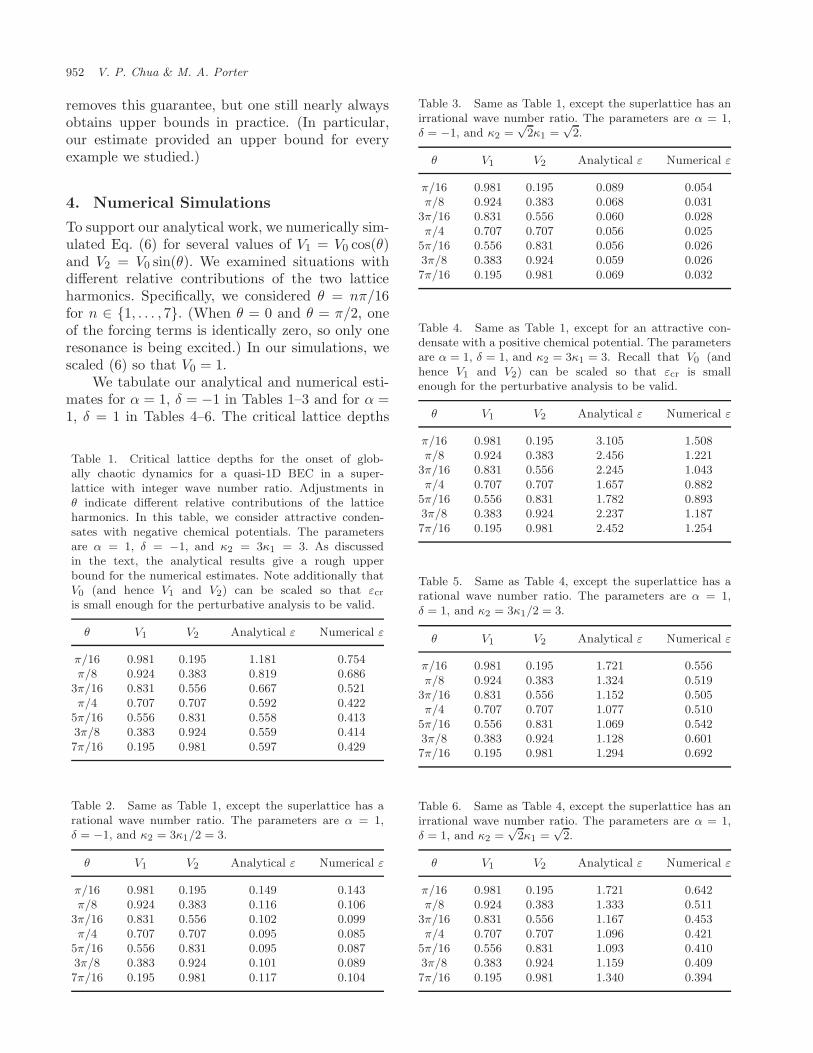
We tabulate our analytical and numerical esti-mates for α = 1, δ = −1 in Tables 1–3 and for α =1, δ = 1 in Tables 4–6. The critical lattice depths

Table 1. Critical lattice depths for the onset of glob-ally chaotic dynamics for a quasi-1D BEC in a super-lattice with integer wave number ratio. Adjustments inθ indicate different relative contributions of the latticeharmonics. In this table, we consider attractive conden-sates with negative chemical potentials. The parametersare α = 1, δ = −1, and κ2 = 3κ1 = 3. As discussedin the text, the analytical results give a rough upperbound for the numerical estimates. Note additionally thatV0 (and hence V1 and V2) can be scaled so that εcr

is small enough for the perturbative analysis to be valid.

θ V1 V2 Analytical ε Numerical ε

π/16 0.981 0.195 1.181 0.754π/8 0.924 0.383 0.819 0.686

3π/16 0.831 0.556 0.667 0.521π/4 0.707 0.707 0.592 0.422

5π/16 0.556 0.831 0.558 0.4133π/8 0.383 0.924 0.559 0.4147π/16 0.195 0.981 0.597 0.429

Table 2. Same as Table 1, except the superlattice has arational wave number ratio. The parameters are α = 1,δ = −1, and κ2 = 3κ1/2 = 3.


π/16 0.981 0.195 0.149 0.143π/8 0.924 0.383 0.116 0.106

3π/16 0.831 0.556 0.102 0.099π/4 0.707 0.707 0.095 0.085

5π/16 0.556 0.831 0.095 0.0873π/8 0.383 0.924 0.101 0.0897π/16 0.195 0.981 0.117 0.104

Table 3. Same as Table 1, except the superlattice has anirrational wave number ratio. The parameters are α = 1,δ = −1, and κ2 =

√2κ1 =

√2.


π/16 0.981 0.195 0.089 0.054π/8 0.924 0.383 0.068 0.031

3π/16 0.831 0.556 0.060 0.028π/4 0.707 0.707 0.056 0.025

5π/16 0.556 0.831 0.056 0.0263π/8 0.383 0.924 0.059 0.0267π/16 0.195 0.981 0.069 0.032

Table 4. Same as Table 1, except for an attractive con-densate with a positive chemical potential. The parametersare α = 1, δ = 1, and κ2 = 3κ1 = 3. Recall that V0 (andhence V1 and V2) can be scaled so that εcr is smallenough for the perturbative analysis to be valid.


π/16 0.981 0.195 3.105 1.508π/8 0.924 0.383 2.456 1.221

3π/16 0.831 0.556 2.245 1.043π/4 0.707 0.707 1.657 0.882

5π/16 0.556 0.831 1.782 0.8933π/8 0.383 0.924 2.237 1.1877π/16 0.195 0.981 2.452 1.254

Table 5. Same as Table 4, except the superlattice has arational wave number ratio. The parameters are α = 1,δ = 1, and κ2 = 3κ1/2 = 3.


π/16 0.981 0.195 1.721 0.556π/8 0.924 0.383 1.324 0.519

3π/16 0.831 0.556 1.152 0.505π/4 0.707 0.707 1.077 0.510

5π/16 0.556 0.831 1.069 0.5423π/8 0.383 0.924 1.128 0.6017π/16 0.195 0.981 1.294 0.692

Table 6. Same as Table 4, except the superlattice has anirrational wave number ratio. The parameters are α = 1,δ = 1, and κ2 =

√2κ1 =

√2.


π/16 0.981 0.195 1.721 0.642π/8 0.924 0.383 1.333 0.511

3π/16 0.831 0.556 1.167 0.453π/4 0.707 0.707 1.096 0.421

5π/16 0.556 0.831 1.093 0.4103π/8 0.383 0.924 1.159 0.4097π/16 0.195 0.981 1.340 0.394


for κ2/κ1 = 3 are shown in Tables 1 and 4, thosefor κ2/κ1 = 3/2 are shown in Tables 2 and 5, andthose for κ2/κ1 =

√2 are shown in Tables 3 and

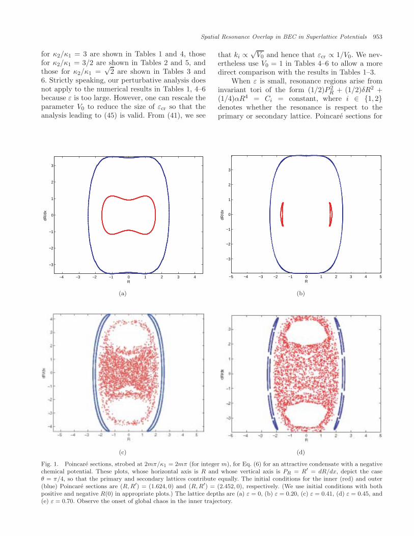
6. Strictly speaking, our perturbative analysis doesnot apply to the numerical results in Tables 1, 4–6because ε is too large. However, one can rescale theparameter V0 to reduce the size of εcr so that theanalysis leading to (45) is valid. From (41), we see

that ki ∝√

V0 and hence that εcr ∝ 1/V0. We nev-ertheless use V0 = 1 in Tables 4–6 to allow a moredirect comparison with the results in Tables 1–3.

When ε is small, resonance regions arise frominvariant tori of the form (1/2)P 2

R + (1/2)δR2 +(1/4)αR4 = Ci = constant, where i ∈ {1, 2}denotes whether the resonance is respect to theprimary or secondary lattice. Poincare sections for

−4 −3 −2 −1 0 1 2 3 4

−3

−2

−1

0

1

2

3

R

dR/d

x

(a)

−5 −4 −3 −2 −1 0 1 2 3 4 5

−3

−2

−1

0

1

2

3

R

dR/d

x

(b)

(c) (d)

Fig. 1. Poincare sections, strobed at 2mπ/κ1 = 2mπ (for integer m), for Eq. (6) for an attractive condensate with a negativechemical potential. These plots, whose horizontal axis is R and whose vertical axis is PR = R′ = dR/dx, depict the caseθ = π/4, so that the primary and secondary lattices contribute equally. The initial conditions for the inner (red) and outer(blue) Poincare sections are (R, R′) = (1.624, 0) and (R, R′) = (2.452, 0), respectively. (We use initial conditions with bothpositive and negative R(0) in appropriate plots.) The lattice depths are (a) ε = 0, (b) ε = 0.20, (c) ε = 0.41, (d) ε = 0.45, and(e) ε = 0.70. Observe the onset of global chaos in the inner trajectory.


(e)

Fig. 1. (Continued )

an attractive BEC with a negative chemical poten-tial and parameters κ1 = 1, κ2 = 3κ1 = 3,θ = π/4, and ε = 0, 0.20, 0.41, 0.45, 0.70,are depicted in Fig. 1. (Numerical integration wasperformed using a Runge–Kutta integrator withstep size 0.01.) The inner curves correspond to res-onances with respect to the primary lattice har-monic. The outer curves correspond to resonanceswith respect to the secondary lattice harmonic.

Initial conditions for the inner and outer curveswere obtained by substituting Y ∗(i) = P

(i)1 ≈ p

(i)1 =

p(i) and q(i) = 0 for i ∈ {1, 2} into (22) to deter-mine R(0) when R′(0) = 0. (The approximationof P

(i)1 by p

(i)1 is better for smaller ε and exact for

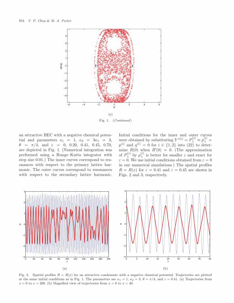
ε = 0. We use initial conditions obtained from ε = 0in our numerical simulations.) The spatial profilesR = R(x) for ε = 0.41 and ε = 0.45 are shown inFigs. 2 and 3, respectively.

0 20 40 60 80 100 120 140 160 180 200−3

−2

−1

0

1

2

3

x

R

(a)

0 5 10 15 20 25 30 35 40−3

−2

−1

0

1

2

3

x

R

(b)

Fig. 2. Spatial profiles R = R(x) for an attractive condensate with a negative chemical potential. Trajectories are plottedat the same initial conditions as in Fig. 1. The parameters are κ1 = 1, κ2 = 3, θ = π/4, and ε = 0.41. (a) Trajectories fromx = 0 to x = 200. (b) Magnified view of trajectories from x = 0 to x = 40.


(a)

0 5 10 15 20 25 30 35 40−3

−2

−1

0

1

2

3

x

R

(b)

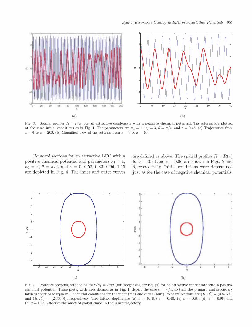
Fig. 3. Spatial profiles R = R(x) for an attractive condensate with a negative chemical potential. Trajectories are plottedat the same initial conditions as in Fig. 1. The parameters are κ1 = 1, κ2 = 3, θ = π/4, and ε = 0.45. (a) Trajectories fromx = 0 to x = 200. (b) Magnified view of trajectories from x = 0 to x = 40.

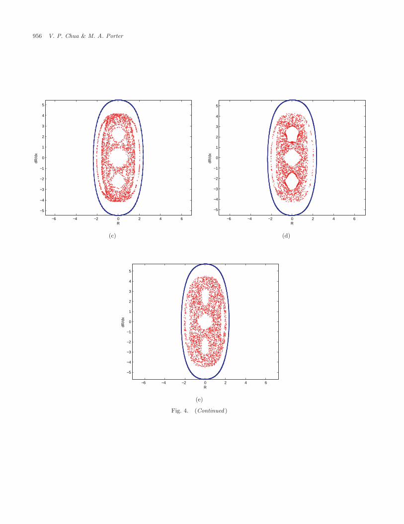
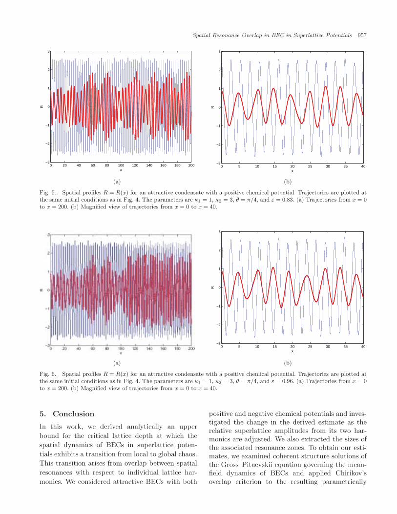
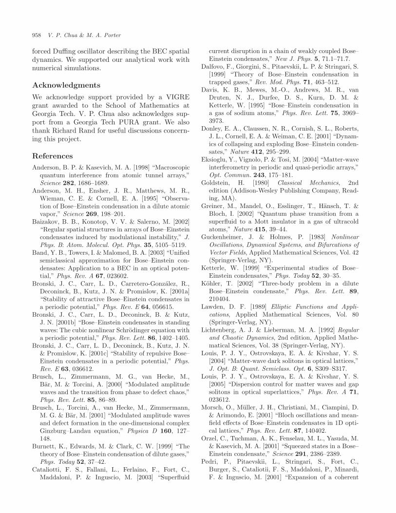
Poincare sections for an attractive BEC with apositive chemical potential and parameters κ1 = 1,κ2 = 3, θ = π/4, and ε = 0, 0.52, 0.83, 0.96, 1.15are depicted in Fig. 4. The inner and outer curves

are defined as above. The spatial profiles R = R(x)for ε = 0.83 and ε = 0.96 are shown in Figs. 5 and6, respectively. Initial conditions were determinedjust as for the case of negative chemical potentials.

−5 −4 −3 −2 −1 0 1 2 3 4 5

−4

−3

−2

−1

0

1

2

3

4

R

dR/d

x

(a) (b)

Fig. 4. Poincare sections, strobed at 2mπ/κ1 = 2mπ (for integer m), for Eq. (6) for an attractive condensate with a positivechemical potential. These plots, with axes defined as in Fig. 1, depict the case θ = π/4, so that the primary and secondarylattices contribute equally. The initial conditions for the inner (red) and outer (blue) Poincare sections are (R,R′) = (0.873, 0)and (R,R′) = (2.366, 0), respectively. The lattice depths are (a) ε = 0, (b) ε = 0.40, (c) ε = 0.83, (d) ε = 0.96, and(e) ε = 1.15. Observe the onset of global chaos in the inner trajectory.


−6 −4 −2 0 2 4 6

−5

−4

−3

−2

−1

0

1

2

3

4

5

R

dR/d

x

(c)

−6 −4 −2 0 2 4 6

−5

−4

−3

−2

−1

0

1

2

3

4

5

R

dR/d

x

(d)

−6 −4 −2 0 2 4 6

−5

−4

−3

−2

−1

0

1

2

3

4

5

R

dR/d

x

(e)

Fig. 4. (Continued )


0 20 40 60 80 100 120 140 160 180 200−3

−2

−1

0

1

2

3

x

R

(a)

0 5 10 15 20 25 30 35 40−3

−2

−1

0

1

2

3

x

R

(b)

Fig. 5. Spatial profiles R = R(x) for an attractive condensate with a positive chemical potential. Trajectories are plotted atthe same initial conditions as in Fig. 4. The parameters are κ1 = 1, κ2 = 3, θ = π/4, and ε = 0.83. (a) Trajectories from x = 0to x = 200. (b) Magnified view of trajectories from x = 0 to x = 40.

(a)

0 5 10 15 20 25 30 35 40−3

−2

−1

0

1

2

3

x

R

(b)

Fig. 6. Spatial profiles R = R(x) for an attractive condensate with a positive chemical potential. Trajectories are plotted atthe same initial conditions as in Fig. 4. The parameters are κ1 = 1, κ2 = 3, θ = π/4, and ε = 0.96. (a) Trajectories from x = 0to x = 200. (b) Magnified view of trajectories from x = 0 to x = 40.

5. Conclusion

In this work, we derived analytically an upperbound for the critical lattice depth at which thespatial dynamics of BECs in superlattice poten-tials exhibits a transition from local to global chaos.This transition arises from overlap between spatialresonances with respect to individual lattice har-monics. We considered attractive BECs with both

positive and negative chemical potentials and inves-tigated the change in the derived estimate as therelative superlattice amplitudes from its two har-monics are adjusted. We also extracted the sizes ofthe associated resonance zones. To obtain our esti-mates, we examined coherent structure solutions ofthe Gross–Pitaevskii equation governing the mean-field dynamics of BECs and applied Chirikov’soverlap criterion to the resulting parametrically


forced Duffing oscillator describing the BEC spatialdynamics. We supported our analytical work withnumerical simulations.

Acknowledgments

We acknowledge support provided by a VIGREgrant awarded to the School of Mathematics atGeorgia Tech. V. P. Chua also acknowledges sup-port from a Georgia Tech PURA grant. We alsothank Richard Rand for useful discussions concern-ing this project.

References

Anderson, B. P. & Kasevich, M. A. [1998] “Macroscopicquantum interference from atomic tunnel arrays,”Science 282, 1686–1689.

Anderson, M. H., Ensher, J. R., Matthews, M. R.,Wieman, C. E. & Cornell, E. A. [1995] “Observa-tion of Bose–Einstein condensation in a dilute atomicvapor,” Science 269, 198–201.

Baizakov, B. B., Konotop, V. V. & Salerno, M. [2002]“Regular spatial structures in arrays of Bose–Einsteincondensates induced by modulational instability,” J.Phys. B: Atom. Molecul. Opt. Phys. 35, 5105–5119.

Band, Y. B., Towers, I. & Malomed, B. A. [2003] “Unifiedsemiclassical approximation for Bose–Einstein con-densates: Application to a BEC in an optical poten-tial,” Phys. Rev. A 67, 023602.

Bronski, J. C., Carr, L. D., Carretero-Gonzalez, R.,Deconinck, B., Kutz, J. N. & Promislow, K. [2001a]“Stability of attractive Bose–Einstein condensates ina periodic potential,” Phys. Rev. E 64, 056615.

Bronski, J. C., Carr, L. D., Deconinck, B. & Kutz,J. N. [2001b] “Bose–Einstein condensates in standingwaves: The cubic nonlinear Schrodinger equation witha periodic potential,” Phys. Rev. Lett. 86, 1402–1405.

Bronski, J. C., Carr, L. D., Deconinck, B., Kutz, J. N.& Promislow, K. [2001c] “Stability of repulsive Bose–Einstein condensates in a periodic potential,” Phys.Rev. E 63, 036612.

Brusch, L., Zimmermann, M. G., van Hecke, M.,Bar, M. & Torcini, A. [2000] “Modulated amplitudewaves and the transition from phase to defect chaos,”Phys. Rev. Lett. 85, 86–89.

Brusch, L., Torcini, A., van Hecke, M., Zimmermann,M. G. & Bar, M. [2001] “Modulated amplitude wavesand defect formation in the one-dimensional complexGinzburg–Landau equation,” Physica D 160, 127–148.

Burnett, K., Edwards, M. & Clark, C. W. [1999] “Thetheory of Bose–Einstein condensation of dilute gases,”Phys. Today 52, 37–42.

Cataliotti, F. S., Fallani, L., Ferlaino, F., Fort, C.,Maddaloni, P. & Inguscio, M. [2003] “Superfluid

current disruption in a chain of weakly coupled Bose–Einstein condensates,” New J. Phys. 5, 71.1–71.7.

Dalfovo, F., Giorgini, S., Pitaevskii, L. P. & Stringari, S.[1999] “Theory of Bose–Einstein condensation intrapped gases,” Rev. Mod. Phys. 71, 463–512.

Davis, K. B., Mewes, M.-O., Andrews, M. R., vanDruten, N. J., Durfee, D. S., Kurn, D. M. &Ketterle, W. [1995] “Bose–Einstein condensation ina gas of sodium atoms,” Phys. Rev. Lett. 75, 3969–3973.

Donley, E. A., Claussen, N. R., Cornish, S. L., Roberts,J. L., Cornell, E. A. & Weiman, C. E. [2001] “Dynam-ics of collapsing and exploding Bose–Einstein conden-sates,” Nature 412, 295–299.

Eksioglu, Y., Vignolo, P. & Tosi, M. [2004] “Matter-waveinterferometry in periodic and quasi-periodic arrays,”Opt. Commun. 243, 175–181.

Goldstein, H. [1980] Classical Mechanics, 2ndedition (Addison-Wesley Publishing Company, Read-ing, MA).

Greiner, M., Mandel, O., Esslinger, T., Hansch, T. &Bloch, I. [2002] “Quantum phase transition from asuperfluid to a Mott insulator in a gas of ultracoldatoms,” Nature 415, 39–44.

Guckenheimer, J. & Holmes, P. [1983] NonlinearOscillations, Dynamical Systems, and Bifurcations ofVector Fields, Applied Mathematical Sciences, Vol. 42(Springer-Verlag, NY).

Ketterle, W. [1999] “Experimental studies of Bose–Einstein condensates,” Phys. Today 52, 30–35.

Kohler, T. [2002] “Three-body problem in a diluteBose–Einstein condensate,” Phys. Rev. Lett. 89,210404.

Lawden, D. F. [1989] Elliptic Functions and Appli-cations, Applied Mathematical Sciences, Vol. 80(Springer-Verlag, NY).

Lichtenberg, A. J. & Lieberman, M. A. [1992] Regularand Chaotic Dynamics, 2nd edition, Applied Mathe-matical Sciences, Vol. 38 (Springer-Verlag, NY).

Louis, P. J. Y., Ostrovskaya, E. A. & Kivshar, Y. S.[2004] “Matter-wave dark solitons in optical lattices,”J. Opt. B: Quant. Semiclass. Opt. 6, S309–S317.

Louis, P. J. Y., Ostrovskaya, E. A. & Kivshar, Y. S.[2005] “Dispersion control for matter waves and gapsolitons in optical superlattices,” Phys. Rev. A 71,023612.

Morsch, O., Muller, J. H., Christiani, M., Ciampini, D.& Arimondo, E. [2001] “Bloch oscillations and mean-field effects of Bose–Einstein condensates in 1D opti-cal lattices,” Phys. Rev. Lett. 87, 140402.

Orzel, C., Tuchman, A. K., Fenselau, M. L., Yasuda, M.& Kasevich, M. A. [2001] “Squeezed states in a Bose–Einstein condensate,” Science 291, 2386–2389.

Pedri, P., Pitaevskii, L., Stringari, S., Fort, C.,Burger, S., Cataliotii, F. S., Maddaloni, P., Minardi,F. & Inguscio, M. [2001] “Expansion of a coherent


array of Bose–Einstein condensates,” Phys. Rev. Lett.87, 220401.

Peil, S., Porto, J. V., Laburthe Tolra, B., Obrecht, J. M.,King, B. E., Subbotin, M., Rolston, S. L. & Phillips,W. D. [2003] “Patterned loading of a Bose–Einsteincondensate into an optical lattice,” Phys. Rev. A 67,051603(R).

Pethick, C. J. & Smith, H. [2002] Bose–Einstein Conden-sation in Dilute Gases (Cambridge University Press,Cambridge, UK).

Porter, M. A. & Cvitanovic, P. [2004a] “Modulatedamplitude waves in Bose–Einstein condensates,”Phys. Rev. E, 047201.

Porter, M. A. & Cvitanovic, P. [2004b] “A perturba-tive analysis of modulated amplitude waves in Bose–Einstein condensates,” Chaos 14, 739–755.

Porter, M. A. & Kevrekidis, P. G. [2005] “Bose–Einsteincondensates in superlattices,” Siam. J. App. Dyn.Syst. 4, 783–807.

Porter, M. A., Kevrekidis, P. G., Carretero Gonzalez, R.& Frantzeskakis, D. J. [2006] “Dynamics and manip-ulation of matter-wave solitons in optical superlat-tices,” Phys. Lett. A 352, 210–215.

Porto, J. V., Rolston, S., Laburthe Tolra, B., Williams,C. J. & Phillips, W. D. [2003] “Quantum informationwith neutral atoms as qubits,” Philo. Trans.: Math.Phys. Engin. Sci. 361, 1417–1427.

Rand, R. H. [1994] Topics in Nonlinear Dynamicswith Computer Algebra, Computation in Education:Mathematics, Science and Engineering, Vol. 1(Gordon and Breach Science Publishers, USA).

Rey, A. M., Hu, B., Calzetta, E., Roura, A. & Clark, C.[2004] “Nonequilibrium dynamics of optical lattice-loaded BEC atoms: Beyond HFB approximation,”Phys. Rev. A 69, 033610.

Salasnich, L., Parola, A. & Reatto, L. [2002] “Periodicquantum tunnelling and parametric resonance withcigar-shaped Bose–Einstein condensates,” J. Phys. B:Atom. Molec. Opt. Phys. 35, 3205–3216.

Smerzi, A., Trombettoni, A., Kevrekidis, P. G. &Bishop, A. R. [2002] “Dynamical superfluid-insulatortransition in a chain of weakly coupled Bose–Einsteincondensates,” Phys. Rev. Lett. 89, 170402.

van Noort, M., Porter, M. A., Yi, Y. & Chow, S.-N.[2004] “Quasiperiodic and chaotic dynamics in Bose–Einstein condensates in periodic lattices and super-lattices,” e-print: arXiv:math.DS/0405112.

Vollbrecht, K. G. H., Solano, E. & Cirac, J. L. [2004]“Ensemble quantum computation with atoms in peri-odic potentials,” Phys. Rev. Lett. 93, 220502.

Zounes, R. S. & Rand, R. H. [2001] “Global behavior ofa nonlinear quasiperiodic Mathieu equation,” in Proc.DETC2001, 2001 ASME Design Engineering Techni-cal Conf., No. VIB-21595, pp. 1–11.

Zounes, R. S. & Rand, R. H. [2002a] “Global behavior ofa nonlinear quasiperiodic Mathieu equation,” Nonlin.Dyn. 27, 87–105.

Zounes, R. S. & Rand, R. H. [2002b] “Subharmonic res-onance in the non-linear Mathieu equation,” Int. J.Non-Lin. Mech. 37, 43–73.

SPATIAL RESONANCE OVERLAP IN BOSE–EINSTEIN ... - People · PDF fileho = /(m ω ho)...

Documents

Transcript of SPATIAL RESONANCE OVERLAP IN BOSE–EINSTEIN ... - People · PDF fileho = /(m ω ho)...