Sparsity and the Possibility of Inferencebickel/BickelYan2009sankh...Sparsity and the possibility of...
24
Sankhy¯a : The Indian Journal of Statistics 2008, Volume 70, Part 1, pp. 0-23 c 2008, Indian Statistical Institute Sparsity and the Possibility of Inference Peter J. Bickel University of California, Berkeley, USA Donghui Yan University of California, Berkeley, USA Abstract We discuss the importance of sparsity in the context of nonparametric regres- sion and covariance matrix estimation. We point to low manifold dimension of the covariate vector as a possible important feature of sparsity, recall an estimate of dimension due to Levina and Bickel (2005) and establish some conjectures made in that paper. AMS (2000) subject classification. Primary 62-02, 62G08, 62G20, 62J10. Keywords and phrases. Sparsity, statistical inference, nonparametric regres- sion, covariance matrix estimation, dimension estimation. 1 Introduction In a pathbreaking RSS discussion paper in 1995, Donoho, Johnstone, Hoch and Stern pointed out the importance of sparsity. Subsequent im- portant work by Donoho, Johnstone and collaborators (1995-2006) focused mainly on sparsity in the form of sparse linear representations of regression functions and the like when estimation is carried out using overcomplete dictionaries. My own appreciation of the importance of sparsity came from the following observation that grew out of conversations with my late friend and colleague, Leo Breiman. Stone (1977) considered the estimation of regression functions η(X)= E(Y X) 1 Both authors were supported under NSF Grant DMS0605236. 2 P. Bickel is responsible for Sections 1-3. Section 4 is based on the work of D. Yan.
Transcript of Sparsity and the Possibility of Inferencebickel/BickelYan2009sankh...Sparsity and the possibility of...
Sankhya : The Indian Journal of Statistics2008, Volume 70, Part 1, pp. 0-23c! 2008, Indian Statistical Institute
Sparsity and the Possibility of Inference
Peter J. BickelUniversity of California, Berkeley, USA
Donghui YanUniversity of California, Berkeley, USA
Abstract
We discuss the importance of sparsity in the context of nonparametric regres-sion and covariance matrix estimation. We point to low manifold dimensionof the covariate vector as a possible important feature of sparsity, recall anestimate of dimension due to Levina and Bickel (2005) and establish someconjectures made in that paper.
AMS (2000) subject classification. Primary 62-02, 62G08, 62G20, 62J10.Keywords and phrases. Sparsity, statistical inference, nonparametric regres-sion, covariance matrix estimation, dimension estimation.
1 Introduction
In a pathbreaking RSS discussion paper in 1995, Donoho, Johnstone,Hoch and Stern pointed out the importance of sparsity. Subsequent im-portant work by Donoho, Johnstone and collaborators (1995-2006) focusedmainly on sparsity in the form of sparse linear representations of regressionfunctions and the like when estimation is carried out using overcompletedictionaries. My own appreciation of the importance of sparsity came fromthe following observation that grew out of conversations with my late friendand colleague, Leo Breiman.
Stone (1977) considered the estimation of regression functions
!(X) = E(Y!
!X)
1Both authors were supported under NSF Grant DMS0605236.2P. Bickel is responsible for Sections 1-3. Section 4 is based on the work of D. Yan.
Sparsity and the possibility of inference 1
on the basis of i.i.d. observations, (Xi,Yi), with X ! Rd, assuming onlythat ! has smoothness of order s, e.g., bounded partial derivatives of orders. He obtained the result that, from a minimax (least favorable) point ofview, estimation in the root mean square sense could not be achieved at arate greater than n! s
2s+d .
Qualitatively, what this said to us was that unless we assume an unwar-ranted degree of smoothness for the function we are estimating, the samplesizes required to get reasonable accuracy are larger that anything possiblyavailable. For example, if s = 2, d = 12, n = 104, n! s
2s+d "= .33.
Of course, in principle, constants may favor performance, s may be verylarge, but the qualitative conclusion is that if Nature is out to get us, wehave no chance with today’s very high dimensional data with poorly un-derstood models. Yet in practice there routinely are remarkable successes.Here is a table of high dimensional data sets with large to small n where highprediction accuracy has been achieved. R corresponds to misclassificationprobability.
Table 1. Some empirical evidence
d classes n R
ZIP code digits 256 10 10,000 <0.025Microarrays 3-4000 2-3 70-100 0.08
spam 57 2 4,600 <0.07
What are possible explanations? I believe in Einstein’s words that “Godis subtle but not malicious”.
In the next two sections we will discuss the meaning and consequencesof sparsity in two contexts, regression and covariance matrix estimation andrelate them to some extent.
Roughly speaking we will discuss sparse data, by which we mean pointslying on or near a low dimensional sub-manifold of a high dimensional spaceand sparse models, ones whose probability structures are characterized bylow dimensional parameters.
Our treatment is extremely sketchy and covers only a very small part ofa huge and growing body of literature. Key topics such as Bayesian methodsare only briefly pointed to at the end. But we hope this will only be one of thefirst of many review papers of aspects of modern statistics which we believe
2 Peter J. Bickel and Donghui Yan
are both novel and of key importance. In a final more technical section, wetake the opportunity to analyze and essentially settle some conjectures onnonparametric dimension estimation raised in Levina and Bickel (2005).
2 Sparsity Issues in Nonparametric Regression
Consider the regression model we introduced in the introduction
Y = !(X) + ! (2.1)
where E(!|X) = 0 and for simplicity we take ! " N (0,"2) independent of X.We specify the family of possible probability distributions of (X,Y) by P.
There are two familiar paradigms. One is linear regression where f1, ..., fp :X #$ R is given and
!(X) = fT (X)",f = (f1, ..., fp)T (2.2)
for " ! Rp unknown. The other is nonparametric regression where !(X)belongs to “a nice function space”, e.g., X = Rd,Ps % {|Dk#|(.) & K <', 1 & k & s}.
A theoretical goal is to obtain a minimax procedure, !(X), such that,
supP
EP(!(X) ( Y)2 = min!
supP
EP(!(X) ( Y)2 (2.3)
or EP(!(X)(Y)2 is “small” for P ! P. The standard solution to predictionfor linear regression
!(x) = fT (x)"
is least squares,
" = [F T F ]!1F T Y (2.4)
where FN"p ) ||fj(Xi)||, yielding as predictions
Y = F [F T F ]!1F TY (2.5)
#(x) = "T f(x). (2.6)
We are faced with the “Overfitting” problem,
E|Y ( F T "|2 ="2p
n(2.7)
Sparsity and the possibility of inference 3
where F T " is the best predictor of Y if " is known. Note that if p > n,then " is unidentifiable; if p
n $ ', then Y is worthless.
In the nonparametric case, p = '. The standard solution is, if X = Rd
to find a basis f1, ..., fp, ..., such that for ! ! Ps,
maxP
E(!(X) ( fTp (X)"p)
2 $ 0
where fp(x) = (f1(x), ..., fp(x))T and regularize. For a review of regulariza-tion - see Bickel and Li (2007) for instance. Some standard solutions are tochoose p so that
"($) = arg min"p,p
"
|Y ( fTp "p|2 + $|"p|r
#
r = 2 Ridge Regressionr = 1 LASSO
$
,$ $ 0.
There are many other methods - see, for example, references in Candesand Tao (2007) discussion, and Hastie, Tibshirani, and Friedman (2001).
All such methods can be interpreted as estimating “sparse” - low dimen-sional approximations to ! in the belief that these are adequate. It is in factmethods such as these which yield Stone’s rates. But they do not thereforea priori eliminate our di!culty, since we identify approximate sparsity withsmoothness of !. There are however often classes of models, we shall referto as sparse models (SM) which do - and these are, in some form, familiarfrom classical statistics. By SM we think of model families, such as
a) E(Y |X) =%d
j=1 gj(Xj) (Additive models)
Type a) are the natural generalizations of no interaction models inANOVA. They were introduced by Breiman and Friedman (1985) andas one might expect correspond to di!culty d = 1.
b) There exists S * {1, ..., d} such that |S| + min(d, n) and
(i) {Xj : j ! S} , {Xk : k ! Sc}(ii) Y , {Xk : k ! Sc}(iii) E(Y |X) = E(Y |Xj : j ! S)
Note that Xj are used generically and could be (known) functions of originalX1, ...,Xd.
4 Peter J. Bickel and Donghui Yan
Type b) corresponds to the belief that most variables Xj are irrelevantin that they are independent of both Y and the set of relevant variables inS.
The other main feature of regression models which makes Table 1 possibleis, we believe, the presence of what we call “Sparse data” (SD). By SD wemean, X lives on (or close to) M, a m dimensional Riemannian manifoldX = Td"1(U) for U ! O * Rm,m + d, T 1-1 and smooth or |X(T (U)| & !for some U . Note a special case is that M is a hyperplane, and this leads toprincipal components regression.
Of course, one can have both, irrelevant variables corresponding to SMand predictors highly correlated with each other as well as Y. It is, however,clear that the irrelevant variables have to be removed before we can takeadvantage of the correlated good predictors - since independent variablesresult in high dimension.
It is worth pointing out that the goal we are focusing on here is predictionand sparsity really means being well approximable by low dimensional linearsubmodels. This is di"erent from the goal of model selection where there isimplicitly a belief that the data has been generated by an !(x) for whichmost of the "j are 0.
For prediction, for instance, we choose $ in the lasso so as to ensure op-timal prediction for a smoothness class P with f1(.), ..., fk(.), ..., a completebasis for representing #(.) in P. Then, we expect most estimated coe!cientsof the fj(x) to be small but not necessarily 0. This choice of $ does not leadto what is known as consistency, which is defined by: If !(x) has (sparsest)representation
!(x) =&
{"jfj(x) : j ! S} ,
then the "j of the estimated ! are -= 0 i" j ! S. On the other hand, thechoice of $ which does lead to consistency does not yield the best minimaxprediction risks - see for instance Atkinson (1980) and Yang (2005) for adiscussion. However, nothing prevents us from first optimizing for predictionand then doing model selection or vice versa, see Fan and Lv (2008) forinstance. These questions are still being explored. We believe the practicalquestion is di"erent. With Box (1979) we agree that,
“All models are false but some models are useful”.
Our real interest is in determining which “factors” among X1, ...,Xd are“important”. A possibly more fruitful but yet unexplored point of view is
Sparsity and the possibility of inference 5
to isolate all models of dimension at most m whose predictive power is closeto optimal and then study the factors which appear in these.
Bickel and Li (2007) studied the theoretical e"ect on nonparametric re-gression if the high dimensional vector of covariates satisfies our notion ofSD. They noted that, if the manifold is unknown, employing local linearor higher order regression methods using the d dimensional covariates butchoosing the bandwidth by cross validation or some other data determinedway yields the same minimax risks as if X ! Rm rather than X ! Rd.But see also Niyogi (2007). This result can be thought of as the nonlinearanalogue of the observation that for prediction collinearity of predictive vari-ables is immaterial since the p in (2.7) is the dimension of the linear spaceof predictors.
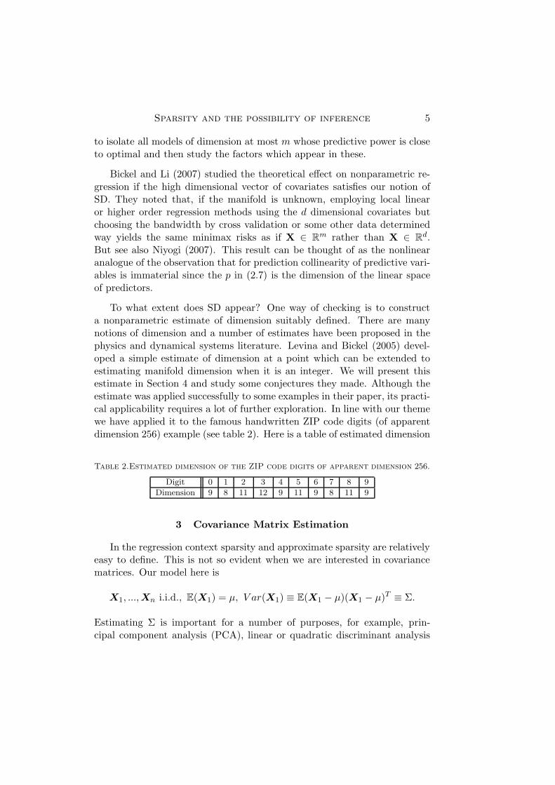
To what extent does SD appear? One way of checking is to constructa nonparametric estimate of dimension suitably defined. There are manynotions of dimension and a number of estimates have been proposed in thephysics and dynamical systems literature. Levina and Bickel (2005) devel-oped a simple estimate of dimension at a point which can be extended toestimating manifold dimension when it is an integer. We will present thisestimate in Section 4 and study some conjectures they made. Although theestimate was applied successfully to some examples in their paper, its practi-cal applicability requires a lot of further exploration. In line with our themewe have applied it to the famous handwritten ZIP code digits (of apparentdimension 256) example (see table 2). Here is a table of estimated dimension
Table 2.Estimated dimension of the ZIP code digits of apparent dimension 256.
Digit 0 1 2 3 4 5 6 7 8 9Dimension 9 8 11 12 9 11 9 8 11 9
3 Covariance Matrix Estimation
In the regression context sparsity and approximate sparsity are relativelyeasy to define. This is not so evident when we are interested in covariancematrices. Our model here is
X1, ...,Xn i.i.d., E(X1) = µ, V ar(X1) ) E(X1 ( µ)(X1 ( µ)T ) #.
Estimating # is important for a number of purposes, for example, prin-cipal component analysis (PCA), linear or quadratic discriminant analysis
6 Peter J. Bickel and Donghui Yan
(LDA/QDA), inferring independence and conditional independence (graph-ical models), implicit estimation of linear regression, #!1
XX#XY with X
regressors and Y the response.
Through recent results in random matrix theory a major pathology ofthe empirical covariance matrix has been pointed out. The eigenstructureis inconsistent for i.i.d. component models as soon as p
n $ c > 0 - seeJohnstone and Lu (2008) for a review.
We have implicitly noted in the previous section that when used in re-gression, i.e., least squares, using the empirical covariance matrix is a partof least squares which breaks down even for prediction. Bickel and Levina(2004) point out the breakdown of LDA when p
n $ '.
These problems do not simply emerge because we use the empirical co-variance matrix, as the minimax results of the previous section suggest. Theissue is again that, without sparsity assumptions, estimation of large covari-ance matrices is hopeless. A number of notions of sparsity are discussed inBickel and Levina (2008)(i)(ii). The simplest is permutation invariant spar-sity where,
A) Each row of # is sparse or sparsely approximable in operator norm,e.g., Si = {j : "ij -= 0} and |Si| & s for all i
or
B) Each row of #!1 is sparsely approximable.
Each allows estimation of the inverse but the conditions are di"erent. SeeEl Karoui (2008) for a more general notion. Note the interpretations of A),B) in the Gaussian case where,
A) Xi , Xj for all j ! Sci
or
B) Xi , Xj | Xk, k -= j, j ! Sci where Si ) {j : "ij -= 0}.
If sparsity is present as in the regression case, regularization can lead toexcellent performance. A forthcoming issue of the Annals of Statistics willcontain a number of papers including some of those cited as well as othersrelating to the area.
Sparsity and the possibility of inference 7
One salient feature of all approaches is that in the presence of sparsity,log p
n $ 0 is enough for interesting and very compelling conclusions for generalproblems. This is an area of continuing research which may shed light on thesparsity issues in regression as well. For instance, it is appealing to estimatethe inverse covariance matrix of X taking advantaging of potential sparsityand estimate the covariances of X and Y sparsely and put them togetherin a sparse version of least squares.
Even more than in regression, the order in which things are done mayalso matter. Is it good to first estimate the covariance matrix sparsely andthen look at its eigenstructure and inverses or aim at each feature of thematrix separately? Approaches of this type may be found in d’Aspremontet al (2007) and Johnstone and Lu (2008) and El Karoui (2007) .
There are two topics we have not touched on which are of key importanceand need much additional work
1. The choice, in practice, of regularization parameters for methods thattake advantage of sparsity. Theoretical order of magnitude is wellunderstood, but is of little value in this choice. We have great faithin V fold cross validation - see Bickel and Levina (2008)(ii) for oneanalysis.
2. Bayesian methods. There is clearly an intimate link between regu-larization in both regression and covariance estimation and Bayesianmethods. But in high dimensional situations which Bayesian meth-ods are trustworthy from a frequentist point of view remains to beexplored.
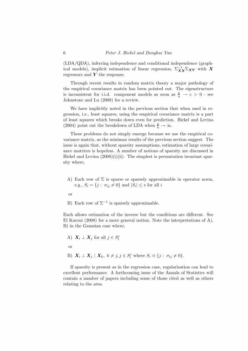
4 Some Results on Dimension Estimation
Levina and Bickel (2005) proposed the following estimator for the “true”dimension of a high dimensional dataset
mk =1
n
n&
i=1
mk(Xi)
where mk(x) is defined as
mk(x) =' 1
k ( 1
k!1&
j=1
logRk
Rj(x)
(!1! (W (x))!1
8 Peter J. Bickel and Donghui Yan
and Rj(x) is the j(th nearest neighbor distance to x ! Rm.
Here mk(x) is a local estimate of dimension and may be more usefulthan the global estimate mk. We will state and prove three theorems aboutestimation of the “true” dimension m where X1, ...,Xn are a sample of ddimensional observations, which however take their values with probability1 in a flat smooth manifold of dimension m, and have a smooth density withrespect to Lebesgue measure on Rm. What we mean by this is explainedin the statement of Theorem 4.1 on local dimension estimation below. Alltheorems can be viewed as proving corrected versions of conjectures in Levinaand Bickel (2005).
Our first theorem deals with the local estimate. The idea of the proof isto establish the result for the case X is uniformly distributed locally on themanifold and the manifold is locally described as an a!ne transformationof the m-cube. For the uniform case, we can first apply the delta methodand then employ some known distributional results. The next theorem dealswith the more di!cult global behavior which we carefully establish only forthe uniform. We only make a second moment calculation and use a theoremof Chatterjee for distributional results. The main observation is that the co-variance contribution occurs only if k-th nearest neighbor spheres intersectwhich means that the corresponding centers are no more than O((k/n)
1m )
apart. But that event occurs with probability O( kn). The rest of the ar-
gument rests upon scaling two such spheres, one centered at 0, and theirintersection by a common factor. A stronger distributional result due toYukich (2008) was brought to our attention. His proof is both more elegantand more general. Nevertheless, we believe our more special method whichyields both order bounds as k, n $ ' and local results is worth considering.
Theorem 1. Let Um"1 be a r.v. in Rm. If Um"1 " f with f twice con-tinuously di!erentiable. Xd"1 = TU !
m"1 where T = (T1, ...,Td)! . T(u) !
||"Ti"uj
||d"m. Assume T is of rank m for all u ! Rm, and T is twice continu-
ously di!erentiable with!
!
!
!
%Ti(u)
%ua%ub
!
!
!
!
& M
for all u, i, a, b. Then if k $ ', k(1+ m4
)/n $ 0, n $ ' for all x0 ! TRm,
.k(mk(x0) ( m) / N (0,m2).
Sparsity and the possibility of inference 9
Here are some preliminaries. Let x0 = T(u0). Then, note
T(u) ( x0 = T(u0)(u ( u0) + O(|u ( u0|2). (4.1)
We claim that w.l.o.g. we may take
T = (e1, ...,em) ! E
where ej are the coordinate vectors in Rd. Consider the mapping, S(u) =T(A!1(u)) where Am"m is such that,
T(u0) = EA.
By assumption A is nonsingular.
If we now redefine X = S(AU), then we have
S(A(u0)) = E
and AU has density g(#) = |det(A)|!1f(A!1#) which satisfies the sameconditions as f .
Proof. Our proof is of a fairly standard type. We note that
Sk ! m!1k (x0) =
1
k ( 1
k!1&
j=1
logRk
Rj(x0)
given Rk(x0) is the mean of k ( 1 i.i.d. variables whose distribution is thatof |T(U) ( x0| given |T(U) ( x0| < Rk(x0).
Let Z(r) have the distribution of ( log |T(U)!x0|r given |T(U)(x0| < r.
To establish the theorem, we need to establish
E (V ar(Z(Rk)|Rk))p($ "2 (4.2)
.k
)
E(Z(Rk)|Rk) ( m!1* p($ 0 (4.3)
and "2 + &2 = 1m2 .
We need
Lemma 4.1. Under the conditions of the theorem,
L (Z(Rk)|Rk) / E( 1m) (4.4)
in probability where / denotes weak convergence.
10 Peter J. Bickel and Donghui Yan
Proof. Let S(u0, t) be the t sphere around u0 in Rm. Then, for 0 &t & 1, let At = {u : |T(u) ( x0| & tr}. Then
S)
u0, tr(1 ( O(r2))*
* At * S)
u0, tr(1 + O(r2))*
(4.5)
since
|u ( u0|)
1 ( O(|u ( u0|2)*
& |T(u) ( x0| & |u ( u0|)
1 + O(|u ( u0|2)*
by (4.1). But, then
+
At
f(u)du =
+
At
'
f(u0) + f(u0)(u ( u0) + (u ( u0)TTf(u#)(u ( u0)
(
du
(4.6)where f and f are the di"erentials of f .
By (4.1) we can argue from (4.5) and (4.6) that, for r $ 0, if V (S) isthe volume of S,
+
At
f(u)du = f(u0)V (S(u0, tr)) + O(r2)V (S(u0, tr)) . (4.7)
Arguing similarly for,
S(u0,tr) f(u)du, we conclude that
,
Atf(u)du
,
A1f(u)du
=V (S(u0, tr))
V (S(u0, r))(1 + O(r2)). (4.8)
But the first term in (4.8) is just the uniform distribution on S(0, r) in Rm
and thus (4.8) implies that
P[Z(r) > z] = e!mz(1 + O(r2)), z > 0.
Since, for Q uniform on S(0, r), ( log V (S(0,Q))V (S(0,r)) = (m log Q
r is well known tohave a standard exponential distribution, the lemma follows. !
To complete the proof of (4.2) we need only show that, say
EZ4(Rk) = Op(1).
But if k/n $ 0 evidently Rkp($ 0 and (4.8) implies that all moments of
Z(Rk) are uniformly bounded. Finally for (4.3) we need to show not onlythat
E(Z(Rk)|Rk)p($ 1
m
Sparsity and the possibility of inference 11
but that the di"erence is o(k! 12 ). But again (4.8) yields this since our argu-
ment shows thatE(Z(Rk)|Rk) = 1
m + Op(R2k). (4.9)
Again by (4.8) ER2k = ( k
n)2m (1 + o(1)). Therefore
.k
-
E(Z(Rk)|Rk) ( 1m
.
= op(1)
if ( kn)
2m k
12 $ 0 which is our assumption. We have established (4.3) and the
theorem is proved. !
Discussion. Theorem 4.1 is unsatisfactory in two aspects
1. If m is an integer as is used in the proof then convergence at this rate isnot too informative but rather exponential rate convergence theoremsare suitable. However, this is mitigated if we note that we can definelocal dimension at x ! Rd in a set S by dimension = ' i"
limt$0
$(Bt(x) 0 S)
t#$ c > 0
where Bt(x) is a ball of radius t centered at x and $ is Lebesguemeasure (Volume). It would seem that if we obtain a set of localdimension ' at Tm"d(u0) by mapping a set of local dimension ' atu0 in Rm,m 1 ' to Rd with T as before then our results should hold.Unfortunately it is not clear that local dimension in this sense is relatedto any of the global notions of dimension, see e.g. Falconer (1990).
2. We have no guidance on the choice of k from the result. A possibleapproach which has given plausible answers in some examples is tochoose k so as to minimize the di"erence between mk(x) and the em-pirical standard deviation of the log Rk
Rj(x) which by our result provides
another consistent estimate of m!1.
We will establish
Theorem 4.2. Under the conditions of Theorem 4.1, if mk ! 1n
%ni=1 mk(Xi),
then
(i)
mk ( m = $p
'
)
kn
*12
(
if k(1+ m4
)/n $ 0, k3/n $ ', n $ '.

12 Peter J. Bickel and Donghui Yan
(ii) There exists a polynomial in m of order 1k , P (m,L, k), such that
mk ( m ( P (m,L, k) = $p
'
)
kn
*12
(
if k(1+ m4
)/n $ 0, k(2L+1)/n $ ', n $ '.
Here A = $p(B) means A = Op(B) and B = Op(A).
Discussion.
1. This result has the same unsatisfactory aspects as Theorem 4.1 in thatit is not too instructive for integer dimensions. Although there arewell-established notions of fractal dimensions for sets, we do not knowhow our estimate will behave.
2. Levina and Bickel (2005) had conjectured that mk(m was asymptoti-cally normal with variance of order n!1 for suitable kn. This conjectureappears to be true only for k bounded. We sketch a proof after that ofTheorem 4.2. Asymptotic normality may hold at scale (k
n)12 in general
but we have not shown this.
3. The same lack of guidance on k holds although we may obviously adoptour local variance based estimate to the global case and apply the sameprinciple as that of Theorem 4.1.
We finally state
Theorem 4.3. If k & K < ' for all K and the condition on T and fof Theorem 4.1 hold, then
.n/
mk ( k ( 1
k ( 2m
0
/ N (0,"2(m)).
Discussion
1. As we indicated earlier, we really would like large deviation theorems.Although asymptotic normality does not establish this it at least sug-gests that global integer dimensions can be established with probabilitygoing to 0 exponentially in n. We conjecture that it is not too hard toprove exponential in k convergence for local dimension.
Sparsity and the possibility of inference 13
2. In those cases, as in dynamical systems, where it seems plausible thatobservations have global fractal dimension, we conjecture that ourmethods should be fruitful if our definition of local definition is replacedby local ball covering dimension - e.g., partition a k-th nearest neigh-bor d-cube of side L into (!d cubes of side (L. For each little cube Bj ,let (j be the fraction of the k nearest neighbors contained in this cube.Now estimate m !
%
log (j/ log((L) and let k $ ', k/n $ 0, ( $ 0su!ciently slowly that (k $ '. Unfortunately we expect that thespeed of convergence of such an estimate to be ((k)!
12 so that large
number of observations would be needed.
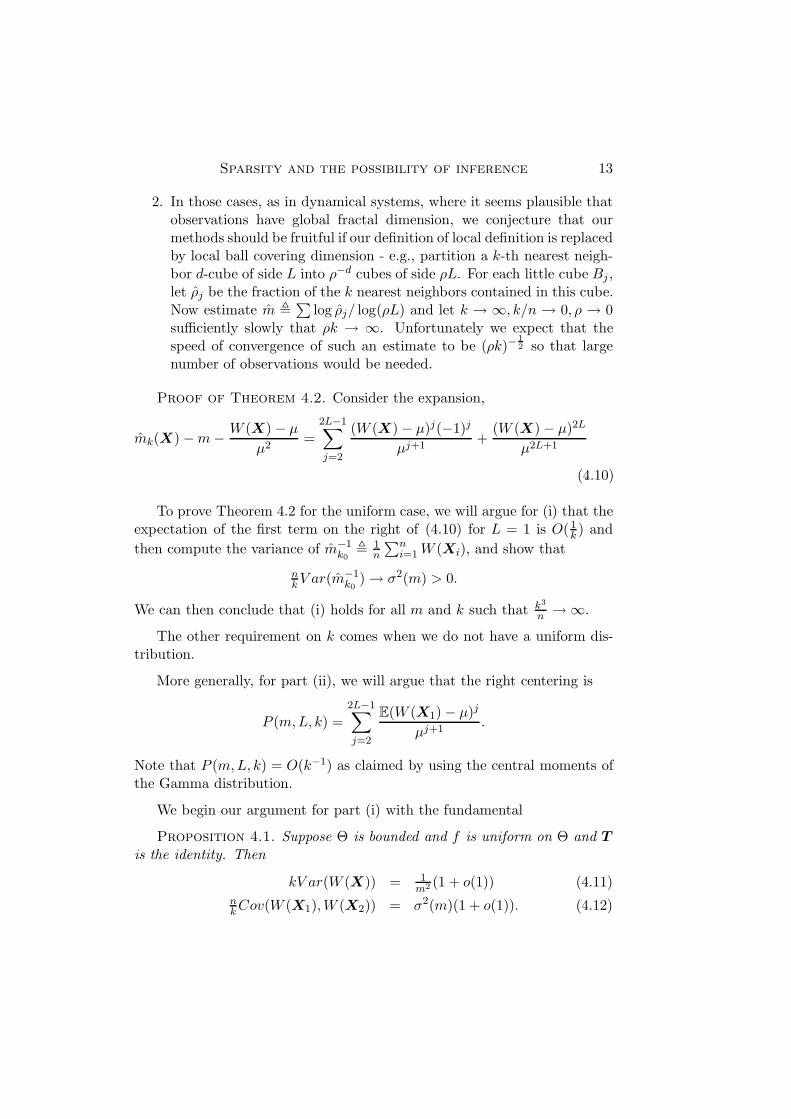
Proof of Theorem 4.2. Consider the expansion,
mk(X) ( m ( W (X) ( µ
µ2=
2L!1&
j=2
(W (X) ( µ)j((1)j
µj+1+
(W (X) ( µ)2L
µ2L+1
.(4.10)
To prove Theorem 4.2 for the uniform case, we will argue for (i) that theexpectation of the first term on the right of (4.10) for L = 1 is O( 1
k ) and
then compute the variance of m!1k0
! 1n
%ni=1 W (Xi), and show that
nk V ar(m!1
k0) $ "2(m) > 0.
We can then conclude that (i) holds for all m and k such that k3
n $ '.
The other requirement on k comes when we do not have a uniform dis-tribution.
More generally, for part (ii), we will argue that the right centering is
P (m,L, k) =2L!1&
j=2
E(W (X1) ( µ)j
µj+1.
Note that P (m,L, k) = O(k!1) as claimed by using the central moments ofthe Gamma distribution.
We begin our argument for part (i) with the fundamental
Proposition 4.1. Suppose % is bounded and f is uniform on % and T
is the identity. Then
kV ar(W (X)) = 1m2 (1 + o(1)) (4.11)
nk Cov(W (X1),W (X2)) = "2(m)(1 + o(1)). (4.12)
14 Peter J. Bickel and Donghui Yan
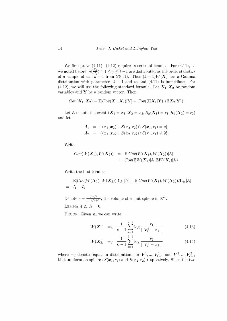
We first prove (4.11). (4.12) requires a series of lemmas. For (4.11), as
we noted before, n(Rj
Rk)m, 1 & j & k(1 are distributed as the order statistics
of a sample of size k ( 1 from U(0, 1). Thus (k ( 1)W (X) has a Gammadistribution with parameters k ( 1 and m and (4.11) is immediate. For(4.12), we will use the following standard formula. Let X1,X2 be randomvariables and Y be a random vector. Then
Cov(X1,X2) = E[Cov(X1,X2)|Y] + Cov((EX1|Y), (EX2|Y)).
Let A denote the event (X1 = x1,X2 = x2, Rk(X1) = r1, Rk(X2) = r2)and let
A1 = {(x1,x2) : S(x2, r2) 0 S(x1, r1) = 2}A2 = {(x1,x2) : S(x2, r2) 0 S(x1, r1) -= 2}.
Write
Cov(W (X1),W (X2)) = E[Cov(W (X1),W (X2))|A]
+ Cov(EW (X1)|A, EW (X2)|A).
Write the first term as
E[Cov(W (X1),W (X2)).1A1|A] + E[Cov(W (X1),W (X2)).1A2
|A]
= I1 + I2.
Denote c = $m/2
![m/2+1] , the volume of a unit sphere in Rm.
Lemma 4.2. I1 = 0.
Proof. Given A, we can write
W (X1) =d1
k ( 1
k!1&
i=1
logr1
3 V 1i ( x1 3
(4.13)
W (X2) =d1
k ( 1
k!1&
i=1
logr2
3 V 2i ( x2 3
(4.14)
where =d denotes equal in distribution, for V 11 , ...,V 1
k!1 and V 21 , ...,V 2
k!1i.i.d. uniform on spheres S(x1, r1) and S(x2, r2) respectively. Since the two
Sparsity and the possibility of inference 15
sequences of random variables V 11 , ...,V 1
k!1 and V 21 , ...,V 2
k!1 are conditionallyindependent on set A1,
Cov(W (X1),W (X2)).1A1|A
= E-)
W (X1) ( EW (X1)|A*)
W (X2) ( EW (X2)|A*
.1A1| A
.
= E
'/ 1
k ( 1
k!1&
i=1
logr1
3 V 1i ( x1 3
( µ0
.1A1|A
(
.
E
'/ 1
k ( 1
k!1&
i=1
logr2
3 V 2i ( x2 3
( µ0
.1A1|A
(
= 0.
Therefore I1 = E[Cov(W (X1),W (X2)).1A1|A)] = 0. !
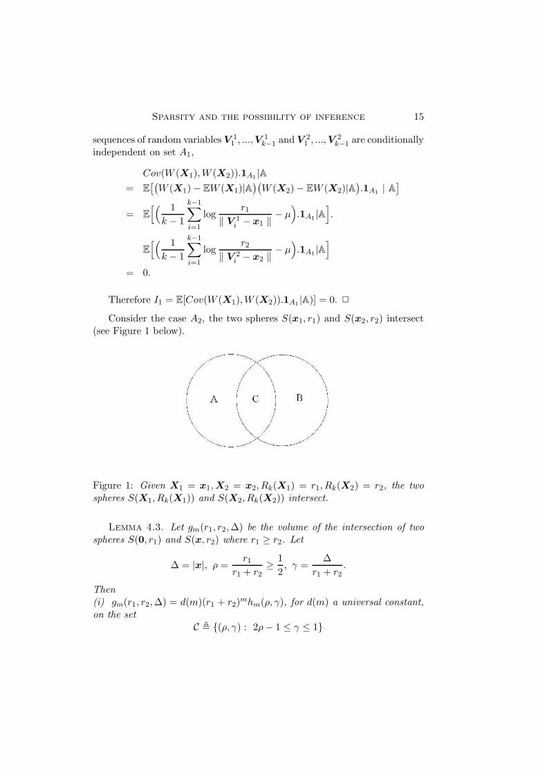
Consider the case A2, the two spheres S(x1, r1) and S(x2, r2) intersect(see Figure 1 below).
Figure 1: Given X1 = x1,X2 = x2, Rk(X1) = r1, Rk(X2) = r2, the twospheres S(X1, Rk(X1)) and S(X2, Rk(X2)) intersect.
Lemma 4.3. Let gm(r1, r2, &) be the volume of the intersection of twospheres S(0, r1) and S(x, r2) where r1 1 r2. Let
& = |x|, ( =r1
r1 + r21 1
2, ' =
&
r1 + r2.
Then(i) gm(r1, r2, &) = d(m)(r1 + r2)mhm((, '), for d(m) a universal constant,on the set
C ! {((, ') : 2(( 1 & ' & 1}
16 Peter J. Bickel and Donghui Yan
and(ii)
1
hm = 0, for ' 1 1hm = (1 ( ()mcm, for ' & 2(( 1
since ' > 1 is equivalent to & 1 r1 + r2 which means that the spheres aretangent or disjoint, while ' & 2( ( 1 is equivalent to & + r2 & r1 whichmeans that the smaller sphere is contained in the larger.
Proof. By definition
gm(r1, r2, &) =
+
...
+
S(0,r1)%S(x,r2)dx.
Without loss of generality assume x = (&, 0, ..., 0) and change to polarcoordinate (r,)1, ...,)m!1)
2
3
3
3
3
4
3
3
3
3
5
x1 = r sin)1... sin)m!2 cos)m!1
x2 = r sin)1... sin)m!2 sin)m!1
· · · · · ·xm!1 = r sin)1 cos)2
xm = r cos)1
where (r,)1, ...,)m!1) ! [0,') 4 [0,*) 4 [0,*) 4 [0, 2*). Then
gm(r1, r2, &) =
+
Trm!1
m!26
i=1
(sin)i)m!i!1drd$
where
T =
7
r2 & r21, r2 ( 2&r
m!26
i=1
(sin)i)m!i!1 + &2 & r2
2
8
.
Change variables to
v =r
r1 + r2.
Then
gm(r1, r2, &) = (r1 + r2)m
+
Uvm!1
m!26
i=1
(sin)i)m!i!1dvd$
where
U =
7
v2 & (2, v2 ( 2'vm!26
i=1
(sin)i)m!i!1 + '2 & (1 ( ()2
8
.
Sparsity and the possibility of inference 17
The result follows. !
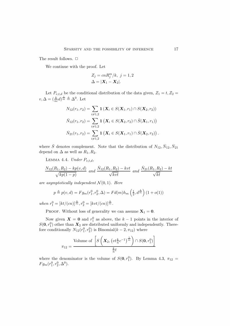
We continue with the proof. Let
Zj = cnRmj /k, j = 1, 2
& = |X1 ( X2|.
Let Pv,t,d be the conditional distribution of the data given, Z1 = t, Z2 =
v, & = ( kncd)
1m ! &0. Let
N12(r1, r2) =&
i&=1,2
1 (Xi ! S(X1, r1) 0 S(X2, r2))
N12(r1, r2) =&
i&=1,2
1)
Xi ! S(X2, r2) 0 S(X1, r1)*
N21(r1, r2) =&
i&=1,2
1)
Xi ! S(X1, r1) 0 S(X2, r2)*
.
where S denotes complement. Note that the distribution of N12, N12, N21
depend on & as well as R1, R2.
Lemma 4.4. Under Pv,t,d,
N12(R1, R2) ( kp(v, d)9
kp(1 ( p)and
N12(R1, R2) ( kvt.kvt
andN21(R1, R2) ( kt.
kt
are asymptotically independent N (0, 1). Here
p ! p(v, d) = Fgm(r01, r
02 , &) = Fd(m)hm
/
12 , d
1m
0
(1 + o(1))
when r01 = [kt/(cn)]
1m , r0
2 = [kvt/(cn)]1m .
Proof. Without loss of generality we can assume X1 = 0.
Now given X = 0 and r01 as above, the k ( 1 points in the interior of
S(0, r01) other than X2 are distributed uniformly and independently. There-
fore conditionally N12(r01, r
02) is Binomial(k ( 2,*12) where
*12 =
Volume of
:
S
;
X2,)
vt knc!1
*
1m
<
0 S(0, r01)
=
kn t
where the denominator is the volume of S(0, r01). By Lemma 4.3, *12 =
Fgm(r01, r
02, &0).
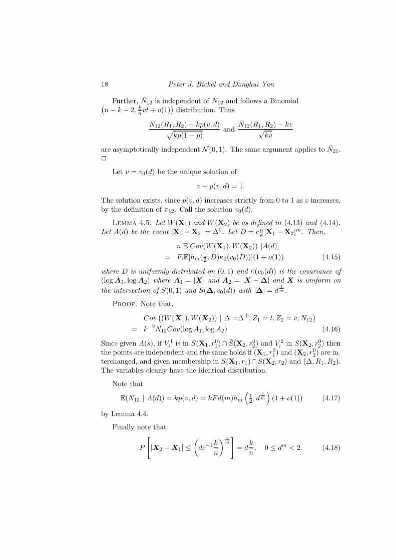
18 Peter J. Bickel and Donghui Yan
Further, N12 is independent of N12 and follows a Binomial)
n ( k ( 2, knvt + o(1)
*
distribution. Thus
N12(R1, R2) ( kp(v, d)9
kp(1 ( p)and
N12(R1, R2) ( kv.kv
are asymptotically independent N (0, 1). The same argument applies to N21.!
Let v = v0(d) be the unique solution of
v + p(v, d) = 1.
The solution exists, since p(v, d) increases strictly from 0 to 1 as v increases,by the definition of *12. Call the solution v0(d).
Lemma 4.5. Let W (X1) and W (X2) be as defined in (4.13) and (4.14).Let A(d) be the event |X1 (X2| = &0. Let D = cn
k |X1 ( X2|m. Then,
n.E[Cov(W (X1),W (X2)) |A(d)]
= F.E[hm(12 ,D)+0(v0(D))](1 + o(1)) (4.15)
where D is uniformly distributed on (0, 1) and +(v0(d)) is the covariance of(log A1, log A2) where A1 = |X| and A2 = |X (!| and X is uniform on
the intersection of S(0, 1) and S(!, v0(d)) with |!| = d1m .
Proof. Note that,
Cov)
(W (X1),W (X2)) | & =& 0, Z1 = t, Z2 = v,N12*
= k!2N12Cov(log A1, log A2) (4.16)
Since given A(s), if V 1i is in S(X1, r0
1)0 S(X2, r02) and V 2
i in S(X2, r02) then
the points are independent and the same holds if (X1, r01) and (X2, r0
2) are in-terchanged, and given membership in S(X1, r1)0S(X2, r2) and (&, R1, R2).The variables clearly have the identical distribution.
Note that
E(N12 | A(d)) = kp(v, d) = kFd(m)hm
/
12 , d
1m
0
(1 + o(1)) (4.17)
by Lemma 4.4.
Finally note that
P
>
|X2 ( X1| &;
dc!1 k
n
<1m
?
= dk
n, 0 & dm < 2. (4.18)
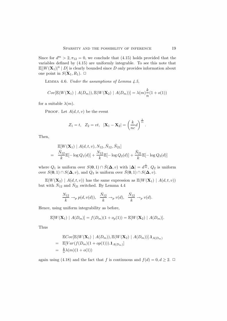
Sparsity and the possibility of inference 19
Since for dm > 2,*12 = 0, we conclude that (4.15) holds provided that thevariables defined by (4.15) are uniformly integrable. To see this note thatE[|W (X1)|4 | D] is clearly bounded since D only provides information aboutone point in S(X1, R1). !
Lemma 4.6. Under the assumptions of Lemma 4.5,
Cov[E(W (X1) | A(Dm)), E(W (X2) | A(Dm))] = $(m)k
n(1 + o(1))
for a suitable $(m).
Proof. Let A(d, t, v) be the event
Z1 = t, Z2 = vt, |X1 ( X2| =
;
k
ncd
<1m
.
Then,
E[W (X1) | A(d, t, v),N12, N12, N21]
=N12
kE[( log Q1(d)] +
N12
kE[( log Q2(d)] +
N21
kE[( log Q3(d)]
where Q1 is uniform over S(0, 1) 0 S(!, v) with |!| = d1m , Q2 is uniform
over S(0, 1) 0 S(!, v), and Q3 is uniform over S(0, 1) 0 S(!, v).
E(W (X2) | A(d, t, v)) has the same expression as E(W (X1) | A(d, t, v))but with N12 and N21 switched. By Lemma 4.4
N12
k$p p(d, v(d)),
N12
k$p v(d),
N12
k$p v(d).
Hence, using uniform integrability as before,
E[W (X1) | A(Dm)] = f(Dm)(1 + op(1)) = E[W (X2) | A(Dm)].
Thus
ECov[E(W (X1) | A(Dm)), E(W (X2) | A(Dm))].1A(Dm)
= E[V ar(f(Dm)(1 + op(1))).1A(Dm)]
= kn$(m)(1 + o(1))
again using (4.18) and the fact that f is continuous and f(d) = 0, d 1 2. !
20 Peter J. Bickel and Donghui Yan
A similar calculation applies to the variances of the individual terms in(4.10). This completes the proof of (ii) for the case T is identity on thefirst m coordinate vectors. To show that the results remain valid if T is asspecified and k(1+ m
4)/n $ 0, we simply apply the bounds of (4.5), (4.6) to
the joint density of (X1,X2,X) when computing covariances. For instance,
if B(s) ="
|T (U1) ( T (U2)| & (c!1s kn)
1m
#
P'
|T (U) ( T (U1)| & (c!1 kn)
1m , |T (U) ( T (U2)| & (c!1v0(s)
kn)
1m
!
! B(s)
= *(s, v0(s))/
1 + O-
( kn)
2m
.
0
since we can replace |T (U)(T (Uj)| by |(T (U)(x0)( (T (Uj)(x0)|. Thetheorem follows. !
Finally we sketch the proof of Theorem 4.3.
Proof of Theorem 3. We note that
mk(Xi) = h(Xi : Nk(Xi))
where Nk(Xi) is the set of neighbors up to the k-th of Xi. Therefore we canapply Theorem 3.4 of Chatterjee (2006) to establish Theorem 4.3 providedwe can show that
E(mk) = m
;
k ( 1
k ( 2
<
and (4.19)
V ar(mk) $ "2(m). (4.20)
Since'
1(k!1)mmk(Xi)
(!1has a Gamma(k ( 1, 1) distribution, (4.19) is im-
mediate.
We can similarly compute
V ar(mk(Xi)) = m2' (k ( 1)2
(k ( 2)(k ( 3)( (k ( 1)2
(k ( 2)2
(
= m2 (k ( 1)2
(k ( 2)21
k ( 3.
We are left to check that,
nCov(mk(X1), mk(X2)) " '(m,k)
Sparsity and the possibility of inference 21
for suitable '. Decomposing as before it is clear we need only be concernedwith
E-
U(X1)U(X2)!
!A(s).
and E-
U(X1)!
!A(s).
(4.21)
Given A2 and A(s), X2 = X1+(sc
kn)
1m V where V has a uniform distribution
on S(0, 2). By Lemma 4.3, *(s, v(s)) = Fhm(v, s). If we now define
W = Z
;
s
c
k
n
<! 1m
for Z uniform on S(0, r1)0S(1, r2), then W has a distribution which dependson s only.
Using this rescaling, the quantities in (4.21) depend only on the distri-bution of V and Nk(r2). Therefore for k bounded, the quantities in (4.21)depend on s and not on n to first order. But
P-
5 {A(t) : t & s}.
=s
2
k
n
for 0 & s & 2. From
nV ar(mk) = V ar(mk(X1)) + 2(n ( 1)Cov-
mk(X1), mk(X2).
,
the theorem follows in the uniform case. The general case is argued as in The-orem 4.2 again taking advantage of the boundedness of k. !
References
Abramovich, F., Benjamini, Y., Donoho, D.L., Johnstone, I.M.(2000). Adaptingto unknown sparsity by controlling the false discovery rate. Ann. Statist., 34,584-653.
Atkinson, A.C. (1980). A note on the generalized information criterion for choice of amodel. Biometrika, 67, 413-418.
Bickel, P.J. and Levina, E. (2004). Some theory of Fisher’s linear discriminant func-tion, ‘naive Bayes’, and some alternatives when there are many more variables thanobservations. Bernoulli, 10, 989-1010.
Bickel, P.J. and Levina, E. (2008)(i). Covariance Regularization by Thresholding.Ann. Statist. To appear.
Bickel, P.J. and Levina, E. (2008)(ii). Regularized Estimation of Large CovarianceMatrices. Ann. Statist., 36, 199-227.
Bickel, P.J. and Li, B. (2006). Regularization in Statistics. Test, 15, 271-344.
Bickel, P.J. and Li, B. (2007). Local polynomial regression on unknown manifolds.IMS Lecture Notes, 54.
22 Peter J. Bickel and Donghui Yan
Box, G.E.P. (1979). Robustness in the strategy of scientific model building, in Robust-ness in Statistics, R.L. Launer and G.N. Wilkinson, Editors. Academic Press, NewYork.
Breiman, L. and Friedman, J. H. (1985). Estimating Optimal Transformations forMultiple Regression and Correlation (with discussion). J. Amer. Statist. Assoc.,80, 580-619.
Candes, E. J., Donoho, D.L. (2004). New tight frames of curvelets and optimalrepresentations of objects with piecewise C2 singularities. Comm. Pure Appl.Math., 57, 219-266.
Candes, E. and Tao, T. (2007). The Dantzig selector: Statistical estimation when p ismuch larger than n (with discussion). Ann. Statist., 35, 2313-2351.
Chatterjee, S. (2006). A new method of normal approximation. Ann. Probab. Toappear.
Chen, S.S., Donoho, D.L., Saunders, M.A. (1998). Atomic decomposition by basispursuit. SIAM J. Sci. Comput., 20, 33-61.
D’aspremont, A., El Ghaoui, L., Jordan, M.I., Lanckriet, G.R.G. (2007). Adirect formulation for sparse PCA using semidefinite programming. SIAM Rev..49, 434-448.
Donoho, D.L., Elad, M. (2003). Optimally sparse representation in general (nonorthog-onal) dictionaries via l1 minimization. Proc. Natl. Acad. Sci., USA, 100, 2197-2202.
Donoho, D.L., Johnstone, I.M. (1994). Ideal denoising in an orthonormal basis chosenfrom a library of bases. C. R. Acad. Sci. Paris Sr. I Math., 319, 1317-1322.
Donoho, D.L., Johnstone, I.M. (1994). Minimax risk over lp-balls for lq-error. Probab.Theory Related Fields, 99, 277-303.
Donoho, D.L., Johnstone, I.M., Picard, D. and Kerkyacharian, G. (1995).Wavelet shrinkage: asymptotia? (with discussion). Journal of Royal StatisticalSociety (B), 301-369.
El Karoui, N. (2007). Spectrum estimation for large dimensional covariance matricesusing random matrix theory. Ann. Statist. To appear.
El Karoui, N. (2008). Operator norm consistent estimation of large dimensional sparsecovariance matrices. Ann. Statist. To appear.
Falconer, K. (1990). Fractal Geometry, Mathematical Foundations and Applications.Wiley.
Fan, J. and Lv, J. (2008). Sure independence screening for ultra-high dimensionalfeature space (with discussion). J. Roy Statist. Soc. (B). To appear.
Hastie, T., Tibshirani, R and Friedman, J. (2001). The Elements of StatisticalLearning: Data Mining, Inference, and Prediction. Springer, New York.
Johnstone, I.M. and Lu, A.Y. (2008). Sparse principal components analysis. J. Amer.Statist. Assoc. To appear.
Levina, E. and Bickel, P.J. (2005). Maximum likelihood estimation of the intrinsicdimension. Advances in NIPS 17.
Niyogi, P. (2007). Manifold Regularization and Semi-supervised Learning: Some Theo-retical Analyses. Technical Report, Computer Science Dept., University of Chicago.
Stone, C.J. (1977). Consistent nonparametric regression (with discussion). Ann. Statist.,5, 595-645.
Sparsity and the possibility of inference 23
Yang, Y. (2005). Can the strengths of AIC and BIC be shared? Biometrika, 92, 937-950.
Yukich, J. (2008). Point process stabilization methods and dimension estimation. Dis-crete Mathematics and Theoretical Computer Science, Nancy, France.
Peter J. Bickel
Department of Statistics
University of California, Berkeley
CA 94720, USA
E-mail: [email protected]
Donghui Yan
Department of Statistics
University of California, Berkeley
CA 94720, USA
E-mail: [email protected]
Paper received December 2008; revised .
![the law of large numbers & the CLT€¦ · strong law of large numbers i.i.d. (independent, identically distributed) random vars X 1, X 2, X 3, … X i has μ = E[X i] < ∞ Strong](https://static.fdocument.org/doc/165x107/5f89d20554e5db51a8543e6c/the-law-of-large-numbers-the-clt-strong-law-of-large-numbers-iid-independent.jpg)